| Issue |
A&A
Volume 647, March 2021
|
|
|---|---|---|
| Article Number | A73 | |
| Number of page(s) | 15 | |
| Section | Galactic structure, stellar clusters and populations | |
| DOI | https://doi.org/10.1051/0004-6361/202039864 | |
| Published online | 10 March 2021 | |
APOGEE DR16: A multi-zone chemical evolution model for the Galactic disc based on MCMC methods
1
Stellar Astrophysics Centre, Department of Physics and Astronomy, Aarhus University, Ny Munkegade 120, 8000 Aarhus C, Denmark
e-mail: spitoni@phys.au.dk
2
Center for Cosmology and AstroParticle Physics, The Ohio State University, 191 West Woodruff Avenue, Columbus, OH 43210, USA
3
Department of Astronomy, The Ohio State University, 140 West 18th Avenue, Columbus, OH 43210, USA
4
Dipartimento di Fisica, Sezione di Astronomia, Università di Trieste, Via G.B. Tiepolo 11, 34131 Trieste, Italy
5
INAF – Osservatorio Astronomico di Trieste, Via G.B. Tiepolo 11, 34131 Trieste, Italy
6
INFN – Sezione di Trieste, Via Valerio 2, 34100 Trieste, Italy
7
Technology University Dublin, School of Physics and Clinical & Optometric Sciences, Kevin Street, Saint Peter’s, Dublin 2 D08 X622, Ireland
8
SISSA – International School for Advanced Studies, Via Bonomea 265, 34136 Trieste, Italy
9
INAF – Osservatorio di Astrofisica e Scienza dello Spazio di Bologna, via Gobetti 93/3, 40129 Bologna, Italy
Received:
6
November
2020
Accepted:
21
January
2021
Context. The analysis of the latest release of the Apache Point Observatory Galactic Evolution Experiment project (APOGEE DR16) data suggests the existence of a clear distinction between two sequences of disc stars at different Galactocentric distances in the [α/Fe] versus [Fe/H] abundance ratio space: the so-called high-α sequence, classically associated with an old population of stars in the thick disc with high average [α/Fe], and the low-α sequence, which mostly comprises relatively young stars in the thin disc with low average [α/Fe].
Aims. We aim to constrain a multi-zone two-infall chemical evolution model designed for regions at different Galactocentric distances using measured chemical abundances from the APOGEE DR16 sample.
Methods. We performed a Bayesian analysis based on a Markov chain Monte Carlo method to fit our multi-zone two-infall chemical evolution model to the APOGEE DR16 data.
Results. An inside-out formation of the Galaxy disc naturally emerges from the best fit of our two-infall chemical-evolution model to APOGEE-DR16: Inner Galactic regions are assembled on shorter timescales compared to the external ones. In the outer disc (with radii R > 6 kpc), the chemical dilution due to a late accretion event of gas with a primordial chemical composition is the main driver of the [Mg/Fe] versus [Fe/H] abundance pattern in the low-α sequence. In the inner disc, in the framework of the two-infall model, we confirm the presence of an enriched gas infall in the low-α phase as suggested by chemo-dynamical models. Our Bayesian analysis of the recent APOGEE DR16 data suggests a significant delay time, ranging from ∼3.0 to 4.7 Gyr, between the first and second gas infall events for all the analysed Galactocentric regions. The best fit model reproduces several observational constraints such as: (i) the present-day stellar and gas surface density profiles; (ii) the present-day abundance gradients; (iii) the star formation rate profile; and (iv) the solar abundance values.
Conclusions. Our results propose a clear interpretation of the [Mg/Fe] versus [Fe/H] relations along the Galactic discs. The signatures of a delayed gas-rich merger which gives rise to a hiatus in the star formation history of the Galaxy are impressed in the [Mg/Fe] versus [Fe/H] relation, determining how the low-α stars are distributed in the abundance space at different Galactocentric distances, which is in agreement with the finding of recent chemo-dynamical simulations.
Key words: Galaxy: abundances / Galaxy: evolution / ISM: general / methods: statistical
© ESO 2021
1. Introduction
Our understanding of the formation and evolution of our Galaxy disc is essentially based on the study and interpretation of signatures imprinted in resolved stellar populations, such as their chemical and kinematic properties as traced by large surveys and observational campaigns. The current synergy between the Apache Point Observatory Galactic Evolution Experiment project (APOGEE; Majewski et al. 2017; in particular the latest data release DR16, Ahumada et al. 2020) and the Gaia mission (DR2; Gaia Collaboration 2018) offers an unparalleled opportunity to simultaneously rely on accurate spectroscopic and kinematic properties to constrain models of Galactic chemical evolution.
The analysis of the APOGEE DR16 data (Ahumada et al. 2020; Queiroz et al. 2020) suggests the existence of a clear distinction between two sequences of disc stars in the [α/Fe] versus [Fe/H] abundance ratio space: the so-called high-α and low-α sequences. This dichotomy in the chemical abundance ratio space has also been confirmed by the Gaia-ESO survey (e.g., Recio-Blanco et al. 2014; Rojas-Arriagada et al. 2016, 2017), the Archéologie avec Matisse Basée sur les aRchives de l’ESO project (AMBRE; Mikolaitis et al. 2017), and the Galactic Archaeology with HERMES survey (GALAH; Buder et al. 2019).
By analysing the APOKASC (APOGEE+ Kepler Asteroseismology Science Consortium) sample for the solar neighbourhood, Silva Aguirre et al. (2018) were able to pointed out that the two sequences are characterised by two different ages: the high-α stars have ages of ∼11 Gyr, while the low-α sequence peaks at ∼2 Gyr. Several theoretical models of the evolution of Galactic discs evolution have suggested that the bimodality may be strictly connected to a delayed gas accretion episode of primordial composition. By revising the classical two-infall chemical evolution model by Chiappini et al. (1997), Grisoni et al. (2017), and Spitoni et al. (2019a, 2020) have shown that a significant delay ranging from 4.5 to 5.5 Gyr between two consecutive episodes of gas accretion is needed to explain the dichotomy in the local APOKASC sample (Silva Aguirre et al. 2018). In particular, they predict that the star formation rate (SFR) has a minimum at an age of ∼8 Gyr. A similar quenching of star formation around the age of 8 Gyr was derived by Snaith et al. (2015) using the chemical abundances of Adibekyan et al. (2012) and the isochrone ages of Haywood et al. (2013) for solar-type stars. Moreover, Mor et al. (2019) found indications of a possible double-peaked star formation history with a minimum around 6 Gyr from the analysis of Gaia colour-magnitude diagrams. By analysing the High Accuracy Radial velocity Planet Searcher (HARPS) spectra of local solar twin stars, Nissen et al. (2020) found that the age-metallicity distribution has two distinct populations with a clear age dissection. The authors suggest that these two sequences may be interpreted as evidence of two episodes of accretion of gas onto the Galactic disc with quenching of star formation in between them, which is in agreement with the scenario proposed by Spitoni et al. (2019a, 2020).
In a cosmological framework, the existence of a double sequence was predicted for the first time by Calura & Menci (2009) who, by means of a semi-analytic model based on the extended Press and Schechter (Bond et al. 1991), modelled in post-processing the abundance pattern of a sample of model galaxies selected as Milky Way analogues. A second accretion phase after a prolonged period with a quenched star formation has been suggested by the dynamical models of Noguchi (2018) in which a first infall episode rapidly builds up the high-α sequence, but then the star formation is starved from the lack of gas supply from the intergalactic medium (IGM) until the shock-heated gas in the Galactic dark matter halo has radiatively cools down and is accreted by the Galaxy giving rise to a delayed second gas infall episode. In this framework, Noguchi (2018) found that the SFR of the Galactic disc is characterised by two distinct peaks separated by ∼5 Gyr. Moreover, the AURIGA simulations presented by Grand et al. (2018) clearly point out that a bimodal distribution in the [Fe/H]−[α/Fe] plane may be a consequence of a significantly lowered gas accretion rate at ages between 6 and 9 Gyr. In the framework of cosmological hydrodynamic simulations of Milky Way-like galaxies, Buck (2020) for example found that a dichotomy in the α-sequence is a generic consequence of a gas-rich merger occurred at a certain epoch in the evolution of the Galaxy, which destabilised the gaseous disc at high redshift.
The significant delay in the two-infall model of Spitoni et al. (2019a, 2020) has been discussed by Vincenzo et al. (2019) in the context of the stellar system accreted by the Galactic halo, AKA Gaia-Enceladus (Helmi et al. 2018; Koppelman et al. 2019). It was proposed that the mechanism that quenched the Milky Way star formation at high redshift was a major merger event with a satellite like Enceladus (by heating up the gas in the dark matter halo). This proposed scenario is in agreement with the recent Chaplin et al. (2020) study. They constrained the merging time with the observations of the very bright, naked-eye star ν Indi, finding at 68% confidence that the earliest the merger could have started was 11.6 Gyr ago.
As outlined by Hayden et al. (2015) and Queiroz et al. (2020), the two sequences in the [α/Fe] versus [Fe/H] abundance ratio relation from APOGEE have different features and trends throughout the Galactic disc. While the low-α sequence is distributed at increasingly lower metallicity towards the outer disc, it is found at super-solar values in the inner disc. Moreover, it is worth noticing that the ratio between the number of low-α and high-α stars increases when moving from the inner to the outer Galactic disc. Hence, the formation of the low-α sequence in the entire Galaxy seems to be more complex than a simple sequential process as assumed in the model of Spitoni et al. (2020) for the solar vicinity and may be driven by different physical processes. For instance, in the cosmological simulations presented by Agertz et al. (2020) and Renaud et al. (2020a,b), they concluded that the low-α sequence has been assembled through different physical process that interplay together in the whole disc. Two distinct channels of gas infall fuel the Galactic disc; a chemically enriched gas accretion event (by outflows from a massive galaxy with ∼1/3 of the Galactic mass at the time of the interaction) feeds the inner Galactic region, whereas a different one fuels the outer gas disc, which is inclined with respect to the main Galactic plane and has significantly poorer chemical content. However, their predicted low-α sequence is shifted towards larger [α/Fe] values than the APOGEE sample by ∼0.3 dex.
Recently, Palla et al. (2020) presented a revised Galactic chemical evolution model for the disc formation based on the two-infall scenario in order to reproduce the observed [Mg/Fe] versus [Fe/H] of APOGEE (Hayden et al. 2015) at different Galactocentric distances. Palla et al. (2020) proposed that a delay of tmax = 3.25 Gyr between the two gas infall events invoking an enriched gas infall to properly reproduce the inner disc [Mg/Fe] versus [Fe/H] abundance ratio. Khoperskov et al. (2021) found that in the infalling gas during inner thin disc formation phase is not primordial because the gaseous halo has been significantly polluted during the formation of the thick disc, providing a tight connection between chemical abundance patterns in the two Galactic disc components.
In this article, we present a multi-zone two-infall chemical evolution model with the aim to extend the results of Spitoni et al. (2019a, 2020) for the solar vicinity to the whole disc. We quantitatively infer the free parameters by fitting the APOGEE DR16 (Ahumada et al. 2020) abundance ratios at different Galactocentric distances using a Bayesian technique based on Markov chain Monte Carlo (MCMC) methods. The Bayesian analysis is now being widely used in testing the Galactic chemical evolution models (see e.g., Côté et al. 2017; Rybizki et al. 2017; Philcox et al. 2018; Frankel et al. 2018; Belfiore et al. 2019; Spitoni et al. 2020). In fact, thanks to the wealth of information from large surveys, large datasets are currently being exploited by means of statistic methods to constrain the parameters of Galactic chemical evolution models.
The paper is organised as follows. In Sect. 2, the observational data used in the Bayesian analysis are presented. In Sect. 3, we present the main characteristics of the multi-zone chemical evolution model adopted in this work, and describe the fitting method. In Sect. 4, we present our results, and finally in Sect. 5, we draw our conclusions.
2. The APOGEE DR16 sample
Here, following Spitoni et al. (2020), we use a Bayesian framework based on MCMC methods to fit a multi-zone Galactic chemical evolution model to the observed chemical abundances for Mg and Fe provided by APOGEE DR16 (Ahumada et al. 2020) and related Galactocentric distances and vertical heights above the Galactic plane, as found by the Gaia mission (DR2; Gaia Collaboration 2018).
Different methods have been introduced to compute proper Galactocentric distances. Luri et al. (2018) highlighted that the estimation of distances from parallaxes has to be addressed as a fully Bayesian inference problem, as shown in Bailer-Jones et al. 2018 for Gaia data. Moreover, in the Bayesian framework Queiroz et al. (2018) presented spectro-photometric distances estimated with the StarHorse tool which, in the case of APOGEE DR16, are derived from a set of photometric bands, APOGEE spectra and Gaia parallaxes. In this paper, we adopt the Galactocentric distances computed by Leung & Bovy (2019) and reported in the astroNN1 catalogue for APOGEE DR16 stars. To obtain precise distances for distant stars, Leung & Bovy (2019) designed a deep neural network, and trained it using precisely measured parallaxes of nearby stars in common between Gaia and APOGEE to determine the spectro-photometric distances for APOGEE stars. They included a flexible model to calibrate parallax zero-point biases in Gaia DR2 in order to avoid the propagation of systematic uncertainties present in the training data set to the inferred distances. On top of the versatility of the neural network, they employed a robust way of Bayesian deep learning that takes data uncertainties in the training set into account and also estimates uncertainties in predictions made with the neural network using the drop out variational inference. One major limitation of the method is the size of the training set it rests upon. Fortunately, the amount of data to train their algorithm will increase in the future thanks to new APOGEE and Gaia data releases and other spectroscopic surveys such as GALAH.
The Galactocentric positions and velocities used in the computation of the orbital properties are calculated assuming that the Galactocentric distance R⊙ from the Sun to the Galactic centre is 8.125 kpc (GRAVITY Collaboration 2018) and located 20.8 pc above the Galactic midplane (Bennett & Bovy 2019).
Stars that are part of the Galactic disc have been chosen with the same quality cuts suggested in Weinberg et al. (2019) assuming signal-to-noise ratio (S/N) > 80, logarithm of surface gravity between 1.0 < log g < 2.0 and vertical height |z|< 1 kpc to have cleaner trends in the [α/Fe] vs [Fe/H] abundance patterns at different radii for the MCMC fitting, since we adopt a one-zone chemical evolution model for each radial range of Galactocentric distances, which does not account for the small displacements observed in the APOGEE abundance distributions of the high-α and low-α sequences at high |z| (Hayden et al. 2015).
The uncertainties in metallicity reported in this compilation correspond to the internal precision, which are of the order of ∼0.01 dex. In the effort to better estimate systematic uncertainties, we added, as in Silva Aguirre et al. (2018), the median difference between APOGEE results for clusters and the standard literature values as reported in Table 3 of Tayar et al. (2017; ∼0.09 dex) in quadrature.
We have split the data into 3 concentric annular Galactic regions, each 4 kpc-wide, spanning the range between 2 and 14 kpc. In Fig. 1, it is clear that the further out stars (right panel, 10−14 kpc region) preferentially populate the low-α sequence in the [Mg/Fe] versus [Fe/H] relation, and few stars are located in the high-α population. Moreover, the more the regions are external, the more the locus of the low-α sequence is shifted towards lower metallicity. On the contrary, in the annular region enclosed between 2 and 6 kpc (left panel of Fig. 1), the low-α phase peaks at super-solar metallicity, however a clear bimodality is still evident as highlighted by the isodensity contours.
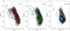 |
Fig. 1. Observed stellar [Mg/Fe] versus [Fe/H] abundance ratios from APOGEE DR16 (Ahumada et al. 2020) for three bins of different Galactocentric distances. The regions are 4 kpc-wide centred at 4 kpc (left panel), 8 kpc (middle panel) and 12 kpc (right panel), respectively. The contour lines enclose fractions of 0.90, 0.75, 0.60, 0.45, 0.30, 0.20, 0.05 of the total number of observed stars. Details on the data selection are reported in the text. |
We did not consider innermost regions with R < 2 kpc, because there the Galactic bulge is the dominant component and different Galactic chemical assumptions and prescriptions need to be applied (Matteucci et al. 2019, 2020; Griffith et al. 2020). The recent analysis of large samples from APOGEE DR16 data (Queiroz et al. 2020; Rojas-Arriagada et al. 2020) suggested that bulge structure could extend up to Galactocentric distances of 3−3.5 kpc. Hence, a partial contamination of bulge stars could in principle affect the region enclosed between 2 and 6 kpc. However, we checked that stars with Galactocentric distances selected in the range between 2 and 6 kpc give place to an almost identical distribution in the [Mg/Fe] versus [Fe/H] abundance ratio space as the ones enclosed in a region between 3 and 6 kpc.
The numbers of stars in the considered different annular regions are the following ones: 7440 in the zone centred at 4 kpc, 9169 in the one at 8 kpc, and 10 081 in the outermost region centred at 12 kpc. We believe that in these three zones the main trends of the Galactic disc in terms of the [Mg/Fe] versus [Fe/H] abundance as a function of the Galactocentric distance are imprinted. We have checked that the 4 kpc-wide region centred at 16 kpc has only 882 stars, almost all of which are in the low-α sequence.
3. Multi-zone chemical evolution model for the Galactic disc
In this section we present the main assumptions and characteristics of the multi-zone chemical evolution model which extends the previous ones introduced by Spitoni et al. (2019a, 2020) for the solar neighbourhood. After a brief explanation of the reasons for neglecting stellar migration effects, we describe the adopted MCMC methods.
3.1. Chemical evolution model prescriptions
We extend the chemical evolution model designed for the solar neighbourhood presented by Spitoni et al. (2019a, 2020) to different Galactocentric regions centred at 4 kpc, 8 kpc, and 12 kpc. Retaining the assumption that the Milky Way disc has been formed by two distinct accretion episodes of gas, we assume that the gas infall rate is a function of the Galactic distance R (Chiappini et al. 2001; Grisoni et al. 2018; Spitoni et al. 2009, 2019b) and is expressed by the following expression,
where τ1(R) and τ2(R) are the timescales of gas accretion for the formation of the high-α and low-α disc phase, respectively. The quantity θ in the Eq. (1) is the Heaviside step function. 𝒳1, i(R) and 𝒳2, i(R) are the abundance by mass of the element i in the infalling gas for the first and second gas infall, whereas tmax, R is the time of the maximum infall rate on the second accretion episode, that is to say it indicates the delay of the beginning of the second infall. Spitoni et al. (2019a) underlined the importance of a consistent delay of tmax ∼ 4 Gyr in the solar vicinity (defined as an annular region 2 kpc-wide centred at R = 8 kpc) in order to properly reproduce in the solar neighbourhood the stellar abundances and asteroseismic ages of the APOKASC data sample (Silva Aguirre et al. 2018). This finding was confirmed later by Spitoni et al. (2020) using a Bayesian analysis based on MCMC methods (see also Palla et al. 2020).
Finally, the coefficients 𝒩1(R) and 𝒩2(R) are obtained by imposing a fit to the observed current total surface mass density at different radii R with the following relations:
where σ1(R) and σ2(R) are the present-day total surface mass density of the high-α and low-α sequence stars, respectively, and tG is the age of the Galaxy.
Following Spitoni et al. (2020), we use the value of total surface density (sum of high-α and low-α) in the solar neighbourhood of 47.1 ± 3.4 M⊙ pc−2 as provided by McKee et al. (2015). In Spitoni et al. (2020) it was assumed that in the solar neighbourhood the total surface mass densities (σtot, ⊙ = σ1, ⊙ + σ2, ⊙) is constant, as given by McKee et al. (2015). The present-day total surface mass density at a certain Galactocentric distance R can be written as
after having imposed that the total mass declines with the radius through an exponential law and the scale-length of the disc is Rd = 3.5 kpc. In contrast with Palla et al. (2020) where different scale-lengths for the thick and thin disc phases were tested and assumed (see their Fig. 6), here we consider the ratio between the surface gas densities as a free parameter of the model.
Recalling that σ2/σ1 is the ratio between the low-α and high-α, the values of the present-day total surface mass densities σ2(R) and σ1(R) to insert in Eqs. (2) and (3) are the following ones:

The SFR is expressed as the Kennicutt (1998) law,
where σg is the gas surface density and k = 1.5 is the exponent. The quantity ν(t, R) is the star formation efficiency (SFE). Motivated by the theory of star formation induced by spiral density waves in Galactic discs (Wyse & Silk 1989), we consider a variable SFE as a function of the Galactocentric distance in the low-α phase. In several chemical evolution models (Colavitti et al. 2008; Spitoni et al. 2015; Grisoni et al. 2018; Palla et al. 2020) it has been claimed that observed abundance gradients in the Galactic disc may be explained by assuming higher SFE values in the inner regions than in the outer ones (along with the ‘inside-out’ formation scenario and radial gas flows).
Moreover, different infall episodes in principle could be characterised by different SFEs. In fact, in the classical two-infall model (Chiappini et al. 2001; Grisoni et al. 2017, 2019, 2020; Spitoni et al. 2020) the SFEs associated with the high-α and low-α sequences are different: ν1 = 2 Gyr−1 and ν2 = 1 Gyr−1 for the solar vicinity. We adopt the Scalo (1986) initial stellar mass function (IMF), constant in time and space.
Although an important ingredient of the Nidever et al. (2014) chemical evolution model to reproduce the APOGEE data was the inclusion of Galactic winds proportional to the SFR coupled to a variable loading factor, in this paper we do not consider outflows. In fact, while studying the Galactic fountains originated by the explosions of Type II SNe in OB associations, Melioli et al. (2008, 2009) and Spitoni et al. (2008, 2009) found that the ejected metals fall back close to the same Galactocentric region where they are delivered and thus do not modify significantly the chemical evolution of the disc as a whole.
As in Spitoni et al. (2019a, 2020), we adopt the same nucleosynthesis prescriptions as proposed by François et al. (2004) for Fe, Mg and Si. The authors artificially increased the Mg yields for massive stars from Woosley & Weaver (1995) to reproduce the solar Mg abundance. Mg yields from stars in the range 11−20 M⊙ have been increased by a factor of 7, whereas yields for stars with mass > 20 M⊙ are on average a factor ∼2 larger. No modifications are required for the yields of Fe, as computed for solar chemical composition. Concerning Si, only the yields of very massive stars (M > 40 M⊙) are increased by a factor of 2. Concerning Type Ia SNe, in order to preserve the observed [Mg/Fe] versus [Fe/H] pattern, the yields of Iwamoto et al. (1999) for Mg were increased by a factor of 5.
This set of yields has been widely used in the literature (Cescutti et al. 2007; Spitoni et al. 2014, 2015, 2017, 2019b; Mott et al. 2013; Vincenzo et al. 2019) and turned out to be able to reproduce the main features of the solar neighbourhood. We adopt the photospheric values of Asplund et al. (2005) as our solar reference abundances, in order to be consistent with the APOGEE DR16 release.
3.2. Stellar migration and Galactic chemical evolution
The existence of stellar radial migration is established beyond any doubts (see, e.g., Roškar et al. 2008; Schönrich & Binney 2009; Loebman et al. 2011; Minchev et al. 2012; Kubryk et al. 2013). The main physical mechanisms responsible for stellar migration are churning and blurring (e.g., Sellwood & Binney 2002; Minchev et al. 2011), as well as the overlap of the spiral and bar resonances on the disc (Minchev et al. 2011). However, the real impact of radial migration on the chemical evolution of the Galactic disc is still under debate.
Nidever et al. (2014) and Sharma et al. (2020) presented chemical evolution models where the dichotomy in the abundance space is entirely explainable only in terms of stellar migration. They concluded that the high-α disc has been built by migrator stars and gas of the thin disc.
In particular, the model presented by Sharma et al. (2020) assumed empirical tracks for the evolution of [α/Fe] and [Fe/H] as a function of time at different radii. These empirical age-metallicity relations may be inconsistent with their assumed empirical relations for the SFR as a function of time at different radii, which did not require a hiatus in the star formation between the high-α and low-α sequences, as predicted by the two-infall chemical evolution model and chemo-dynamical simulations. Finally, we note that stellar migration in Sharma et al. (2020) follows a parametric diffusion approach (e.g., Schönrich & Binney 2009).
On the contrary, the analysis of recent results from chemo-dynamical simulations has raised important doubts about the importance of stellar migration in the evolution of chemical abundance ratios, such as [α/Fe] versus [Fe/H], in the Galactic disc. For instance, by means of a self-consistent chemo-dynamical model for the Galactic disc evolution, Khoperskov et al. (2021) concluded that radial migration has a negligible effect on the [α/Fe] versus [Fe/H] distribution over time (the distribution is slightly smoothed by migrators from the inner and outer disc regions), suggesting the α-dichotomy is strictly linked to different star formation regimes over the Galaxy’s life.
Similar results are found by the cosmological simulation of Vincenzo & Kobayashi (2020). The authors concluded that the two main gas accretion episodes occurred 0−2 and 5−7 Gyr ago, determinant for the rise of the double sequence in the [α/Fe] versus [Fe/H] plot. In their Fig. 13, it is remarkable that the abundances in stars with ages smaller than 8 Gyr in the solar neighbourhood perfectly trace the gas phase abundances in the same region. They concluded that the signature impressed in the chemical abundances of the stars may be linked to infalling of primordial or poorly enriched gas. Supported by these results, we can safely assume that the stellar migration did not alter or affect much the [Mg/Fe] versus [Fe/H] evolution in our analysis which adopts Galactic annular regions 4 kpc-wide.
Although stellar migration has played an important role in Galactic evolution, i.e. in flattening of the radial metallicity profiles and affecting the [α/Fe]-age relation of thin-disc stars (Vincenzo & Kobayashi 2020), we investigate a complementary scenario with respect to that proposed by Sharma et al. (2020), in which the radial variation in the [α/Fe] versus [Fe/H] abundance have been entirely caused by the stellar migration.
3.3. Fitting the data with MCMC methods
As in Spitoni et al. (2020), we use a Bayesian analysis based on Markov chain Monte Carlo (MCMC) methods to find the best-fit chemical evolution models at different Galactocentric distances, R. Here, we briefly recall the main assumptions and refer the reader to Spitoni et al. (2020) for a more detailed description of the fitting method.
At a fixed R, the set of observables is xR = {[Mg/Fe], [Fe/H]} while the set of model parameters is ΘR = {τ1, τ2, tmax, σ2/σ1}. The adopted likelihood, ℒ, used to compute the posterior probability distribution can be written as
where N is the number of stars in a Galactic region corresponding to R. The quantities xn, j and σn, j are respectively the measured value of jth observable and its uncertainty for nth star. μn, j is the model value of the jth observable for the nth star. As underlined in Spitoni et al. (2020), the curve predicted by the two-infall model in the plane [Mg/Fe] versus [Fe/H] is multi-valued (see their Fig. 1). As a result, an observed data point in the [Fe/H]−[α/Fe] plane cannot be associated unambiguously to a point on the curve. To get through this problem they associated a data point to the closest value on the curve given a data point xn, j, defining the following ‘distance data-model’ function D,
where i runs over a set of discrete values on the curve. Hence, the closest point on the curve is μn, j = μn, j, i′ which fulfils the following relation:
Here, we present the priors on ΘR = {τ1, τ2, tmax, σ2/σ1}. We use uniform priors for all parameters, which are independent of the Galactocentric distances (i.e. priors are the same for all model runs at different R). In the classical two-infall model (Chiappini et al. 1997; Spitoni et al. 2020), the first gas infall is characterised by a short timescale of accretion in the solar neighbourhood, fixed at the value of τ1 = 1 Gyr. More recently, Grisoni et al. (2017, in order to reproduce the AMBRE thick disc), and Spitoni et al. (2019a) suggested a smaller value, τ1 = 0.1 Gyr. In the current study, we set a uniform prior on τ1 exploring the range 0 < τ1 < 7 Gyr. The second infall timescale, τ2, is connected to a slower accretion episode. We set a uniform prior on τ2 exploring the range 0 < τ2 < 14 Gyr. For the delay tmax we set a uniform prior exploring the range 0 < tmax < 14 Gyr.
Concerning the present-day ratio between the total surface mass densities σ2/σ1, we recall that Fuhrmann et al. (2017) derived in the solar vicinity a local mass density ratio between the thin and thick disc stars of 5.26, which becomes as low as 1.73 after correction for the difference in the scale height. While studying APOGEE stars, Mackereth et al. (2017) found that the relative contribution of low- to high-α is 5.5. In the solar annulus, Spitoni et al. (2020) found that the best models span the range between 3.2 and 4.3. In this work, studying different Galactic regions, we set this prior in the range, 0.1 < σ2/σ1 < 50.
The affine invariant MCMC ensemble sampler, “emcee: the mcmc hammer” code2, proposed by Goodman & Weare (2010), Foreman-Mackey et al. (2013) has been used to sample the posterior probability distribution.
4. Results
Here, we show predictions of chemical evolution models of the Galactic disc computed at different Galactocentric distances. In Sect. 4.1 we present and discuss our findings for chemical evolution models computed at 8 and 12 kpc, whereas the innermost region centred at 4 kpc is presented in Sect. 4.2. In Sect. 4.3 we interpret our results in terms of the “inside-out” formation scenario and we show a comparison between our predictions and some of the most important observables of the Galactic disc. In Sect. 4.4 the metallicity and the [Mg/Fe] distributions will be presented. Finally, in Sect. 4.5 we compare our findings with the chemical evolution predictions of the recent study presented by Palla et al. (2020).
4.1. Outer disc evolution: a tale of gas accretion and dilution
First, in this section we present the results of the best-fit chemical evolution model at 8 kpc, which was obtained by fitting the abundance ratios [Mg/Fe] and [Fe/H] of stars in the APOGEE DR16 sample using our Bayesian technique based on the MCMC methods. This model assumes infall episodes with primordial chemical composition for both high-α and low-α sequences (𝒳1 and 𝒳2 quantities in Eq. (1)) and different SFE: ν1 = 2 Gyr−1 and ν2 = 1 Gyr−1 (Chiappini et al. 1997; Grisoni et al. 2018; Spitoni et al. 2020; Palla et al. 2020). In Fig. 2 we show the posterior probability density function (PDF) of the chemical evolution model parameters, Θ⊙ = {τ1, τ2, tmax, σ2/σ1}, for our model at a Galactocentric distance of 8 kpc. We find a significant delay in the start of the second gas infall  Gyr, confirming the previous results of Spitoni et al. (2019a, 2020). The best model predicts a value of 5.635
 for the σ2/σ1 ratio, in accordance with the findings of Mackereth et al. (2017), Fuhrmann et al. (2017), Spitoni et al. (2020). Predicted infall timescales
  Gyr and
  Gyr are shorter than the ones of Spitoni et al. (2020). We recall that in that work the model was compared with the APOKASC sample by Silva Aguirre et al. (2018), which consisted of 1180 red giants in a narrower region in the solar vicinity (2 kpc-wide). The APOKASC sample has measured solar-like oscillations, allowing asteroseismic determination of stellar ages. In Spitoni et al. (2020), the determined stellar ages were used as additional constraint. Recall that here we adopt different selection criteria for stars following Weinberg et al. (2019) and Vincenzo & Kobayashi (2020).
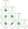 |
Fig. 2. Corner plot showing the posterior PDFs of the chemical evolution model parameters for the region at 8 kpc. For each parameter, the median and the 16th and 84th percentiles of the posterior PDF are shown with dashed lines above the marginalised PDF. The SFEs are fixed at values of 2 and 1 Gyr−1 for the high- and low-α phases, respectively. |
In fact, while the APOKASC sample shows absence of stars with [α/Fe] < −0.05 dex (see Fig. 1 in Spitoni et al. 2020), the sample adopted here has a significant fraction of low-α stars with [Mg/Fe] < −0.05 dex. Hence, the differences in the best-fit values for the infall timescales can be attributed to the differences in the data used in the two studies.
In Fig. 3 we compare the best-fit model computed at 8 kpc with the [Mg/Fe] versus [Fe/H] abundance ratios. The colour coding with the cumulative number of stars formed during the Galactic evolution shows that the bulk of the stars are formed during the low-α sequence. Moreover, the surface stellar mass density ΔM⋆ formed in different age bins as a function of age (see the inset plot of Fig. 3), clearly shows the existence of a low-α and high-α bimodality.
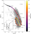 |
Fig. 3. Observed [Mg/Fe] versus [Fe/H] abundance ratios from APOGEE DR16 (Ahumada et al. 2020; grey points with associated errors) in the Galactocentric region between 6 and 10 kpc compared with the best-fit chemical evolution model (thick curve) in that region. As in Fig. 1, the contour lines enclose fractions of 0.90, 0.75, 0.60, 0.45, 0.30, 0.20, 0.05 of the total number of observed stars. The colour coding represents the cumulative number of stars formed during the Galactic evolution normalised to the total number Ntot. The open circles mark the model abundance ratios of stellar populations with different ages. In the inset we show the surface stellar mass density ΔM⋆ formed in different age bins as a function of age, where the bin sizes are delimited by the vertical dashed lines and correspond to the same age values as indicated in the [Mg/Fe] vs [Fe/H] plot. |
For the sake of clarity, in response to a question posed in Lian et al. (2020) we underline that this bimodality was already present in the best fit model of Spitoni et al. (2019a) who did not show the variation of the stellar mass content along with the chemical evolution tracks in their figures.
As illustrated in Spitoni et al. (2020, 2019a), the gas dilution originated by a strong second gas infall is a key process to explain APOKASC abundance ratios with our model. In particular, the second accretion event of pristine gas decreases the metallicity of the stellar populations born immediately after keeping a roughly constant [Mg/Fe] ratio since the accretion involves H and He but basically no metals. When star formation resumes, Type II SNe produce a steep bump in [Mg/Fe], which subsequently decreases at higher metallicities due to iron from Type Ia SNe (Matteucci et al. 2009; Bonaparte et al. 2013). This sequence produces a loop feature in the chemical evolution track of [Mg/Fe] versus [Fe/H]. We notice from the inset plot of Fig. 3 that a negligible mass fraction of low-α stars is formed during the dilution phase of the loop, with ages in the range between 9.7 and 9.2 Gyr (ΔM⋆ = 0.42 M⊙ pc−2, corresponding to ∼1.49% of the stellar mass formed during the second infall episode). In the ascending part of the loop with ages between 9.2 and 8.7 Gyr, the formed stellar mass is ΔM⋆ = 1.46 M⊙ pc−2 (∼5.18% of the predicted low-α sequence stellar mass). Finally, almost the totality of stellar mass is produced in the age interval between 8.7 Gyr and 0.2 Gyr, namely ΔM⋆ = 26.31 M⊙ pc−2, corresponding to ∼93.3% of the entire stellar mass produced during the second gas infall.
The ascendant part of the loop seems to pass through a region without many stars. We underline that the availability of additional observables in the MCMC analysis, as for instance precise asteroseismic ages, can potentially alleviate this apparent tension, leading to a smaller loop in the [α/Fe] versus [Fe/H] space, as shown in Spitoni et al. (2020).
We stress that, as shown in Spitoni et al. (2019a), it is likely that the loop feature is hidden inside the observational errors. Using a “synthetic” model (at each Galactic time a random error was assigned to the ages and metallicities of the stellar populations), Spitoni et al. (2019a) were capable to reproducing the data spread in the low-α sequence of the APOKASC sample (Silva Aguirre et al. 2018) in the [α/Fe] versus [Fe/H] abundance ratio space.
In Table 1, we compare the solar abundances of Fe, Mg, and Si predicted by our best fit model in the solar neighbourhood with Asplund et al. (2005) photospheric values. In the model, solar abundances are determined from the composition of the ISM at the time of the formation of the Sun (after 9.5 Gyr from the Big Bang). It is evident that our model is able to reproduce well the solar abundance ratios for these elements.
Observed solar chemical abundances compared with model predictions.
In Figs. 4 and 5 we show the results for the external region centred at 12 kpc. For this model we also assume primordial infall for both the high- and low-α sequences and different SFEs for the high- and low-α phases, ν1 = 2 Gyr−1 and ν1 = 0.5 Gyr−1, respectively. As we stated in Sect. 3.1, a lower SFE in outer Galactic regions has been assumed by several chemical evolution models (Colavitti et al. 2008; Spitoni et al. 2015; Grisoni et al. 2018; Palla et al. 2020) in order to reproduce abundance gradients (see Sect. 4.3).
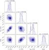 |
Fig. 4. Same as Fig. 2, but for the annular region enclosed between 10 and 14 kpc. The SFEs are fixed at values of 2 and 0.5 Gyr−1 for the high-α and low-α phases, respectively. |
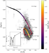 |
Fig. 5. Same as Fig. 3, but for the observed abundance [Mg/Fe] versus [Fe/H] ratio for stars with Galactocentric distances between 10 kpc and 14 kpc and the corresponding best-fit chemical evolution model. |
Comparing the best fit model parameters for the Galactic region centred at 8 kpc with those at 12 kpc, we note that longer timescales of gas accretion τ1(R) and τ2(R) are associated to more external region. Hence, the ‘inside-out’ formation scenario invoked by the classical two-infall model of Chiappini et al. (2001) in our model is a natural consequence of the fit to the APOGEE DR16 abundance ratio, as we shall discuss it thoroughly in Sect. 4.3.
4.2. Inner disc evolution: enriched gas infall and starbursts
Concerning the evolution of the inner disc, we consider the presence of an enriched gas infall for the low-α phase (𝒳2 quantity in Eq. (1)). In Palla et al. (2020), it was already pointed out that a primordial infall for the inner thin disc cannot explain the observed behaviour of the [α/Fe] versus [Fe/H] in the APOGEE data.
Different physical reasons may be associated with this enriched gas infall event. For instance, Palla et al. (2020) discussed that an enriched infall could partly be due to gas lost from the formation of the thick disc, Galactic halo or the Galactic bar which then gets mixed with a larger amount of infalling primordial gas as proposed by Gilmore & Wyse (1986). In Khoperskov et al. (2021), the infalling gas during inner thin disc formation phase is not primordial because the gaseous halo has been significantly polluted during the high-α disc formation, providing a tight connection between chemical abundance patterns in the high-α and low-α discs. Alternatively, as already mentioned in the Introduction, Renaud et al. (2020b) proposed that the Galaxy disc is fueled by two distinct gas flows and that the one responsible for the formation of the inner α sequence is enriched by outflows from massive galaxies (with ∼1/3 the Milky Way mass at the time of the interaction).
Following the best model prescriptions of Palla et al. (2020) for the inner thin disc, we impose that for the second gas infall (low-α), a chemical enrichment must be obtained from the model of the high-α disc phase corresponding to [Fe/H] = −0.5 dex. In Figs. 6 and 7 we present the chemical evolution model predictions for the region centred at 4 kpc assuming, for the high-α sequence, an SFE fixed at the value of ν1 = 3 Gyr−1. This higher value compared to external regions could be motivated by starburst episodes, as suggested by Agertz et al. (2020), Renaud et al. (2020a,b). The timescale τ2 of the second gas accretion episode and the ratio between low-α and high-α surface mass density σ2/σ1 are smaller compared to the external parts, in perfect agreement with the inside-out formation scenario (see Sect. 4.3 for a detailed discussion).
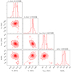 |
Fig. 6. Same as Fig. 2, but for the annular region enclosed between 2 and 6 kpc. For the second gas accretion episode, an enriched infall with [Fe/H] = −0.5 dex is considered. The SFEs are fixed at values of 3 and 1.5 Gyr−1 for the high-α and low-α phases, respectively. |
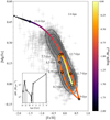 |
Fig. 7. Same as Fig. 3, but for stars of APOGEE DR16 (Ahumada et al. 2020) sample with Galactocentric distances between 2 and 6 kpc and the corresponding best fit chemical evolution model. Here, we considered a pre-enriched second gas infall with metallicity, [Fe/H] = −0.5 dex. The SFEs are fixed at values of 3 and 1.5 Gyr−1 for the high- and low-α phases, respectively. |
We also explore the possibility of an SFE fixed at the value of 2 Gyr−1 which as the same as in the outer regions. Although we found a similar [Mg/Fe] versus [Fe/H] relation, an extremely short (and maybe unrealistic) infall timescale of τ1 = 0.007 Gyr is required. We underline that such timescale is too small even compared to the Galactic bulge accretion timescale (Matteucci et al. 2019, 2020). Hence, a higher SFE (ν1 ∼ 3 Gyr−1) in the high-α disc phase provides more reasonable results in the two-infall framework.
4.3. Inside-out formation scenario and global properties of the Galactic disc
In Table 2 we summarise the best fit model parameters at different Galactocentric distances: the delay tmax, surface density ratio σ2/σ1, and infall timescales τ1 and τ2 values. The presence of a significant delay between the two infall episodes is a robust result, confirming the previous results of the works focusing on the solar neighbourhood (Spitoni et al. 2019a, 2020).
Main properties of our best-fit model at various Galactocentric distances.
In Fig. 8 we show that our model predictions are in favour of the ‘inside-out’ formation scenario: inner Galactic regions are assembled faster compared to the external one (Matteucci & Francois 1989; Chiappini et al. 2001; Schönrich & McMillan 2017; Frankel et al. 2019). In Fig. 1 data show that in the outer regions the locus of the low-α sequence shifts towards lower metallicity and in Fig. 8 we find that external Galactic regions are formed on longer accretion timescales τ2, hence the chemical enrichment is weaker and less efficient than the inner Galactic regions, leading to a lower metallicity. We recall that we imposed also a radial variation of the SFE.
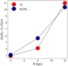 |
Fig. 8. Timescale τ2 for the gas accretion in the low-α phase and the ratio σ2/σ1 between the low-α and high-α total surface mass densities as a function of the Galactocentric distance are drawn with red and blue points, respectively. |
Moreover, in Fig. 1 the radial bin between 10 and 14 kpc has fewer high-α stars and we associate the more prominent low-α sequence to a larger surface density ratio σ2/σ1 compared to the innermost regions in agreement with Palla et al. (2020). An important result of this study is that extending the predictions for σ2/σ1 to the whole Galactic disc, we predict a clear and neat trend: the ratio increases with the Galactocentric distance (Fig. 8).
The Galactic ‘inside-out’ formation is well motivated by the dissipative collapse scenario (Larson 1976; Cole et al. 2000) and it has been a widely adopted assumption coupled with a variable SFE and the radial gas flows in order to reproduce the observed abundance gradients (Spitoni et al. 2015; Grisoni et al. 2018; Palla et al. 2020).
We have shown that the two-infall model of Spitoni et al. (2019a, 2020) can be extended to the whole disc admitting a more complex nature of the Galactic disc evolution instead of a simple sequential scenario, with the coexistence of different physical processes and different gas infall enrichment as a function of the Galactocentric distance. Moreover, with a quantitative estimation of the model free parameters using a Bayesian approach, we confirm the results of the chemical evolution model proposed by Palla et al. (2020), where an enriched gas infall has been invoked to reproduce the chemical evolution of the inner Galactic disc (see Sect. 4.5 for a detailed comparison with Palla et al. 2020 predictions). The proposed multi-zone chemical evolution model based on the MCMC methods to fit the abundance distributions of [Mg/Fe] versus [Fe/H] ratios from the APOGEE DR16 sample is also able to reproduce the other important observables of the Galactic disc.
In Fig. 9 we compare the observed abundance gradient for magnesium of Luck & Lambert (2011) and Genovali et al. (2015) with the one predicted by our best model computed at the present-day. To be consistent with these data sets, the model abundance ratios are referred to the solar value of Grevesse et al. (1996). It is clear that our model prediction well reproduces the observed abundance gradient.
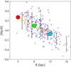 |
Fig. 9. Observed and predicted radial [Mg/H] present-day abundance gradient. The prediction of the best-fit models are indicated with big filled circles, connected with a yellow line. The observational data are the Cepheid observations from Luck & Lambert (2011; blue circles) and Genovali et al. (2015; blue diamonds with red edges). With the empty circles we report the average values and associated errors of the full data sample. |
It is clear from Fig. 10 that also the observed surface gas density profiles are well reproduced by our model. Concerning the present-day surface stellar mass density (see Fig. 11), the predicted value at 8 kpc is 34.2 M⊙ pc−2 in very good agreement with the observed local value of 33.4 ± 3 M⊙ (McKee et al. 2015). Assuming that the stellar surface density decreases exponentially outwards with a characteristic length-scale of R⋆ = 2.7 kpc (Kubryk et al. 2015), our model reproduces reasonably well this profile as shown in Fig. 11.
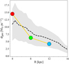 |
Fig. 10. Observed and predicted radial gas surface density gradient. The black dashed curve is the average between the Dame (1993) and Nakanishi & Sofue (2003, 2006) data sets. The grey shaded region represents the typical uncertainty at each radius, for which we adopt either 50% of the average (see Nakanishi & Sofue 2006) or half the difference between the minimum and maximum values in each radial bin (if larger). The big filled circles show the model predictions. |
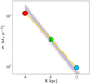 |
Fig. 11. Radial stellar surface stellar density profile of our model (big circles connected by a yellow line). The observed local stellar density is 33.4 ± 3 M⊙ pc−2 (McKee et al. 2015, small black dot and associated error bar). In our model we assume that the stellar profile decreases exponentially outwards with a characteristic scale-length of 2.7 kpc (Kubryk et al. 2015). The blue and grey shaded areas indicate zones within 1σ and 2σ, respectively. |
In the left panel of Fig. 12 we show that the predicted present-day SFR profile is in agreement with the observations by Rana (1991) and the following analytical fit of SN remnants compilation by Green (2014):
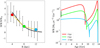 |
Fig. 12. Left panel: observed and predicted radial SFR density gradient relative to the solar neighbourhood. The model results are the big solid circles connected by a solid yellow line. The black line is the analytical form suggested by Green (2014) for the Milky Way SFR profile. The open circles with error bars are observational data from Rana (1991). Right panel: SFR evolution predicted by our best fit models computed at 4, 8, and 12 kpc. The dark green shaded area indicates the present-day measured range in the solar annulus by Prantzos et al. (2018). |
where R0 = 8 kpc, b = 2 and c = 5.1 (see Palla et al. 2020 for more details). In the temporal evolution of the predicted SFR at different Galactocentric distances reported in the right panel of Fig. 12, the two star formation phases (high-α and low-α stars) and the hiatus in between are evident. The delay tmax between the two infall gas episodes is longer as we move towards the inner region. Such a variation is statistically significant (see Table 2), and tmax values span the range between 3.0 and 4.7 Gyr. Longer cooling timescales due to a more intense star formation activity and stronger feedback are expected for the innermost Galactic regions at early times. Hence, we propose that in the inner (outer) regions the ISM gas needed more (less) time to cool down in order to begin the SF activity associated with the low-α sequence, leading to larger (smaller) values for tmax. This scenario is supported by several chemo-dynamical simulations in a cosmological framework where a hot gas phase is already in place at early times and the halo tends to inhibit gas filaments to penetrate into the central regions (Kereš et al. 2005; Dekel & Birnboim 2006; Brooks et al. 2009; Fernández et al. 2012; Grand et al. 2018).
In Fig. 13, we report the time evolution of the Type Ia SN and Type II SN rates. The present-day Type II SN rate in the whole Galactic disc predicted by our model is 0.93/[100 yr], a smaller value (but within 2σ error) than the observations of Li et al. (2011) which yield a value of 1.54 ± 0.32/[100 yr]. The predicted present-day Type Ia SN rate in the whole Galactic disc is 0.27/[100 yr], in good agreement with the value provided by Cappellaro & Turatto (1997) of 0.30 ± 0.20/[100 yr]. In the lower panel of Fig. 13 we also show the time evolution of the infall rate. We note that the present day value computed at 8 kpc is 1.01 M⊙ pc−2 Gyr−1, consistent with the range 0.3−1.5 M⊙ pc−2 Gyr−1 suggested by Matteucci (2012).
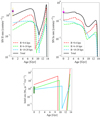 |
Fig. 13. Upper panels: observed and predicted Type II SN rates (left) and Type Ia SN rates (right) as a function of the Galactic age. The SN rates predicted for the whole disc are reported with the black solid lines, and they represent the sum of the contributions from different Galactic regions indicated with coloured dashed lines. The observed present-day Type II SN rate of Li et al. (2011, left panel) for the whole Galaxy is reported with the solid star (1σ and 2σ errors are indicated with grey and yellow bars, respectively) whereas the solid star in the right panel stands for Type Ia SN rate of Cappellaro & Turatto (1997) with the associated 1σ error bar. Lower panel: infall rate evolution predicted by our best fit models computed at 4 (red line), 8 (green line), and 12 kpc (light-blue line). The dark green shaded area indicates the present-day values in the solar annulus suggested by Matteucci (2012). |
In Fig. 14 the time evolution of the metallicity [M/H] and the [α/Fe] ratios computed at 4, 8, and 12 kpc are compared with the local APOKASC sample by Silva Aguirre et al. (2018). Here, α is computed by means of the sum of the abundances of Mg and Si. The metallicity [M/H] is computed, as in Silva Aguirre et al. (2018), using the following expression introduced by Salaris et al. (1993):
![$$ \begin{aligned} \mathrm{[M/H]} = \mathrm{[Fe/H]} + \log \left(0.638 \times 10^\mathrm{[\alpha /Fe]}+ 0.362 \right). \end{aligned} $$](/articles/aa/full_html/2021/03/aa39864-20/aa39864-20-eq28.gif)
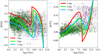 |
Fig. 14. Evolution of the [M/H] (left panel) and [α/Fe] (right panel) abundance ratios of our best-fit models computed at 4, 8, and 12 kpc compared with the abundances observed in a stellar sample in the solar annulus (Silva Aguirre et al. 2018). Magenta points depict the high-α population, whereas green points indicate the low-α one. As in Spitoni et al. (2019a, 2020), we have not taken into account young α-rich stars. |
We combine the abundance ratios [Fe/H] and [α/Fe] predicted by our model using this formulation to be consistent with the data. We notice that the best fit model at 8 kpc is very similar to the best model in Spitoni et al. (2019a) constrained by APOKASC abundance ratios and asteroseismic ages. Spitoni et al. (2019a) showed that the steep drop in [M/H] and bump in [α/Fe] associated with the second accretion episode (not obvious in the observations), are hidden behind the observational uncertainties.
The highest metallicity values are reached at any Galactic time by the innermost region. Different slopes in the [M/H] and [α/Fe] ratios characterize the evolution of the low-α sequences at different Galactcocentric distances. This is due to the interplay of different best-fit model values for timescale of accretion τ2, SFEs, and gas infall enrichment in diverse Galactic regions.
4.4. Metallicity and [Mg/Fe] distribution functions
In Fig. 15, it is shown that the predicted [Fe/H] distribution functions at different Galactocentric distances are generally in agreement with the data. To highlight once more the low-α and high-α bimodality, in Fig. 16 we show the [Mg/Fe] distributions, where we see that the APOGEE DR16 data in the annular region centred at 8 kpc exhibit two neat peaks. Although the best-fit model accounts for the observed bimodality and the median distribution value is consistent with the data, the predicted peaks are shifted towards higher [Mg/Fe] values. In the right panel of Fig. 16, we draw the same distribution but only for stars with [Fe/H] in the range between −0.2 and 0 dex (see the highlighted region in the enclosed plot). In this case, the predictions are in better agreement with the data.
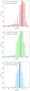 |
Fig. 15. Metallicity distributions predicted by the best-fit models (coloured histograms) computed at 4 kpc (upper panel), 8 kpc (middle panel), and 12 kpc (lower panel). The observed APOGEE DR16 distributions are shown by the black empty histograms. The vertical lines indicate the median values of each distribution. In each plot, the distributions are normalised to the corresponding maximum number of stars, Nmax. |
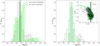 |
Fig. 16. Left panel: [Mg/Fe] distribution predicted by our best-fit model computed at 8 kpc (green histogram) compared with the APOGEE data in stars with Galactocentric distances between 6 and 10 kpc. Black and green vertical dashed lines indicate the median values of the data and model, respectively. Distributions are normalised to the corresponding maximum number of stars, Nmax. Right panel: same as the left panel, but computed for a limited metallicity range, −0.2 dex ≤ [Fe/H] ≤ 0 dex, as highlighted by the green shaded area in the inset. |
The reason why the full data set seems in contrast with model is largely due to the large uncertainty in the assumed stellar nucleosynthesis yields of Mg from massive stars, which cause the model to have higher [Mg/Fe] ratios (∼0.45 dex) at low [Fe/H] than the observations from APOGEE. Moreover, our assumption of a bottom-heavy IMF (Scalo 1986) slows down the time evolution of the [Fe/H] abundances in the ISM, creating a bias towards higher [Mg/Fe] ratios after each infall event. Additionally, since two-infall model is an approximate representation of the truth, significantly larger number of stars in the low-alpha sequence compared to the high-alpha can compromise the fit for the high-α sequence (as it gets less weight in the optimisation process presented in Sect. 3.3). A better agreement is achieved for the external region centred at 12 kpc as shown in Fig. 17, where the position of two peaks and the median value of the distribution are in good agreement with the data.
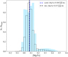 |
Fig. 17. [Mg/Fe] distribution predicted by our best-fit model computed at 12 kpc (blue histogram) compared with the APOGEE data in stars with Galactocentric distances between 10 and 14 kpc. Black and blue vertical lines indicate the median values of the data and model, respectively. |
In Fig. 18 the observed and predicted [Mg/Fe] distribution for the region centred at 4 kpc are compared. Once again, we see that the median value and the location of the two peaks are quite different from the data. In order to understand this discrepancy, we ran a new model with the same best-fit parameters as in Table 2 for the 4 kpc case, but with a smaller surface mass density σ2/σ1 ratio. In Fig. 19, we show the predicted [Mg/Fe] versus [Fe/H] relation and the [Mg/Fe] distribution function imposing σ2/σ1 = 1. In the upper panel of Fig. 19, we note that, as expected, the maximum [Mg/Fe] value reached in the low-α sequence is smaller compared to the one in Fig. 7 (with σ2/σ1 = 3.8) because of the smaller mass associated with the low-α phase as clearly shown in the inset plots of Figs. 7 and 19. In fact, the model with the lowest σ2/σ1 ratio presents the highest increase on stellar mass ΔM⋆ in the high-α phase.
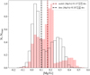 |
Fig. 18. [Mg/Fe] distribution predicted by our best-fit model computed at 4 kpc (red histogram) compared with the APOGEE data in a stellar sample with Galactocentric distances between 2 and 6 kpc. Black and red vertical lines indicate the median values of the data and model, respectively. |
In the lower panel of Fig. 19, we can appreciate that the model reproduces better the data than the results reported in Fig. 18 given also the intrinsic uncertainties due to the Mg stellar yields from massive stars and IMF. In fact, the median values of the predicted [Mg/Fe] and observed data are pretty similar. In conclusion, a smaller σ2/σ1 has a double effect: (i) the peak of the [Mg/Fe] abundance associated with the low-α is shifted towards smaller values, and (ii) an increase on the number of the high-α stars (the second peak in the distribution has a higher number of stars with larger [Mg/Fe] values than in Fig. 18).
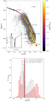 |
Fig. 19. APOGEE DR16 data in the region 2−6 kpc compared with model predictions computed at 4 kpc with the same best-fit parameters as in the first column of Table 2 but with the surface mass density ratio σ2/σ1 fixed at the value of 1. Upper panel: [Mg/Fe] versus [Fe/H] abundance ratios. As in Fig. 1, the contour lines enclose fractions of 0.90, 0.75, 0.60, 0.45, 0.30, 0.20, 0.05 of the total number of observed stars. The colour coding represents the cumulative number of stars formed during the Galactic evolution normalised to the total number Ntot. The open circles mark the model abundance ratios of stellar populations with different ages. In the inset we show the surface stellar mass density ΔM⋆ formed in different age bins as a function of age, where the bin sizes are delimited by the vertical dashed lines and correspond to the same age values as indicated in the [Mg/Fe] vs [Fe/H] plot. Lower panel: [Mg/Fe] distributions. Black and red vertical lines represent the median values of the data and model, respectively. |
4.5. Comparison with Palla et al. (2020)
Recently, Palla et al. (2020) presented a revised Galactic chemical evolution model for the disc formation based on the two-infall scenario. In agreement with our findings, their best model suggests that a variable SFE should be acting together with the ‘inside-out’ mechanism for the low-α disc formation. In addition, they claimed that radial gas inflows can help to create an abundance gradient confirming the findings of Spitoni et al. (2015) and Grisoni et al. (2018).
In order to reproduce the observed [Mg/Fe] versus [Fe/H] of APOGEE (Hayden et al. 2015) at different Galactocentric distances, Palla et al. (2020) proposed a delay of tmax = 3.25 Gyr between the two gas infall events, in agreement with the work presented here and Spitoni et al. (2019a, 2020). In particular, they invoked an enriched gas infall to properly reproduce the inner disc [Mg/Fe] versus [Fe/H] abundance ratio, in accordance with our study (see Sect. 4.2).
Differences in the chemical evolution tracks in the innermost disc region are primarily due to the different stellar nucleosynthesis prescriptions. Here, we adopt the yield collection proposed by François et al. (2004), whereas Palla et al. (2020) used those from Romano et al. (2010). Moreover, our results are based on a Bayesian analysis to fit the latest APOGEE DR16 data (Ahumada et al. 2020). Finally, Palla et al. (2020) impose a different length-scale for the two disc components instead of a variable ratio between the low-α and high-α surface mass densities. Notwithstanding all these differences, our model and the one of Palla et al. (2020) share a similar growth of the Galactic disc following the ‘inside-out’ scenario and predict pretty similar metallicity distribution functions.
5. Conclusions
We have presented a multi-zone chemical evolution model designed for the whole Galactic disc constrained by chemical abundance ratios of APOGEE DR16 (Ahumada et al. 2020) data using the Bayesian analysis presented in Spitoni et al. (2020). In this study, we have considered four free parameters: accretion timescales τ1 and τ2, delay tmax and present-day surface mass density ratio σ2/σ1.
Our main conclusions can be summarised as follows.
-
The Bayesian analysis based on the recent APOGEE DR16 data (Ahumada et al. 2020) suggests the presence of a significant delay time between the two gas infall episodes for the thick-disc and thin-disc formation in all analysed Galactocentric regions. We find that the best values for the delay times are in the range between 3 and 4.7 Gyr, confirming the findings of Spitoni et al. (2019a, 2020) for the solar neighbourhood based on the APOKASC data.
-
An inside-out formation of the thin-disc of our Galaxy naturally emerges from the best fit of our multi-zone chemical-evolution model to APOGEE-DR16 data: inner Galactic regions are assembled on shorter timescales than external Galactic zones. Moreover, our best-fit model predicts larger σ2/σ1 (ratio of low-α to high-α surface mass densities) values towards outer Galactic regions (see Fig. 8), in agreement with the fact that as we move towards external regions, the APOGEE DR16 data sample presents less and less stars in the high-α phase compared to the low-α sequence (Queiroz et al. 2020).
-
In outer disc regions with Galactocentric distances R > 6 kpc, the chemical dilution originating from a late gas accretion event with primordial chemical composition is the main driver of the [Mg/Fe] versus [Fe/H] abundance pattern in the low-α phase, extending the findings of the models presented by Spitoni et al. (2019a, 2020) for the solar neighbourhood.
-
In the inner disc, for the two-infall model to work, an enriched gas infall for the formation of low-α sequence stars is required to reproduce the observed data as suggested by Palla et al. (2020). Different physical explanations could be invoked: the gas might be enriched with metals from outflows originated in massive galaxies (Agertz et al. 2020; Renaud et al. 2020a,b), or it could be due to gas lost from the formation of the thick disc, which then gets mixed with a larger amount of infalling primordial gas (Gilmore & Wyse 1986).
-
Our model reproduces important observational constraints for the chemical evolution of the whole disc reasonably well, such as the present-day profiles of the SFR, the stellar and gas surface densities. Moreover, the predicted abundance gradient is in good agreement with the observations, thanks to the longer timescales of accretion in the outer regions and to a variable SFE for the low-α sequence. In the solar neighbourhood, the model is able to reproduce the solar photospheric abundance values of Asplund et al. (2005).
The above mentioned results suggest that the signatures of a delayed gas-rich merger giving rise to a hiatus in the star formation history are impressed in the [Mg/Fe] versus [Fe/H] relation and determine the distribution of the low-α stars in the abundance space at different Galactocentric distances.
Acknowledgments
Funding for the Stellar Astrophysics Centre is provided by The Danish National Research Foundation (Grant agreement no.: DNRF106). E. Spitoni and V. Silva Aguirre acknowledge support from the Independent Research Fund Denmark (Research grant 7027-00096B). F. Vincenzo acknowledges the support of a Fellowship from the Center for Cosmology and AstroParticle Physics at The Ohio State University. V. Grisoni acknowledges financial support at SISSA from the European Social Fund operational Programme 2014/2020 of the autonomous region Friuli Venezia Giulia. F. Calura acknowledges support from grant PRIN MIUR 2017 – 20173ML3WW 001 and from the INAF main-stream (1.05.01.86.31). In this work, we have made use of SDSS-IV APOGEE-2 DR16 data. Funding for the Sloan Digital Sky Survey IV has been provided by the Alfred P. Sloan Foundation, the US Department of Energy Office of Science, and the Participating Institutions. SDSS-IV acknowledges support and resources from the Center for High-Performance Computing at the University of Utah. The SDSS website is www.sdss.org. SDSS is managed by the Astrophysical Research Consortium for the Participating Institutions of the SDSS Collaboration which are listed at www.sdss.org/collaboration/affiliations/. This work has made use of data from the European Space Agency (ESA) mission Gaia (https://www.cosmos.esa.int/gaia), processed by the Gaia Data Processing and Analysis Consortium (DPAC, https://www.cosmos.esa.int/web/gaia/dpac/consortium). Funding for the DPAC has been provided by national institutions, in particular the institutions participating in the Gaia Multilateral Agreement.
References
- Adibekyan, V. Z., Sousa, S. G., Santos, N. C., et al. 2012, A&A, 545, A32 [NASA ADS] [CrossRef] [EDP Sciences] [Google Scholar]
- Agertz, O., Renaud, F., Feltzing, S., et al. 2020, MNRAS, submitted [arXiv:2006.06008] [Google Scholar]
- Ahumada, R., Allende Prieto, C., Almeida, A., et al. 2020, ApJS, 249, 3 [CrossRef] [Google Scholar]
- Asplund, M., Grevesse, N., & Sauval, A. J. 2005, in Cosmic Abundances as Records of Stellar Evolution and Nucleosynthesis, eds. T. G. Barnes, III, & F. N. Bash, ASP Conf. Ser., 336, 25 [Google Scholar]
- Bailer-Jones, C. A. L., Rybizki, J., Fouesneau, M., Mantelet, G., & Andrae, R. 2018, AJ, 156, 58 [NASA ADS] [CrossRef] [Google Scholar]
- Belfiore, F., Vincenzo, F., Maiolino, R., & Matteucci, F. 2019, MNRAS, 487, 456 [NASA ADS] [CrossRef] [Google Scholar]
- Bennett, M., & Bovy, J. 2019, MNRAS, 482, 1417 [NASA ADS] [CrossRef] [Google Scholar]
- Bonaparte, I., Matteucci, F., Recchi, S., et al. 2013, MNRAS, 435, 2460 [NASA ADS] [CrossRef] [Google Scholar]
- Bond, J. R., Cole, S., Efstathiou, G., & Kaiser, N. 1991, ApJ, 379, 440 [NASA ADS] [CrossRef] [Google Scholar]
- Brooks, A. M., Governato, F., Quinn, T., Brook, C. B., & Wadsley, J. 2009, ApJ, 694, 396 [NASA ADS] [CrossRef] [Google Scholar]
- Buck, T. 2020, MNRAS, 491, 5435 [NASA ADS] [CrossRef] [Google Scholar]
- Buder, S., Lind, K., Ness, M. K., et al. 2019, A&A, 624, A19 [NASA ADS] [CrossRef] [EDP Sciences] [Google Scholar]
- Calura, F., & Menci, N. 2009, MNRAS, 400, 1347 [NASA ADS] [CrossRef] [Google Scholar]
- Cappellaro, E., & Turatto, M. 1997, in NATO Advanced Science Institutes (ASI) Series C, eds. P. Ruiz-Lapuente, R. Canal, & J. Isern, 486, 77 [Google Scholar]
- Cescutti, G., Matteucci, F., François, P., & Chiappini, C. 2007, A&A, 462, 943 [NASA ADS] [CrossRef] [EDP Sciences] [Google Scholar]
- Chaplin, W. J., Serenelli, A. M., Miglio, A., et al. 2020, Nat. Astron., 4, 382 [Google Scholar]
- Chiappini, C., Matteucci, F., & Gratton, R. 1997, ApJ, 477, 765 [Google Scholar]
- Chiappini, C., Matteucci, F., & Romano, D. 2001, ApJ, 554, 1044 [Google Scholar]
- Colavitti, E., Matteucci, F., & Murante, G. 2008, A&A, 483, 401 [NASA ADS] [CrossRef] [EDP Sciences] [Google Scholar]
- Cole, S., Lacey, C. G., Baugh, C. M., & Frenk, C. S. 2000, MNRAS, 319, 168 [NASA ADS] [CrossRef] [Google Scholar]
- Côté, B., O’Shea, B. W., Ritter, C., Herwig, F., & Venn, K. A. 2017, ApJ, 835, 128 [NASA ADS] [CrossRef] [Google Scholar]
- Dame, T. M. 1993, in Back to the Galaxy, eds. S. S. Holt, & F. Verter, AIP Conf. Ser., 278, 267 [Google Scholar]
- Dekel, A., & Birnboim, Y. 2006, MNRAS, 368, 2 [NASA ADS] [CrossRef] [Google Scholar]
- Fernández, X., Joung, M. R., & Putman, M. E. 2012, ApJ, 749, 181 [NASA ADS] [CrossRef] [Google Scholar]
- Foreman-Mackey, D., Hogg, D. W., Lang, D., & Goodman, J. 2013, PASP, 125, 306 [Google Scholar]
- François, P., Matteucci, F., Cayrel, R., et al. 2004, A&A, 421, 613 [NASA ADS] [CrossRef] [EDP Sciences] [Google Scholar]
- Frankel, N., Rix, H.-W., Ting, Y.-S., Ness, M., & Hogg, D. W. 2018, ApJ, 865, 96 [Google Scholar]
- Frankel, N., Sanders, J., Rix, H.-W., Ting, Y.-S., & Ness, M. 2019, ApJ, 884, 99 [Google Scholar]
- Fuhrmann, K., Chini, R., Kaderhandt, L., & Chen, Z. 2017, MNRAS, 464, 2610 [Google Scholar]
- Gaia Collaboration (Katz, D., et al.) 2018, A&A, 616, A11 [NASA ADS] [CrossRef] [EDP Sciences] [Google Scholar]
- Genovali, K., Lemasle, B., da Silva, R., et al. 2015, A&A, 580, A17 [NASA ADS] [CrossRef] [EDP Sciences] [Google Scholar]
- Gilmore, G., & Wyse, R. F. G. 1986, Nature, 322, 806 [NASA ADS] [CrossRef] [Google Scholar]
- Goodman, J., & Weare, J. 2010, Commun. Appl. Math. Comput. Sci., 5, 65 [Google Scholar]
- Grand, R. J. J., Bustamante, S., Gómez, F. A., et al. 2018, MNRAS, 474, 3629 [NASA ADS] [CrossRef] [Google Scholar]
- GRAVITY Collaboration (Abuter, R., et al.) 2018, A&A, 615, L15 [NASA ADS] [CrossRef] [EDP Sciences] [Google Scholar]
- Green, D. A. 2014, in Supernova Environmental Impacts, eds. A. Ray, & R. A. McCray, IAU Symp., 296, 188 [NASA ADS] [Google Scholar]
- Grevesse, N., Noels, A., & Sauval, A. J. 1996, in Cosmic Abundances, eds. S. S. Holt, & G. Sonneborn, ASP Conf. Ser., 99, 117 [Google Scholar]
- Griffith, E., Weinberg, D. H., Johnson, J. A., et al. 2020, ArXiv e-prints [arXiv:2009.05063] [Google Scholar]
- Grisoni, V., Spitoni, E., Matteucci, F., et al. 2017, MNRAS, 472, 3637 [Google Scholar]
- Grisoni, V., Spitoni, E., & Matteucci, F. 2018, MNRAS, 481, 2570 [NASA ADS] [Google Scholar]
- Grisoni, V., Matteucci, F., Romano, D., & Fu, X. 2019, MNRAS, 489, 3539 [NASA ADS] [CrossRef] [Google Scholar]
- Grisoni, V., Romano, D., Spitoni, E., et al. 2020, MNRAS, 498, 1252 [CrossRef] [Google Scholar]
- Hayden, M. R., Bovy, J., Holtzman, J. A., et al. 2015, ApJ, 808, 132 [Google Scholar]
- Haywood, M., Di Matteo, P., Lehnert, M. D., Katz, D., & Gómez, A. 2013, A&A, 560, A109 [NASA ADS] [CrossRef] [EDP Sciences] [Google Scholar]
- Helmi, A., Babusiaux, C., Koppelman, H. H., et al. 2018, Nature, 563, 85 [NASA ADS] [CrossRef] [Google Scholar]
- Iwamoto, K., Brachwitz, F., Nomoto, K., et al. 1999, ApJS, 125, 439 [NASA ADS] [CrossRef] [MathSciNet] [Google Scholar]
- Kennicutt, R. C., Jr. 1998, ApJ, 498, 541 [NASA ADS] [CrossRef] [Google Scholar]
- Kereš, D., Katz, N., Weinberg, D. H., & Davé, R. 2005, MNRAS, 363, 2 [Google Scholar]
- Khoperskov, S., Haywood, M., Snaith, O., et al. 2021, MNRAS, 501, 5176 [NASA ADS] [CrossRef] [Google Scholar]
- Koppelman, H. H., Helmi, A., Massari, D., Price-Whelan, A. M., & Starkenburg, T. K. 2019, A&A, 631, L9 [NASA ADS] [CrossRef] [EDP Sciences] [Google Scholar]
- Kubryk, M., Prantzos, N., & Athanassoula, E. 2013, MNRAS, 436, 1479 [NASA ADS] [CrossRef] [Google Scholar]
- Kubryk, M., Prantzos, N., & Athanassoula, E. 2015, A&A, 580, A126 [NASA ADS] [CrossRef] [EDP Sciences] [Google Scholar]
- Larson, R. B. 1976, MNRAS, 176, 31 [NASA ADS] [CrossRef] [Google Scholar]
- Leung, H. W., & Bovy, J. 2019, MNRAS, 489, 2079 [NASA ADS] [CrossRef] [Google Scholar]
- Li, W., Chornock, R., Leaman, J., et al. 2011, MNRAS, 412, 1473 [NASA ADS] [CrossRef] [Google Scholar]
- Lian, J., Thomas, D., Maraston, C., et al. 2020, MNRAS, 497, 2371 [Google Scholar]
- Loebman, S. R., Roškar, R., Debattista, V. P., et al. 2011, ApJ, 737, 8 [Google Scholar]
- Luck, R. E., & Lambert, D. L. 2011, AJ, 142, 136 [Google Scholar]
- Luri, X., Brown, A. G. A., Sarro, L. M., et al. 2018, A&A, 616, A9 [NASA ADS] [CrossRef] [EDP Sciences] [Google Scholar]
- Mackereth, J. T., Bovy, J., Schiavon, R. P., et al. 2017, MNRAS, 471, 3057 [Google Scholar]
- Majewski, S. R., Schiavon, R. P., Frinchaboy, P. M., et al. 2017, AJ, 154, 94 [NASA ADS] [CrossRef] [Google Scholar]
- Matteucci, F. 2012, Chemical Evolution of Galaxies (Berlin, Heidelberg: Springer-Verlag) [Google Scholar]
- Matteucci, F., & Francois, P. 1989, MNRAS, 239, 885 [Google Scholar]
- Matteucci, F., Spitoni, E., Recchi, S., & Valiante, R. 2009, A&A, 501, 531 [NASA ADS] [CrossRef] [EDP Sciences] [Google Scholar]
- Matteucci, F., Grisoni, V., Spitoni, E., et al. 2019, MNRAS, 487, 5363 [Google Scholar]
- Matteucci, F., Vasini, A., Grisoni, V., & Schultheis, M. 2020, MNRAS, 494, 5534 [Google Scholar]
- McKee, C. F., Parravano, A., & Hollenbach, D. J. 2015, ApJ, 814, 13 [NASA ADS] [CrossRef] [Google Scholar]
- Melioli, C., Brighenti, F., D’Ercole, A., & de Gouveia Dal Pino, E. M. 2008, MNRAS, 388, 573 [Google Scholar]
- Melioli, C., Brighenti, F., D’Ercole, A., & de Gouveia Dal Pino, E. M. 2009, MNRAS, 399, 1089 [Google Scholar]
- Mikolaitis, S., de Laverny, P., Recio-Blanco, A., et al. 2017, A&A, 600, A22 [NASA ADS] [CrossRef] [EDP Sciences] [Google Scholar]
- Minchev, I., Famaey, B., Combes, F., et al. 2011, A&A, 527, A147 [NASA ADS] [CrossRef] [EDP Sciences] [Google Scholar]
- Minchev, I., Famaey, B., Quillen, A. C., et al. 2012, A&A, 548, A126 [NASA ADS] [CrossRef] [EDP Sciences] [Google Scholar]
- Mor, R., Robin, A. C., Figueras, F., Roca-Fàbrega, S., & Luri, X. 2019, A&A, 624, L1 [NASA ADS] [CrossRef] [EDP Sciences] [Google Scholar]
- Mott, A., Spitoni, E., & Matteucci, F. 2013, MNRAS, 435, 2918 [Google Scholar]
- Nakanishi, H., & Sofue, Y. 2003, PASJ, 55, 191 [Google Scholar]
- Nakanishi, H., & Sofue, Y. 2006, PASJ, 58, 847 [NASA ADS] [Google Scholar]
- Nidever, D. L., Bovy, J., Bird, J. C., et al. 2014, ApJ, 796, 38 [Google Scholar]
- Nissen, P. E., Christensen-Dalsgaard, J., Mosumgaard, J. R., et al. 2020, A&A, 640, A81 [CrossRef] [EDP Sciences] [Google Scholar]
- Noguchi, M. 2018, Nature, 559, 585 [Google Scholar]
- Palla, M., Matteucci, F., Spitoni, E., Vincenzo, F., & Grisoni, V. 2020, MNRAS, 498, 1710 [Google Scholar]
- Philcox, O., Rybizki, J., & Gutcke, T. A. 2018, ApJ, 861, 40 [Google Scholar]
- Prantzos, N., Abia, C., Limongi, M., Chieffi, A., & Cristallo, S. 2018, MNRAS, 476, 3432 [Google Scholar]
- Queiroz, A. B. A., Anders, F., Santiago, B. X., et al. 2018, MNRAS, 476, 2556 [NASA ADS] [CrossRef] [Google Scholar]
- Queiroz, A. B. A., Anders, F., Chiappini, C., et al. 2020, A&A, 638, A76 [CrossRef] [EDP Sciences] [Google Scholar]
- Rana, N. C. 1991, ARA&A, 29, 129 [Google Scholar]
- Recio-Blanco, A., de Laverny, P., Kordopatis, G., et al. 2014, A&A, 567, A5 [NASA ADS] [CrossRef] [EDP Sciences] [Google Scholar]
- Renaud, F., Agertz, O., Read, J. I., et al. 2020a, MNRAS, submitted [arXiv:2006.06011] [Google Scholar]
- Renaud, F., Agertz, O., Andersson, E. P., et al. 2020b, MNRAS, submitted [arXiv:2006.06012] [Google Scholar]
- Rojas-Arriagada, A., Recio-Blanco, A., de Laverny, P., et al. 2016, A&A, 586, A39 [NASA ADS] [CrossRef] [EDP Sciences] [Google Scholar]
- Rojas-Arriagada, A., Recio-Blanco, A., de Laverny, P., et al. 2017, A&A, 601, A140 [NASA ADS] [CrossRef] [EDP Sciences] [Google Scholar]
- Rojas-Arriagada, A., Zasowski, G., Schultheis, M., et al. 2020, MNRAS, 499, 1037 [CrossRef] [Google Scholar]
- Romano, D., Karakas, A. I., Tosi, M., & Matteucci, F. 2010, A&A, 522, A32 [NASA ADS] [CrossRef] [EDP Sciences] [Google Scholar]
- Roškar, R., Debattista, V. P., Stinson, G. S., et al. 2008, ApJ, 675, L65 [NASA ADS] [CrossRef] [Google Scholar]
- Rybizki, J., Just, A., & Rix, H.-W. 2017, A&A, 605, A59 [NASA ADS] [CrossRef] [EDP Sciences] [Google Scholar]
- Salaris, M., Chieffi, A., & Straniero, O. 1993, ApJ, 414, 580 [NASA ADS] [CrossRef] [Google Scholar]
- Scalo, J. M. 1986, Fund. Cosm. Phys., 11, 1 [Google Scholar]
- Schönrich, R., & Binney, J. 2009, MNRAS, 396, 203 [Google Scholar]
- Schönrich, R., & McMillan, P. J. 2017, MNRAS, 467, 1154 [NASA ADS] [Google Scholar]
- Sellwood, J. A., & Binney, J. J. 2002, MNRAS, 336, 785 [Google Scholar]
- Sharma, S., Hayden, M. R., & Bland-Hawthorn, J. 2020, ArXiv e-prints [arXiv:2005.03646] [Google Scholar]
- Silva Aguirre, V., Bojsen-Hansen, M., Slumstrup, D., et al. 2018, MNRAS, 475, 5487 [NASA ADS] [Google Scholar]
- Snaith, O., Haywood, M., Di Matteo, P., et al. 2015, A&A, 578, A87 [NASA ADS] [CrossRef] [EDP Sciences] [Google Scholar]
- Spitoni, E., Recchi, S., & Matteucci, F. 2008, A&A, 484, 743 [NASA ADS] [CrossRef] [EDP Sciences] [Google Scholar]
- Spitoni, E., Matteucci, F., Recchi, S., Cescutti, G., & Pipino, A. 2009, A&A, 504, 87 [NASA ADS] [CrossRef] [EDP Sciences] [Google Scholar]
- Spitoni, E., Matteucci, F., & Sozzetti, A. 2014, MNRAS, 440, 2588 [Google Scholar]
- Spitoni, E., Romano, D., Matteucci, F., & Ciotti, L. 2015, ApJ, 802, 129 [NASA ADS] [CrossRef] [Google Scholar]
- Spitoni, E., Gioannini, L., & Matteucci, F. 2017, A&A, 605, A38 [NASA ADS] [CrossRef] [EDP Sciences] [Google Scholar]
- Spitoni, E., Silva Aguirre, V., Matteucci, F., Calura, F., & Grisoni, V. 2019a, A&A, 623, A60 [NASA ADS] [CrossRef] [EDP Sciences] [Google Scholar]
- Spitoni, E., Cescutti, G., Minchev, I., et al. 2019b, A&A, 628, A38 [NASA ADS] [CrossRef] [EDP Sciences] [Google Scholar]
- Spitoni, E., Verma, K., Silva Aguirre, V., & Calura, F. 2020, A&A, 635, A58 [CrossRef] [EDP Sciences] [Google Scholar]
- Tayar, J., Somers, G., Pinsonneault, M. H., et al. 2017, ApJ, 840, 17 [NASA ADS] [CrossRef] [Google Scholar]
- Vincenzo, F., & Kobayashi, C. 2020, MNRAS, 496, 80 [CrossRef] [Google Scholar]
- Vincenzo, F., Spitoni, E., Calura, F., et al. 2019, MNRAS, 487, L47 [NASA ADS] [CrossRef] [Google Scholar]
- Weinberg, D. H., Holtzman, J. A., Hasselquist, S., et al. 2019, ApJ, 874, 102 [NASA ADS] [CrossRef] [Google Scholar]
- Woosley, S. E., & Weaver, T. A. 1995, ApJS, 101, 181 [NASA ADS] [CrossRef] [Google Scholar]
- Wyse, R. F. G., & Silk, J. 1989, ApJ, 339, 700 [NASA ADS] [CrossRef] [Google Scholar]
All Tables
All Figures
|
Fig. 1. Observed stellar [Mg/Fe] versus [Fe/H] abundance ratios from APOGEE DR16 (Ahumada et al. 2020) for three bins of different Galactocentric distances. The regions are 4 kpc-wide centred at 4 kpc (left panel), 8 kpc (middle panel) and 12 kpc (right panel), respectively. The contour lines enclose fractions of 0.90, 0.75, 0.60, 0.45, 0.30, 0.20, 0.05 of the total number of observed stars. Details on the data selection are reported in the text. |
| In the text | |
|
Fig. 2. Corner plot showing the posterior PDFs of the chemical evolution model parameters for the region at 8 kpc. For each parameter, the median and the 16th and 84th percentiles of the posterior PDF are shown with dashed lines above the marginalised PDF. The SFEs are fixed at values of 2 and 1 Gyr−1 for the high- and low-α phases, respectively. |
| In the text | |
|
Fig. 3. Observed [Mg/Fe] versus [Fe/H] abundance ratios from APOGEE DR16 (Ahumada et al. 2020; grey points with associated errors) in the Galactocentric region between 6 and 10 kpc compared with the best-fit chemical evolution model (thick curve) in that region. As in Fig. 1, the contour lines enclose fractions of 0.90, 0.75, 0.60, 0.45, 0.30, 0.20, 0.05 of the total number of observed stars. The colour coding represents the cumulative number of stars formed during the Galactic evolution normalised to the total number Ntot. The open circles mark the model abundance ratios of stellar populations with different ages. In the inset we show the surface stellar mass density ΔM⋆ formed in different age bins as a function of age, where the bin sizes are delimited by the vertical dashed lines and correspond to the same age values as indicated in the [Mg/Fe] vs [Fe/H] plot. |
| In the text | |
|
Fig. 4. Same as Fig. 2, but for the annular region enclosed between 10 and 14 kpc. The SFEs are fixed at values of 2 and 0.5 Gyr−1 for the high-α and low-α phases, respectively. |
| In the text | |
|
Fig. 5. Same as Fig. 3, but for the observed abundance [Mg/Fe] versus [Fe/H] ratio for stars with Galactocentric distances between 10 kpc and 14 kpc and the corresponding best-fit chemical evolution model. |
| In the text | |
|
Fig. 6. Same as Fig. 2, but for the annular region enclosed between 2 and 6 kpc. For the second gas accretion episode, an enriched infall with [Fe/H] = −0.5 dex is considered. The SFEs are fixed at values of 3 and 1.5 Gyr−1 for the high-α and low-α phases, respectively. |
| In the text | |
|
Fig. 7. Same as Fig. 3, but for stars of APOGEE DR16 (Ahumada et al. 2020) sample with Galactocentric distances between 2 and 6 kpc and the corresponding best fit chemical evolution model. Here, we considered a pre-enriched second gas infall with metallicity, [Fe/H] = −0.5 dex. The SFEs are fixed at values of 3 and 1.5 Gyr−1 for the high- and low-α phases, respectively. |
| In the text | |
|
Fig. 8. Timescale τ2 for the gas accretion in the low-α phase and the ratio σ2/σ1 between the low-α and high-α total surface mass densities as a function of the Galactocentric distance are drawn with red and blue points, respectively. |
| In the text | |
|
Fig. 9. Observed and predicted radial [Mg/H] present-day abundance gradient. The prediction of the best-fit models are indicated with big filled circles, connected with a yellow line. The observational data are the Cepheid observations from Luck & Lambert (2011; blue circles) and Genovali et al. (2015; blue diamonds with red edges). With the empty circles we report the average values and associated errors of the full data sample. |
| In the text | |
|
Fig. 10. Observed and predicted radial gas surface density gradient. The black dashed curve is the average between the Dame (1993) and Nakanishi & Sofue (2003, 2006) data sets. The grey shaded region represents the typical uncertainty at each radius, for which we adopt either 50% of the average (see Nakanishi & Sofue 2006) or half the difference between the minimum and maximum values in each radial bin (if larger). The big filled circles show the model predictions. |
| In the text | |
|
Fig. 11. Radial stellar surface stellar density profile of our model (big circles connected by a yellow line). The observed local stellar density is 33.4 ± 3 M⊙ pc−2 (McKee et al. 2015, small black dot and associated error bar). In our model we assume that the stellar profile decreases exponentially outwards with a characteristic scale-length of 2.7 kpc (Kubryk et al. 2015). The blue and grey shaded areas indicate zones within 1σ and 2σ, respectively. |
| In the text | |
|
Fig. 12. Left panel: observed and predicted radial SFR density gradient relative to the solar neighbourhood. The model results are the big solid circles connected by a solid yellow line. The black line is the analytical form suggested by Green (2014) for the Milky Way SFR profile. The open circles with error bars are observational data from Rana (1991). Right panel: SFR evolution predicted by our best fit models computed at 4, 8, and 12 kpc. The dark green shaded area indicates the present-day measured range in the solar annulus by Prantzos et al. (2018). |
| In the text | |
|
Fig. 13. Upper panels: observed and predicted Type II SN rates (left) and Type Ia SN rates (right) as a function of the Galactic age. The SN rates predicted for the whole disc are reported with the black solid lines, and they represent the sum of the contributions from different Galactic regions indicated with coloured dashed lines. The observed present-day Type II SN rate of Li et al. (2011, left panel) for the whole Galaxy is reported with the solid star (1σ and 2σ errors are indicated with grey and yellow bars, respectively) whereas the solid star in the right panel stands for Type Ia SN rate of Cappellaro & Turatto (1997) with the associated 1σ error bar. Lower panel: infall rate evolution predicted by our best fit models computed at 4 (red line), 8 (green line), and 12 kpc (light-blue line). The dark green shaded area indicates the present-day values in the solar annulus suggested by Matteucci (2012). |
| In the text | |
|
Fig. 14. Evolution of the [M/H] (left panel) and [α/Fe] (right panel) abundance ratios of our best-fit models computed at 4, 8, and 12 kpc compared with the abundances observed in a stellar sample in the solar annulus (Silva Aguirre et al. 2018). Magenta points depict the high-α population, whereas green points indicate the low-α one. As in Spitoni et al. (2019a, 2020), we have not taken into account young α-rich stars. |
| In the text | |
|
Fig. 15. Metallicity distributions predicted by the best-fit models (coloured histograms) computed at 4 kpc (upper panel), 8 kpc (middle panel), and 12 kpc (lower panel). The observed APOGEE DR16 distributions are shown by the black empty histograms. The vertical lines indicate the median values of each distribution. In each plot, the distributions are normalised to the corresponding maximum number of stars, Nmax. |
| In the text | |
|
Fig. 16. Left panel: [Mg/Fe] distribution predicted by our best-fit model computed at 8 kpc (green histogram) compared with the APOGEE data in stars with Galactocentric distances between 6 and 10 kpc. Black and green vertical dashed lines indicate the median values of the data and model, respectively. Distributions are normalised to the corresponding maximum number of stars, Nmax. Right panel: same as the left panel, but computed for a limited metallicity range, −0.2 dex ≤ [Fe/H] ≤ 0 dex, as highlighted by the green shaded area in the inset. |
| In the text | |
|
Fig. 17. [Mg/Fe] distribution predicted by our best-fit model computed at 12 kpc (blue histogram) compared with the APOGEE data in stars with Galactocentric distances between 10 and 14 kpc. Black and blue vertical lines indicate the median values of the data and model, respectively. |
| In the text | |
|
Fig. 18. [Mg/Fe] distribution predicted by our best-fit model computed at 4 kpc (red histogram) compared with the APOGEE data in a stellar sample with Galactocentric distances between 2 and 6 kpc. Black and red vertical lines indicate the median values of the data and model, respectively. |
| In the text | |
|
Fig. 19. APOGEE DR16 data in the region 2−6 kpc compared with model predictions computed at 4 kpc with the same best-fit parameters as in the first column of Table 2 but with the surface mass density ratio σ2/σ1 fixed at the value of 1. Upper panel: [Mg/Fe] versus [Fe/H] abundance ratios. As in Fig. 1, the contour lines enclose fractions of 0.90, 0.75, 0.60, 0.45, 0.30, 0.20, 0.05 of the total number of observed stars. The colour coding represents the cumulative number of stars formed during the Galactic evolution normalised to the total number Ntot. The open circles mark the model abundance ratios of stellar populations with different ages. In the inset we show the surface stellar mass density ΔM⋆ formed in different age bins as a function of age, where the bin sizes are delimited by the vertical dashed lines and correspond to the same age values as indicated in the [Mg/Fe] vs [Fe/H] plot. Lower panel: [Mg/Fe] distributions. Black and red vertical lines represent the median values of the data and model, respectively. |
| In the text | |
Current usage metrics show cumulative count of Article Views (full-text article views including HTML views, PDF and ePub downloads, according to the available data) and Abstracts Views on Vision4Press platform.
Data correspond to usage on the plateform after 2015. The current usage metrics is available 48-96 hours after online publication and is updated daily on week days.
Initial download of the metrics may take a while.