| Issue |
A&A
Volume 647, March 2021
|
|
|---|---|---|
| Article Number | A131 | |
| Number of page(s) | 20 | |
| Section | Extragalactic astronomy | |
| DOI | https://doi.org/10.1051/0004-6361/202038381 | |
| Published online | 23 March 2021 | |
Unravelling stellar populations in the Andromeda Galaxy
1
Max-Planck-Institut für Extraterrestrische Physik, Giessenbachstrasse, 85748 Garching, Germany
e-mail: ggajda@mpe.mpg.de
2
Shanghai Astronomical Observatory, Chinese Academy of Sciences, 80 Nandan Road, Shanghai 200030, PR China
3
Department of Astronomy, School of Physics and Astronomy, Shanghai Jiao Tong University, 800 Dongchuan Road, Shanghai 200240, PR China
4
Key Laboratory for Particle Astrophysics and Cosmology (MOE)/Shanghai Key Laboratory for Particle Physics and Cosmology, Shanghai 200240, PR China
5
Universitäts-Sternwarte München, Scheinerstrasse 1, 81679 München, Germany
Received:
8
May
2020
Accepted:
16
January
2021
To understand the history and formation mechanisms of galaxies, it is crucial to determine their current multidimensional structure. In this work, we focus on the properties that characterise stellar populations, such as metallicity and [α/Fe] enhancement. We devised a new technique to recover the distribution of these parameters using spatially resolved, line-of-sight averaged data. Our chemodynamical method is based on the made-to-measure framework and results in an N-body model for the abundance distribution. Following a test on a mock data set we found that the radial and azimuthal profiles were well-recovered, however, only the overall shape of the vertical profile matches the true profile. We applied our procedure to spatially resolved maps of mean [Z/H] and [α/Fe] for the Andromeda Galaxy, using an earlier barred dynamical model of M 31. We find that the metallicity is enhanced along the bar, with a possible maxima at the ansae. In the edge-on view, the [Z/H] distribution has an X shape due to the boxy/peanut bulge; the average vertical metallicity gradient is equal to −0.133 ± 0.006 dex kpc−1. We identify a metallicity-enhanced ring around the bar, which also has relatively lower [α/Fe]. The highest [α/Fe] is found in the centre, due to the classical bulge. Away from the centre, the α-overabundance in the bar region increases with height, which could be an indication of a thick disc. We argue that the galaxy assembly resulted in a sharp peak of metallicity in the central few hundred parsecs and a more gentle negative gradient in the remaining disc, but no [α/Fe] gradient. The formation of the bar leads to the re-arrangement of the [Z/H] distribution, causing a flat gradient along the bar. Subsequent star formation close to the bar ends may have produced the metallicity enhancements at the ansae and the [Z/H] enhanced lower-α ring.
Key words: galaxies: individual: M 31 / galaxies: abundances / galaxies: stellar content / galaxies: structure / methods: numerical
© G. Gajda et al. 2021
 Open Access article, published by EDP Sciences, under the terms of the Creative Commons Attribution License (https://creativecommons.org/licenses/by/4.0), which permits unrestricted use, distribution, and reproduction in any medium, provided the original work is properly cited.
Open Access funding provided by Max Planck Society.
1. Introduction
The central parts of disc galaxies are occupied by bulges, which can be classified into two broad categories (Kormendy & Kennicutt 2004; Fisher & Drory 2016). The classical bulges were probably formed very early on, from violent early gas-rich mergers or mergers within clumpy disks (Hopkins et al. 2009; Brooks & Christensen 2016; Bournaud 2016). Boxy/peanut (B/P) bulges and disky bulges are thought to be built through evolution of the disc component, which is triggered by bar formation (Kormendy 2013; Fragkoudi et al. 2020). It has been found that different types of bulges can coexist in a single galaxy (e.g., Erwin et al. 2015). In such a case, the bar transfers some of its angular momentum and spin-up the classical bulge (Saha et al. 2012, 2016).
A major channel for bar formation is global instability. The N-body simulations showed early on that disc galaxies are prone to development of elongated structures in their centres (Miller et al. 1970; Hohl 1971). Shortly after their formation bars thicken, acquiring a boxy or peanut (B/P) shape in the side-on view (Combes & Sanders 1981; Combes et al. 1990). This is a result of another instability known as ‘buckling’ (Raha et al. 1991; Athanassoula & Misiriotis 2002; Debattista et al. 2006). An alternative explanation of this process is thickening through a vertical resonance (Combes et al. 1990; Quillen et al. 2014; Sellwood & Gerhard 2020). The vertically extended part of the bar constitutes the B/P bulge (Lütticke et al. 2000; Athanassoula 2005; Erwin & Debattista 2013, see also Athanassoula 2016 for a recent review). For more on the theoretical understanding of bar physics, see the reviews by Athanassoula (2013) and Sellwood (2014). The fraction of barred galaxies grows with cosmic time, starting from ∼10% at z = 1 (Sheth et al. 2008; Melvin et al. 2014) to about 50 − 70% in the local Universe (Skibba et al. 2012; Erwin 2018). Also, the abundance of the B/P bulges grows with time (Kruk et al. 2019), reaching ∼40% at z = 0 (see also Lütticke et al. 2000).
The discussion about the impact of bars on stellar populations has not yet concluded. Some authors suggest that bars lead to higher metallicities in the galaxy centres (Moorthy & Holtzman 2006; Pérez & Sánchez-Blázquez 2011), while others do not identify significant differences (Jablonka et al. 2007; Williams et al. 2012; Cheung et al. 2015). Pérez et al. (2009) found all types of metallicity gradients along bars: positive, flat, and negative. Williams et al. (2012) argue that gradients in bars are flatter than in the discs, suggesting that bar formation smears out pre-existing gradients. Coelho & Gadotti (2011) conclude that bulges in barred galaxies are, on average, 4 Gyr younger than in unbarred ones. Sánchez-Blázquez et al. (2014) do not find any differences in the metallicity gradients in the outer parts of barred and unbarred galaxies, contrary to some simulation predictions (Friedli et al. 1994; Minchev & Famaey 2010). In the Milky Way, stars in the immediately surrounding disc appear to be slightly younger and more metal-rich than in the bar region (Hayden et al. 2015; Bovy et al. 2019).
Our neighbour, the Andromeda Galaxy, is an excellent target for investigating the stellar populations in the centre of a large galaxy. M 31 has long been described as hosting a classical bulge (e.g., Kormendy & Bender 1999; Kormendy et al. 2010). However already early on, Lindblad (1956) posited that the central twist of the isophotes in M 31 is caused by a bar. This argument was strengthened by Athanassoula & Beaton (2006), who compared barred N-body models to the near-infrared image of Beaton et al. (2007) and concluded that the bar has a length of ≈1300″ (∼5 kpc). Blaña Díaz et al. (2017) considered an array of models including both a classical bulge and a bar. They concluded that the classical bulge contributes ∼1/3 of the mass of Andromeda’s bulge, while the B/P bulge contribution is ∼2/3. Blaña Díaz et al. (2018) extended that work, modelling both the infrared image from Barmby et al. (2006) and the kinematics derived by Opitsch et al. (2018), using the made-to-measure (M2M) technique. They concluded that the bar has length of ≈4 kpc and is oriented at 54.7 ± 3.8° with respect to the line of nodes of M 31. Opitsch et al. (2018) provide a more extensive account of the evidence for the barred nature of M 31. Several lines of evidence, such as the presence of the giant stellar stream (GSS, e.g., Sadoun et al. 2014; Hammer et al. 2018) and several other substructures, the recent burst of star formation (Williams et al. 2015), and the stellar age-velocity dispersion relation in the disc (Bhattacharya et al. 2019), point to a recent (∼3 Gyr ago) merger with a mass ratio approximately 1:5, which would likely also have left an impact on the distribution of the stellar populations in the inner regions of M 31.
Recently, a wide-field IFS survey of Andromeda was performed by Opitsch et al. (2018). Subsequently, Saglia et al. (2018) analysed their spectra using Lick indices to derive stellar population properties for M 31. They found that 80% of their measurements indicated ages larger than 10 Gyr. The metallicity along the bar was solar, with a peak of 0.35 dex in the very centre. The [α/Fe] enhancement was approximately 0.25 dex everywhere, rising to 0.35 dex in the centre. They proposed a two-phase formation scenario, according to which at first the classical bulge formed in a quasi-monolithic way in parallel with the primeval disk. Somewhat later, the bar formed and buckled into a B/P bulge, while star formation continued not only in the disc, but also in the inner 2 kpc.
Galaxies are distant objects and we can observe them only in projection on the sky. However, to really understand their structure we need to decipher the three-dimensional distribution of their components. It has been demonstrated that a deprojection of the surface density is increasingly degenerate away from special cases such as a thin disk or an exactly edge-on axisymmetric system (Rybicki 1987; Gerhard & Binney 1996). For triaxial systems, Stark (1977) has illustrated the degeneracy by finding a sequence of ellipsoidal bulge models that would reproduce the observed twist between the bulge and the disk isophotes in M 31, given a common principal plane. Besides the density distribution of the luminous and dark components, the distribution of the stellar population properties is also of interest. In particular, metallicity, elemental abundances, and stellar ages are vital to improving our understanding the evolution of galaxies.
Here, we consider the determination of the three-dimensional distribution of mean stellar population properties from the observational data for M 31. We use the made-to-measure (M2M) technique (Syer & Tremaine 1996) to incorporate the constraint that in dynamical equilibrium stellar population properties must be constant along orbits. In a standard M2M application, a particle model is adjusted to a set of constraints by iteratively adjusting the masses of the particles. The technique was adapted by de Lorenzi et al. (2007) to fit observational data through minimisation of a respective χ2 and implemented as the NMAGIC code. It has been used to study elliptical galaxies (de Lorenzi et al. 2008; Das et al. 2011), the Milky Way (Portail et al. 2015, 2017a,b), and Andromeda (Blaña Díaz et al. 2018). The M2M method was found by Long & Mao (2012) to give similar results to the Schwarzschild (1979) modelling and to reproduce well analytically known distribution functions (Tagawa et al. 2016). In particular, Portail et al. (2017b) used distance resolved stellar parameter data to reconstruct the distribution of metallicities in the Milky Way bulge. The Schwarzschild orbit method has recently been extended to stellar population modelling as well (Poci et al. 2019; Zhu et al. 2020).
We build on the M 31 dynamical model by Blaña Díaz et al. (2018) and the stellar population analysis by Saglia et al. (2018). Our goal is to construct a three-dimensional model of metallicity and α-enhancement in the Andromeda Galaxy. In Sect. 2, we present and discuss the available data based on Lick indices. Next, in Sect. 3, we present our newly developed technique, test it on a mock galaxy model, and comment on the uncertainties introduced by the limited nature of the available information. Then we apply our method to M 31, first to [Fe/H] in Sect. 4.1 and then to [α/Fe] in Sect. 4.2. We discuss our results and plausible origins of the observed trends in Sect. 5, and, finally, we summarise our conclusions in Sect. 6.
2. Spatially resolved stellar population maps for M 31
The Andromeda Galaxy is the closest large spiral galaxy, which is both an opportunity and a challenge. The close distance enables us to create very detailed maps of various quantities. On the other hand, M 31 has a large size on the sky, thus, multiple visits or a survey with an extended sky coverage are necessary.
For the constraints on our model, we use the publicly available stellar population properties derived by Saglia et al. (2018) for the central regions of M 31, based on the data collected by Opitsch et al. (2018) with the VIRUS-W instrument (Fabricius et al. 2012). They covered the bulge area and sparsely sampled the adjacent disc along six directions. Spectra were rebinned to reach a minimum signal-to-noise ratio of S/N = 30 and the analysis yielded usable spectra for 6473 Voronoi cells.
Saglia et al. (2018) measured the absorption line strengths in the Lick/IDS system (Worthey et al. 1994), using the following six indices: Hβ, Mg b, Fe5012, Fe5270, Fe5335, and Fe5406. To retrieve the stellar population parameters, they interpolated the models of Thomas et al. (2011) on a finer grid, extending from 0.1 to 15 Gyr in age (in steps of 0.1 Gyr), from −2.25 to 0.67 dex in metallicity (in steps of 0.02 dex), and from −0.3 to 0.5 dex in α-enhancement (in steps of 0.05 dex). For each binned spectrum, Saglia et al. (2018) compared the aforementioned indices to the grid of models and found that with the lowest χ2 value. The parameters of that model (age, [Z/H], and [α/Fe]) were then assigned to this spectrum. Uncertainties were estimated by finding the range of models within Δχ2 ≤ 1 with respect to the best-fit model. The errors of the metallicity and α-abundance were floored at 0.01 dex. The reported mean uncertainties of [Z/H] and [α/Fe] were, respectively, 0.04 dex and 0.02 dex.
Trager & Somerville (2009) found that metallicities derived from the Lick indices, the so-called SSP-equivalents, follow the mass- or light-weighted metallicity of a given composite spectrum for model early-type galaxies. Metallicity obtained in this way slightly underestimates the true value by up to 0.1 dex and has scatter smaller than 0.1 dex.
While it might not be surprising that it is possible to treat the measured [Z/H] abundances as mass-weighted averages of the underlying stellar populations, certainly the [α/Fe] abundance ratio needs more explanation. Serra & Trager (2007) found that [α/Fe] measured from the Lick indices reproduces a light-weighted mean of the stellar populations well. Pipino et al. (2006, 2008) argued that in the case of the α-enhancement, the light- and mass-weighted averages should give the same results because the distribution of [α/Fe] should be relatively narrow and symmetric. Finally, [α/Fe] is actually a logarithm of a ratio and can be transformed into a difference of two logarithms, namely [α/H] and [Fe/H]. Since [Fe/H] can be treated as mass-weighted, we suppose that we can extrapolate this to treat [α/H] as mass-weighted too. Hence, we treat [α/Fe] as mass-weighted over the stellar populations along the line of sight.
Saglia et al. (2018) also derived the distribution of the stellar ages (SSP-equivalent) in the M 31 bulge area. The map shown in their Fig. 13 is mostly featureless, especially in the B/P bulge region, that is, it does not reveal any new structures. In particular, Saglia et al. (2018) inspected simulations of a mix of stellar populations, based on the results of Dong et al. (2018), and concluded that the bulge area is uniformly composed of a majority of old (≥8 Gyr) stars and a minority of younger (≤4 Gyr) stars. Furthermore, the distribution of age differences is likely not well-resolved because ≈40% of the age measurements fall on the edge of the grid of models at 15 Gyr. Therefore, we do not model the age distribution here. In general, modelling SSP-equivalent ages would be significantly more complex than what we aim for here because these SSP-equivalent ages are known to underestimate (with large scatter) light-weighted or mass-weighted ages when (relatively) younger components are present (Serra & Trager 2007; Trager & Somerville 2009).
Thus, in the following we consider only the two stellar population labels: metallicity [Z/H] and [α/Fe] enhancement. The statistical uncertainties on these quantities were estimated by Saglia et al. (2018) from the relevant χ2 distributions, separately for the upper and lower limits. Initially, as a statistical uncertainty we took the larger of the two. We also calculated a local uncertainty, that is, for each Voronoi cell, we computed the standard deviation of the distribution of its neighbours. Finally, we derived an asymmetry uncertainty. For each pixel of a cell located at (Rx, Ry), we found the value of the parameter at ( − Rx, −Ry) if it exists. We averaged those two values and took half of the difference between the given cell and its reflection as the asymmetry estimate. In the end, as the final uncertainty we took the largest of the three estimates.
We converted the available data to a square grid on the plane of the sky, which we use in our modelling. Saglia et al. (2018) made available the original positions of the VIRUS-W fibres and their allocation to the Voronoi cells. Since we needed to divide the sky plane into cells corresponding to the spectra, we implemented the following procedure. First, we divided the plane of the sky into a fine grid of square pixels of 1″ size. Then, for each pixel we took the data values of the closest observed fibre, provided that it was closer than 5.35″. This value ensures that all pixels inside the triangular fibre pattern of VIRUS-W are uniquely assigned. If, for a given pixel, the closest fibre is farther away, we treat that pixel as missing and we do not use it further in our considerations.
3. Methods
In this section, we describe the modelling technique we use in this work. First, we introduce our M2M procedure and the assumptions that it relies on. Next, we test it on a set of mock data and then discuss the relevant conceptual issues. Finally, we describe how our technique is applied to M 31 using the dynamical model of Blaña Díaz et al. (2018).
3.1. M2M modelling
Our aim in this contribution is to construct an N-body model of a stellar populations parameter ϕ, for example, metallicity, α-enhancement, or age. To achieve this, we use an observed map of the mean of the given parameter. Such a measurement is believed to be robustly obtained from full spectral fitting (e.g., Cid Fernandes et al. 2013, 2014) or Lick indices (Trager & Somerville 2009). For each line of sight j (e.g., a pixel or a Voronoi cell) we use a mass-weighted mean,  , and its associated uncertainty, σΦ, j.
Furthermore, let us assume that we already have a dynamical, equilibrium N-body model of the galaxy, obtained through fitting the surface density and the kinematic data. We keep the dynamical model fixed and we do not use the stellar populations to alter the model. In other words, in the M2M context, we are basically keeping the particle mass weights constant. This is an important point, since we require our stellar population model to be consistent with the orbital distribution; therefore, we partially lift some of the degeneracy related to a deprojection of an image into a fully three-dimensional distribution.
Now let us assign to every particle, i, a single value of the parameter of interest ϕi (e.g., [Z/H], [α/Fe] or log age). We then observe our model galaxy from the same distance, at the same viewing angles and through the same lines of sight as the real galaxy we are considering. For each line of sight, j, we calculate the model observables as:
where mi are the masses of the particles and the sums are performed over all the particles present along the line of sight, j. Such a measurement might be quite noisy, thus, we replace it with a time-averaged value, as originally proposed by Syer & Tremaine (1996), namely:
where τ is a constant chosen in relation to the dynamical timescale. In practice, we approximate the integral by a discrete rule, which updates the value after each iteration (see Syer & Tremaine 1996; de Lorenzi et al. 2007).
The value ‘observed’ in the model is then compared with the data using a χ2 statistic:
where the summation goes over all of the observed lines of sight.
In the usual M2M manner, we want to change the particle values of the parameter, ϕi, so that they fit the data optimally. We construct a merit function,  , and while the particles orbit in the galactic potential, we apply the following force-of-change:
where ϵ is a suitably-chosen numerical parameter. In practice, we apply this equation, using the Euler method, in regularly spaced intervals, which we call ‘iterations’. Hence, Eq. (4) can be understood as using the gradient ascent method to maximise F. In the dynamical formulation of M2M it is common to use an entropy term in the merit function (Syer & Tremaine 1996) in order to reduce the width of the particle mass distribution. However, it is natural to expect a non-negligible width and skewness of the distribution of stellar properties. Hence, we decided not to include any entropy term.
The possible values of ϕi that a particle can have should be limited for physical reasons and also as a result of the limitations in the technique used to obtain the data. For example, we would limit ages to values of 0 − 13.8 Gyr, while metallicity and abundance would be limited by the extent of the stellar library.
As in Blaña Díaz et al. (2018), we calculate the potential using the hybrid method of Sellwood (2003). We combine a polar-grid solver of Sellwood & Valluri (1997, updated by Portail et al. 2017a to accommodate different softening lengths in the radial and vertical directions) and a spherical harmonic solver of de Lorenzi et al. (2007). We let the potential rotate around the minor axis of our model with the angular velocity equal to the pattern speed of the bar. In such a potential, we evolve the positions and the velocities of the particles, effectively treating them as test particles.
The fitting procedure follows a usual M2M route. First, we initialise all of particle ϕi. Then, we let the model evolve for Nsmooth iterations, so that the observables are properly smoothed. Next, for Nfit iterations we fit ϕi of the particles, following Eq. (4). Finally, we let the model relax for Nrelax iterations, so we can check if it was not overfitted. From the final values of the particle ϕi, we compute other interesting characteristics, such as profiles and deprojected maps.
Our method can be summarised as follows. We start with an N-body model that is a faithful representation of a galaxy. We tag every particle with a single value of, for instance, metallicity. As the particles move in the galactic potential, we adjust their metallicities to fit the observed map of the mean metallicity in the galaxy.
We made a number of tests of the method, also with moderately inclined mock galaxies (i.e. not edge-on). We found that if we used the simplest initialisation of ϕi, making it equal to a constant value everywhere, our technique was not able to recover, on its own, the correct vertical gradient of ϕ. This is related to deprojection degeneracies; see for example, Fig. 16 of Zhu et al. (2020); here, this is also discussed further in Sect. 3.2 and Appendix A. To counter this issue, we initialise the ϕi values of the particles depending on height above the galaxy plane, according to:
where G and N are constants, zi is the particle’s vertical coordinate and z0 is a normalisation constant, equal in our case to the mean absolute vertical coordinate of all particles (which is equal to the scale-height in the case of the exponential profile). We try a set of possible G and N and check which one results in the lowest value of final χ2. Then we use this initial condition for the final results and uncertainty estimation. It is possible to wonder if a linear function of the vertical coordinate is sufficient, or should we use a different, possibly more complicated function. Unfortunately, we are not aware of any observationally or theoretically motivated functional form for the vertical profiles of metallicity or α-enhancement. We decided to use the next simplest polynomial (after a constant value) of degree one, which has two free parameters. As we go on to validate in Sect. 3.2, in this way, we are able to capture most of the variation, but not small details. Another scheme may be better, but we would need more data to evaluate it in full.
To estimate the uncertainties of profiles, for instance, we use the following procedure. We initialise the particle ϕi using the best-fit vertical profile with additional Gaussian noise added to seed randomness. To the data values,  , we add Gaussian noise with zero mean and standard deviation of σΦ, j. Next, we refit these new data and recompute the quantities of interest, for instance, the profiles. We repeat this procedure 100 times and from the variance of the profiles, we estimate their uncertainty. To such a statistical uncertainty, we add in quadrature a spread of the profiles that were obtained from models with different initial vertical profiles and within 1σ from the χ2 minimum.
3.2. Tests on mock data
When a new method is proposed, it should be verified on suitable mock data so that we may be reasonably certain that it provides accurate results. In the following, we present the results of our model testing.
To create mock sets, we used the chemodynamical barred galaxy model created by Portail et al. (2017b). It consists of 106 stellar particles in dynamical equilibrium with its dark matter halo. Originally, it was a disc galaxy with a bar of 5 kpc length. Since we wanted to make a comparison to M 31, which has a 4 kpc bar, we decided to adjust the extent of the model. We scaled all of the sizes by a factor of 4/5, all of the velocities by also 4/5 and masses by (4/5)31. We observed the model at the distance (785 kpc), the inclination (77°), and the position angle of the bar with respect to the line of nodes (54.7°), which is the same as in M 31.
In Portail et al. (2017b), each particle has four weights, representing fractions of the particle mass corresponding to four bins of the stellar [Fe/H]. For the purpose of this test, we assign each particle a single mean metallicity that reflects the fractional weights. Thereby, we obtain a reasonable model of mean metallicity in a barred galaxy. We use the same set of the Voronoi line-of-sight cells as Saglia et al. (2018) and we let the model evolve for 104 it (1 it = 1.1 × 10⁻⁴ Gyr) to smooth the observables. In order to create a realistic observed [Fe/H] map, we added Gaussian noise with zero mean and σ[Fe/H] = 0.04 dex, equal to the average uncertainty of [Z/H] reported by Saglia et al. (2018).
We limit the possible values of [Fe/H] to the same range as the [Z/H] grid of models in Saglia et al. (2018), namely, from −2.25 to 0.67 dex. As the underlying dynamical model, we use the rescaled model from Portail et al. (2017b), thus, we do not have any additional uncertainty that would arise if the model used in the fitting did not correspond to the density distribution of the ‘data’. The importance of this uncertainty depends strongly on how tightly the dynamical model is constrained in the case at hand. Therefore we evaluate its impact on the recovered metallicity profiles in M 31 directly in Sect. 4.1, using the set of models available for Andromeda.
We illustrate our procedure of fitting the vertical profile in the top panel of Fig. 1. We start with the initial vertical metallicity profiles (priors), shown by the dashed lines. It may seem that they are far away from the original vertical metallicity profile of the mock galaxy (black solid line). However, in the initial smoothing phase the gradients get shallower, due to the phase mixing of the particles. Moreover, the prior is most important where the data constraints are weak, namely, at large heights and large distances from the centre. After running the modelling code, each initial profile results in a slightly different final one (solid lines) and a different final value of χ2. In Fig. 1, we show models with different initial gradient, G, but the same normalisation, N, at z0 = ⟨|z|⟩ = 0.297 kpc. The initial linear profiles are transformed into more complicated functions.
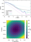 |
Fig. 1. Procedure for finding the correct initialisation of the vertical profile. Top panel: initial (dashed lines) and final (solid lines) vertical metallicity profiles of the mock galaxy. The green line marks the model with the lowest final χ2, while the blue and violet lines correspond to 1σ-worse models. The black line shows the vertical profile of the original mock galaxy. Bottom panel: map of final Δχ2 as a function of initial G and N in Eq. (5). Grey crosses indicate the actually computed models, while the underlying coloured map is a result of interpolation. Red contours depict 1-, 2-, and 3-σ regions. The red cross indicates the model with the lowest χ2. |
The best fit to the mock galaxy profile (i.e. the lowest χ2) is obtained for an initial G = −0.23 dex kpc−1, while the other two models correspond to 1σ worse cases; see lower panel of Fig. 1. The blue line in fact approximates a constant initial prior. The largest difference between the best-fit profile and the other models within the 1σ region is considered as a part of the final uncertainty. In the bottom panel of Fig. 1, we show a Δχ2 map of the models as a function of G and N. We stress again that the exact values of G and N are not directly related to the final vertical profile.
We checked the impact of the vertical prior on the radial profile and it turned out that in the central part it is rather minor. In the outer part, it is more noticeable, which is reflected in a wider uncertainty band for the radial profile beyond R ∼ 7 kpc. In all these tests, the prior did not depend on radius. In Appendix B, we show the effect of initial priors with a radial gradient. We find that the optimal radial gradient is consistent with zero and varying it within the 1σ region has minor impact on the recovered radial profile.
In Fig. 2, we present the mock data, the map of mean metallicity from the best model, and the standardised residuals of the fit. The reduced  indicates an almost perfect fit, which can be also gleaned from the residual plot. However, such a good result is not surprising since the dynamical model is correct and the uncertainties of the data are perfectly Gaussian, with known amplitudes. We conclude that our procedure does not have any persistent problems fitting any of the major features of the mock data.
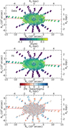 |
Fig. 2. Comparison of the model fit to the mock data. Top: mock map of mean [Fe/H] with a noise of σ[Fe/H] = 0.04 dex. Middle: best M2M dynamical model. Bottom: standardised residuals. The solid red line marks the position angle of the projected disc major axis, while the red arrows mark the orientation and the extent of the bar. |
Let us now compare results of the fitting with the original model. In Fig. 3, we compare various profiles computed both from the original model of Portail et al. (2017b) and our best-fitting M2M model. In the top panel we plot the [Fe/H] profile as a function of cylindrical radius R. We took into account all stellar particles with |z| < 3 kpc. In the second panel we plot the vertical profile for all particles R < 5 kpc. In the last panel, we present the azimuthal profiles for the particles with R < 5 kpc and |z| < 3 kpc.
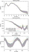 |
Fig. 3. Metallicity profiles calculated from the model fitted to M 31-like mock data (violet, with a grey band of uncertainty), compared to profiles of the original model (green). The yellow lines show profiles resulting from a model fit to spatially-extended mock data. From top to bottom: radial profile (as a function of cylindrical radius), vertical profile, and azimuthal profile. |
Our modelling routine is able to recover all of the features of the radial profile, including the [Fe/H] peaks at ≈1 kpc and close to the end of the bar at ≈3 kpc, as well as a further negative gradient up to 10 kpc. At first sight this might be surprising, since the data along the major axis reach only 5 kpc, however the key lies in the fields along the minor axis, which reach large distances due to the projection at the inclination of 77°. In the azimuthal profile, the main variation is related to the enhancement along the bar, which is aligned with φ = 0, ± π.
As we could already see in Fig. 1, the vertical profile is not reproduced exactly. However, we are able to recover an average vertical gradient. One can also infer a certain degree of non-linearity in the profile, which is flatter closer to the galaxy plane than at larger heights. In Appendix A, we show similar results as in Fig. 3 but for a lower inclination model (i = 45°). Deprojection degeneracies are stronger in this more face-on case, as is apparent particularly in the larger deviations of the recovered vertical profiles from the input model profile.
We carried out another test to judge if the vertical profile is influenced by limited on-sky data coverage. We constructed a complete data set similar to Fig. 2, filling the whole 6 by 12 kpc field. To construct the Voronoi tessellation we used the package VORBIN by Cappellari & Copin (2003). However, for technical reasons2 we used four times fewer Voronoi cells. The yellow lines in Fig. 3 depict the result of modelling these data. The vertical profile is closer to the original model (green line) especially for z > 2 kpc. The radial profile provides a slightly worse match at R ≈ 4 kpc, but much better for R > 4.5 kpc, and the azimuthal profile remains with similar deviations from the true profile.
Therefore, some discrepancy remains even for spatially complete data. This could be ascribed to other causes, such as the orbital degeneracy discussed in the next subsection, the lower spatial resolution, or the noise in the data. It may be surprising that the recovery of the vertical profile in case of an almost (77°) edge-on galaxy is problematic. However, we recall that our earlier tests showed that the constraints on the vertical profiles in more face-on galaxies are much weaker. Furthermore, the vertical variation leaves rather small imprints in an on-sky map, which can be dwarfed by radial changes.
Our estimate of the uncertainties seems to be justified in that the recovered profiles generally are no farther than 1 − 2σ away from the true profiles. On the other hand, the uncertainty in the vertical profile at small heights (z ≲ 1 kpc) appears to be underestimated. We note that errors within a single profile and between different spatial profiles are highly correlated. First, the model is subject to degeneracy due to the galaxy being projected on the sky. Secondly, as the building blocks of our M2M model, we are using spatially-extended orbits, which make a contribution in many different locations.
3.3. Discussion of the method
A valid question would demand what this method can, in fact, constrain, using maps of mean ΦD value on the sky. First, we recall how we may understand the nature of M2M dynamical models that we use as a basis for our work. They are composed of a set of particles in a dynamical equilibrium. However, they can be also regarded as a collection of orbits. Each orbit has an associated mass (equal to the mass of the particle) and the sum of the orbital masses gives a density distribution, whose potential generates the aforementioned orbits. This interpretation resembles the Schwarzschild (1979) modelling, which was used by Long & Mao (2018), Poci et al. (2019), and Zhu et al. (2020) to study stellar populations. We note that Long (2016) implemented a similar technique, however, it was applied to absorption line strengths, limited to symmetrised data and not tested beyond convergence to an acceptable χ2.
If we regard our system as a collection of orbits {i}, then we are actually fitting the mean values of a population parameter on a given orbit. However, we cannot constrain a distribution function of the parameter on the orbit, for example, whether it is δ-like or very broad. Therefore, we also cannot derive the distribution function of ϕ for the whole galaxy, we can only give a rough lower limit on its width. As an extreme example, we might imagine that a spatial map of a galaxy is constant everywhere and equal to ϕ0. We would then conclude that the mean value on all of the orbits is also equal to ϕ0. However, in reality, on each orbit, there might be two stars – one having ϕ = ϕ0 + Δ and the other one with ϕ0 − Δ. Using only the map of the mean value, it is not possible to determine Δ. Having constrained the mean values of ϕ on the orbits, we can project these quantities as a function of more accessible variables, such as spatial coordinates or velocities. In particular, with regard to this contribution, we are focusing on profiles as a function of position, as well as on deprojected maps, but we could also plot ϕ as a function of velocity coordinates or actions.
Thus, our method, or any similar method using the same type of data, naturally produces a distribution function of ϕ at a given position, which reflects the distribution of the ϕ values on the orbits that pass through this position, but it does not necessarily reflect the true distribution of ϕ there. Some progress could be achieved by adding physically-motivated assumptions; for example, Zhu et al. (2020) employed a prior based on an age-orbital circularity relation. In the present context, a natural choice would be a prior relating [Z/H] and [α/Fe]; however, our M 31 data do not show any substantial relation between both quantities. The other, preferred way to improve the recovery of the true distribution of stellar labels would be to use more data constraints, such as those drawn from a full spectral fitting (see e.g., Peterken et al. 2020, Fig. 1).
Another natural question that arises is related to possible degeneracies between stellar orbits. Our method is, in fact, based on matching the projected surface density of ϕ-values on the particle orbits to the data values. If a projection of an orbit could be linearly decomposed into projections of other orbits, then our technique would not be able to unambiguously assign stellar population labels to them. In principle, we expect to see such an occurrence since the orbital phase space can be labelled by three actions (see e.g., Binney & Tremaine 2008), while our data is inherently two-dimensional.
It is relatively easy to understand the issue for axisymmetric disc galaxies. In this case, the orbits can be classified based on three conserved actions. The angular momentum L (equivalent to the azimuthal action) describes the size of the orbit. The radial action Jr refers to the orbital eccentricity. The vertical action Jz describes the vertical thickness of the orbit. We start out by considering only planar orbits (i.e. Jz = 0). In this case the projected density distribution of an orbit with non-zero Jr can be constructed as a sum of density distributions of circular orbits. However, if we project a vertically extended, axisymmetric orbit (with non-zero Jz) at an intermediate inclination, it will appear more extended along the minor axis of the galaxy than a planar orbit of the same radial extent. Therefore, it appears that the Jz dimension is independent of the other two.
The case of barred (i.e. non-axisymmetric) galaxies is more complicated. On the one hand, we still expect some degeneracy because of the difference in the number of dimensions between the phase-space and the data, respectively. On the other hand, neither the classical planar orbital families x1–x4 (Contopoulos & Papayannopoulos 1980), nor the vertically extended orbital families (Skokos et al. 2002), nor the orbits from the actual N-body simulations (e.g., Valluri et al. 2016; Gajda et al. 2016) exhibit obviously degenerate orbital projections. This issue certainly warrants further investigation.
In addition, some of these degeneracies would be reduced with more detailed data, or when such data is lacking, by including additional priors in the modelling. As mentioned above, such priors could include relations between the stellar population labels themselves, such as metallicity and α, or when available, age, or priors with an explicit dependence on the orbital parameters, such as circularity or actions. The drawback with this approach is the difficulty of distinguishing the prediction of the model from that which is simply a corollary of the assumed relations.
The practical conclusion from our mock tests, and similarly based on the findings of Zhu et al. (2020), is that despite the remaining degeneracies, there is considerable information that we can derive from spatially resolved mean maps of stellar population parameters. We showed that the radial and azimuthal profiles are well-constrained and that in nearly edge-on systems, it is possible to retrieve the vertical profile as well when applying some extra care.
3.4. M31 dynamical model and parameters used in stellar population modelling
As the basis for our stellar population fitting, we employed the JR804 N-body model of the Andromeda Galaxy constructed by Blaña Díaz et al. (2018, see Table 1). It consists of 2 × 10⁶ dark matter particles with Einasto density profile, 106 disc particles (which include the bar and its B/P bulge), and 106 classical bulge particles. Using the M2M technique, it was fitted to the moments of the velocity distribution derived by Opitsch et al. (2018) and to the 3.6 μm-band surface brightness maps from the Spitzer Space Telescope obtained by Barmby et al. (2006).
Blaña Díaz et al. (2017, 2018) concluded that M 31 is a barred galaxy. They found that the bar position angle (in the plane of its disc) with respect to the line of nodes is equal to 54.7°. The bar rotates with a pattern speed of Ωp = 40 ± 5 km s−1 kpc−1 and has length of ≈4 kpc. The dark matter halo was found to follow an Einasto profile with a mass of  within 3.2 kpc and a stellar mass-to-light ratio in the 3.6 μm band of
  , assumed to be a single constant. In their work, Blaña Díaz et al. (2018) provide a set of models that fit the data well and which could be thought of as ‘1σ models’. We use those models as a basis for the computation of the uncertainty induced by the variation of the dynamical model.
The M2M model of the Andromeda Galaxy from Blaña Díaz et al. (2018) was fit to a range of observational data and reproduced them correctly. While it did not explicitly fit the vertical scale height, it was based on a model survey by Blaña Díaz et al. (2017), who tested various configurations. Hence, the model’s mean scale height of 0.72 kpc is comparable to the hz = 0.86 ± 0.01 kpc, which can be inferred from the PHAT survey (Dalcanton et al. 2015, see also Bhattacharya et al. 2019). Blaña Díaz et al. (2018) also included a dust model to screen material behind the disc plane of M 31.
Having a detailed dynamical model is an excellent basis for the modelling in this paper since the stellar orbits are thereby determined consistently with the photometry and kinematics. However, some uncertainties remain. We assume that the population labels are mass-weighted and, hence, their best-fit distribution depends on the density distribution. Blaña Díaz et al. (2018) fitted the 3.6 μm IRAC image that traces the old giant stars (the bulk of the population). While the fitting was luminosity-weighted, the assumption of using a single constant mass-to-light ratio implies a trivial relation between particle masses and their 3.6 μm luminosity weights, which, in turn, implies that both mass- and light-weighted averages give exactly the same result.
However, the measured kinematics are light-weighted in the V band where younger or more metal-poor stars could have a bigger impact in some regions (see e.g., Portaluri et al. 2017). Thus, while the surface mass distribution is well-constrained by the infrared photometry, the distribution of the particle orbits is biased towards the V band kinematics without considering the V band photometry. This could be a significant effect in the disk regions with more recent star formation. A future M2M model might be improved by fitting the V-band simultaneously with the IRAC 3.6 μm to better model the kinematic structure in these regions.
An observant reader would notice a small inconsistency in our approach. The dynamical model of Blaña Díaz et al. (2018) assumes a constant M/L, whereas here we determine a posteriori a distribution of metallicities and α-enhancements which should lead to slight variations of the M/L between different parts of the galaxy. The reasoning behind deciding not to vary M/L was our uncertainty as to whether the stellar population labels are precise enough to constrain the dynamics. Additionally, the projected variability of [Z/H] is on the order of 0.2 dex, which implies a difference in the 3.6 μm-band M/L of about 5% (Meidt et al. 2014) and about 10% in the V-band (Vazdekis et al. 2010), both of which are of the same order as the ∼4% uncertainty of our model’s M/L3.6 μm (including a systematic uncertainty from different choices of the dark matter profile). We conclude that the impact of a variable M/L is rather small and does not influence our main results.
As a side note, we remark that to date none of the dynamical models of stellar populations in galaxies is proven to be fully internally self-consistent. Concerning the model of Poci et al. (2019), the remaining question is whether the mass distribution inferred from the orbital light-weights and their respective mass-to-light ratios reproduces the deprojected stellar mass distribution used to generate the orbits. Portail et al. (2017a), Poci et al. (2019), and Zhu et al. (2020) use a single number to convert from an observed quantity to mass (M/L in Poci et al. 2019; Zhu et al. 2020; ‘mass-to-clump ratio’ in Portail et al. 2017a). It appears that actually making a fully self-consistent model is a worthwhile goal for a future research. This should not be too difficult in the M2M: during the iterative joint modelling of the dynamics and the stellar population parameters, the M/L of all particles would be adapted on the fly according to their current ages, metallicities, and α enhancements. However, this would require significantly more detailed data than available here.
Following Blaña Díaz et al. (2018), we set 1 iteration to 1.18 × 10⁻⁴ Gyr. Similarly, we fix the smoothing time scale to τ = 1.6 × 10³ it, which corresponds to the orbital timescale at R = 5 kpc. We tested different values of ϵ that controls the strength of the force-of-change in Eq. (4). We found that in the case of [Z/H] the best results (i.e. the lowest χ2) are obtained for log10ϵ = −1.9 and in the case of [α/Fe] for log10ϵ = −2.1. We smooth the observables initially for 3 × 10³ it, we fit for 50 × 103 it, until χ2 converges to a constant value and then we let the system relax for 7 × 10³ it. As usual in the M2M modelling, after we finish fitting χ2 increases in the relaxation phase by about  , and stabilises at a new and final value.
4. Results
4.1. M 31 metallicity
First, we present our modelling of the [Z/H] distribution in Andromeda. Similarly as in the mock test, we use a vertical initial prior with parameters (G, N), finding that G = −0.21 ± 0.27 dex kpc−1 and N = −0.02 ± 0.16 dex result in the models with lowest overall χ2. In Fig. 4 we show the data (top), the best model (middle) and the standardised residuals (bottom). The white spaces correspond to the lines-of-sight not covered by the data. The (Rx, Ry) reference frame (the same as in Blaña Díaz et al. 2018) is rotated by 50° clockwise with respect to the sky coordinates, so that the projected major axis of the M 31 disc is almost aligned with the Rx-axis. The kpc labels correspond to the sizes on the sky at the distance of M 31. To convert Ry into a distance in the plane of the disc, it should be multiplied by (cos i)−1 ≈ 4.4; thus, the elliptical region on the sky covered densely by the data fields extends to 5.5 kpc along the minor axis. We also note that the data cover nearly the entire bar length. The possible values of [Z/H] are limited to the range −2.25 to 0.67 dex, as in Saglia et al. (2018).
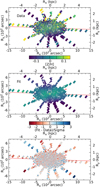 |
Fig. 4. Metallicity maps of the Andromeda Galaxy. Top: map of the measured [Z/H]. Middle: best model. Bottom: standardised residuals. The solid red line marks the position angle of the projected disc major axis, while the red arrows mark the orientation and the extent of the bar. |
Overall, the data are fitted very well by the model ( ), especially in the central parts. However the fit appears to be worse for some of the high values in the spokes (Ry > 300″) covering the disc, where [Z/H] is underestimated. The data itself exhibit a significant asymmetry, with the top part of M 31 having higher metallicity than the bottom part (see top panel of Fig. 4). This could be related to dust obscuration by the disc whose nearby parts are in front of the bulge at Ry > 0 (see Blaña Díaz et al. 2018, Sect. 3.2.3). In Appendix C, we discuss, in greater detail, the arguments that the dust is at least partially responsible for the asymmetry.
In Fig. 5, we present the metallicity profiles for M 31, calculated from the best model. We plot [Z/H] as a function of cylindrical radius R (i.e. measured in the plane of the disc), height above the disc plane z, and azimuthal angle φ. We took into account only the particles with |z| < 3 kpc. For the vertical profile, we used particles with R < 5 kpc, and for the azimuthal profile, we took into account only particles with R < 5 kpc and |z| < 3 kpc.
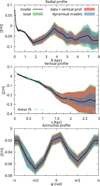 |
Fig. 5. Metallicity profiles calculated from the best model. From top to bottom: radial profile (as a function of the cylindrical radius), the vertical profile, and the azimuthal profile (black lines). The coloured bands show the different uncertainties. In red we mark the sum of the errors stemming from the uncertainties in the data and the vertical profiles, in blue we show the error range resulting from the uncertainty of the underlying dynamical model, and the green bands mark our final uncertainty estimates, which are the sum (in quadrature) of the three. We note that overlapping red, blue, and green appears as grey, and overlapping red and green as orange. Middle panel: the turquoise dashed line represents an uncertainty-weighted linear fit to the model curve. |
For each profile we mark the different uncertainties. The red bands include the uncertainty stemming from re-fitting the model to different realisations of the data within their errors and from using different priors for the vertical profile within their respective 1σ uncertainties. Blue bands show the uncertainty range from the dynamical model, derived from the 11 models in Table 1 of Blaña Díaz et al. (2018), which the authors of this study deemed ‘acceptable’ models. Their dark matter halos all have the Einasto density profile, but they differ somewhat in the bar pattern speed, mass-to-light ratio, and dark matter mass in the bulge region. We refitted the M 31 metallicity observations for all these models with the same initial vertical profile as in our fiducial case. We inspected the resulting models of the [Z/H] distribution and they were qualitatively similar to the case of the fiducial dynamical model. To assess the quantitative differences, we computed the dispersion of these profiles with respect to the fiducial model and plotted it as the blue bands in Fig. 5. This uncertainty has a similar if slightly smaller magnitude as the other types of uncertainty, except at large heights where the uncertainty from obtaining the vertical profile dominates. Finally, the green bands in Fig. 5 depict the overall uncertainty of our model, where we added in quadrature all three sources of error.
In the radial profile, we immediately notice a spike in the central ∼200 pc, which is also discernible in the raw data of Saglia et al. (2018, in Fig. 22), and was interpreted there as a sign of the classical bulge. Then [Z/H] decreases further, up to ≈2 kpc, which we interpret below in terms of the metallicity desert perpendicular to the bar. Further out, the azimuthally averaged profile starts to increase again, reaching a maximum around 4 kpc from the centre. This coincides with the size of the bar in the model of Blaña Díaz et al. (2018). Still further out, in the disc outside the bar, the profile decreases once again, but does not exhibit a steady negative gradient, possibly due to insufficient data coverage. We limit the radial range of the profile to 8 kpc because the asymmetry of the data (see Fig. 4) strongly influences the results beyond that point. Our profile can be compared to the radial metallicity profile obtained by the PHAT survey (Gregersen et al. 2015). Their radial profile has a metallicity maximum at R ≈ 4.5 kpc and further away [M/H] decreases linearly with radius. While we do not find a clear linear decrease beyond the end of the bar, our mean values are consistent with the median values reported in their Fig. 9.
The azimuthal profile supports the conclusion by Saglia et al. (2018) that [Z/H] is enhanced along the bar (aligned here with φ = 0, ± π). The [M/H] map by Gregersen et al. (2015) also indicates that metallicity is enhanced along the bar, particularly close to its tip.
The average vertical profile is consistent with linearity. Thus, we fitted a linear function using uncertainty-weighted least squares and obtained a vertical gradient of ∇z[Z/H] = −0.133 ± 0.006 dex kpc−1 (see Fig. 5). We note that the uncertainty of the slope is likely underestimated since it is driven by the well-constrained region at |z| < 1 kpc.
In our Fig. 6, we show deprojected maps of the mass-weighted mean metallicity. The minor axis of the disc is aligned with the z-axis, while the bar major axis is here aligned with the x-axis. To create these maps we used only the particles within R < 7.2 kpc and |z| < 3 kpc. Then they were time-smoothed in the frame rotating with the bar using Eq. (2), with a time-scale of τ = 0.19 Gyr. To guide the eye, the surface density contours are overplotted in black.
 |
Fig. 6. Deprojected maps of mass-weighted mean [Z/H] in M 31. From left to right: face-on, edge-on and end-on view. Surface density contours are overplotted in the range of log(Σ/(M⊙ kpc−2)) = 8 − 10, with a multiplicative step of 101/3. |
In the central 3 kpc of the face-on view, we can see an enhancement along the bar and depressions in the direction perpendicular to it. Further away, we can notice maxima at both ends of the bar, around x ≈ 4 − 5 kpc. There is also a noticeable asymmetry between positive and negative y, from |y|∼4 kpc outwards, with a larger metallicity inferred at positive y. This is a direct consequence of the top-bottom asymmetry of the data (Fig. 4). We checked that this feature is dynamically stable, continuing the relaxation phase for 5 × 10⁴ it (≈6 Gyr). In Appendix C, we describe additional tests related to this asymmetry which indicate that orbits around the Lagrange points L4/L5 make it dynamically stable. Thus, in principle, the [Z/H] distribution itself could by asymmetric in M 31, for instance, due to enhanced star formation in spiral arms on one side of the galaxy. However, we cannot currently discriminate whether the inferred larger [Z/H] at large positive y (see top panel of Fig. 4), are caused by the dust or whether they are due to intrinsic asymmetry of M 31. Therefore, we consider the bottom part of the map (y < 0) more trustworthy. It exhibits a noticeable ring of enhanced metallicity, beyond which [Z/H] decreases outwards, compatible with Gregersen et al. (2015).
The edge-on view clearly exhibits an X-shape. The obvious explanation for this appearance would be the B/P bulge, however, the X-shape extends much further, well into the disc. To investigate this further, we show in Fig. 7 [Z/H] profiles along the major axis of the bar at different vertical heights. Only particles within |y| < 1 kpc are included (y is along the bar intermediate axis). The profile in the midplane of the model (|z| < 0.33 kpc) is roughly flat up to ∼3 kpc and rises further out. The second [Fe/H] profile shows the B/P region (0.33 < |z| < 1.0 kpc), growing from the centre outwards, reaching its maximum at x ≈ 2.5 kpc, and then declining along x further out. This particular behaviour coincides with the extent of the B/P bulge (see the density contours in the middle panel of Fig. 6 and also Blaña Díaz et al. 2018, Fig. 19), which has a length of about 2.5 − 3 kpc and a height of about 1 kpc. The third profile corresponds to the part of the model above the B/P bulge (1.0 < |z| < 1.67 kpc). In this slice [Fe/H] grows from the centre outwards, reaching the largest values at x ≈ 4.5 kpc. All three profiles combined show that the vertical [Z/H] profile at x ≈ 2 − 3 kpc (the end of the B/P bulge) is effectively flat up to z ≈ 1 kpc and declines at larger heights. This demonstrates that the B/P bulge significantly affects the metallicity distribution in the centre of M 31.
 |
Fig. 7. Metallicity profiles in three adjacent horizontal strips in the central region of M 31. The B/P bulge extends to x ≈ 2.5 − 3 kpc and z ≈ 1 kpc, while the bar length is ∼4 kpc. The maximum along the second (green) [Fe/H] profile corresponds approximately to the end of the B/P bulge. |
Clearly, the flaring of the [Z/H] distribution further out is unrelated to the B/P bulge. It is possible that the metal-rich disc of M 31 was thickened due to the recent merger inferred from the age-velocity dispersion relation of the disc (Bhattacharya et al. 2019). In the end-on view (the right panel of Fig. 6), the most prominent feature is the asymmetry with respect to the y = 0 kpc line, which we discussed above.
To further investigate the relation of [Z/H] and the bar, we split the stellar particles into two groups, using a very simple criterion. We considered as bar-following all the particles on elongated orbits, defined as |y|max < 0.7|x|max and |x|max < 4 kpc, where | ⋅ |max denotes the maximum absolute excursion along either major or intermediate axis of the bar (in the rotating bar frame). The first condition ensures that the orbits are elongated rather than circular, and the second that we only consider the particles that do not leave the bar area. In the second, non-bar-following group we included all the other stellar particles, that is, those on more circular orbits in the bar region as well as those in the outer disc. Here, we do not distinguish between the disc particles and the classical bulge particles. In Fig. 8, we show the metallicity distribution of the two groups in the face-on view (in the bar frame) and in the meridional plane (R, z). We show only the pixels where a given component is present and the uncertainty is not too high, that is, σ[Z/H] < 0.2 dex. The latter concerns mostly the bar-following component close to the z-axis, due to its low density in that area. Similarly to Fig. 6, the maps were time-smoothed with τ = 0.19 Gyr.
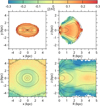 |
Fig. 8. Metallicity distribution of the bar-following orbits (top row) and the non-bar-following orbits (bottom row) in the face-on view (left column) and in the meridional plane (right column). The surface density contours are overplotted in the ranges of log(Σ/(M⊙ kpc−2)) = 7 − 9.5 (top row) and 8 − 10 (bottom row), in both cases with a log-step of 0.5. |
The bar-following orbits are significantly more metal-rich than the second group, supporting our conclusion that the bar is more Z-enhanced. The bar ends stand out as especially metal-rich, where [Z/H] reaches ∼0.2 − 0.25 dex, and we believe this is a robust prediction of our model. On the (R, z) plane the B/P bulge causes a vertical flaring of metallicity.
The non-bar-following population also flares, but beyond the bar end, more data with extended spatial coverage is needed to establish this more firmly. The previously discussed metallicity deserts perpendicular to the bar appear to be due to more metal-poor stars on nearly axisymmetric orbits in a radial range of about R ∼ 1.5 − 2 kpc. In the innermost 1 kpc, we can take note of a [Z/H]-enhancement of a roughly donut-like shape, which could be caused by additional star formation and enrichment in a nuclear ring.
4.2. Enhancement of [α/Fe] in M 31
We now focus on the [α/Fe] enhancement, which provides a signature of star-formation timescales (e.g., Tinsley 1979; Matteucci & Greggio 1986; Ferreras & Silk 2002; Thomas et al. 2005), that is, larger α-enhancement signals quicker star formation. We construct separate models for the [α/Fe] distribution, that is, the model of the α-enhancement is not influenced by the metallicity model, they only share the common underlying dynamical model. As before, for metallicity, we plot in Fig. 9 the data from Saglia et al. (2018), our best-fit model, and a map of standardised residuals. Overall,  , indicating a good fit. There are no correlations apparent in the distributions of positive and negative residuals. The possible values of the particle [α/Fe] in the model are limited to the range from −0.3 to 0.5 dex, as in Saglia et al. (2018). As before, we tried a range of initial vertical profiles (see Eq. (5)). The preferred values of G, N and the respective 1σ ranges were determined similarly as for the mock data, resulting in G = 0.16 ± 0.41 dex kpc−1 and N = 0.42 ± 0.20 dex and a corresponding error range for the final model.
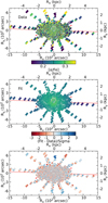 |
Fig. 9. Map of [α/Fe] enhancement in the Andromeda Galaxy. Top: measured [α/Fe]. Middle: best model. Bottom: standardised residuals. The solid red line marks the position angle of the projected disc major axis, while the red arrows mark the orientation and the extent of the bar. |
At first glance, we can see from these maps that the centre of M 31 is relatively more α-enriched and the shape of this feature is elongated along the projected minor axis of the galaxy. This is because the lower-α bulge material is elongated along Rx (see Saglia et al. 2018). Furthermore, [α/Fe] seems to decrease along the projected major axis for |Rx| > 2 kpc, but is quite flat in the Ry direction.
Profiles of [α/Fe], calculated from our best M2M model, are shown in Fig. 10, as a function of the cylindrical coordinates R, z, and φ. Here, we took into account only those particles within |z| < 3 kpc. For the vertical profile, we integrated over the region R < 5 kpc, while for the azimuthal profile we considered only the region R < 5 kpc, |z| < 3 kpc. As in the case of [Z/H] profiles, we plot different types of the uncertainty bands. In red, we show the sum of the errors due to the data uncertainties and the range of initial vertical profiles. In blue, we depict the uncertainty due to the underlying dynamical models, which is subdominant with respect to the other two, and in green, we show the overall uncertainty of the model profiles.
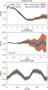 |
Fig. 10. Profiles of the α-enhancement, calculated from the fitted model. From top to bottom: radial profile (as a function of the cylindrical radius), vertical profile, and the azimuthal profile. Coloured bands show the different uncertainties as in Fig. 5. Middle panel: the turquoise dashed line represents an uncertainty-weighted linear fit to the model curve. |
In the inner 1.5 kpc, the radial profile is rather flat, then it decreases to a minimum at R ≈ 4 kpc. Further out, the profile gently bends upwards, however, it is still consistent with a constant value. Recall that the data with good spatial coverage extend to deprojected R ∼ 5.5 kpc, along the minor axis. The drop in the innermost ∼300 pc can be attributed to the presence of a young stellar population (Saglia et al. 2018). It is worth noticing that the data are consistent with the inner disc of M 31 having super-solar α-enhancement, and, hence, short star-formation timescale (Thomas et al. 2005). Conversely to the metallicity, in the azimuthal profile, [α/Fe] is higher in the direction perpendicular to the bar, suggesting that some stars in the bar formed later than the stars in the inner disk.
We made a linear fit to the vertical [α/Fe] profile and obtained a value of ∇z[α/Fe] = (−0.005 ± 0.003) dex kpc−1. Judging from the error band, [α/Fe] is consistent with constant in the direction perpendicular to the disc, at least on average in the inner 5 kpc.
In Fig. 11, we show deprojected maps of the mass-weighted mean α-enhancement. Similarly to Fig. 6, the bar major axis is aligned with the x-axis and the disc rotation axis coincides with the z-axis. As before, the maps were time-smoothed following Eq. (2).
 |
Fig. 11. Deprojected maps of the mass-weighted mean [α/Fe] in M 31. From left to right: face-on, edge-on and end-on view. The surface density contours are overplotted in the range log(Σ/(M⊙ kpc−2)) = 8 − 10 with a multiplicative step of 101/3. |
In the face-on view, the orientation of the [α/Fe] enrichment is clearly perpendicular to the bar direction and coincides with the metallicity deserts discussed in the previous subsection. The face-on map exhibits a lower-α ring at R ∼ 3 − 4 kpc, signalling additional late enrichment, which is coincident with the metallicity enhanced ring visible in the bottom part of the left panel of Fig. 6.
In the central parts of the edge-on and the end-on view the enhancement is high, with small-scale patterns which may or may not be real. The high [α/Fe] are most probably related to the classical bulge and the regions where it dominates over the disc population. Further out, the increase to higher [α/Fe] in the X-shaped pattern in the edge-on view is spatially approximately coincident with the decrease in metallicity outside the B/P bulge; see Fig. 6. In the outer part of the disc, the α-enhancement is smaller closer to the disc plane and grows with height. This trend can be interpreted as an indication of the presence of an α-rich thick disc.
Similarly to the metallicity, we also traced the α-enhancement distribution of the bar-following (|y|max < 0.7|x|max and |x|max < 4 kpc) and the non-bar-following (remaining) stellar particles. In Fig. 12 we show their [α/Fe] maps in the face-on projection and in the meridional plane (R, z). We plot only the pixels where a given component is present and where the uncertainty is not too high, that is, σ[α/Fe] < 0.15 dex. The latter concerns mostly the bar-following component close to the z-axis. As in the previous instances, the maps were time-smoothed with τ = 0.19 Gyr.
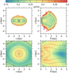 |
Fig. 12. Distribution of [α/Fe] enhancement of the bar-following orbits (top row) and the non-bar-following orbits (bottom row) in the face-on view (left column) and in the meridional plane (right column). The surface density contours are overplotted in the ranges of log(Σ/(M⊙ kpc−2)) = 7 − 9.5 (top row) and 8 − 10 (bottom row), in both cases with a log-step of 0.5. |
In the face-on map, the most elongated orbits, close to the major axis of the bar, have somewhat lower [α/Fe], which could be linked to younger ages (see simulations analysed in Fragkoudi et al. 2020). This would also influence the B/P bulge and, correspondingly, the bar-following orbits in the meridional plane appear to have slightly lower α-enhancement than the non-bar orbits in the inner 2 kpc, by ∼0.1 dex. We consider the increase in [α/Fe] in the outer envelope of the bar-following population possible, but we must keep in mind that the uncertainty in this region is higher, chiefly due to the lower density of this component in this region.
In the non-bar population, we can see the low-α ring at R ∼ 4 kpc, which has also elevated [Z/H]. The α-rich region at R ∼ 1.5 kpc is related to the metallicity desert. Further in, at R ∼ 1 kpc, the model has a possible quasi-spherical shell with relatively lower α. It is unclear what the significance of this feature is, but it corresponds to a higher-metallicity feature in the same region and there is a possible (noisy) lower-α circular feature in the data at R ∼ 250 arcsec (top panel of Fig. 9) that could cause it. If this shell feature is real, the most plausible explanation would be that it is due to accreted material, but confirming this requires further investigation.
5. Discussion
5.1. Comparisons with Saglia et al. (2018)
Several features of the stellar population distribution in M31 were clear from an inspection of the maps obtained by Saglia et al. (2018), such as the [Z/H] enhancement along the bar and the [α/Fe] peak in the central 1 kpc. In addition, Saglia et al. (2018) constructed a simple decomposition of their stellar population data into various components (classical bulge, B/P bulge, bar, and disk), which was based on using different regions of the sky to constrain the classical bulge and bar components in the mass model of Blaña Díaz et al. (2018).
It is useful to compare our detailed results to the mean profiles of their model (blue and black lines in Figs. 21–24 of Saglia et al. 2018). We found a steep increase in metallicity and steep decrease in [α/Fe] in the inner 200 pc (50″), which was directly mandated by the data we used. Saglia et al. (2018) ascribed the [Z/H] peak to the classical bulge, while the α decrease was attributed to the recent star formation. We agree with the Saglia et al. (2018) model that along the bar metallicity is constant, while [α/Fe] decreases. These authors found almost flat metallicity profiles for the B/P bulge and the disc (Figs. 23 and 24). Our model shows that the B/P bulge has an X-shape in [Z/H], as can be found in Fig. 6. Thus, the metallicity profiles in the B/P bulge grow with radius, up to its end at ≈2.5 kpc, at a range of heights at z ∼ 0.3 − 1 kpc. The [Z/H] morphology of the disc shows diverse features: metallicity deserts perpendicular to the bar at |y|∼2 kpc, then further away an enriched elongated ring at R ∼ 3 − 5 kpc and a possible further decrease beyond 5 kpc. The vertical distribution of [Z/H] beyond the B/P bulge seems to be flaring. Our [α/Fe] distribution in the central part of M 31 show enhancement perpendicular to the bar and up to a significant height. Our model shows a steeper α-overabundance decrease up to R ∼ 4 kpc than in Fig. 24 of Saglia et al. (2018).
It would be tempting, at this point, to perform a decomposition into classical bulge, B/P bulge, bar, and disk components, using the model by Blaña Díaz et al. (2018) that explicitly consists of two types of particles (belonging to the classical bulge and disc). However, because of the spin-up through angular momentum transfer by the bar (Saha et al. 2012, 2016), some of the classical bulge orbits overlap with those of the bar. Our current method cannot differentiate between the mean metallicities of the two components on the same orbit. From our final model, we can only tentatively say that the bulge component has a very steep gradient, while the profile of the disc component (which contains the bar) is flat or even decreasing towards the centre, however we are not able to give the uncertainties. The classification of the stellar particles as bar-following and non-bar-following, presented in Figs. 8 and 12, should not be taken as a proxy for a decomposition into the classical bulge and the combined bar and B/P bulge, due to the aforementioned spin-up of the classical bulge and overlap of orbits. Improving this aspect of the model seems possible but it is beyond the scope of this paper.
Compared to the earlier modelling, several new qualitative results have emerged from our full particle modelling of the stellar population data: the discovery of a metallicity X-shape in the edge on-view, caused by a metallicity enhancement in the B/P bulge and the further flaring in the disc. Additionally, we found a [Z/H]-enhanced, low-α ring, as well as metallicity maxima at the tips of the bar. Furthermore, we found indications of an α-enhanced thick disc in M 31.
5.2. Comparison with other galaxies
The impact of the bar on the stellar population gradients has been an active topic for some time now. It has been found that the profiles along the bars are flatter than those perpendicular to bars (Sánchez-Blázquez et al. 2011; Fraser-McKelvie et al. 2019; Neumann et al. 2020). Interestingly, the results of Fraser-McKelvie et al. (2019, Fig. 2) indicate that the gradients may be either positive or negative (see also Pérez et al. 2009), but the signs of the gradients in the directions parallel and perpendicular to the bar remain correlated with each other. However, judging from our M 31 results, it is important to go beyond simple linear fitting since the profiles in the bar region can be more complicated. Looking at Fig. 5, it is possible to infer a negative radial [Z/H] gradient in the central ∼2 kpc and a positive one further out, up to the bar end. Seidel et al. (2016), in their Fig. 10, presented a step in this direction, where they found that the slopes of the Mg b index profiles change abruptly at around 10−15% of their bar length.
It appears that the metallicity enhancement close to the bar ends, as we find in our M 31 model, has not yet been widely acknowledged. However, a closer inspection of available spatially resolved data sometimes reveals such trends. Many of the BaLROG bars show this feature (Seidel et al. 2016), as well as some of the galaxies analysed in the TIMER project (Gadotti et al. 2019; Neumann et al. 2020). Moreover, the APOGEE data for the Milky way indicate the presence of a metallicity maximum close to the bar end at l ≈ 30° (e.g., Ness & Freeman 2016). The subsequent maps of Bovy et al. (2019) can be interpreted as that [Fe/H] is either enhanced at the bar end or in a nearby ring. On the other hand, Wegg et al. (2019) found more enhanced metallicities in their bar fields 4 kpc from the centre.
It is also interesting to compare side-on views of our results to other published examples. According to the M 31 models, [Z/H] is enhanced in the B/P bulge and shows signs of flaring further away from the centre, while [α/Fe] is high in the classical bulge region and at large heights above the disc plane. The edge-on galaxy NGC 1381 of Pinna et al. (2019a) shows clear signs of a B/P shape both in terms of the metallicity and [Mg/Fe]. Williams et al. (2011) suggested that this galaxy may have a small classical bulge, which would make it different from M 31 with its sizeable classical bulge. Pinna et al. (2019b) studied another galaxy with a B/P bulge, FCC 177. However, this one does not have obvious signs of the B/P bulge in metallicity and certainly not in [Mg/Fe]. However, curiously, [Fe/H] seems to have maxima in the disc plane at ≈3 kpc from the galaxy centre, beyond the B/P bulge (of size ∼1.5 − 2 kpc, judging from the isophotes). In the case of the Milky Way the model of Portail et al. (2017b, Fig. 10) suggests that the [Fe/H] distribution in the centre has a peanut-like shape (see also the N-body models of Debattista et al. 2017; Fragkoudi et al. 2018).
In the Milky Way α-enhancement is anti-correlated with metallicity, broadly speaking (e.g., Hayden et al. 2015, and many others). In our model, this is also true to a certain degree. In the face-on view, α-rich regions coincide with the metallicity deserts perpendicular to the bar. The high-[Z/H] ring is relatively less α-enhanced. In the edge-on views, at large distances from the centre, a negative metallicity gradient corresponds to a positive α gradient. Apparently, the centre of M 31 does not follow this trend, presumably due to the metal-rich, high-α classical bulge.
5.3. Origins of the spatial trends
Many of the models aimed at explaining the origin of the stellar populations in disk galaxies are focused on the Milky Way because it is the galaxy that offers the greatest store of detailed data. However, these models are often useful for M 31 as well, since it is a disk galaxy of similar mass and also includes a bar and B/P bulge component. In many cases, authors assume a certain initial metallicity distribution and test the impact of the further secular evolution (e.g., Martel et al. 2013; Martinez-Valpuesta & Gerhard 2013; Di Matteo et al. 2013). The alternative approach is to trace stellar populations in hydrodynamical simulations with star formation and feedback (e.g., Grand et al. 2016; Debattista et al. 2017, 2019; Tissera et al. 2016, 2017, 2019; Taylor & Kobayashi 2017).
Di Matteo et al. (2013) analysed a case where a disc galaxy has initially an axisymmetric distribution of mass and metallicity, with [Fe/H] assigned such that it decreased linearly with the radius. During the subsequent evolution, a bar and spiral arms were formed. The creation of the bar induced outwards radial migration and effectively mixed the stellar metallicities from the galaxy centre up to the bar length, creating an enhancement along the bar and metallicity-deserts perpendicular to it (see also Debattista et al. 2020, Fig. 15). This resulted in an azimuthal variation of metallicity. They found that the ratio of the azimuthal variation δ[Fe/H] (measured, for example, in the bar region, see Di Matteo et al. 2013, Fig. 8 and Sect. 3.3) and the initial metallicity gradient Δ[Fe/H] can be approximated by δ[Fe/H]/Δ[Fe/H] ∼ 1 ± 0.5, independently of the initial gradient. In our case, δ[Z/H] ≈ 0.02 dex (Fig. 5), which would correspond to an initial radial gradient in Andromeda on the order of ∇R[Z/H] ∼ 0.02 ± 0.01 dex kpc−1. This is compatible with the metallicity gradient in the outer disc of M 31 derived from the PHAT survey (Gregersen et al. 2015), but also with typical radial gradients in other galaxies (Sánchez-Blázquez et al. 2014; Goddard et al. 2017; Zheng et al. 2017) and in some hydrodynamical simulations for redshift z < 1 (Tissera et al. 2017). We note that the exact shape of the bar-related enhancement depends on the initial mix of the stellar populations (Khoperskov et al. 2018).
Further work is needed to understand the influence of the purported recent merger on M 31 (Hammer et al. 2018; Bhattacharya et al. 2019), and whether it deposited enough material in the bar region to significantly change the mean stellar population parameters there. Alternatively, the enhancement along the bar may be caused by the so-called kinematic fractionation effect (Debattista et al. 2017; Fragkoudi et al. 2017), by which the population that is colder prior to the bar formation would become more strongly aligned with the bar afterwards. If the colder population was additionally more metal-rich, this would result in a metallicity enhanced bar. In the Milky Way, the more metal-rich populations exhibit distributions that are more strongly barred (Portail et al. 2017b). Moreover, the bar metallicity can be further enhanced during its growth, if the bar can capture new stars that are more metal rich (e.g., Aumer & Schönrich 2015).
For the α-enhancement in M 31, we find only a weak anticorrelation with the bar. The stellar component on the most elongated bar-following orbits is somewhat more α-enhanced than the surrounding disc. The high α value (≳0.15 dex everywhere) implies that the stars in the entire bar region must have formed quite rapidly at early times (Pipino et al. 2006, 2008). The stellar population that formed the bar also appears to not have had an initial [α/Fe] radial gradient, that is, the entire bar and the surrounding disk stars must have formed rapidly at early times. The original galaxy also should not have had multiple discs of different α, such as a distinct α-rich thick disc, since this would probably also result in a bar-related non-axisymmetry (Fragkoudi et al. 2018). The slightly lower [α/Fe] in the bar region could be related to late-time star formation, which is also necessary for the formation of the α-poor ring.
The X-shaped side-on view of the metallicity is an expected outcome of the hydrodynamical simulations, both in isolation (Debattista et al. 2017) and in the cosmological context (Debattista et al. 2019; Fragkoudi et al. 2020). The X-shape in the region of our model’s B/P bulge (|x|≲2.5 kpc) is probably somewhat weaker than in the simulated galaxies, since the dynamical B/P bulge is weaker due to the presence of the classical bulge. Differently from the models, the metallicity distribution in M 31 keeps flaring with growing distance from the centre. The origin of this flare could be related to the heating of the disk caused by the merger inferred to have occurred ∼3 Gyr ago (Hammer et al. 2018; Bhattacharya et al. 2019). On the other hand, the cosmological zoom-in model of Rahimi et al. (2014) also exhibits a positive radial metallicity gradient at large heights. The authors ascribed it to the flaring of the young, metal-rich stellar population in the outer disc. Certainly, more spatially extended data beyond the bar end would help to constrain the model more strongly. The side on-map of [α/Fe] in M 31 looks different from those obtained in the Auriga simulations (Fragkoudi et al. 2020). We note that these Auriga galaxies do not have classical bulges (as inferred from small Sérsic indices), while M 31 clearly has one. We also note that their average [α/Fe] are much closer to the solar value than in Andromeda.
Metallicity enhancement along bars and maxima at their ends are also found in hydrodynamical simulations (Debattista et al. 2019; Fragkoudi et al. 2020). In particular, two of the runs (Au18 and Au23) analysed by Fragkoudi et al. (2020) exhibit both [Fe/H] maxima at the bar ends and rings of enhanced metallicity and relatively lower-α. The authors of that study relate the rings to on-going star formation in the region between the bar end and the corotation radius. The runs Au18 and Au23 are different with respect to the others analysed by Fragkoudi et al. (2020) also in terms of their rotation curves, which are not centrally peaked, similarly to M 31 (Blaña Díaz et al. 2018) and the Milky Way (e.g., Portail et al. 2017a). The Auriga bars are also significantly smaller than their corotation radii, that is, they are relatively slower. The enhancement close to the tip of the bar could be related to the star-formation activity observed there in some galaxies (e.g., Phillips 1996). On the other hand, Debattista et al. (2020, Fig. 15) found that if the particles are tagged with metallicity corresponding to an axisymmetric galaxy and let the galaxy form a bar, then the metallicity becomes enhanced along it, but the maxima at the bar ends do not form. High-metallicity rings and arcs beyond the metallicity desert are also described in Khoperskov et al. (2018), where they are related to spiral arms (see also Debattista et al. 2019, Fig. 8). They arise from stellar populations with different kinematics and metallicity patterns, which respond differently to the spiral arms. The ring we find in our model could, in principle, have a similar origin.
6. Conclusions
In this paper, we devise a new chemodynamical technique based on the made-to-measure (M2M) modelling framework, enabling us to constrain the distribution of galactic stellar populations. As input, the method uses mass-weighted maps of a mean stellar population parameter, for example, metallicity, age, or α-enhancement. We start with a dynamical N-body model, constrained by surface density and kinematics. Then we tag the particles with single values of, for instance, metallicity, corresponding to the mean metallicities along their orbits, and then we adjust those values to match the observational constraints. We tested our method on mock data and found that the radial and azimuthal profiles in the plane of the galaxy are well-reproduced, while in the case of the vertical profile, we are only able to obtain an average gradient, without any finer details.
We applied our technique to the Andromeda Galaxy. We used [Z/H] and [α/Fe] maps derived by Saglia et al. (2018) to constrain the three-dimensional distribution of metallicity and α-enrichment in the context of the M 31 dynamical model of Blaña Díaz et al. (2018). Our main results can be summarised as follows:
-
We find that the metallicity is enhanced along the bar, while perpendicular to the bar, we see a clear depression, akin to the so-called star formation deserts (James et al. 2009; Donohoe-Keyes et al. 2019). The enhancement along the bar is directly related to the high metallicities of bar-following orbits. We also find that the metallicity distribution exhibits a peak at the radius corresponding to the bar size, corresponding in the face-on view to an elongated, [Z/H] enhanced ring.
-
A closer inspection of the side-one view and orbital analysis reveals that the [Z/H] enhancement has an X-shape caused by the boxy/peanut (B/P) bulge. The average vertical [Z/H] gradient in the entire inner region of M 31 is −0.133 ± 0.006 dex kpc−1. This is significantly lower (by about half) than typical values in other galaxies presented by Molaeinezhad et al. (2017) but there are some galaxies with similar vertical gradients in their sample.
-
On average, the [α/Fe] enhancement in Andromeda is high compared to solar, indicating short formation timescales. The centre of M 31 is more α-enhanced than the surrounding disc, likely due to the presence of the classical bulge. We find a relatively lower-α ring, corresponding to the metallicity ring. Some of the most elongated bar-following orbits also have a somewhat lower [α/Fe] than the average. The average vertical [α/Fe] gradient is flat, however a closer look reveals more structure: near the centre α-enhancement decreases slightly while in the disc it increases with height; this may signify a presence of a more strongly α-enhanced thick disc.
From the data of Saglia et al. (2018) and based on our model, the following formation pathway for the Andromeda Galaxy can be deduced. Given the overall high level of α-enhancement, the stars in both the bulge region and the inner disc must have formed relatively quickly, with faster star-formation in the bulge region. Since the current structure of the metallicity and α distributions are qualitatively different, they must have been different initially. The distribution of [α/Fe] is consistent with no radial gradient or any other structure in the original disc. The galaxy assembly resulted in a sharp peak of metallicity in the central few hundred parsecs and a more gentle negative gradient in the remaining disc. The formation of the bar leads to a re-arrangement of the [Z/H] distribution, causing the formation of metallicity-deserts and a flat gradient along the bar. Afterwards, the star formation continued close to the bar ends in the leading edges of the bar, producing metallicity enhancements in the ansae and the [Z/H] enhanced, lower-α ring. Star formation in the very centre, at ∼200 pc, also continued, however it was rather mild, leading to only a small decrease in [α/Fe] there. Andromeda probably experienced recently a fairly massive minor merger (Hammer et al. 2018; Bhattacharya et al. 2019), which most probably led to flattening of the gradients (e.g., Taylor & Kobayashi 2017). It would be interesting to further investigate the impact of a merger on the distribution of the stellar populations in barred galaxies.
In this work, we constrain our models with spatially resolved maps of line-of-sight averages of a given stellar population parameter. Thus, we could only constrain the mean metallicity and [α/Fe] distribution in the corresponding parts of the orbit-space and deprojected space. The obvious way forward is to use separate maps for intervals of metallicity or age from the full spectral fitting, similar to those presented in Peterken et al. (2020, Fig. 1).
Our newly developed technique proved to be a valuable tool for studying the distribution of the stellar populations in galaxies, To date, such analyses have always been confined to looking at galaxies either face-on or edge-on. Here, we are able to model the three-dimensional distribution and thereby connect the results from both perspectives. In the future, we plan to apply our technique to other galaxies with spatially-resolved maps of metallicity, α-enhancement, and age, thereby obtaining a more complete picture of the chemodynamical structures in disk galaxies.
Here, we recall that in dynamics there are three basic dimensions, which can be chosen as, for example, length, velocity, and mass. The gravitational interactions are invariant under the transformation x → αx, v → βv and m → αβ2m, where x denotes coordinates, v denotes velocities and m denotes masses. We note that due to this transformation time t → (α/β)t.
Acknowledgments
We would like to thank Chiara Spiniello for useful discussions about stellar population measurements and the anonymous referee for constructive comments. The research presented here was supported by the Deutsche Forschungsgemeinschaft under grant GZ GE 567/5-1. The research presented here is partially supported by the National Key R&D Program of China under grant No. 2018YFA0404501; by the National Natural Science Foundation of China under grant Nos. 12025302, 11773052, 11761131016; by the “111” Project of the Ministry of Education of China under grant No. B20019. MB acknowledges CONICYT fellowship Postdoctorado en el Extranjero 2018 folio 74190011 No 8772/2018 and the Excellence Cluster ORIGINS funded by the Deutsche Forschungsgemeinschaft (DFG, German Research Foundation) under Germany’s Excellence Strategy – EXC-2094-390783311. LZ acknowledges the support of National Natural Science Foundation of China under grant No. Y945271001.
References
- Athanassoula, E. 2005, MNRAS, 358, 1477 [Google Scholar]
- Athanassoula, E. 2013, in Bars and Secular Evolution in Disk Galaxies: Theoretical Input, eds. J. Falcón-Barroso, & J. H. Knapen, 305 [CrossRef] [Google Scholar]
- Athanassoula, E. 2016, in Boxy/Peanut/X Bulges, Barlenses and the Thick Part of Galactic Bars: What Are They and How Did They Form?, eds. E. Laurikainen, R. Peletier, & D. Gadotti, 418, 391 [Google Scholar]
- Athanassoula, E., & Beaton, R. L. 2006, MNRAS, 370, 1499 [NASA ADS] [CrossRef] [Google Scholar]
- Athanassoula, E., & Misiriotis, A. 2002, MNRAS, 330, 35 [NASA ADS] [CrossRef] [Google Scholar]
- Aumer, M., & Schönrich, R. 2015, MNRAS, 454, 3166 [NASA ADS] [CrossRef] [Google Scholar]
- Barmby, P., Ashby, M. L. N., Bianchi, L., et al. 2006, ApJ, 650, L45 [NASA ADS] [CrossRef] [Google Scholar]
- Beaton, R. L., Majewski, S. R., Guhathakurta, P., et al. 2007, ApJ, 658, L91 [NASA ADS] [CrossRef] [Google Scholar]
- Bhattacharya, S., Arnaboldi, M., Caldwell, N., et al. 2019, A&A, 631, A56 [NASA ADS] [CrossRef] [EDP Sciences] [Google Scholar]
- Binney, J., & Tremaine, S. 2008, Galactic Dynamics: Second Edition (Princeton: Princeton University Press) [Google Scholar]
- Blaña Díaz, M., Wegg, C., Gerhard, O., et al. 2017, MNRAS, 466, 4279 [NASA ADS] [Google Scholar]
- Blaña Díaz, M., Gerhard, O., Wegg, C., et al. 2018, MNRAS, 481, 3210 [NASA ADS] [CrossRef] [Google Scholar]
- Bournaud, F. 2016, in Bulge Growth Through Disc Instabilities in High-redshift Galaxies, eds. E. Laurikainen, R. Peletier, & D. Gadotti, 418, 355 [Google Scholar]
- Bovy, J., Leung, H. W., Hunt, J. A. S., et al. 2019, MNRAS, 490, 4740 [Google Scholar]
- Brooks, A., & Christensen, C. 2016, in Bulge Formation via Mergers in Cosmological Simulations, eds. E. Laurikainen, R. Peletier, & D. Gadotti, 418, 317 [Google Scholar]
- Cappellari, M., & Copin, Y. 2003, MNRAS, 342, 345 [NASA ADS] [CrossRef] [Google Scholar]
- Cheung, E., Conroy, C., Athanassoula, E., et al. 2015, ApJ, 807, 36 [NASA ADS] [CrossRef] [Google Scholar]
- Cid Fernandes, R., Pérez, E., García Benito, R., et al. 2013, A&A, 557, A86 [NASA ADS] [CrossRef] [EDP Sciences] [Google Scholar]
- Cid Fernandes, R., González Delgado, R. M., García Benito, R., et al. 2014, A&A, 561, A130 [NASA ADS] [CrossRef] [EDP Sciences] [Google Scholar]
- Coelho, P., & Gadotti, D. A. 2011, ApJ, 743, L13 [Google Scholar]
- Combes, F., & Sanders, R. H. 1981, A&A, 96, 164 [NASA ADS] [Google Scholar]
- Combes, F., Debbasch, F., Friedli, D., & Pfenniger, D. 1990, A&A, 233, 82 [NASA ADS] [Google Scholar]
- Contopoulos, G., & Papayannopoulos, T. 1980, A&A, 92, 33 [NASA ADS] [Google Scholar]
- Dalcanton, J. J., Fouesneau, M., Hogg, D. W., et al. 2015, ApJ, 814, 3 [NASA ADS] [CrossRef] [Google Scholar]
- Das, P., Gerhard, O., Mendez, R. H., Teodorescu, A. M., & de Lorenzi, F. 2011, MNRAS, 415, 1244 [Google Scholar]
- Debattista, V. P., Mayer, L., Carollo, C. M., et al. 2006, ApJ, 645, 209 [NASA ADS] [CrossRef] [Google Scholar]
- Debattista, V. P., Ness, M., Gonzalez, O. A., et al. 2017, MNRAS, 469, 1587 [NASA ADS] [CrossRef] [Google Scholar]
- Debattista, V. P., Gonzalez, O. A., Sanderson, R. E., et al. 2019, MNRAS, 485, 5073 [Google Scholar]
- Debattista, V. P., Liddicott, D. J., Khachaturyants, T., & Beraldo e Silva, L. 2020, MNRAS, 498, 3334 [Google Scholar]
- de Lorenzi, F., Debattista, V. P., Gerhard, O., & Sambhus, N. 2007, MNRAS, 376, 71 [NASA ADS] [CrossRef] [Google Scholar]
- de Lorenzi, F., Gerhard, O., Saglia, R. P., et al. 2008, MNRAS, 385, 1729 [NASA ADS] [CrossRef] [Google Scholar]
- Di Matteo, P., Haywood, M., Combes, F., Semelin, B., & Snaith, O. N. 2013, A&A, 553, A102 [NASA ADS] [CrossRef] [EDP Sciences] [Google Scholar]
- Dong, H., Olsen, K., Lauer, T., et al. 2018, MNRAS, 478, 5379 [NASA ADS] [CrossRef] [EDP Sciences] [Google Scholar]
- Donohoe-Keyes, C. E., Martig, M., James, P. A., & Kraljic, K. 2019, MNRAS, 489, 4992 [CrossRef] [Google Scholar]
- Draine, B. T., & Li, A. 2007, ApJ, 657, 810 [Google Scholar]
- Draine, B. T., Aniano, G., Krause, O., et al. 2014, ApJ, 780, 172 [Google Scholar]
- Erwin, P. 2018, MNRAS, 474, 5372 [NASA ADS] [CrossRef] [Google Scholar]
- Erwin, P., & Debattista, V. P. 2013, MNRAS, 431, 3060 [NASA ADS] [CrossRef] [Google Scholar]
- Erwin, P., Saglia, R. P., Fabricius, M., et al. 2015, MNRAS, 446, 4039 [NASA ADS] [CrossRef] [Google Scholar]
- Fabricius, M. H., Grupp, F., Bender, R., et al. 2012, in Ground-based and Airborne Instrumentation for Astronomy IV, eds. I. S. McLean, S. K. Ramsay, & H. Takami, SPIE Conf. Ser., 8446, 84465K [Google Scholar]
- Ferreras, I., & Silk, J. 2002, MNRAS, 336, 1181 [Google Scholar]
- Fisher, D. B., & Drory, N. 2016, in An Observational Guide to Identifying Pseudobulges and Classical Bulges in Disc Galaxies, eds. E. Laurikainen, R. Peletier, & D. Gadotti, 418, 41 [Google Scholar]
- Fragkoudi, F., Di Matteo, P., Haywood, M., et al. 2017, A&A, 606, A47 [NASA ADS] [CrossRef] [EDP Sciences] [Google Scholar]
- Fragkoudi, F., Di Matteo, P., Haywood, M., et al. 2018, A&A, 616, A180 [NASA ADS] [CrossRef] [EDP Sciences] [Google Scholar]
- Fragkoudi, F., Grand, R. J. J., Pakmor, R., et al. 2020, MNRAS, 494, 5936 [CrossRef] [Google Scholar]
- Fraser-McKelvie, A., Merrifield, M., Aragón-Salamanca, A., et al. 2019, MNRAS, 488, L6 [CrossRef] [Google Scholar]
- Friedli, D., Benz, W., & Kennicutt, R. 1994, ApJ, 430, L105 [NASA ADS] [CrossRef] [Google Scholar]
- Gadotti, D. A., Sánchez-Blázquez, P., Falcón-Barroso, J., et al. 2019, MNRAS, 482, 506 [Google Scholar]
- Gajda, G., Łokas, E. L., & Athanassoula, E. 2016, ApJ, 830, 108 [CrossRef] [Google Scholar]
- Gerhard, O. E., & Binney, J. J. 1996, MNRAS, 279, 993 [NASA ADS] [Google Scholar]
- Goddard, D., Thomas, D., Maraston, C., et al. 2017, MNRAS, 466, 4731 [NASA ADS] [Google Scholar]
- Grand, R. J. J., Springel, V., Kawata, D., et al. 2016, MNRAS, 460, L94 [NASA ADS] [CrossRef] [Google Scholar]
- Gregersen, D., Seth, A. C., Williams, B. F., et al. 2015, AJ, 150, 189 [NASA ADS] [CrossRef] [Google Scholar]
- Hammer, F., Yang, Y. B., Wang, J. L., et al. 2018, MNRAS, 475, 2754 [NASA ADS] [Google Scholar]
- Hayden, M. R., Bovy, J., Holtzman, J. A., et al. 2015, ApJ, 808, 132 [Google Scholar]
- Hohl, F. 1971, ApJ, 168, 343 [NASA ADS] [CrossRef] [Google Scholar]
- Hopkins, P. F., Hernquist, L., Cox, T. J., Keres, D., & Wuyts, S. 2009, ApJ, 691, 1424 [NASA ADS] [CrossRef] [Google Scholar]
- Jablonka, P., Gorgas, J., & Goudfrooij, P. 2007, A&A, 474, 763 [NASA ADS] [CrossRef] [EDP Sciences] [Google Scholar]
- James, P. A., Bretherton, C. F., & Knapen, J. H. 2009, A&A, 501, 207 [NASA ADS] [CrossRef] [EDP Sciences] [Google Scholar]
- Khoperskov, S., Di Matteo, P., Haywood, M., & Combes, F. 2018, A&A, 611, L2 [NASA ADS] [CrossRef] [EDP Sciences] [Google Scholar]
- Kormendy, J. 2013, in Secular Evolution in Disk Galaxies, eds. J. Falcón-Barroso, & J. H. Knapen, 1 [Google Scholar]
- Kormendy, J., & Bender, R. 1999, ApJ, 522, 772 [NASA ADS] [CrossRef] [Google Scholar]
- Kormendy, J., & Kennicutt, R. C., Jr. 2004, ARA&A, 42, 603 [NASA ADS] [CrossRef] [Google Scholar]
- Kormendy, J., Drory, N., Bender, R., & Cornell, M. E. 2010, ApJ, 723, 54 [NASA ADS] [CrossRef] [Google Scholar]
- Kruk, S. J., Erwin, P., Debattista, V. P., & Lintott, C. 2019, MNRAS, 490, 4721 [NASA ADS] [CrossRef] [Google Scholar]
- Lindblad, B. 1956, Stockh. Obs. Annal., 19, 2 [Google Scholar]
- Long, R. J. 2016, Res. Astron. Astrophys., 16, 189 [CrossRef] [Google Scholar]
- Long, R. J., & Mao, S. 2012, MNRAS, 421, 2580 [CrossRef] [Google Scholar]
- Long, R. J., & Mao, S. 2018, Res. Astron. Astrophys., 18, 145 [Google Scholar]
- Lütticke, R., Dettmar, R. J., & Pohlen, M. 2000, A&A, 362, 435 [Google Scholar]
- Martel, H., Kawata, D., & Ellison, S. L. 2013, MNRAS, 431, 2560 [NASA ADS] [CrossRef] [Google Scholar]
- Martinez-Valpuesta, I., & Gerhard, O. 2013, ApJ, 766, L3 [NASA ADS] [CrossRef] [Google Scholar]
- Matteucci, F., & Greggio, L. 1986, A&A, 154, 279 [NASA ADS] [Google Scholar]
- Meidt, S. E., Schinnerer, E., van de Ven, G., et al. 2014, ApJ, 788, 144 [NASA ADS] [CrossRef] [Google Scholar]
- Melvin, T., Masters, K., Lintott, C., et al. 2014, MNRAS, 438, 2882 [NASA ADS] [CrossRef] [Google Scholar]
- Miller, R. H., Prendergast, K. H., & Quirk, W. J. 1970, ApJ, 161, 903 [NASA ADS] [CrossRef] [Google Scholar]
- Minchev, I., & Famaey, B. 2010, ApJ, 722, 112 [NASA ADS] [CrossRef] [Google Scholar]
- Molaeinezhad, A., Falcón-Barroso, J., Martínez-Valpuesta, I., et al. 2017, MNRAS, 467, 353 [NASA ADS] [Google Scholar]
- Moorthy, B. K., & Holtzman, J. A. 2006, MNRAS, 371, 583 [NASA ADS] [CrossRef] [Google Scholar]
- Ness, M., & Freeman, K. 2016, PASA, 33, e022 [NASA ADS] [CrossRef] [Google Scholar]
- Neumann, J., Fragkoudi, F., Pérez, I., et al. 2020, A&A, 637, A56 [CrossRef] [EDP Sciences] [Google Scholar]
- Opitsch, M., Fabricius, M. H., Saglia, R. P., et al. 2018, A&A, 611, A38 [NASA ADS] [CrossRef] [EDP Sciences] [Google Scholar]
- Pérez, I., & Sánchez-Blázquez, P. 2011, A&A, 529, A64 [NASA ADS] [CrossRef] [EDP Sciences] [Google Scholar]
- Pérez, I., Sánchez-Blázquez, P., & Zurita, A. 2009, A&A, 495, 775 [NASA ADS] [CrossRef] [EDP Sciences] [Google Scholar]
- Peterken, T., Merrifield, M., Aragón-Salamanca, A., et al. 2020, MNRAS, 495, 3387 [Google Scholar]
- Phillips, A. C. 1996, in IAU Colloq. 157: Barred Galaxies, eds. R. Buta, D. A. Crocker, & B. G. Elmegreen, ASP Conf. Ser., 91, 44 [Google Scholar]
- Pinna, F., Falcón-Barroso, J., Martig, M., et al. 2019a, A&A, 623, A19 [NASA ADS] [CrossRef] [EDP Sciences] [Google Scholar]
- Pinna, F., Falcón-Barroso, J., Martig, M., et al. 2019b, A&A, 625, A95 [NASA ADS] [CrossRef] [EDP Sciences] [Google Scholar]
- Pipino, A., Matteucci, F., & Chiappini, C. 2006, ApJ, 638, 739 [NASA ADS] [CrossRef] [Google Scholar]
- Pipino, A., D’Ercole, A., & Matteucci, F. 2008, A&A, 484, 679 [NASA ADS] [CrossRef] [EDP Sciences] [Google Scholar]
- Poci, A., McDermid, R. M., Zhu, L., & van de Ven, G. 2019, MNRAS, 487, 3776 [Google Scholar]
- Portail, M., Wegg, C., Gerhard, O., & Martinez-Valpuesta, I. 2015, MNRAS, 448, 713 [NASA ADS] [CrossRef] [Google Scholar]
- Portail, M., Gerhard, O., Wegg, C., & Ness, M. 2017a, MNRAS, 465, 1621 [NASA ADS] [CrossRef] [Google Scholar]
- Portail, M., Wegg, C., Gerhard, O., & Ness, M. 2017b, MNRAS, 470, 1233 [NASA ADS] [CrossRef] [Google Scholar]
- Portaluri, E., Debattista, V. P., Fabricius, M., et al. 2017, MNRAS, 467, 1008 [Google Scholar]
- Quillen, A. C., Minchev, I., Sharma, S., Qin, Y.-J., & Di Matteo, P. 2014, MNRAS, 437, 1284 [NASA ADS] [CrossRef] [Google Scholar]
- Raha, N., Sellwood, J. A., James, R. A., & Kahn, F. D. 1991, Nature, 352, 411 [NASA ADS] [CrossRef] [Google Scholar]
- Rahimi, A., Carrell, K., & Kawata, D. 2014, Res. Astron. Astrophys., 14, 1406 [NASA ADS] [CrossRef] [Google Scholar]
- Rybicki, G. B. 1987, in Structure and Dynamics of Elliptical Galaxies, ed. P. T. de Zeeuw, 127, 397 [NASA ADS] [CrossRef] [Google Scholar]
- Sadoun, R., Mohayaee, R., & Colin, J. 2014, MNRAS, 442, 160 [Google Scholar]
- Saglia, R. P., Opitsch, M., Fabricius, M. H., et al. 2018, A&A, 618, A156 [NASA ADS] [CrossRef] [EDP Sciences] [Google Scholar]
- Saha, K., Martinez-Valpuesta, I., & Gerhard, O. 2012, MNRAS, 421, 333 [Google Scholar]
- Saha, K., Gerhard, O., & Martinez-Valpuesta, I. 2016, A&A, 588, A42 [NASA ADS] [CrossRef] [EDP Sciences] [Google Scholar]
- Sánchez-Blázquez, P., Ocvirk, P., Gibson, B. K., Pérez, I., & Peletier, R. F. 2011, MNRAS, 415, 709 [NASA ADS] [CrossRef] [Google Scholar]
- Sánchez-Blázquez, P., Rosales-Ortega, F. F., Méndez-Abreu, J., et al. 2014, A&A, 570, A6 [NASA ADS] [CrossRef] [EDP Sciences] [Google Scholar]
- Schwarzschild, M. 1979, ApJ, 232, 236 [NASA ADS] [CrossRef] [Google Scholar]
- Seidel, M. K., Falcón-Barroso, J., Martínez-Valpuesta, I., et al. 2016, MNRAS, 460, 3784 [NASA ADS] [CrossRef] [Google Scholar]
- Sellwood, J. A. 2003, ApJ, 587, 638 [NASA ADS] [CrossRef] [Google Scholar]
- Sellwood, J. A. 2014, Rev. Mod. Phys., 86, 1 [Google Scholar]
- Sellwood, J. A., & Gerhard, O. 2020, MNRAS, 495, 3175 [Google Scholar]
- Sellwood, J. A., & Valluri, M. 1997, MNRAS, 287, 124 [NASA ADS] [CrossRef] [Google Scholar]
- Serra, P., & Trager, S. C. 2007, MNRAS, 374, 769 [NASA ADS] [CrossRef] [Google Scholar]
- Sheth, K., Elmegreen, D. M., Elmegreen, B. G., et al. 2008, ApJ, 675, 1141 [NASA ADS] [CrossRef] [Google Scholar]
- Skibba, R. A., Masters, K. L., Nichol, R. C., et al. 2012, MNRAS, 423, 1485 [NASA ADS] [CrossRef] [Google Scholar]
- Skokos, C., Patsis, P. A., & Athanassoula, E. 2002, MNRAS, 333, 847 [NASA ADS] [CrossRef] [Google Scholar]
- Stark, A. A. 1977, ApJ, 213, 368 [NASA ADS] [CrossRef] [Google Scholar]
- Syer, D., & Tremaine, S. 1996, MNRAS, 282, 223 [NASA ADS] [CrossRef] [Google Scholar]
- Tagawa, H., Gouda, N., Yano, T., & Hara, T. 2016, MNRAS, 463, 927 [Google Scholar]
- Taylor, P., & Kobayashi, C. 2017, MNRAS, 471, 3856 [NASA ADS] [CrossRef] [Google Scholar]
- Thilker, D. A., Hoopes, C. G., Bianchi, L., et al. 2005, ApJ, 619, L67 [NASA ADS] [CrossRef] [Google Scholar]
- Thomas, D., Maraston, C., Bender, R., & Mendes de Oliveira, C. 2005, ApJ, 621, 673 [NASA ADS] [CrossRef] [Google Scholar]
- Thomas, D., Maraston, C., & Johansson, J. 2011, MNRAS, 412, 2183 [NASA ADS] [CrossRef] [Google Scholar]
- Tinsley, B. M. 1979, ApJ, 229, 1046 [NASA ADS] [CrossRef] [Google Scholar]
- Tissera, P. B., Machado, R. E. G., Sanchez-Blazquez, P., et al. 2016, A&A, 592, A93 [NASA ADS] [CrossRef] [EDP Sciences] [Google Scholar]
- Tissera, P. B., Machado, R. E. G., Vilchez, J. M., et al. 2017, A&A, 604, A118 [NASA ADS] [CrossRef] [EDP Sciences] [Google Scholar]
- Tissera, P. B., Rosas-Guevara, Y., Bower, R. G., et al. 2019, MNRAS, 482, 2208 [NASA ADS] [CrossRef] [Google Scholar]
- Trager, S. C., & Somerville, R. S. 2009, MNRAS, 395, 608 [NASA ADS] [CrossRef] [Google Scholar]
- Valluri, M., Shen, J., Abbott, C., & Debattista, V. P. 2016, ApJ, 818, 141 [NASA ADS] [CrossRef] [Google Scholar]
- Vazdekis, A., Sánchez-Blázquez, P., Falcón-Barroso, J., et al. 2010, MNRAS, 404, 1639 [NASA ADS] [Google Scholar]
- Wegg, C., Rojas-Arriagada, A., Schultheis, M., & Gerhard, O. 2019, A&A, 632, A121 [CrossRef] [EDP Sciences] [Google Scholar]
- Williams, M. J., Zamojski, M. A., Bureau, M., et al. 2011, MNRAS, 414, 2163 [NASA ADS] [CrossRef] [Google Scholar]
- Williams, M. J., Bureau, M., & Kuntschner, H. 2012, MNRAS, 427, L99 [NASA ADS] [Google Scholar]
- Williams, B. F., Dalcanton, J. J., Dolphin, A. E., et al. 2015, ApJ, 806, 48 [NASA ADS] [CrossRef] [Google Scholar]
- Worthey, G., Faber, S. M., Gonzalez, J. J., & Burstein, D. 1994, ApJS, 94, 687 [NASA ADS] [CrossRef] [Google Scholar]
- Zheng, Z., Wang, H., Ge, J., et al. 2017, MNRAS, 465, 4572 [NASA ADS] [CrossRef] [Google Scholar]
- Zhu, L., van de Ven, G., Leaman, R., et al. 2020, MNRAS, 496, 1579 [Google Scholar]
Appendix A: Impact of the vertical prior at low inclination
To illustrate the importance of the particle initialisation according to a vertical prior (following Eq. (5)), we performed the following test. Using the same procedure as in Sect. 3.2, we observed the model of Portail et al. (2017b), however, not at the inclination of 77°, but instead at 45°, and then we modelled the mock data in two different ways. In the first approach, we initialised the metallicity of all the particles to a single value of −0.159 dex, which is equal to the mean over all the observed lines of sight. In the second approach, we followed the prescription outlined in the main part of the paper. Namely, we sampled a range of Gs and Ns and found that the model with the lowest χ2 is obtained for G = −0.35 ± 0.20 dex kpc−1 and N = −0.216 ± 0.019 dex.
In Fig. A.1, we show the results of our test. The green lines depict the model initialised with a constant value of the metallicity. The violet lines shows the model with the optimal choice of G and N. Both can be compared to the black lines, which correspond to the original model of Portail et al. (2017b). When initialised to a constant value of metallicity, the model significantly underestimates the vertical gradient – in fact, [Fe/H] is almost constant as a function of z. However, initialisation with a vertical gradient brings the final vertical profile much closer to the profile of the input model. The uncertainty bands gauge the mismatch more faithfully too. Additionally, also the radial profile follows the black line more closely around R ≈ 5 kpc. We ought to notice that the radial profile is in error beyond ≳6 kpc because the data at the 45° inclination does not cover that part of the galaxy. In summary, the initialisation of the vertical profile is an important part of our approach and it works reasonably well.
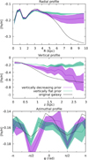 |
Fig. A.1. Profiles of [Fe/H] for the mock test for an inclination of 45°. From top to bottom: radial profiles (as a function of the cylindrical radius), vertical profiles, and azimuthal profiles. The green lines depict effects of the modelling assuming a flat vertical prior. The violet lines correspond to the optimal, vertically decreasing prior. Coloured bands show the respective uncertainties. The black lines shows the profiles of the target galaxy. We note that the data constrains extend only to R < 6 kpc. |
Appendix B: Impact of the radial prior
In our fiducial modelling approach, the initialisation of the population label depends only on the vertical coordinate. We could imagine imposing also a radial dependence. To test this possibility, we performed the same mock test as in Sect. 3.2, but imposing instead the following initial profile for the metallicity [Fe/H]i of each particle:
where G and N denote the gradient and its normalisation. Ri is the cylindrical radius coordinate of the ith particle and R0 is a normalisation constant, chosen as 1.3 kpc (to reduce correlation between G and N). The values that result in the lowest χ2 are G = 0.005 ± 0.012 dex kpc−1 and N = −0.24 ± 0.05 dex. The preferred range of the radial gradient is tightly constrained to the null value. In Fig. B.1, we present the impact of the radial initialisation on the final radial profile. The difference is rather small, well within the uncertainties of Fig. 3. We also inspected the impact of the radial prior on the shape of the azimuthal profile and it turned out to be minimal. Thus, our approach of using the initialisation that depends only on the vertical coordinate is justified.
 |
Fig. B.1. Initial (dashed lines) and final (solid lines) radial metallicity profiles of the mock galaxy. The green line marks the model with the lowest final χ2, while the blue and violet lines correspond to the 1σ-worse models. The black line shows the radial profile of the original mock galaxy. |
Appendix C: Asymmetry of the metallicity distribution
There are many asymmetries in the products derived from the data collected by Opitsch et al. (2018). The maps of the velocity dispersion and the fourth Gauss-Hermit moment h4 display asymmetry between the northern (Ry > 0, closer to us) and the southern (Ry < 0, farther away from us) part. Blaña Díaz et al. (2018) ascribed the asymmetries to the dust in the disc obscuring the central part of M 31. To correct that effect, they used the Draine et al. (2014) map of the dust in M 31. Assuming that the dust is concentrated in the disc plane, they employed the Draine & Li (2007) model to calculate the extinction along the line of sight. The resulting map of the fraction of the galaxy’s light that reaches us is shown in the middle panel of Fig. 22 in Blaña Díaz et al. (2018). The key feature of this dust model is that the light of the stars behind the disc plane is absorbed and contributes less to the observed properties than the stars in front of the disc plane.
In addition, the stellar populations maps of Saglia et al. (2018) display north-south asymmetries, most notably Hβ, age and metallicity (but not α-enhancement). In order to test whether the dust has an impact on the observed asymmetry of the metallicity distribution, we performed the following analysis. For each Voronoi cell, we computed the fraction of the light blocked by the dust, using the prescription outlined in the previous paragraph. We also calculated the [Z/H] asymmetry of each cell, that is, for a cell located at (Rx, Ry), we identified all the pixels located at ( − Rx, − Ry). The asymmetry comprises the difference between the cell’s metallicity and its reflection. It is positive if the reflection has a lower metallicity than the cell in question and negative otherwise. In Fig. C.1, we compare the dust-related transparency and the asymmetry of the data. We averaged the asymmetry of the Voronoi cells in the bins of the transparency. Besides simple arithmetic averages, we show averages weighted by the cells’ size on the sky, which accounts for significantly larger cell sizes far away from the M 31 centre. It is apparent that at low transparency the data has positive asymmetry (i.e. higher [Z/H] than on the other side).
 |
Fig. C.1. Mean metallicity asymmetry as a function of the light transparency through the dust. The green points were obtained weighting each Voronoi cell by its size on the sky, while the violet points show simple arithmetic averages. Error bars correspond to standard errors of the mean (corrected for the effective sample size for the weighted means). |
Given that the dust is a possible source of the asymmetry, we attempted two ways of mitigating the dust impact. In the first approach, we assumed that the whole northern side is compromised. We discarded that part of the data (i.e. the cells above the red line in Fig. 6), while the southern part was duplicated by rotating it by 180°, effectively making the data point-symmetric. Then, we proceeded to a fitting of an M2M model. The resulting face-on map is presented in the top panel of Fig. C.2. As expected, the map is symmetric with respect to the y = 0 line. It displays the metallicity-enhanced ring and a [Z/H] decrease farther away from the centre.
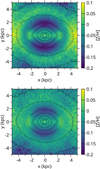 |
Fig. C.2. Face-on views of models fitted to two variants of the data. Top: southern part of M 31 (Ry < 0) point-symmetrised onto the northern part. Bottom: Voronoi cells fulfilling jointly two criteria (less than 80% of light throughput and metallicity asymmetry bigger than 0.1 dex) were discarded before fitting. |
In the second approach, we removed the Voronoi cells which jointly fulfilled two criteria: the non-attenuated light fraction was less than 80% (as derived using the discussed above dust model devised by Blaña Díaz et al. 2018) and the asymmetry was larger than 0.1 dex. The resulting face-on map of a model fitted to the filtered data is shown in the bottom panel of Fig. C.2. The metallicity-enhanced ring is still clearly visible in the bottom part of the map. The metallicity in the top part was reduced, however is was not enough to bring it into symmetry. In this approach, the asymmetry between the y > 0 and y < 0 parts was reduced from ∼0.2 dex to ∼0.1 dex.
As we mention in Sect. 4.1, the asymmetric feature persists for at least 6 Gyr when we let the model evolve freely. We decided to investigate which orbits are responsible for this phenomenon. To this effect, we evolved the model for 0.5 Gyr and every 10−4 Gyr, we recorded for each particle the position angle φ in the disc plane (in the reference frame rotating with the bar). Then, for each stellar orbit, we calculated the mean position angle ⟨φ⟩ and its standard deviation σφ. We show the distribution of the stellar orbits on the plane (⟨φ⟩,σφ) and their average metallicity in the top row of Fig. C.3. For an orbit that is symmetric with respect to the major axis of the bar, we expect ⟨φ⟩≈0°. If the orbit is axisymmetric, then their recorded φ are distributed uniformly, resulting in σφ ≈ 104°. These two numbers correspond to the highest peak in the orbital distribution. However, the distribution extends to much smaller values of σφ. In particular, there are two distinct populations of orbits with σφ ≲ 60°, located at ⟨φ⟩≈ ± 90°. The group of orbits clustered at ⟨φ⟩≈ + 90° has a higher metallicity than the group at −90°. We checked also the mean distance of those orbits and the result was ≈6 kpc, the same as the corotation radius. All these facts strongly suggest that the orbits around L4/L5 Lagrange points are responsible for a stable asymmetry. In the bottom row of Fig. C.3, we depict three such orbits.
 |
Fig. C.3. Source of the asymmetry of [Z/H] distribution. Top row: distribution of stellar orbits (left) and their mean metallicity (right) as a function of the mean position angle and its standard deviation. Bottom row: three examples of stellar orbits (in the rotating reference frame), revolving around the Lagrange points L4/L5. |
Given the existence of orbits supporting the asymmetry, it is possible that the asymmetry is, in fact, real. It could have arisen as a result of enhanced star formation in spiral arms on one side of the galaxy. In fact, the GALEX FUV image (Thilker et al. 2005) shows some asymmetry in the inner star-forming ring. However, if this were the case, we would also expect some asymmetry in the distribution of [α/Fe], which is not present.
To summarise, the apparent asymmetry of the M 31 metallicity data, and its model, can be related to the dust obscuration in its northern part. We hypothesise that the bulge stars are obscured by the star-forming disc, hence, the ages are biased towards the younger ones. This, through the well-known age-metallicity degeneracy, leads to an overestimated metallicity for the entire line-of-sight. The persistence of such an asymmetry in the model is supported by a presence of banana-shaped orbits related to the Lagrange points. On the other hand, since it is dynamically possible, it is conceivable that such a feature is actually a real one that is related to, for example, ongoing asymmetric star-formation activity. We note that some of the optically bluish galaxies presented in the appendix of Seidel et al. (2016) also show asymmetries in their Lick indices-based metallicity maps.
All Figures
 |
Fig. 1. Procedure for finding the correct initialisation of the vertical profile. Top panel: initial (dashed lines) and final (solid lines) vertical metallicity profiles of the mock galaxy. The green line marks the model with the lowest final χ2, while the blue and violet lines correspond to 1σ-worse models. The black line shows the vertical profile of the original mock galaxy. Bottom panel: map of final Δχ2 as a function of initial G and N in Eq. (5). Grey crosses indicate the actually computed models, while the underlying coloured map is a result of interpolation. Red contours depict 1-, 2-, and 3-σ regions. The red cross indicates the model with the lowest χ2. |
| In the text | |
 |
Fig. 2. Comparison of the model fit to the mock data. Top: mock map of mean [Fe/H] with a noise of σ[Fe/H] = 0.04 dex. Middle: best M2M dynamical model. Bottom: standardised residuals. The solid red line marks the position angle of the projected disc major axis, while the red arrows mark the orientation and the extent of the bar. |
| In the text | |
 |
Fig. 3. Metallicity profiles calculated from the model fitted to M 31-like mock data (violet, with a grey band of uncertainty), compared to profiles of the original model (green). The yellow lines show profiles resulting from a model fit to spatially-extended mock data. From top to bottom: radial profile (as a function of cylindrical radius), vertical profile, and azimuthal profile. |
| In the text | |
 |
Fig. 4. Metallicity maps of the Andromeda Galaxy. Top: map of the measured [Z/H]. Middle: best model. Bottom: standardised residuals. The solid red line marks the position angle of the projected disc major axis, while the red arrows mark the orientation and the extent of the bar. |
| In the text | |
 |
Fig. 5. Metallicity profiles calculated from the best model. From top to bottom: radial profile (as a function of the cylindrical radius), the vertical profile, and the azimuthal profile (black lines). The coloured bands show the different uncertainties. In red we mark the sum of the errors stemming from the uncertainties in the data and the vertical profiles, in blue we show the error range resulting from the uncertainty of the underlying dynamical model, and the green bands mark our final uncertainty estimates, which are the sum (in quadrature) of the three. We note that overlapping red, blue, and green appears as grey, and overlapping red and green as orange. Middle panel: the turquoise dashed line represents an uncertainty-weighted linear fit to the model curve. |
| In the text | |
 |
Fig. 6. Deprojected maps of mass-weighted mean [Z/H] in M 31. From left to right: face-on, edge-on and end-on view. Surface density contours are overplotted in the range of log(Σ/(M⊙ kpc−2)) = 8 − 10, with a multiplicative step of 101/3. |
| In the text | |
 |
Fig. 7. Metallicity profiles in three adjacent horizontal strips in the central region of M 31. The B/P bulge extends to x ≈ 2.5 − 3 kpc and z ≈ 1 kpc, while the bar length is ∼4 kpc. The maximum along the second (green) [Fe/H] profile corresponds approximately to the end of the B/P bulge. |
| In the text | |
 |
Fig. 8. Metallicity distribution of the bar-following orbits (top row) and the non-bar-following orbits (bottom row) in the face-on view (left column) and in the meridional plane (right column). The surface density contours are overplotted in the ranges of log(Σ/(M⊙ kpc−2)) = 7 − 9.5 (top row) and 8 − 10 (bottom row), in both cases with a log-step of 0.5. |
| In the text | |
 |
Fig. 9. Map of [α/Fe] enhancement in the Andromeda Galaxy. Top: measured [α/Fe]. Middle: best model. Bottom: standardised residuals. The solid red line marks the position angle of the projected disc major axis, while the red arrows mark the orientation and the extent of the bar. |
| In the text | |
 |
Fig. 10. Profiles of the α-enhancement, calculated from the fitted model. From top to bottom: radial profile (as a function of the cylindrical radius), vertical profile, and the azimuthal profile. Coloured bands show the different uncertainties as in Fig. 5. Middle panel: the turquoise dashed line represents an uncertainty-weighted linear fit to the model curve. |
| In the text | |
 |
Fig. 11. Deprojected maps of the mass-weighted mean [α/Fe] in M 31. From left to right: face-on, edge-on and end-on view. The surface density contours are overplotted in the range log(Σ/(M⊙ kpc−2)) = 8 − 10 with a multiplicative step of 101/3. |
| In the text | |
 |
Fig. 12. Distribution of [α/Fe] enhancement of the bar-following orbits (top row) and the non-bar-following orbits (bottom row) in the face-on view (left column) and in the meridional plane (right column). The surface density contours are overplotted in the ranges of log(Σ/(M⊙ kpc−2)) = 7 − 9.5 (top row) and 8 − 10 (bottom row), in both cases with a log-step of 0.5. |
| In the text | |
 |
Fig. A.1. Profiles of [Fe/H] for the mock test for an inclination of 45°. From top to bottom: radial profiles (as a function of the cylindrical radius), vertical profiles, and azimuthal profiles. The green lines depict effects of the modelling assuming a flat vertical prior. The violet lines correspond to the optimal, vertically decreasing prior. Coloured bands show the respective uncertainties. The black lines shows the profiles of the target galaxy. We note that the data constrains extend only to R < 6 kpc. |
| In the text | |
 |
Fig. B.1. Initial (dashed lines) and final (solid lines) radial metallicity profiles of the mock galaxy. The green line marks the model with the lowest final χ2, while the blue and violet lines correspond to the 1σ-worse models. The black line shows the radial profile of the original mock galaxy. |
| In the text | |
 |
Fig. C.1. Mean metallicity asymmetry as a function of the light transparency through the dust. The green points were obtained weighting each Voronoi cell by its size on the sky, while the violet points show simple arithmetic averages. Error bars correspond to standard errors of the mean (corrected for the effective sample size for the weighted means). |
| In the text | |
 |
Fig. C.2. Face-on views of models fitted to two variants of the data. Top: southern part of M 31 (Ry < 0) point-symmetrised onto the northern part. Bottom: Voronoi cells fulfilling jointly two criteria (less than 80% of light throughput and metallicity asymmetry bigger than 0.1 dex) were discarded before fitting. |
| In the text | |
 |
Fig. C.3. Source of the asymmetry of [Z/H] distribution. Top row: distribution of stellar orbits (left) and their mean metallicity (right) as a function of the mean position angle and its standard deviation. Bottom row: three examples of stellar orbits (in the rotating reference frame), revolving around the Lagrange points L4/L5. |
| In the text | |
Current usage metrics show cumulative count of Article Views (full-text article views including HTML views, PDF and ePub downloads, according to the available data) and Abstracts Views on Vision4Press platform.
Data correspond to usage on the plateform after 2015. The current usage metrics is available 48-96 hours after online publication and is updated daily on week days.
Initial download of the metrics may take a while.


![$$ \begin{aligned} {\mathrm{[Fe/H]}_i}(R_i) = G(R_i-R_0)+N, \end{aligned} $$](/articles/aa/full_html/2021/03/aa38381-20/aa38381-20-eq15.gif)