| Issue |
A&A
Volume 647, March 2021
|
|
|---|---|---|
| Article Number | A14 | |
| Number of page(s) | 23 | |
| Section | Numerical methods and codes | |
| DOI | https://doi.org/10.1051/0004-6361/202038123 | |
| Published online | 26 February 2021 | |
S2D2: Small-scale Significant substructure DBSCAN Detection
I. NESTs detection in 2D star-forming regions
1
Univ. Grenoble Alpes, CNRS, IPAG, 38000 Grenoble, France
e-mail: This email address is being protected from spambots. You need JavaScript enabled to view it.
2
University of Exeter, Stocker Road, Exeter EX4 4PY, UK
3
School of Physics and Astronomy, Cardiff University, The Parade CF24 3AA, UK
4
School of Physics and Astronomy, University of Leeds, Leeds LS2 9JT, UK
5
Quasar Science Resources, S.L. Camino de las Ceudas 2, 28232 Las Rozas de Madrid, Madrid, Spain
6
Leiden Observatory, Niels Bohrweg 2, 2333 CA Leiden, The Netherlands
7
Universidade de Vigo, Campus Universitario Lagoas-Marcosende, 36210 Vigo, Spain
Received:
8
April
2020
Accepted:
17
December
2020
Abstract
Context. The spatial and dynamical structure of star-forming regions can offer insights into stellar formation patterns. The amount of data from current and upcoming surveys calls for robust and objective procedures for detecting structures in order to statistically analyse the various regions and compare them.
Aims. We aim to provide the community with a tool capable of detecting, above random expectations, the small-scale significant structure in star-forming regions that could serve as an imprint of the stellar formation process. The tool makes use of the one-point correlation function to determine an appropriate length scale for ϵ and uses nearest-neighbour statistics to determine a minimum number of points Nmin for the DBSCAN algorithm in the neighbourhood of ϵ.
Methods. We implemented the procedure and applied it to synthetic star-forming regions of different nature and characteristics to obtain its applicability range. We also applied the method to observed star-forming regions to demonstrate its performance in realistic circumstances and to analyse its results.
Results. The procedure successfully detects significant small-scale substructures in heterogeneous regions, fulfilling the goals it was designed for and providing very reliable structures. The analysis of regions close to complete spatial randomness (Q ∈ [0.7, 0.87]) shows that even when some structure is present and recovered, it is hardly distinguishable from spurious detection in homogeneous regions due to projection effects. Thus, any interpretation should be done with care. For concentrated regions, we detect a main structure surrounded by smaller ones, corresponding to the core plus some Poisson fluctuations around it. We argue that these structures do not correspond to the small compact regions we are looking for. In some realistic cases, a more complete hierarchical, multi-scale analysis would be needed to capture the complexity of the region.
Conclusions. We carried out implementations of our procedure and devised a catalogue of the Nested Elementary STructures (NESTs) detected as a result in four star-forming regions (Taurus, IC 348, Upper Scorpius, and Carina). This catalogue is being made publicly available to the community. Implementations of the 3D versionsof the procedure, as well as up to 6D versions, including proper movements, are in progress and will be provided in a future work.
Key words: methods: data analysis / methods: statistical / Galaxy: structure / galaxies: star formation
© M. González et al. 2021
 Open Access article, published by EDP Sciences, under the terms of the Creative Commons Attribution License (https://creativecommons.org/licenses/by/4.0), which permits unrestricted use, distribution, and reproduction in any medium, provided the original work is properly cited.
1. Introduction
While a number of related processes have already been well established, a coherent and detailed portrait of stellar formation is not yet complete. Dynamical, thermal, magnetic, and gravitational effects may appear at all scales, producing an exceedingly complex and chaotic process (see e.g., Larson 2007, for a review). In particular, the specific relations between the geometry of parent clouds, prestellar cores, and young stellar objects (YSOs) are currently subject of very active research. Our current understanding is based on molecular clouds with intricate structures that undergo very complex fragmentation and where dense filamentary structures appear. These filaments, and particularly their intersections, host dense molecular cores and facilitate star formation (see Robitaille et al. 2019; Hacar et al. 2017, and references therein).
In such scenarios, star formation is not expected to occur in isolation, underlining the importance of taking into consideration the environmental effects that influence the whole process. The different effects that forming and young stellar objects can have on their environment (particularly if massive) suggests that the clustered environment of forming stars will have significant effects on a variety of observable phenomena, such as: high-mass star formation, protoplanetary disk survival, binary ratio, or the Hα cut-off observed in disc galaxies (see e.g., Pfalzner et al. 2012; Larson 2007; Reiter & Parker 2019; Pflamm-Altenburg & Kroupa 2008). The European project known as the StarFormMapper1 was initiated to study the influence of the natal environment on star formation.
Star-forming regions, henceforth SFRs, are the perfect observational laboratory for evaluating stellar-formation and evolution theories. In addition, large surveys such as Gaia and Herschel (Gaia Collaboration 2016; Pilbratt 2010) provide the scientific community with unprecedented quality and volume of data both on the gas and stellar components. These observations, coupled with simulations and the development of appropriate analytical and statistical techniques, will allow us to characterise the process leading from gas and molecular clouds to stellar clusters. In order to take full advantage of the data, the development of statistical methods, amongst other efforts, is required (Siemiginowska et al. 2019). In particular, we are interested in the development of robust, statistical procedures for the objective detection of significant spatial and spatio-kinematical structure. We ought to be able to ensure that the structures detected have the same observational properties, if not the same physical origin, to allow comparison amongst SFRs. The method must also be readily applicable in different regions while also guaranteeing the reliability of the structure detections.
We are particularly interested in small spatial structures in young, pristine SFRs, as in the research by Joncour et al. (2017, 2018; henceforth J17 and J18), which lays the theoretical foundation of this work. J17 and J18 are the only studies, to our knowledge, that focus specifically on the small, local scale and that compare the samples to a complete random distribution to ensure the significance of the structure retrieved. Traditionally, non-parametric clustering methods tend to discard clusters with low number of members due to the difficulty of distinguishing them from random fluctuations (see e.g. Kirk & Myers 2011; Gutermuth et al. 2009), while parametric methods choose such parameters as the number of clusters based on criteria associated to the likelihood of the underlying model (see e.g. Kuhn et al. 2014; Feigelson & Babu 2012). Through a meticulous analysis of the small-scale structure obtained in Taurus, J17 and J18 showed that these compact, local structures can be the imprints of the fragmentation of massive dense cores or clustering of cores.
The primordial nature and evolution of spatio-kinematical structure in SFRs, clusters, and associations are still active areas of inquiry. The complexity involved in the dynamical evolution of such systems is huge, represented by highly non-linear models strongly dependent on the specific initial conditions (see e.g., Aarseth et al. 2008; Clarke 2010). Spatial analyses of observations and simulations have been applied to density and radius estimation, membership, and multiplicity determination, as well as mass segregation (see e.g., Casertano & Hut 1985; Gomez et al. 1993; Larson 1995; Maíz-Apellániz et al. 2004; Cartwright & Whitworth 2004; Allison et al. 2009; Parker & Goodwin 2015; Maschberger & Clarke 2011; Buckner et al. 2019). In recent years, analyses have been extended to the spatio-kinematical phase space, allowing us to estimate the kinematical state of clusters and associations, generate catalogues, or distinguish between different populations within the Milky Way (see e.g., Fűrész et al. 2006; Parker et al. 2014; Wright et al. 2014; Alfaro & González 2016; González & Alfaro 2017; Parker & Wright 2018; Cantat-Gaudin et al. 2018).
Studies on the correlation of the degree of structure with age in open clusters (Sánchez & Alfaro 2009; Dib et al. 2018) indicate that if such a correlation exists, it is weak. Simulations from Parker & Meyer (2012) point to a rapid erasure of primordial structure, which is in agreement with Fujii & Portegies-Zwart (2016), who propose that clumpy SFRs lose their structure through the expulsion of residual gas and two-body relaxation.
However, Hetem & Gregorio-Hetem (2019) also analysed a large sample of clusters, finding that according to their mass segregation indicators, ΛMSR and ΣMST (as introduced in Allison et al. 2009; Maschberger & Clarke 2011) their structural characteristics did not change within their first 10 Myr of age, although it must be noted that clusters in their sample have a relatively low degree of structure. Pfalzner et al. (2012) performed simulations of single and multimodal clusters (formed by two or more single clusters combined in one sample) and evaluated local surface and nearest-neighbour methods to find the theoretical density profile and modes. They found that incompleteness and resolution can prevent the distinguishing of modes and that cluster age is not a reliable indicator of dynamical state, at least for embedded clusters. In addition, they about urge caution when considering the reliability of age estimates in the context of several low-mass clusters into a single sample. These subsamples are typically not at the same evolutionary stage and some of them may still be forming stars. Including these very young subclusters in the average calculation is meant to keep the global age estimates low for a variety of clusters with different ages for the older subsamples.
Considering all this, there are still significant chances that the structure in young, clumpy SFRs is primordial and reflects the nature of the star-forming process in a particular region. In that case, analysing the reliable, significant small-scale structure will help better understand the characteristics of the process. Even if the structure were not primordial, the objective method of structure retrieval presented in this work makes them relevant and robust, allowing for a statistical comparison of the characteristics of different SFRs.
In this work, we analyse the behaviour and define the range of applicability with regard to S2D2, which is a procedure based on the method in J17 and J18 and which was successfully applied in Taurus to retrieve significant small-scale structure. To that end, as described in Sect. 2, we have developed an automatic tool, S2D2, and tested it in simulated SFRs of various natures. We have also applied the procedure to four observed SFRs (Taurus, IC 348, Upper Scorpius and Carina), evaluating its performance in realistic situations. In Sect. 3, we show the results of the procedure on synthetic SFRs that will allow us to define the range of applicability of S2D2. Section 4 shows the results of further testing of the procedure on observed SFRs. Finally, in Sect. 5 we will summarise the main results and conclusions from this work. We note that even though in this paper we will treat only two dimensions, the procedure can be readily extended to 3D and up to 3+3D, and these versions will be also made available for the community. Appendix A presents information on the different implementations of the procedure that are publicly available.
2. Description of S2D2
The S2D2 procedure combines a classic data mining algorithm as DBSCAN with a statistically sound, theoretically rooted method to choose its parameters so that it searches for the smallest scale significant structures in a sample. Its basis was developed and extensively discussed in J17 and J18, where it was successfully applied to Taurus, a characteristic example of a very young and structured SFR. In that work, the small-scale significant structures (which we also refer to as Nested Elementary Structures, or NESTs, following their nomenclature) had a high likelihood of serving as the pristine imprints of the stellar formation process. In the following, we briefly explain the procedure and the slight modifications and additions that allow its robust application in a general case.
2.1. DBSCAN
We now present the commonly used clustering algorithm known as Density Based Spatial Clustering of Applications with Noise (DBSCAN, introduced in Ester et al. 1996), which is a general-purpose data-mining algorithm that has been widely used in a variety of contexts, including structure detection in spatio-kinematical domains (see e.g., Costado et al. 2017; Cánovas et al. 2019; Kounkel & Covey 2019, and references therein). We refer the reader to the appendix in J17 or the report by Joncour et al. (2020) for an in-depth review of DBSCAN and other clustering methods.
As its name indicates, DBSCAN detects clusters or structures in a specific domain according to density criteria, introducing an associated concept of reachability that characterises all the points in a cluster. This density requirement is based on two parameters: a length scale, ϵ, and a minimum number of points, Nmin. A point, p, in a point pattern is a core point if there are at least Nmin − 1 different points of the pattern within a distance, ϵ, of such point (also called the ϵ-neighbourhood or vicinity). All the points in an ϵ-neighbourhood of a core point are said to be directly (ϵ-)reachable from that core point and are assigned to the same cluster. The reachable points that fulfill the Nmin condition are also core points of the cluster, while those reachable points that do not satisfy the condition become border points. The points that are not directly reachable from a core point and do not meet the Nmin requirement are labeled as noise.
Figure 1 shows four stages of the application of DBSCAN algorithm to a sample, illustrating several possibilities that will be mentioned in this section. The first panel shows the detection of the first core point, p, defining cluster C1. In the second panel, more points of C1 are detected alongside the study of the environment of the already-known members of C1. Panel 3 shows a second identified cluster, C2, and panel 4 shows the final stage of the algorithm, where a third cluster, C3, has also been identified.
 |
Fig. 1. Application of DBSCAN algorithm to an example sample. Each panel represents one step in the process, with panel 4 showing the final result of the algorithm. The grey dots represent points that are not assigned to any cluster (noise points in panel 4), while the coloured, big dots depict points assigned to clusters (C1, C2, and C3) and each cluster is represented with a different colour. Coloured points with a black border are core points in a cluster, while those without one represent border points. Black circles show the ϵ environment of some representative points, which are also labeled. First panel: depicts the detection of a cluster within the sample. The ϵ-vicinity of the point labeled as p has more than Nmin = 5 sample members within, so p is identified as a core point (represented as a black-edged, coloured point) of the first identified cluster, C1, and the points within its ϵ-neighbourhood are marked as blue, since they are directly reachable from p and, thus, belong to the cluster C1. A subsequent step is to check the ϵ-vicinities of these points belonging to C1, which leads to the discovery of new members of C1, and the classification of some of them as core points. Bottom left panel: a latter epoch in the algorithm application, where a second cluster C2 composed only of core points is identified. Last panel: final results of the algorithm, where a third cluster, C3, with a single core point, is identified. The point q is in the ϵ-vicinities of core points in C1 and C3, so it will be assigned to either cluster depending on the processing order of the points. |
The parameters ϵ and Nmin define a minimum local density requirement for core points, that we will call nominal density  . This density ρnom is not necessarily the minimum local density of the clusters, since, by definition, the border points belonging to a cluster do not have to reach it. This means that the DBSCAN algorithm is not completely equivalent to a cut in local density since the minimum local density of the members of a cluster will be that of its border points. Also, the parameter Nmin is not necessarily either the minimum number of points in each cluster. Even though DBSCAN is a hard clustering method (meaning that each point will belong to only one cluster, if any), in some situations, border points can be assigned to different clusters depending on the order of processing by the algorithm. This is illustrated in Fig. 1, where the point labeled as q does not reach the minimum number of points in its ϵ-vicinity, but it belongs to the ϵ-vicinity of a core point in C1 and also a core point in C3. The point q is assigned to cluster C1 because it was identified first, but it is located on the boundary of both C1 and C3, so if the core point of C3 had been processed before p, q would be assigned to C3. As a result of this configuration and the point processing order, C3 has only 4 = Nmin − 1 members.
DBSCAN is one of the few classic algorithms where noise is handled, meaning that not all the points in the sample are assigned to a cluster. This is a necessity when dealing with such problems as the one at hand, where it is only the relevant substructures that must be retrieved. Another advantage of the algorithm is that it can detect clusters of arbitrary shape and does not impose any a priori number of substructures in the sample. The main drawback of the algorithm is the single-scale ϵ used to search for structures, which may not realistically reflect the complex nature of all SFRs. To overcome this issue, a multi-scale, hierarchical extension of this method, following the philosophy of choosing relevant length scales and number of points guaranteeing reliable structures, is in development and has been presented in Joncour (2019).
2.2. Selection of the size scale ϵ: one point correlation function
In this section, we will use some definitions from the spatial statistics field, which studies the statistical distribution of objects within a spatial domain (point patterns). In this work, we will focus on point distributions given by the positions of stellar objects in SFRs, but more general domains can be considered. The most basic point distribution is complete spatial randomness, where the probability of having n objects within a specific region is only dependent on the volume of the region. We refer to complete spatial randomness by its acronym (CSR) or as homogeneous distributions. The CSR distributions are described by a Poisson distribution with constant density (or intensity) and represent distributions of points without mutual interaction. In spatial statistics, CSR serves as reference to compare the characteristics of more complex and real-life derived distributions, where interactions and other phenomena are expected to occur. We refer the reader to Diggle (2003), Illian et al. (2008) for a comprehensive introduction to spatial statistics and point patterns; and to Feigelson & Babu (2012) for its astronomy applications.
There are several tools that are useful when comparing a specific point distribution to the CSR and evaluating whether it is compatible with CSR, clustered, or inhibited. Throughout this text, clustering (resp. inhibition) means that the points are closer (resp. more separated) than the random expectation. The pair correlation function g(r) (PCF) compares the distribution of distances in the sample with that of a random distribution, and is described by the ratio of the observed distribution and CSR, as a function of distance r. Distances where g(r) > 1 indicate an excess of pairs with distance r compared to random and, conversely g(r) < 1 indicates a deficit. The slopes of g at small scales have been used to distinguish stellar binaries, clusters, and associations (e.g., Gomez et al. 1993; Larson 1995; Kraus & Hillenbrand 2008). The PCF (or equivalent functions such as the two point correlation function) has been used traditionally in astronomy to quantify the spatial distribution of galaxies (Peebles 1980) and is indicated by Retter et al. (2019) for the testing of CSR in the context of SFRs. It is, however, not exempt of problems, such as its dependence on the geometry and size of the window where the spatial distribution is defined. The PCF measures second order statistics, variance and covariance, associated to interactions between points such as attraction or repulsion.
J17 introduced the one point correlation function (OPCF), Ψ(r), which is given by the ratio of the distribution of the first nearest neighbour in the sample and that of a homogeneous distribution. As the ratio of the sample and CSR distributions at different scales, the OPCF resembles the PCF, but it measures first-order effects associated to density variations in the study area and it is also less sensitive to edge and size effects from the window, particularly at short scales (as shown in J17). The choice of the first nearest neighbour ensures that we are considering the closest environment of each star, treating the smallest possible scales. Analogously to the pair correlation function, distances, r, where Ψ(r) > 1 indicate an excess of stars with nearest neighbour at distance. r, compared to random and, conversely, Ψ(r) < 1 indicates a deficit.
The size scale ϵ for DBSCAN is chosen by S2D2 following J17 and J18, as the smallest transition distance between excess and deficit of stars with respect to CSR in terms of the OPCF, where Ψ(ϵ) = 1. Given the OPCF definition, stars whose nearest neighbour is at a distance smaller than ϵ are clustered, compared to the theoretical expectation for CSR.
As functions based on local properties, both the one point and the pair correlation functions are evaluated at different scales, r, within the sample. In practice, this is usually done with histograms that discretise the range of densities involved (e.g., Larson 1995; J17; J18; Kraus & Hillenbrand 2008). Histograms pose an issue, namely that the size (or number) of bins needs to be carefully chosen depending on the sample to avoid empty bins and also reflect variations. In this work, we avoid this issue by using a Gaussian kernel representation for the first nearest neighbour density where the bandwidth h is computed using Silverman’s formula (Silverman 1986), which is given by:
 (1)
(1)
where n is the size,  the standard deviation, and IQR the inter-quartile range of the sample. We performed additional tests with the more complex Botev’s algorithm (Botev et al. 2010) to calculate the bandwidth, but it did not improve the results. In fact, the ϵ estimates obtained from the OPCF calculated using both bandwidths are very close, as shown in Appendix C. As a consequence, we keep using Silverman’s formula, which is simpler and much more popular. We note that the OPCF values are dependent on the density of the region, which is used to derive the first nearest neighbour distribution for CSR, which in turn is associated to the window chosen for the study. In order to obtain a robust procedure that can be applied without the need to explicitly study each region to choose an appropriate window, we rely on nearest-neighbour statistics. The probability density function of the kth nearest neighbour in a 2D CSR distribution is given by J17:
 (2)
(2)
where ρCSR is the density or intensity of the CSR point distribution, and Γ represents the Γ (gamma) function2. The expected value of the kth nearest neighbour distance is then:
 (3)
(3)
If we solve Eq. (3) for the intensity of the process ρCSR, we obtain:
 (4)
(4)
where we have substituted for k = 6, an intermediate value which balances the locality of the estimate and the smoothing of random fluctuations for a variety of sample sizes according to Casertano & Hut (1985). They argue that lower values of j (such as j = 3) are well-suited for regions with a very small number of particles, Nstar < 30, but in the case of larger simulations could include noise, biasing the estimates. Later work using local density estimates (such as, e.g., Parker & Goodwin 2015; Maschberger & Clarke 2011; González & Alfaro 2017; Buckner et al. 2019, amongst others) has confirmed that values for j between 5 and 7 are appropriate for 2D and 3D distributions. The expression we propose for the density of the region, ρCSR in Eq. (4) is formally equal to the unbiased estimator for the local density proposed by Casertano & Hut (1985) based on the 6th nearest neighbour Σ6, differing from it only through a constant factor of ∼1.15. Our choice of a representative density for the region to make a fair comparison with CSR (ρCSR) is thus coherent with our method and with classical estimators of local density.
2.3. Selection of the minimum number of points Nmin and the significance of the retrieved substructure
As in all statistical distributions, CSR patterns show noise and deviations from their theoretical distributions due to finite sampling effects. This implies that when generating a point pattern with constant, uniform density the points are not evenly distributed within the volume. Such fluctuations in local density for CSR can be detected and interpreted as significant structure instead of noise.
The nearest-neighbour distribution can help us evaluate the theoretical probability of finding fluctuations with a particular density, as developed in J18. For a CSR distribution, the probability α of having k companions within radius r is given by the integral between 0 and r of the kth nearest neighbour probability density function, as shown in Eq. (2). This value α is the statistical significance level of a structure of k + 1 members in a r neighbourhood and 1 − α is its confidence level. If we fix r and ρCSR, the confidence value of a structure with respect to random fluctuations increases as we increase the number of neighbours k requirement. It is also interesting to note that for fixed r and k, the confidence value decreases as we increase the density of the region.
Taking all this into account, we require a confidence level larger than 3σ, namely, (1 − α) = 0.9985, to consider the structures significant, using the scale ϵ and the density ρCSR chosen by our procedure as previously described. In other words, we chose Nmin = k0.0015 + 1, with k0.0015 being the smallest number of neighbours k for which the confidence level of the structures found is above 0.9985.
The Nmin obtained and the strict level of confidence imposed by S2D2 implies that we may be losing some real, significant structure that is not statistically distinguishable from random fluctuations in a clear way. We made a conservative choice between completeness and reliability of the detections for the sake of obtaining structures that can be interpreted and compared across different clusters.
2.4. Summary of the algorithm
Here, we summarise the three main steps involved in running the S2D2.
The first step is choosing the relevant ϵ scale of the substructure that we search for, as explained in Sect. 2.2. This involves calculating a representative density of the region to be used for comparison with a random distribution ρCSR. Next, the first nearest-neighbour distribution and the OPCF are computed. Finally the transition scale ϵ from excess to deficit of stars with respect to CSR is obtained.
The second step is to choose the minimum number of points Nmin to guarantee the significance of the retrieved substructure (Sect. 2.3). For the ϵ value previously obtained, we iteratively increase the Nmin until a fixed significance value of 1 − α is reached.
The third and last step is to apply DBSCAN with the obtained ϵ and Nmin and retrieve the NESTs in the region.
3. Results
3.1. Tests of S2D2 in synthetic clusters
We start the analysis of the behaviour of the procedure using simulated test clusters (which represent the stellar content of SFRs), where the underlying distribution is, by construction, known.
The test clusters display a variety of characteristics, allowing us to determine the range of applicability of the method. This way, we can ensure that the structure found is significant and that the comparison and analysis of structure across different regions is coherent and robust.
3.1.1. Synthetic cluster generation and treatment
For each of the distributions in Table 1, we simulated 10 3D clusters (i.e. ten different realisations of each distribution) with Nstar = 1000 points each. The number of bona fide members of observed clusters is between is typically between 100 and 10 000 (see e.g., the survey by Cantat-Gaudin et al. 2018) so studies with synthetic clusters also use those ranges for Nstar (see e.g., Jaffa et al. 2017; Lomax et al. 2018; Parker 2018). Even though we do not specifically explore the effect of Nstar in our procedure here, larger (resp. smaller) values of Nstar will sample better (resp. worse) the theoretical underlying distributions, making it easier (resp. harder) to distinguish them. In Fig. 2, we show an example realisation of each of the distributions in Table 1.
Spatial distributions, with parameters and references used to generate synthetic clusters.
Fractal distributions of all dimensions were generated with McLuster (Küpper et al. 2011) without imposing any radial gradient and the radial ones were generated according to the recipe in Cartwright & Whitworth (2004; henceforth CW04). These distributions produce regions with varying levels of substructure and concentration. We also included a Plummer distribution, using the generating function in Aarseth et al. (2008), to account for concentrations of different nature. The regions sampled from fractal distributions range from highly structured (fractal dimension D = 1.6) up to homogeneous regions (fractal dimension D = 3.0). Similarly, radial distributions show different levels of concentration, according to the exponent of their density. They range from homogeneous (exponent E = 0) to highly concentrated regions (exponent E = 2.5). We note that in the case of concentrated regions, by construction, the density has a gradient, which is larger when the concentration exponent is larger. The fractal distribution with dimension with D = 3.0 and the radial distribution with E = 0 produce homogeneous distributions that are statistically equal to CSR since they are different ways to generate the same theoretical Poisson homogeneous point distribution with constant density.
As for the Plummer models, the specific scale radius, rPlum, defining the core size is not important in itself, since, as we explain later, the clusters are rescaled afterwards. However, in practice, the generating function is not bounded in terms of radius, so a cutoff radius is usually enforced to avoid the appearance of very extreme outliers. We have chosen  since the theoretical Plummer model has ∼95% of its mass within 5 rPlum.
In all cases, for the sake of easing the comparison amongst regions, simulations were translated and rescaled to the approximate position and size of the Taurus SFR (allowing comparison with J17 and J18), setting the units so the radius of the cluster is ∼9 deg at Taurus’ distance of 145 pc without modifying the relative sizes of the axes. Then the 3D clusters were projected into (RA,Dec) coordinates, to mimic the 2D data available in observations of young stellar objects in SFRs. Finally, the sample was treated for binaries and chance alignments in projection, merging multiple systems (considering as part of a multiple system objects at separations below 1000 AU) into one single object, as done in J17 and J18. The limit of 1000 AU was chosen in these works for two reasons: it is close to the resolution limit in the regions, and it also is within the lower separation estimates for wide binaries. After merging multiple systems in the initially generated sample of 1000 stars, the final number of objects in each synthetic star-forming region is between 966 and 1000.
3.1.2. Synthetic cluster description
For all synthetic star-forming regions, we have calculated the structure parameter Q introduced in CW04.  is the ratio between the normalised mean branch length of the minimum spanning tree
  , and the normalised mean distance between points
  . The scale-free Q structure parameter has been widely used to quantify the structure of stellar clusters, star-forming regions, and even dense cores (Alfaro & Román-Zúñiga 2018; Parker 2018) since fractals have low Q values, lower for lower fractal dimension, while radial distributions have large Q values, increasing with the concentration. There is even a threshold of Q = 0.8 that can separate concentrated from structured regions, corresponding to homogeneous distributions. The limit values D = 3 for fractal distributions and E = 0 for radials both correspond to a homogeneous distribution, with a constant density and the Q values obtained from approaching homogeneity from both perspectives converge.
Figure 3 shows the typical local density of a region ρCSR (used for comparison with random and calculated using Eq. (4)) against the Q parameter for all the simulations, with colours and shapes marking the type of distribution for each synthetic cluster. Both the strength and limitations of the Q parameter are clear from the plot: in effect, each distribution has a specific range of Q values, that can be associated to their substructure or concentration, and in addition, the Q values for the homogeneous distributions, approached both from a fractal and radial density, are coherent. The drawback of the Q parameter is that the dispersion amongst realisations of a single distribution, larger for fractals, causes an overlap that makes it difficult to distinguish between distributions, particularly when they are close to homogeneous. Despite its limitations, which are discussed in Appendix B, we used the Q structure parameter to graphically separate the synthetic distributions in the plots and as a global indicator of the presence of substructure, as recommended by Daffern-Powell & Parker (2020).
 |
Fig. 3. Density against the Q structure parameter for all synthetic regions. Different symbols indicate whether the parent distribution is fractal or radial, while colour indicates a different parent distribution. |
From Fig. 3 it is clear that the density of the region is associated to its level of structure, given that we have rescaled all the synthetic regions to guarantee that their sizes are comparable. The density of a region ρCSR increases with both substructure and concentration. This is an expected and desirable behaviour, since both structured and concentrated simulations are examples of clustered patterns, characterised precisely for their excess of stars at small distances, which decreases the average 6th nearest neighbour distance with respect to random. In other words, their average local density Σ6 is larger. Analogously to the Q parameter, the density of the region ρCSR is more disperse in the case of structured regions, and the density values of both the fractal and radial approximation to an homogeneous distribution are similar. The Plummer distribution, being outside the Box-Fractal/radial model paradigm, exhibits a behaviour that globally corresponds to a concentrated distribution (large Q and ρCSR values) but nevertheless different from the radials.
The top panel of Fig. 4 shows the parameter ϵ for each synthetic cluster calculated as described in Sect. 2.2 against the Q structure parameter, with the same symbol and colour code as in Fig. 3. The ϵ scale parameter is, in general, smaller for both more structured and more concentrated regions, and larger for homogeneous. This is consistent with the fact, shown in Fig. 3, that structured and concentrated clusters are also locally denser than homogeneous. In general, ϵ shows significant dispersion, particularly for clusters approaching homogeneity and obtained from radial distributions, where very small ϵ values can appear. This is expected from the method, since the OPCF is close to complete spatial randomness and the threshold ϵ such that Ψ(ϵ) = 1 (separating excess from defect of stars with nearest neighbour at distance ϵ) can be crossed by fluctuations at a variety of distances. For an illustration of the summarised behaviour of the OPCF for the different synthetic clusters in this work, we refer to Appendix C. We note that the method is devised for substructured regions, characterised by star distributions where some pristine substructure associated to the cloud fragmentation might be retained.
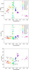 |
Fig. 4. Top: ϵ scale parameter for DBSCAN calculated with the procedure presented in Sect. 2.2 against Q structure parameter. Middle: relative nominal density of the detected structures ( |
To clarify the relationships between structure, scales, and densities, we have weighted the nominal density ρnom of the structures detected by DBSCAN (as described in Sect. 2.1) with the density of the regions ρCSR (henceforth, the relative nominal density of the structures, or ρnom/ρCSR) and plotted it against the Q structure parameter, as shown in the middle and bottom plots of Fig. 4. The middle plot is in logarithmic scale, to show the complete span of values reached, and the bottom plot is zoomed and in linear scales. This panel shows a clear trend of larger relative nominal density required for concentrated regions. A similar, slight increasing trend of relative nominal density with fractality is also present, but it is not as obvious as with concentration. This is partly due to the fact that regions close to CSR show very large dispersion, as was the case with ϵ in the previous panel. We note that the nominal density required for substructure detection is in all cases larger than 8.8 times the density of the region, confirming the strict criteria for significance in S2D2.
In addition to the results in synthetic clusters, Fig. 4 and all the following figures in this section also contain the values of the observed clusters analysed in Sect. 4. As will be shown in more detail in Sect. 4 and Appendix B, the simple Box-Fractal/radial and Plummer models do not capture all the features in real clusters, with the exception of IC 348.
Figure 5 shows the number of structures detected in each region against the Q parameter. Despite the dispersion, there is a clear trend coherent with the expectations and objectives from the method proposed. The more structured a region, the larger the amount of small-scale significant substructure detected, with homogeneous regions showing almost no traces of significant structures.
 |
Fig. 5. Number of structures detected with the procedure against Q structure parameter. Colours and symbols represent parent distributions, with the same colour and symbol code as in Fig. 3. |
It is important to mention that there are cases where some structure can still be detected by the procedure in homogeneous regions, due to the projection of 3D structures. The retrieval of this spurious structure in S2D2 is not frequent, but projection effects should not be confused with substructure to avoid the over-interpretation of results. We note that the Q values and thresholds used in this work correspond to the 2D analysis of 3D data and, thus, take into account projection effects. A cut in the Q parameter of 0.7 will discard some quasi-homogeneous structured regions, but gives more than a 2σ certainty that we are dealing with a structured region, considering CW04, Cartwright (2009), Sánchez & Alfaro (2009), and covering an ample range of sample sizes. Analogously, regions with Q between 0.8 and 0.87 are within the 2σ dispersion range of homogeneous regions and also contain regions of light concentration. In clusters with Q values within these ranges, special care must be taken to try and distinguish whether they are projected CSR.
It is also clear from Fig. 5, in general, that the number of structures detected also increases with concentration. This is an effect associated with the density distribution of these samples that, by construction, have a density gradient. In subsequent sections (specifically, in Sects. 3.4 and 4) we will explain this effect in more detail. The fact that real observed regions, shown as black stars in Fig. 5, show in general a larger amount of structures than simulations with a close Q parameter value will be discussed in Sect. 4, where we analyse the results of S2D2 applied to real data and the differences with simulations.
Figure 6 shows two additional results from the application of the procedure. The top plot in Fig. 6 shows the fraction of stars belonging to NESTs against the Q structure parameter. There is a clear trend for concentrated regions, where the fraction of stars within structures reaches almost 30% for radial distributions and 50% for Plummer. There is also a slight tendency of more fractal distributions to have a larger amount of stars belonging to NESTs. These trends are partly due to the larger amount of structures detected in concentrated and structured regions (as shown in Fig. 5), but also to the fact that the structures themselves are larger for concentrated regions. To explore this last effect, in the bottom plot of Fig. 6 we show the relative maximum population of NESTs, given by the ratio of the maximum number of stars of a structure Nmax and the minimum number of points required by the procedure Nmin. For highly concentrated regions, this ratio is larger than 10 meaning that at least one of the structures is too abundantly populated to be considered small scale. We cannot give an objective strict limit for large scale structures, but given the results for synthetic regions, Taurus, and Upper Scorpius in Fig. 6, it is reasonable to individually study all the characteristics of a region before deciding whether it is concentrated, particularly for values of  between 5 and 10.
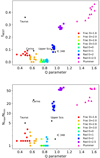 |
Fig. 6. Top: fraction of stars in NESTs against Q structure parameter. Bottom: relative maximum size of structure detected Nmax weighted by the significant number of points Nmin against Q structure parameter. Colours and symbols represent parent distributions, with the same code as in Fig. 3. |
Table 2 shows a summary of the general results of the simulations. The sample mean and standard deviation give us a central and dispersion measurement of the magnitudes calculated in this work across all the realisations of each distribution.
Sample mean ± sample standard deviation of the procedure results in synthetic clusters, grouped by distribution.
3.2. Fractal clusters
Figure 7 shows examples of synthetic structured clusters, where the complete sample is depicted by grey dots and the stars in the detected substructures are shown as coloured squares. The upper plot in Fig. 7 shows an example of a fractal cluster with fractal dimension D = 1.6, the smallest used in this work. The general sample is highly structured, with obvious clumps of stars of different size. The procedure detects several significant structures in the southern and central part of the sample, while the structures that can be identified by visual inspection in the northern areas are deemed not significant. The compactness and small scale of the structures found is evident. The middle panel of Fig. 7 shows the significant structure in a fractal synthetic cluster with dimension 2. The region is clearly structured, although the clumps present are less dense and clear than in the example of fractal dimension D = 1.6. Four small compact significant structures are detected by the procedure, marked in colour. The lower plot in Fig. 7 shows a synthetic fractal cluster with dimension 2.6. This distribution is relatively close to CSR, and the structured nature of the distribution is not clear at all. Our procedure only detects one structure, small and compact, fulfilling the requirements of significance.
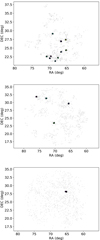 |
Fig. 7. Top: map of structures in a fractal with D = 1.6. Middle: same for a fractal with D = 2.0. Bottom: same for a fractal with D = 2.6. Noise stars are in grey, while stars in structures are shown as coloured squares. Each shade of purple, blue, green, and yellow represents a different small-scale structure retrieved by S2D2. |
We can assert that in structured regions, the structures found by S2D2 are small, compact, and very reliable. There is a trade-off between the reliability and retrievability of structures, where we have obviously favoured reliability, even at the risk of losing some of the structure. We believe that this is important in a systematic procedure for statistical comparisons amongst regions, minimising the chance of including artefacts in such comparisons. In the implementations available for the community, the user will be able to manually introduce a value of ϵ and Nmin for DBSCAN, relaxing the ρnom required for detection.
3.3. Homogeneous clusters
Figure 8 shows maps of synthetic regions drawn from both the fractal and radial recipes to obtain a CSR distribution, the fractal with dimension D = 3 and the radial with exponent E = 0. It is clear that the stars in these CSR samples are not evenly distributed in the spatial domain and show density variations. These are a combination of statistical fluctuations and projection effects.
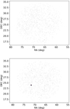 |
Fig. 8. Top: map of structures in a fractal with D = 3.0. Bottom: same for a radial with E = 0.0. Noise stars are in grey, while the purple squares in the lower plot belong to a significant structure retrieved by the procedure. |
The upper plot shows the fractal with D = 3, where S2D2 finds no significant structure, and the bottom panel shows a region with radial distribution, where despite the strict level of significance (in this particular case, the nominal density, ρnom, required for detection is more than a factor of 100 larger than the density of the region), some of this structure is retrieved by the procedure and shown in purple.
In any case, as previously explained, we are warned by the Q values associated to these regions (0.79 and 0.8, respectively) to carefully analyse and decide whether the structure retrieved could be significant or an artefact due to projection effects.
3.4. Concentrated clusters
Figure 9 shows examples of synthetic clusters drawn from concentrated distributions (radials with exponents E > 0 and Plummer). From top to bottom and left to right, the panels show radials with exponent 1, 2, and 2.5, and a Plummer distribution. In all four cases, the plot is restricted to the central part of the cluster. The increase of concentration with the exponent for radials is clear from Fig. 9, as is the different nature of the concentration in the Plummer case. The growing amount of structures detected with concentration that we mentioned in the previous section is clear and its pattern can now be seen: the central concentration characterising these clusters is retrieved as a large structure, surrounded by smaller secondary structures; generally, the larger the concentration, the larger the central structure and the larger amount of secondary structures. For the Plummer example several large structures can be distinguished next to each other in the central area. In the case of low central concentration (as with E = 1 in the top left panel of Fig. 9), the central structure is not significantly retrieved, and only some secondary structures are there. Despite being concentrated, examples of this distribution are close to CSR, as indicated by the Q values close to 0.84, so the central increase in density is not clear.
 |
Fig. 9. Maps with the structures found using the procedure, e.g., simulations drawn from concentrated distributions. From left to right and top to bottom: radial with exponent E = 1.0, radial with E = 2.0, radial with E = 2.5, and Plummer, respectively. Noise stars are represented as grey dots, while the stars belonging to substructures are squares coloured in different shades of blue, purple, green, and yellow according to the small scale structure that they belong to. We note that only the central area of the clusters is shown, so the retrieved substructure is clearer. |
The secondary structures are a consequence of the density gradients present in these samples, which are, by construction, proportional to their degree of concentration. A large density gradient implies that the range of densities present in the sample is also large, so the choice of a single density (no matter how carefully done) does not represent the complexity of the sample. Secondary structures represent Poisson fluctuations at densities larger than ρCSR, the region density.
Concentrated regions are beyond the scope for which S2D2 was originally designed since they do not present the kind of local small-scale structures that we search for. In addition, simulations carried out by Parker & Meyer (2012), Daffern-Powell & Parker (2020) to study the persistence of substructure indicate that it is quickly erased through dynamical interactions, with the Q parameter increasing rapidly. Thus, the concentrated regions could be dynamically evolved, devoid of spatio-kinematical traces of stellar formation. This is in agreement with Sills et al. (2018), where they used the extension of Q, Q+ to quantify the structure. We refer the reader to Appendix B for more information on these tools. The fact that even in these cases the behaviour of S2D2 is consistent, finding the large main structure with Poisson fluctuations around, is a sign of the robustness of our procedure. For cases such as this, a multi-scale approach of the structure analysis, as in Joncour (2019, and in prep.) would allow us to distinguish these fluctuations, capturing the complexity of the density pattern in the region.
4. Results for observed clusters
In this section, we show the results of a further testing of the procedure, this time in observed clusters, that will allow us to calibrate its limits in realistic samples, beyond the idealised nature of synthetic clusters. The catalogues of substructure found in these four regions can be accessed from the StarformMapper web.
Table 3 shows a summary of the results of applying S2D2 to four test cases: Taurus, IC 348, Upper Scorpius, and Carina, which constitute a varied sample of initial conditions. We have processed the YSO samples in all regions to merge multiple systems using the same distance limit of 1000 AU used in the simulations and in J17and J18 for Taurus despite the different distances at which they are located. This does not hinder the calibration objective we pursue in this section, but we recommend a careful consideration of the spatial resolution and method used to obtain the sample members of a cluster before studying its substructure with S2D2, or any other tool.
Results of the procedure in real clusters.
In the following, we describe the specific results in each region.
4.1. Taurus
We first test the proposed method in the Taurus region, which, as a young (1−2 Myr) and close (140 pc) SFR has been the object of numerous studies (see e.g., Kenyon et al. 2008; Luhman et al. 2010, and references therein). Taurus is a typical example of a structured region, making it perfect for checking the correct behaviour of the procedure. J17 and J18 found and studied in detail ultra-wide pairs and significant small scale structures of higher multiplicity, NESTs, proposing that they are pristine and reflect the characteristics of the cloud fragmentation process. These works set the basis of the method presented in Sect. 2. In this work, we use the updated catalogue from Luhman (2018), which has ∼100 more members than the sample by Luhman et al. (2010) used in J17 and J18. The sample in Luhman (2018) also includes data from Gaia DR2, a significant portion of which includes parallax and proper motion information, so this analysis will be extended into more dimensions in a future work.
The original updated sample of Luhman (2018) contains 438 stars. During the preprocessing of the sample for multiple systems (collapsing multiples with distances lower than 1000 AU), we found 32 such systems, that is: 31 double and 1 triple, yielding a final sample of 405 members. The summary of the results of the analysis of the region is shown in Table 3, while Fig. 10 shows the number of members within NESTs. Taurus has a density ρCSR = 7.469 deg−2 and a structure parameter Q = 0.484, consistent with the simulations of a highly structured region. Furthermore, S2D2 obtained a relevant scale ϵ = 0.094 deg and minimum number of members in structure Nmin = 4. Figure 11 shows a map of our results in Taurus, where the grey circles represent noise and coloured squares are the stars within the structures. Despite the differences in sample size (which is 30% larger in this work) and method (we now automatically calculate ρCSR independently of the window and use a kernel density approximation for the calculation of the OPCF), our results are consistent with those of J18 in terms of the number, position, and size of the NESTs detected. The bottom plot in Fig. 11 is a map of the Taurus SFR that compares the positions of the structures detected in J18 and those in this work.
 |
Fig. 10. Histogram of the number of members of the NESTs found in the observed regions. |
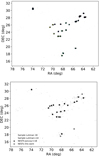 |
Fig. 11. Top: position map (RA, Dec) of the Taurus sample. Noise stars are depicted as grey small dots, while stars belonging to the structures found are shown as coloured squares, with different shades of purple, blue, yellow, and green representing different small scale structures. Bottom: comparison of the position of the NESTs found in J18 and those detected in this work. Grey triangles show the stars from the analysis of Luhman et al. (2010), while grey circles show stars in the updated samples from Luhman (2018). Black symbols mark the centroids of the NESTs detected: crosses the NESTs found in J18, and empty circles the NESTs found in this work. |
When we compare the results of the analysis of Taurus region (in Table 3) with those of synthetic regions (in Table 2), we observe an overall qualitative compatibility with significantly structured regions, that is, a large number of very compact (ρnom/ρCSR > 15) structures with a relatively low number of members (Nmax/Nmin = 5) is retrieved. However, the numerical indicators are different from the simple box fractal models studied in Sect. 3. The amount of NESTs, relative nominal density, the fraction of stars within them and the size of the most populated NEST compared to Nmin are larger in Taurus than in the fractal simulations. Our results indicate that even for an archetypically structured region, the nature of the structure is more complex than reflected by simple box-fractal models. This is consistent with the results from Lomax et al. (2018) and we throroughly analyse these findings in Appendix B.
4.2. IC 348
IC 348 is a SFR in the Perseus cloud, with YSOs of ages between 2 and 6 Myr and at a distance of 315 pc, according to Luhman et al. (2016), who provided an updated sample of its members. The general spatial trend of the YSO sample is clearly centrally concentrated, as can be seen in Fig. 12.
 |
Fig. 12. Position map (RA, Dec) of the IC 348 sample. Noise stars are depicted as grey dots, while stars belonging to the structures found are shown in colour. Each shade of purple, blue, and green represents a different NEST retrieved by S2D2. |
The initial sample contains 478 stars, whereas preprocessing (as explained in Sect. 2) found 13 binary systems, so the procedure was applied to a final sample of 465 stars. For this region (and also for Carina), densities and distances cannot be directly compared to other regions or to the simulated clusters due to the different physical size of the clusters.
Figure 12 shows a map with the detected structures, shown as coloured dots over the grey population. The general concentrated character of the region is in agreement with the value of Q = 0.97, consistent with a radial distribution with an exponent E = 2. We find six structures with ϵ = 0.0067 deg and Nmin = 5. Figure 12 shows a map of the YSOs in the sample, where coloured squares indicate belonging to a particular structure and Fig. 10 shows a histogram of the number of members in each NEST. The summarised results of the analysis of IC 348 are shown in Table 3. The fraction of stars in structures, fNEST, is close to distributions with significant central concentration (radial gradient with exponent E = 2). However, the relative maximum size of the structures, Nmax/Nmin is much smaller, suggesting less concentrated regions, with exponent E = 1. We note that in the centre of the cluster there are two substructures very close to each other, such that a small increase in the scale ϵ for DBSCAN would merge them within a larger single structure. This would decrease the significance of the NESTs, which is very high. The number of structures, Nstruct, or the relative nominal density for significant structures, may be coherent with both exponents, of either 1 or 2. These results indicate that the YSO distribution in IC 348 is reasonably well-represented by a radial density distribution with constant exponent between 1 and 2, and that the substructures found correspond to Poisson fluctuations at densities larger than ρCSR – and not to imprints of star formation sites.
4.3. Upper Scorpius
Upper Scorpius is a region of the Scorpius-Centaurus OB association, which is relatively close (∼145 pc) and young (∼11 Myr), according to Luhman et al. (2018), who also provided a rich, new catalogue of YSO members. A visual inspection of the sample indicates some non spherically symmetric concentration with some structure, or at least significant density variations within. This is compatible with the Q parameter of this sample Q = 0.915, which points to clear though mild concentration.
In general, our results (shown in Fig. 13) are compatible with moderate central concentration (radial with E = 1), although the amount of structure detected, or the fraction of stars within NESTs are more in agreement with greater spatial concentration. There is a large structure with 29 stars towards the north, and plenty of small scale structures dispersed through the region.
 |
Fig. 13. Position map (RA, Dec) of the Upper Scorpius sample. Noise stars are depicted as grey dots, while stars belonging to the structures found are shown in colour. Each shade of purple, blue, green, and yellow represents a different NEST retrieved by S2D2. |
Given the shape of the distribution, and the differences between radial and Plummer concentrated distributions, we believe that in this case we are dealing with a complex form of concentration with more than one slope, giving rise to a central density ‘plateau’. The situation is complex, and the small scale structures hard to interpret. There is a wide range of densities in the region, so a multi-scale analysis would shed light on the real nature and significance of these structures.
4.4. Carina
We finally apply our procedure to the YSOs in the Carina Nebula, a very large SFR with complex spatial structure (Fig. 14). It is known for hosting several open clusters (Trumpler 14, 15 and 16, Treasure Chest, and Bochum 11 in the window that we will analyse) and numerous massive stars, making it an interesting laboratory to studying massive star formation and its effects on the surrounding.
 |
Fig. 14. Position map (RA, Dec) of the Carina Nebula sample, comparing the results of S2D2 with those of B19 and K14. Dotted ellipses show the position of known clusters in the area, while black rimmed white ellipses show the structures obtained by Kuhn et al. (2014), tagged accordingly with letters. Noise stars are depicted as grey dots, the stars with significant clustering index I5 from Buckner et al. (2019) are coloured in red. Stars belonging to structures found by S2D2 are squares coloured following the same colour scheme as in Fig. 11, with different NESTS represented by different shades of purple, blue, yellow, and green. |
For this reason, the Carina SFR has been widely studied, which allows us to compare our results with two previous works. Carina was studied in Kuhn et al. (2014; henceforth K14) as part of the MYStIX survey, which also provided a catalogue of members used in this work. The authors retrieved structure using a parametric finite mixture model that fits isothermal ellipsoids to substructures. These structures are varied in terms of scale and density, although they are always of the same shape. The final parameters, such as the number of structures, are decided by comparing the results with different values in order to maximise the Akaike Information Criterium (which is proportional to the likelihood of the model and includes a penalty for its complexity, as explained in Feigelson & Babu 2012). A total of 20 subclusters were identified by K14.
The same sample from Carina was also recently studied by Buckner et al. (2019; henceforth B19) with the tool INDICATE, which is not a structure detection tool, but a diagnostic of the local clustering trends in a sample. INDICATE assesses the clustering tendency of each star in a sample and assigns it an index, where larger indices imply stars with a higher degree of spatial association. The index values are calibrated against random distributions to define a ‘significance threshold’ above which a star is considered to be spatially clustered.
In Fig. 14, the results from B19 and K14 are shown, and compared with those from S2D2. The stars with a clustering index from B19 above the significance level are shown in red. The structures found by K14 are depicted as black rimmed white ellipses labeled with letters, and black dotted ellipses show the known clusters in the area. The stars belonging to the different structures found by S2D2 are squares coloured following the same palette as in previous plots, with different shades of purple, green and yellow. The area of Trumpler 14 is zoomed so the retrieved NESTs are clearer.
The number of members of the structures found by S2D2 in Carina is shown in Fig. 10. In general, the structures retrieved by S2D2 are in agreement with previous works, with all of them in areas where the clustering index from B19 is significant and the majority (70%) of them in areas where K14 also found structures. We retrieved a large number of structures, mostly in the densest northern area, in the positions of Trumpler 14, 15, and 16. There are indications that the region is very complex in nature, with significant local radial concentrations, despite globally having a Q value indicating substructure. The ρCSR value of the region density is dominated by the northern area. The large value of Nmax/Nmin indicates that Trumpler 14, where a structure with more than 100 stars is retrieved with some associated secondary structures, is concentrated and shows a gradient. This is consistent with B19, where the highest index values are found, and also with the A and B structures in K14. Some small scale structure is detected in the Trumpler 15 and 13 areas, also consistent with previous work. In the northern region of Carina, the results given by the three methods are broadly compatible, with the exception of structure F given by K14. Here, no structure is retrieved by S2D2 since its density is more than a factor of two lower than the nominal density required for detection. The probability of structure F being an artefact due to random sampling or projection effects is not negligible. This is in agreement with B19 who found F had no stars with significant clustering tendencies and proposed it may not be real cluster but instead fluctuations in the dispersed population field. We therefore recommend great care when attempting to interpret this structure or including it in statistical analyses.
In the south, the only significant detection is a small structure in the Treasure Chest area, compatible with structure O from K14, and with significant clustering index according to B19. A comparison with previous work shows that we are losing some substructure due to the use of a single density (and thus, scale) for the whole region. The results given by B19 in the south also show low values for their clustering tendency compared to the northern area. K14 classified all the regions in the MYStIX catalogue according to the kind of substructure fitted by their method in four classes: ‘simple’ regions, with one single cluster; ‘cluster- halo’ regions, where a big structure surrounding a smaller, more compact one was identified; linear chain regions, where the subclusters were organised in filaments; and clumpy regions, where a large number of structures were found all over the area. Carina did not fit in any of these four categories, showing mixed traits, and was finally categorised as a complex region. This is consistent with our inability to detect all the structure in the complete region simultaneously. Additional tests with our procedure, separating the whole Carina region in south-east and north-west (using the same windows as in B19) show that separating the region before the analysis leads to similar results in the NW area, while in the SE area, more significant structure is retrieved – a result that is still globally compatible with the results of K14 and B19. To get all the significant structures at different scales at once, we recommend a multi-scale method, as that in Joncour (2019, in prep.).
5. Summary and conclusions
In this work, we present the S2D2 procedure, designed to systematically choose the parameters of ϵ (length scale) and Nmin (minimum number of points) based on the properties of the star sample, to guarantee that DBSCAN will search clusters for the smallest scale structures that are significant above random fluctuations. Different implementations of the procedure are to be made available for the scientific community.
We implemented S2D2 and tested it in both synthetic and real projected young clusters, representing a range of initial conditions at, and well beyond, the extent where these small-scale structures are present.
In substructured regions, S2D2 is very successful. The structure we retrieve is exactly what the method was designed for: very significant small-scale structures, or NESTs. In young SFRs such as Taurus, NESTs are candidates that are posed to serve as pristine remnants of the process of fragmentation of the original gas cloud and cores.
Even when we consider regions beyond the original scope of S2D2 (such as homogeneous clusters where the subclusters that we search for do not appear; or concentrated clusters that, in addition to having no subclusters, are not represented by a single density, ρCSR, to define the relevant scale and significance of the structures), the methodical and robust nature of our procedure gives consistent and systematic results.
Special care must be taken when interpreting the results of regions that are close to complete spatial randomness, characterised by values of the Q structure parameter in the range of Q ∈ (0.7, 0.87). In these cases, and despite retrieving only structures with more than 3-σ significance above random, we cannot guarantee that the structure retrieved, though compact and small-scale, is not associated to projection effects or the presence of a slight density gradient.
For concentrated regions, characterised by a large scale structure, the main core is detected accompanied by a halo of secondary structure. The appearance of secondary structures is one of the limitations of S2D2, as it is primarily an analysis that only considers a single scale or size as relevant. These structures appear in regions that are characterised by stellar density gradients and are associated to random fluctuations at different local densities.
Tests in real regions show that YSOs in observed SFRs hardly have such simple structures in idealised synthetic regions. In some cases, as shown in Carina, this is partly due to the choice of very large and complex regions, comprising several clusters of a simpler nature and possibly varied evolutionary states. However, disentangling these clusters into single samples can prove a very challenging task and the final sample size can be too small to significantly apply statistical methods to them.
The ideal method in those cases would consider the varied and complex nature of SFRs, analysing the structure at several scales. This way, the hierarchy of structures in terms of scale and density can be completely captured. For that reason, a multi-scale version of the procedure presented in this work is in development (Joncour, in prep.), with preliminary results shown in Joncour (2019).
The S2D2 provides consistent, robust, and meaningful detections of significant substructures in star-forming regions. As such, it allows for comparison of the structure in different regions. This work will be followed up by an extensive analysis of a whole set of observed SFRs in order to proceed to a statistical analysis of the retrieved substructures and assess their geometrical properties, as well as their evolutionary and dynamical status.
The Γ function is a special mathematical function that extends the factorial function for complex numbers, and as such, arises frequently in statistical calculations. For a complex number z with positive real part,  .
.
Acknowledgments
The Star Form Mapper project has received funding from the European Union’s Horizon 2020 research and innovation program under grant agreement No 687528.
References
- Aarseth, S. J., Tout, C. A., & Mardling, R. A. 2008, The Cambridge N-Body Lectures (Berlin, Heidelberg: Springer-Verlag), 760 [Google Scholar]
- Alfaro, E. J., & González, M. 2016, MNRAS, 456, 2900 [Google Scholar]
- Alfaro, E. J., & Román-Zúñiga, C. G. 2018, MNRAS, 478, L110 [Google Scholar]
- Allison, R. J., Goodwin, S. P., Parker, R. J., et al. 2009, MNRAS, 395, 1449 [Google Scholar]
- Astropy Collaboration (Robitaille, T. P., et al.) 2013, A&A, 558, A33 [NASA ADS] [CrossRef] [EDP Sciences] [Google Scholar]
- Baddeley, A., Rubak, E., & Turner, R. 2015, Spatial Point Patterns: Methodology and Applications with R (Chapman and Hall/CRC Press) [CrossRef] [Google Scholar]
- Baines, D., de Calle, I. L., Herrera-Fernandez, J. M., et al. 2019, in Astronomical Data Analysis Software and Systems XXVIII (Astronomical Society of the Pacific), ASP Conf. Ser., 523 [Google Scholar]
- Botev, Z. I., Grotowski, J. F., & Kroese, D. P. 2010, Ann. Stat., 38, 2916 [Google Scholar]
- Buckner, A. S. M., Khorrami, Z., Khalaj, P., et al. 2019, A&A, 622, A184 [NASA ADS] [CrossRef] [EDP Sciences] [Google Scholar]
- Cánovas, H., Cantero, C., Cieza, L., et al. 2019, A&A, 626, A80 [NASA ADS] [CrossRef] [EDP Sciences] [Google Scholar]
- Cantat-Gaudin, T., Jordi, C., Vallenari, A., et al. 2018, A&A, 618, A93 [NASA ADS] [CrossRef] [EDP Sciences] [Google Scholar]
- Cartwright, A. 2009, MNRAS, 400, 1427 [NASA ADS] [CrossRef] [Google Scholar]
- Cartwright, A., & Whitworth, A. P. 2004, MNRAS, 348, 589 [NASA ADS] [CrossRef] [Google Scholar]
- Cartwright, A., & Whitworth, A. P. 2009, MNRAS, 392, 341 [NASA ADS] [CrossRef] [Google Scholar]
- Casertano, S., & Hut, P. 1985, ApJ, 298, 80 [Google Scholar]
- Clarke, C. 2010, Philos. Trans. R. Soc. London Ser. A, 368, 733 [Google Scholar]
- Costado, M. T., Alfaro, E. J., González, M., & Sampedro, L. 2017, MNRAS, 465, 3879 [NASA ADS] [CrossRef] [Google Scholar]
- Daffern-Powell, E. C., & Parker, R. J. 2020, MNRAS, 493, 4925 [Google Scholar]
- Dib, S., Schmeja, S., & Parker, R. J. 2018, MNRAS, 473, 849 [NASA ADS] [CrossRef] [EDP Sciences] [Google Scholar]
- Diggle, P. J. 2003, Statistical Analysis of Spatial Point Patterns (New York: Wiley and Sons) [Google Scholar]
- Ester, M., Kriegel, H. P., Sander, J., & Xu, X. 1996, Proceedings of the Second International Conference on Knowledge Discovery and Data Mining, KDD’96 (AAAI Press), 226 [Google Scholar]
- Feigelson, E. D., & Babu, G. J. 2012, Modern Statistical Methods for Astronomy (Cambridge: Cambridge University Press) [Google Scholar]
- Fűrész, G., Hartmann, L. W., Szentgyorgyi, A. H., et al. 2006, ApJ, 648, 1090 [NASA ADS] [CrossRef] [Google Scholar]
- Fujii, M. S., & Portegies-Zwart, S. 2016, ApJ, 817, 4 [NASA ADS] [CrossRef] [Google Scholar]
- Gaia Collaboration (Prusti, T., et al.) 2016, A&A, 595, A1 [NASA ADS] [CrossRef] [EDP Sciences] [Google Scholar]
- Gomez, M., Hartmann, L., Kenyon, S. J., & Hewett, R. 1993, AJ, 105, 1927 [NASA ADS] [CrossRef] [Google Scholar]
- González, M., & Alfaro, E. J. 2017, MNRAS, 465, 1889 [NASA ADS] [CrossRef] [Google Scholar]
- Gutermuth, R. A., Megeath, S. T., Myers, P. C., et al. 2009, ApJS, 184, 18 [NASA ADS] [CrossRef] [Google Scholar]
- Hacar, A., Tafalla, M., & Alves, J. 2017, A&A, 606, A123 [NASA ADS] [CrossRef] [EDP Sciences] [Google Scholar]
- Hetem, A., & Gregorio-Hetem, J. 2019, MNRAS, 490, 2521 [Google Scholar]
- Illian, J., Penttinen, A., Stoyan, H., & Stoyan, D. 2008, Statistical Analysis and Modelling of Spatial Point Patterns (Hoboken: John Wiley and Sons, Ltd) [Google Scholar]
- Jaffa, S. E., Whitworth, A. P., & Lomax, O. 2017, MNRAS, 466, 1082 [NASA ADS] [CrossRef] [Google Scholar]
- Joncour, I. 2019, in Multiscale Spatial Analysis of Young Stars Complex using the dbscan Clustering Algorithm, eds. P. J. Teuben, M. W. Pound, B. A. Thomas, & E. M. Warner, ASP Conf. Ser., 523, 87 [Google Scholar]
- Joncour, I., Duchêne, G., & Moraux, E. 2017, A&A, 599, A14 [NASA ADS] [CrossRef] [EDP Sciences] [Google Scholar]
- Joncour, I., Duchêne, G., Moraux, E., & Motte, F. 2018, A&A, 620, A27 [NASA ADS] [CrossRef] [EDP Sciences] [Google Scholar]
- Joncour, I., Buckner, A., Khalaj, P., Moraux, E., & Motte, F. 2020, ArXiv e-prints [arXiv:2006.07830] [Google Scholar]
- Kenyon, S. J., Gómez, M., & Whitney, B. A. 2008, in Low Mass Star Formation in the Taurus-Auriga Clouds, ed. B. Reipurth, 4, 405 [Google Scholar]
- Kirk, H., & Myers, P. C. 2011, ApJ, 727, 64 [NASA ADS] [CrossRef] [Google Scholar]
- Kirk, H., Johnstone, D., Di Francesco, J., et al. 2016, ApJ, 821, 98 [Google Scholar]
- Kounkel, M., & Covey, K. 2019, AJ, 158, 122 [Google Scholar]
- Kraus, A. L., & Hillenbrand, L. A. 2008, ApJ, 686, L111 [NASA ADS] [CrossRef] [Google Scholar]
- Kuhn, M. A., Feigelson, E. D., Getman, K. V., et al. 2014, ApJ, 787, 107 [Google Scholar]
- Küpper, A. H. W., Maschberger, T., Kroupa, P., & Baumgardt, H. 2011, MNRAS, 417, 2300 [NASA ADS] [CrossRef] [Google Scholar]
- Larson, R. B. 1995, MNRAS, 272, 213 [NASA ADS] [Google Scholar]
- Larson, R. B. 2007, Rep. Progr. Phys., 70, 337 [CrossRef] [Google Scholar]
- Lomax, O., Bates, M. L., & Whitworth, A. P. 2018, MNRAS, 480, 371 [Google Scholar]
- Luhman, K. L. 2018, AJ, 156, 271 [NASA ADS] [CrossRef] [Google Scholar]
- Luhman, K. L., Allen, P. R., Espaillat, C., Hartmann, L., & Calvet, N. 2010, ApJS, 186, 111 [NASA ADS] [CrossRef] [Google Scholar]
- Luhman, K. L., Esplin, T. L., & Loutrel, N. P. 2016, ApJ, 827, 52 [NASA ADS] [CrossRef] [Google Scholar]
- Luhman, K. L., Herrmann, K. A., Mamajek, E. E., Esplin, T. L., & Pecaut, M. J. 2018, AJ, 156, 76 [NASA ADS] [CrossRef] [Google Scholar]
- Maíz-Apellániz, J., Pérez, E., & Mas-Hesse, J. M. 2004, AJ, 128, 1196 [NASA ADS] [CrossRef] [Google Scholar]
- Maschberger, T., & Clarke, C. J. 2011, MNRAS, 416, 541 [Google Scholar]
- Parker, R. J. 2018, MNRAS, 476, 617 [Google Scholar]
- Parker, R. J., & Dale, J. E. 2013, MNRAS, 432, 986 [NASA ADS] [CrossRef] [Google Scholar]
- Parker, R. J., & Goodwin, S. P. 2015, MNRAS, 449, 3381 [NASA ADS] [CrossRef] [Google Scholar]
- Parker, R. J., & Meyer, M. R. 2012, MNRAS, 427, 637 [Google Scholar]
- Parker, R. J., & Wright, N. J. 2018, MNRAS, 481, 1679 [Google Scholar]
- Parker, R. J., Wright, N. J., Goodwin, S. P., & Meyer, M. R. 2014, MNRAS, 438, 620 [NASA ADS] [CrossRef] [Google Scholar]
- Pedregosa, F., Varoquaux, G., Gramfort, A., et al. 2011, J. Mach. Learn. Res., 12, 2825 [Google Scholar]
- Peebles, P. J. E. 1980, Ninth Texas Symposium on Relativistic Astrophysics, 336, 161 [Google Scholar]
- Pfalzner, S., Kaczmarek, T., & Olczak, C. 2012, A&A, 545, A122 [NASA ADS] [CrossRef] [EDP Sciences] [Google Scholar]
- Pflamm-Altenburg, J., & Kroupa, P. 2008, Nature, 455, 641 [NASA ADS] [CrossRef] [PubMed] [Google Scholar]
- Pilbratt, G. 2010, JENAM 2010, Joint European and National Astronomy Meeting, 149 [Google Scholar]
- Reiter, M., & Parker, R. J. 2019, MNRAS, 486, 4354 [CrossRef] [Google Scholar]
- Retter, B., Hatchell, J., & Naylor, T. 2019, MNRAS, 487, 887 [Google Scholar]
- Robitaille, J. F., Motte, F., Schneider, N., Elia, D., & Bontemps, S. 2019, A&A, 628, A33 [CrossRef] [EDP Sciences] [Google Scholar]
- Robitaille, J.-F., Abdeldayem, A., Joncour, I., et al. 2020, A&A, 641, A138 [CrossRef] [EDP Sciences] [Google Scholar]
- Sacco, G. G., Spina, L., Randich, S., et al. 2017, A&A, 601, A97 [NASA ADS] [CrossRef] [EDP Sciences] [Google Scholar]
- Sánchez, N., & Alfaro, E. J. 2009, ApJ, 696, 2086 [NASA ADS] [CrossRef] [Google Scholar]
- Schmeja, S., & Klessen, R. S. 2006, A&A, 449, 151 [NASA ADS] [CrossRef] [EDP Sciences] [Google Scholar]
- Siemiginowska, A., Eadie, G., Czekala, I., et al. 2019, BAAS, 51, 355 [Google Scholar]
- Sills, A., Rieder, S., Scora, J., McCloskey, J., & Jaffa, S. 2018, MNRAS, 477, 1903 [NASA ADS] [CrossRef] [Google Scholar]
- Silverman, B. W. 1986, Density Estimation for Statistics and Data Analysis (London: Chapman and Hall) [Google Scholar]
- Vermeesch, P., Resentini, A., & Garzanti, E. 2016, Sediment. Geol., 336, 14 [Google Scholar]
- Wright, N. J., Parker, R. J., Goodwin, S. P., & Drake, J. J. 2014, MNRAS, 438, 639 [NASA ADS] [CrossRef] [Google Scholar]
Appendix A: Public implementations of S2D2
The development of this work is part of the StarFormMapper EU project, which is meant to provide the community with different tools and materials for studying the spatial distribution of young stars in SFRs and thus constrain the star formation process.
In the following, we present the implementations of the procedure that are available for the community. These make use of different software packages: scikit.learn and astropy in python (Pedregosa et al. 2011; Astropy Collaboration 2013), and spatstat in R (Baddeley et al. 2015). In the StarFormMapper web page3, updated links to the implementations of the procedure will be available, each with its own user guide.
A.1. Basic users: DEAVI
One of the milestones of StarFormMapper is DEAVI, (Baines et al. 2019), an added value interface to manage and exploit data from the Gaia and Herschel missions, which is in final development and will be presented and publicly available during 20204. In addition to Gaia and Herschel data, DEAVI will provide simulations of the stellar and gas component of SFRs, and several tools of analysis, including S2D2 and INDICATE (B19).
The S2D2 interface in DEAVI is very simple, allowing any user to apply S2D2 without the need to compile or install anything. Due to its simplicity, the default procedure will be very conservative so relevance of the structures detected is ensured. By default, the confidence level for structure detection will be fixed at 99.85% and the complete procedure (calculating ϵ and Nmin and retrieving the structures) will only be applied to regions where we can guarantee that there is a global structure. This will be done by requiring that the Q structure parameter (CW04) is below 0.8. Not only that, if Q is larger than 0.7, the program output will include a warning so the user is cautious with the interpretation of the structures retrieved. The motivation behind these limitations is explained in the text: in particular, in Sect. 3 and summarised in Sect. 5.
We are aware that these conditions can be too strict for some applications, so we also allow users to manually introduce ϵ and Nmin values to apply DBSCAN and analyse regions with larger Q values, with the aim of either retrieving structures of different sizes or based on lower levels of confidence.
A.2. Advanced usage: GitHub
We also provide the community with GitHub repositories with python5 and R6 complete implementations of the procedure for more advanced users who want to have more control on the procedure. In these implementations, the user will be able to modify a parameter file containing all the options available to DEAVI users and, additionally, the Q limit for performing the analysis, and the significance limit for structure detection. In the GitHub repositories, the whole code will be available, so further modifications of the procedure will be possible.
Appendix B: Measuring the structure of stellar clusters: limits and extensions of the Q parameter
Even though defining and quantifying the level and nature of structure of a region is beyond the main objectives of this work, it is clearly related. In this appendix we review the currently most popular method to evaluate the structure of star-forming regions: the Q parameter, used in this work. We will discuss its underlying model, assumption and limits, along with two recent extensions/alternatives to Q, namely Q+ by Jaffa et al. (2017; henceforth JF17), and ClusterFrac, by Lomax et al. (2018; henceforth LX18).
B.1. Q parameter
The Q parameter was introduced in CW04, and utilises central values of the edge length distribution of the complete graph (CG) and minimum spanning tree (MST) to describe the spatial structure of a point distribution, allowing to distinguish between substructured, homogeneous and concentrated distributions. This was a feat, since CG and MST distributions separately do give a different signal for clustered, homogeneous and inhibited distributions (where these definitions are in comparison to homogeneous, as explained in the main text, in Sect. 2.2), but they cannot distinguish if a clustered distribution has only one mode, as in a concentrated distribution, or several.
We recall that  is the ratio between the normalised mean length of the MST
  , and that of the complete graph,
  , making it a scale-free parameter. In the original work by CW04, the Q parameter was calibrated with synthetic clusters from the box-fractal and radial families, as those used in this work, ranging from very substructured to very concentrated regimes and testing both the fractal and radial approximation to a homogeneous distribution. They found that homogeneous distributions had Q ∼ 0.8, fractals were characterised by lower Q values, and radials by larger Q. In a later work, Cartwright (2009) searched for a similar pattern for clusters taking into account kinematical information, but found that including velocity in the calculations did not improve the discriminant power of Q.
A constant value of Q = Q0, such as the threshold 0.8 found to separate fractal from radial distributions, corresponds to a line in the ( ,
,  ) 2D space passing by the origin with slope Q0. The position of clusters in this space has also been used to characterise the structure of clusters, in a variety of works, such as Cartwright (2009), Parker & Dale (2013); LX18; Daffern-Powell & Parker (2020), and references therein. In Fig. B.1, the positions of the distributions analysed in this work are shown in the (
 ,
,  ) space. In the upper panel of Fig. B.1, the normalisation used is the standard one, taken from CW04, which uses the maximum radius and the area of the circle corresponding to that radius to normalise the MST and CG mean values. The lower panel shows the results of the Schmeja & Klessen (2006) normalisation, which uses the area of the convex hull of the point distribution and the radius of the equivalent circle to normalise. We note that both of these normalisations produce the same Q values, although the differences in the (
 ,
,  ) space are obvious from the plot. This was explored in Parker (2018), along with a different normalisation proposed by Kirk et al. (2016), where the area of the convex hull was used but its radius was calculated as the maximum distance from the mean position to the most distant point in the hull. Parker (2018) concluded that this distorted the
  ,
,  , and Q values to the point that the Q = 0.8 limit was not valid anymore. The Schmeja & Klessen (2006) normalisation is more robust to the presence of outliers in the (
 ,
,  ) space, effectively confining the fractal distributions, which naturally have strong dispersion to smaller regions of the (
 ,
,  ) plane. This was shown in the appendix of Parker & Goodwin (2015). This highlights the differences between the substructured real regions (Carina and Taurus), and the fractal distributions, that were not that obvious with the original CW04 normalisation.
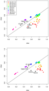 |
Fig. B.1.
|
The original Q definition assumes the spherical symmetry of the clusters. Cartwright & Whitworth (2009) explore the effect of elongation, which they calculate as the ratio of the extent of the data in the direction maximising that extent and the perpendicular one. Schmeja & Klessen (2006) propose an alternate definition for the elongation based on the ratio between the areas of the maximum distance circle and that of the convex hull. Cartwright & Whitworth (2009) concluded that even though elongation modified the Q values, the effect for moderate elongations (on the order of or less than 3) was within the uncertainty ranges of Q for spherically symmetrical clusters. For larger elongations, they calculated a table of corrections.
Cartwright & Whitworth (2009) warned that the values of both Q and the elongation would be affected by the presence of outliers. This was explored in Chameleon I by Sacco et al. (2017), where they not only use jackknife resampling to estimate the uncertainty of the Q value, but they also calculate the Q parameter of different subsamples restricted to the central areas of the cluster. They showed that even though the Q of the central subsample indicated a strong substructure, including the outer part increased it to values typical of homogeneous distributions.
One of the main advantages of the Q parameter, already highlighted in CW04, is that it can trace all the way to to a fractal dimension or a radial exponent, in the box-fractal or radial paradigm, and that this estimate is robust even for small samples (Nstar ∼ 100). This was confirmed with further numerical experiments by Sánchez & Alfaro (2009), who found that, even if the calculation of the fractal dimension using the two point correlation function (TPCF, as defined in the text, in Sect. 2.2) was in general more exact, it was not reliable for Nstar < 200. They also found that the Q estimate varied with the number of points, lowering the threshold separating substructured from concentrated regions from 0.8 to 0.785. Parker & Dale (2013) expanded the study of the variation of Q with the number of members in a region, and also tested a variety of synthetic and more complex cases, such as masking a region of a sample to produce a hole or combining different synthetic regions of different characteristics in a single sample. The general behaviour of the Q becomes, in those cases, very hard to predict.
B.2. Expanding the box-fractal model: Q+
JF17 expand the simple box-fractal model used in CW04 to one with two additional parameters (the length scale L and the volume-density exponent C) to generate more realistic fractal models. The model is still box fractal, since it is based on the subsequent subdivision of a box, the root cube, where only a fixed proportion of the new smaller boxes are fertile and keep being divided. The star distribution is finally created by generating points in the fertile areas of the original box.
-
The fractal dimension, D, with the same meaning as in CW04, where D is related indicates to the probability of cubes in each division to be fertile Pfertile = 2D − Dim, where Dim is the dimension of the space. Increasing D increases the filling factor of a cluster, having more fertile cubes, and the number of stars.
-
The length scale, L, is associated to the number of levels, l, which indicates the finite spatial range of scales associated to the fractal through the relationship 2L = R, where R is the ratio between the size of cubes in the last level and the root cube. Increasing L increases R the relative size of the smallest separations compared to the size of the cluster and the number of stars.
-
The volume density scaling exponent, C, is associated to the degree of concentration in the smallest scales. The additional volume density in level l is δnl = n02C, with n0 the density of the root cube. Increasing C concentrates stars in the smaller structures, decreasing the number of stars.
Within that paradigm, the CW04 fractal clusters as the ones used in this work have D = D,  , and C = ∞. When generating a JF17 fractal cluster with a specific set of D, L, C, the number of members cannot be prefixed.
JF17 calculate, for each synthetic cluster, a set of seven features describing the characteristics of the cluster and based on the MST and CG of the distribution. Based on these features, they perform simulations varying D, L, and C to which they apply principal component analysis (PCA), obtaining a 2D principal component (PC) space on which they estimate the values for D and L. C is estimated independently using a bayesian approach. The results obtained by JF17 in simulations of their fractal models are very good, except for C = ∞, which is not well-constrained. Even in the PC space, the effect of C is hard to disentangle from that of D and L. In real regions, they obtain estimates of the fractal dimension which are systematically lower, but follow the same trend as previous estimates using the standard Q parameter. JF17 also report that clusters with D > 2.32 will appear smooth.
Figures B.2 and B.3 show the results of the Q+ algorithm (from the author’s github python implementation, provided in JF17) on our simulated clusters. We only applied the code to the fractal distributions and the homogeneous radial approximation since concentrated distributions are beyond their scope and the user is warned when introducing a distribution with Q ≧ 0.9. From the top panel in Fig. B.2, it is clear that the standard Q estimates for the fractal dimension are much better than those provided by Q+, which is not surprising since the clusters were generated as simple box-fractal models following CW04’s recipe. As for the Q+ estimates in our synthetic clusters, they are always lower than the values obtained from the simple Q, and they do not help in distinguishing fractals with dimension 1.6 from fractals with dimension 2, or fractals with D = 2.6 from homogeneous distributions. The bottom plot in Fig. B.2 shows the L estimates, which have similar problems as those of D: they all overlap, and they cannot discriminate amongst distributions. In addition they are systematically overestimated.
 |
Fig. B.2. Fractal dimension estimated using the standard Q approach from CW04 (stars), and the Q+ from JF17 (black rimmed coloured dots) against the fractal dimension used to generate the clusters. Bottom: estimated against theoretical value of L for the simulated clusters considered in this work. Each colour represents a different true fractal dimension. The black line is the identity function, where the theoretical and estimated values are equal. Please note that the Fractal with D = 3 and the radial with E = 0 both represent a homogeneous distribution, and that some of the D estimates and all the L estimates given by Q+ overlap. |
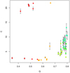 |
Fig. B.3. Estimated value of C for the simulated clusters. The colour code is the same as in Fig. B.2. |
Figure B.3 shows the values of C estimated with Q+ vs their standard Q parameter. As already indicated in JF17, the values are not well-constrained, and in fact, a significant amount of the distributions tested have C < 5, which are not good estimates considering that the theoretical value is =∞. We note that JF17 remarked that the Q+ estimates will improve as the number of simulations for the PCA and Bayesian calculations is increased, better sampling the (D, L, C) space. We conclude that, at least in its current state, a Q+ analysis does not improve the simple Q analysis for the box-fractal models, as those in this work.
B.3. Fractal Brownian model: ClusFrac
LX18 extend the complete box-fractal/radial paradigm (not just the fractal part of it, as in JF17), to cover a much larger part of the ( ,
,  ) space, filling, in particular, the areas usually occupied by real clusters, as shown in the lower plot of Fig. B.1.
The fractal Brownian model clusters start from a fractal Brownian model (FBM), usually used for describing the structure of clouds, with fixed drift exponent H, which is related to the fractal dimension of the cloud and the slope of its Fourier power spectrum. The cloud field f(r, H) is obtained as the inverse Fourier transform of its power spectrum. After filtering for the smallest spatial scales of self similarity, the cloud is then exponentiated with parameter σ, transforming the Gaussian distribution into a lognormal:
 (B.1)
(B.1)
This lognormal field will be used as the probability density function to sample stars and build clusters, and H, σ are its parameters. For fixed H, varying σ changes the dynamic range of the cloud. This lognormal cloud fulfils the conditions to be a probability density function, from which the stars are sampled.
LX18 simulated a variety of FBM clusters with different random seeds and values of H and σ, finding that there is an anticorrelation between  and σ, and that clusters with H = 1 fulfil the same role as radials.
To estimate H and σ LX18 fit artificial neural network regressors (ANNs, specifically multilayer perceptrons with one hidden layer) using as features the MST and CG edge length distribution moments (from the first to the fourth) after whitening the clusters (rescaling and eliminating elongation). They trained 3 ANNs, each of which fit clusters with different population ranges (rNstar < 99, 100 < Nstar < 315, and 316 < Nstar < 999). Their test results are very good in artificial FBM clusters, particularly when they are well-populated. The results in observed clusters are hard to evaluate: we get some values for H and σ, but their meaning is not clear: in looking at them, we cannot say whether the distribution is clumpy or not. This means that we cannot rule out the possibility that FBM clusters are overfitted by the ANNs, in which case results of clusters that do not follow a FBM could be unreliable. Overfitting can be of importance since the exponentiated fractal Brownian model is not a complete descriptor of the interstellar medium (see e.g., Robitaille et al. 2020, and references therein).
We cannot directly calculate and compare values of H and σ that would correspond to our clusters, but LX18 warn that H, even though it is related to the fractal dimension, must be taken with caution, since with the effect of sigma does not necessarily correspond with what we consider to be clumpy. Despite the great advantage in describing clusters with parameters and models that can be applied to the gas component of SFRs, H and σ are still a bit obscure, and somehow lack intuitive descriptive power. This can be due simply to their novelty, so more theoretical and applied studies of the FBM should be done to deepen our understanding of H and σ and better interpret them.
Appendix C: One point correlation function and simulations
We show the general behaviour of the OPCF in simulated clusters, supporting the results presented in the main text. We recall that OPCF stands for the one point correlation function Ψ(r) introduced in J17, which compares the first nearest neighbour distance distribution of the sample with that of a theoretical homogeneous random distribution. The OPCF is used by S2D2 to calculate ϵ, the relevant scale to search for small, significant substructure, as described in Sect. 2.2 in the main text; and ϵ is the smallest distance where the OPCF crosses the 1 boundary decreasingly, separating the excess (with respect to random) of stars with nearest neighbour at smaller r and depletion at larger.
First of all, in Fig. C.1 we show the ϵ values obtained using Silverman’s formula to calculate the bandwidth for the Gaussian kernel against the ϵ obtained with Botev’s algorithm (Botev et al. 2010). As described in Sect. 2.2, this Gaussian kernel is used to calculate the distribution of the first nearest neighbour distance in the sample. Botev’s algorithm is complex and based on diffusion equations. We use the R package provenance (Vermeesch et al. 2016) to calculate the bandwidth.
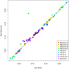 |
Fig. C.1. ϵ value obtained by S2D2 when the OPCF is generated using Botev’s algorithm (Botev et al. 2010) instead of Silverman’s formula (Silverman 1986) for the bandwidth. |
Both approaches give similar results, with a very significant difference only in one realisation of a fractal approximation to a homogeneous distribution (D = 3), where the dispersion of the ϵ values is large due to the closeness of the first nearest neighbour distribution to the theoretical homogeneous one. The shape of the OPCF in this case is shown in Fig. C.3.
Each panel in Figs. C.2–C.4 summarises the OPCF values for the fractal, homogeneous, and concentrated distributions in this work (see Table 1). For each distribution, the black lines show the quartiles Q1 and Q3 of the OPCF at each distance, the interquartile area is shaded in blue, and the red line shows its median value. The theoretical value of the OPCF at a random homogeneous distribution (which would be a function with constant value 1) is shown as a black horizontal dashed line, and the mean value of ϵ calculated by S2D2 (also shown in Table 2) is shown as a green vertical dashed line.
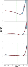 |
Fig. C.2. Top: median value of the OPCF at each distance for 10 realisations of a fractal distribution with D = 1.6 in red. Black solid lines represent the quartiles Q1 and Q3, with the inter-quartile range area shaded in blue. The horizontal dashed black line at constant value 1 represents the theoretical value for CSR, and the vertical dashed green line shows the average value of the ϵ obtained by S2D2 (see Table 2). Middle: same for a fractal distribution with D = 2.0. Bottom: same for a fractal distribution with D = 2.6. |
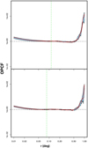 |
Fig. C.3. Top: plot analogous to that in Fig. C.2, summarising the OPCF in a fractal with D = 3.0. Bottom: same for a Radial with E = 0.0. |
 |
Fig. C.4. Plot analogous to that in Fig. C.2, summarising the OPCF for concentrated distributions. From left to right and top to bottom: radial distribution with exponent E = 1, radial distribution with exponent E = 2, radial distribution with exponent E = 2.5, and Plummer distribution. |
Even though there are differences amongst distributions, the use of the OPCF by itself to determine the structure of a point pattern is limited. This is partially due to the fact that it is based on the first nearest neighbour and only measures first order effects. This is similar to the lack of discriminant power between substructured and concentrated distributions associated to the MST distribution, as described in Appendix B from CW4. In their work, they include second order effects through the distance distribution of the sample, defining the Q parameter. The Q parameter has been thoroughly described in Appendix B, but we remind the reader that it is a global quantity, normalised to account for the size of the region.
Both substructured and concentrated distributions are clustered compared to CSR. This is evident in Figs. C.2 and C.4, where a pattern on the characteristics of stars with respect to random associated to distance can be seen (as in e.g., J17). This pattern consists in an excess of close stars compared to random expectation at small distances (shown by an OPCF larger than one), followed by the depletion of stars with a first nearest neighbour at intermediate distances and an excess at larger distances. In both cases, the closer a distribution is to CSR, the closer the OPCF values get to 1, with both the fractal and radial distributions converging towards the theoretical homogeneous case of Ψ(r) = 1, as shown in Fig. C.3. We note that for a homogeneous distribution, the values of the OPCF are close to unity in a significant part of its domain. As explained in the text, this results in the ϵ obtained by S2D2, having very different values based on random sampling effects.
All Tables
Spatial distributions, with parameters and references used to generate synthetic clusters.
Sample mean ± sample standard deviation of the procedure results in synthetic clusters, grouped by distribution.
All Figures
 |
Fig. 1. Application of DBSCAN algorithm to an example sample. Each panel represents one step in the process, with panel 4 showing the final result of the algorithm. The grey dots represent points that are not assigned to any cluster (noise points in panel 4), while the coloured, big dots depict points assigned to clusters (C1, C2, and C3) and each cluster is represented with a different colour. Coloured points with a black border are core points in a cluster, while those without one represent border points. Black circles show the ϵ environment of some representative points, which are also labeled. First panel: depicts the detection of a cluster within the sample. The ϵ-vicinity of the point labeled as p has more than Nmin = 5 sample members within, so p is identified as a core point (represented as a black-edged, coloured point) of the first identified cluster, C1, and the points within its ϵ-neighbourhood are marked as blue, since they are directly reachable from p and, thus, belong to the cluster C1. A subsequent step is to check the ϵ-vicinities of these points belonging to C1, which leads to the discovery of new members of C1, and the classification of some of them as core points. Bottom left panel: a latter epoch in the algorithm application, where a second cluster C2 composed only of core points is identified. Last panel: final results of the algorithm, where a third cluster, C3, with a single core point, is identified. The point q is in the ϵ-vicinities of core points in C1 and C3, so it will be assigned to either cluster depending on the processing order of the points. |
| In the text | |
 |
Fig. 2. Example realisation of each of the distributions in Table 1. |
| In the text | |
 |
Fig. 3. Density against the Q structure parameter for all synthetic regions. Different symbols indicate whether the parent distribution is fractal or radial, while colour indicates a different parent distribution. |
| In the text | |
 |
Fig. 4. Top: ϵ scale parameter for DBSCAN calculated with the procedure presented in Sect. 2.2 against Q structure parameter. Middle: relative nominal density of the detected structures ( |
| In the text | |
 |
Fig. 5. Number of structures detected with the procedure against Q structure parameter. Colours and symbols represent parent distributions, with the same colour and symbol code as in Fig. 3. |
| In the text | |
 |
Fig. 6. Top: fraction of stars in NESTs against Q structure parameter. Bottom: relative maximum size of structure detected Nmax weighted by the significant number of points Nmin against Q structure parameter. Colours and symbols represent parent distributions, with the same code as in Fig. 3. |
| In the text | |
 |
Fig. 7. Top: map of structures in a fractal with D = 1.6. Middle: same for a fractal with D = 2.0. Bottom: same for a fractal with D = 2.6. Noise stars are in grey, while stars in structures are shown as coloured squares. Each shade of purple, blue, green, and yellow represents a different small-scale structure retrieved by S2D2. |
| In the text | |
 |
Fig. 8. Top: map of structures in a fractal with D = 3.0. Bottom: same for a radial with E = 0.0. Noise stars are in grey, while the purple squares in the lower plot belong to a significant structure retrieved by the procedure. |
| In the text | |
 |
Fig. 9. Maps with the structures found using the procedure, e.g., simulations drawn from concentrated distributions. From left to right and top to bottom: radial with exponent E = 1.0, radial with E = 2.0, radial with E = 2.5, and Plummer, respectively. Noise stars are represented as grey dots, while the stars belonging to substructures are squares coloured in different shades of blue, purple, green, and yellow according to the small scale structure that they belong to. We note that only the central area of the clusters is shown, so the retrieved substructure is clearer. |
| In the text | |
 |
Fig. 10. Histogram of the number of members of the NESTs found in the observed regions. |
| In the text | |
 |
Fig. 11. Top: position map (RA, Dec) of the Taurus sample. Noise stars are depicted as grey small dots, while stars belonging to the structures found are shown as coloured squares, with different shades of purple, blue, yellow, and green representing different small scale structures. Bottom: comparison of the position of the NESTs found in J18 and those detected in this work. Grey triangles show the stars from the analysis of Luhman et al. (2010), while grey circles show stars in the updated samples from Luhman (2018). Black symbols mark the centroids of the NESTs detected: crosses the NESTs found in J18, and empty circles the NESTs found in this work. |
| In the text | |
 |
Fig. 12. Position map (RA, Dec) of the IC 348 sample. Noise stars are depicted as grey dots, while stars belonging to the structures found are shown in colour. Each shade of purple, blue, and green represents a different NEST retrieved by S2D2. |
| In the text | |
 |
Fig. 13. Position map (RA, Dec) of the Upper Scorpius sample. Noise stars are depicted as grey dots, while stars belonging to the structures found are shown in colour. Each shade of purple, blue, green, and yellow represents a different NEST retrieved by S2D2. |
| In the text | |
 |
Fig. 14. Position map (RA, Dec) of the Carina Nebula sample, comparing the results of S2D2 with those of B19 and K14. Dotted ellipses show the position of known clusters in the area, while black rimmed white ellipses show the structures obtained by Kuhn et al. (2014), tagged accordingly with letters. Noise stars are depicted as grey dots, the stars with significant clustering index I5 from Buckner et al. (2019) are coloured in red. Stars belonging to structures found by S2D2 are squares coloured following the same colour scheme as in Fig. 11, with different NESTS represented by different shades of purple, blue, yellow, and green. |
| In the text | |
 |
Fig. B.1.
|
| In the text | |
 |
Fig. B.2. Fractal dimension estimated using the standard Q approach from CW04 (stars), and the Q+ from JF17 (black rimmed coloured dots) against the fractal dimension used to generate the clusters. Bottom: estimated against theoretical value of L for the simulated clusters considered in this work. Each colour represents a different true fractal dimension. The black line is the identity function, where the theoretical and estimated values are equal. Please note that the Fractal with D = 3 and the radial with E = 0 both represent a homogeneous distribution, and that some of the D estimates and all the L estimates given by Q+ overlap. |
| In the text | |
 |
Fig. B.3. Estimated value of C for the simulated clusters. The colour code is the same as in Fig. B.2. |
| In the text | |
 |
Fig. C.1. ϵ value obtained by S2D2 when the OPCF is generated using Botev’s algorithm (Botev et al. 2010) instead of Silverman’s formula (Silverman 1986) for the bandwidth. |
| In the text | |
 |
Fig. C.2. Top: median value of the OPCF at each distance for 10 realisations of a fractal distribution with D = 1.6 in red. Black solid lines represent the quartiles Q1 and Q3, with the inter-quartile range area shaded in blue. The horizontal dashed black line at constant value 1 represents the theoretical value for CSR, and the vertical dashed green line shows the average value of the ϵ obtained by S2D2 (see Table 2). Middle: same for a fractal distribution with D = 2.0. Bottom: same for a fractal distribution with D = 2.6. |
| In the text | |
 |
Fig. C.3. Top: plot analogous to that in Fig. C.2, summarising the OPCF in a fractal with D = 3.0. Bottom: same for a Radial with E = 0.0. |
| In the text | |
 |
Fig. C.4. Plot analogous to that in Fig. C.2, summarising the OPCF for concentrated distributions. From left to right and top to bottom: radial distribution with exponent E = 1, radial distribution with exponent E = 2, radial distribution with exponent E = 2.5, and Plummer distribution. |
| In the text | |
Current usage metrics show cumulative count of Article Views (full-text article views including HTML views, PDF and ePub downloads, according to the available data) and Abstracts Views on Vision4Press platform.
Data correspond to usage on the plateform after 2015. The current usage metrics is available 48-96 hours after online publication and is updated daily on week days.
Initial download of the metrics may take a while.


