| Issue |
A&A
Volume 688, August 2024
|
|
|---|---|---|
| Article Number | A224 | |
| Number of page(s) | 10 | |
| Section | Interstellar and circumstellar matter | |
| DOI | https://doi.org/10.1051/0004-6361/202450830 | |
| Published online | 26 August 2024 | |
Cloud structure and young star distribution in the Dragonfish complex★
1
Universidad Internacional de Valencia (VIU),
C/Pintor Sorolla 21,
46002
Valencia, Spain
e-mail: nmsáThis email address is being protected from spambots. You need JavaScript enabled to view it.
2
Departament d’Astronomia i Astrofísica, Universitat de València,
Burjassot,
46100, Spain
Received:
22
May
2024
Accepted:
3
July
2024
Abstract
Context. Star formation is a complex process involving several physical mechanisms that interact with each other at different spatial scales. One way to shed some light on this process is to analyse the relation between the spatial distributions of gas and newly formed stars. In order to obtain robust results, it is necessary for this comparison to be made using quantitative and consistent descriptors that are applied to the same star-forming region.
Aims. We used fractal analysis to characterise and compare in a self-consistent way the structure of the cloud and the distribution of young stellar objects (YSO) in the Dragonfish star-forming complex.
Methods. Different emission maps of the Dragonfish nebula were retrieved from the NASA/IPAC Infrared Science and the Planck Legacy archives. Moreover, we used photometric information from the AllWISE catalogue to select a total of 1082 YSOs in the region. We derived the physical properties for some of these from their spectral energy distributions (SEDs). For the cloud images and YSOs, the three-dimensional fractal dimension (Df) was calculated using previously developed and calibrated algorithms.
Results. The fractal dimension of the Dragonfish nebula (Df = 2.6–2.7) agrees very well with values previously obtained for the Orion, Ophiuchus, and Perseus clouds. On the other hand, YSOs exhibit a significantly lower value on average (Df = 1.9–2.0), which indicates that their structure is far more clumpy than the material from which they formed. Younger Class I and Class II sources have lower values (Df = 1.7 ± 0.1) than more evolved transition disk objects (Df = 2.2 ± 0.1), which shows a certain evolutionary effect according to which an initially clumpy structure tends to gradually disappear over time.
Conclusions. The structure of the Dragonfish complex is similar to that of other molecular clouds in the Galaxy. However, we found clear and direct evidence that the clustering degree of the newly born stars is significantly higher than that of the parent cloud from which they formed. The physical mechanism behind this behaviour is still not clear.
Key words: stars: early-type / stars: formation / ISM: clouds / ISM: structure / ISM: individual objects: Drangonfish Nebula
Full Table 2 is available at the CDS via anonymous ftp to cdsarc.cds.unistra.fr (130.79.128.5) or via https://cdsarc.cds.unistra.fr/viz-bin/cat/J/A+A/688/A224
© The Authors 2024
 Open Access article, published by EDP Sciences, under the terms of the Creative Commons Attribution License (https://creativecommons.org/licenses/by/4.0), which permits unrestricted use, distribution, and reproduction in any medium, provided the original work is properly cited.
This article is published in open access under the Subscribe to Open model. This email address is being protected from spambots. You need JavaScript enabled to view it. to support open access publication.
1 Introduction
Star formation is a complex process that is still not fully understood. In the accepted general picture, gas and dust inside giant molecular clouds (GMCs) gravitationally collapse to form groups of protostars. After this, protostellar winds and jets blow the surrounding clouds away, leaving clusters of newly formed stars behind (see, for instance, the review by McKee & Ostriker 2007). However, the details of the process are much more complex than this. The internal structure of GMCs is mainly driven by turbulent motions whose origin is still debated (Larson 1981; Elmegreen & Scalo 2004; Smith et al. 2022). Turbulence tends to act against gravitational collapse, but it can also cause shocks and high-density regions that promote the collapse. In addition to turbulence and self-gravitation, other physical mechanisms such as magnetic fields, thermal pressure, and radiation fields may play important roles at different spatial scales and at different moments of the star formation process (McKee & Ostriker 2007). Stellar feedback from newly formed stars injects energy into the medium that can either disperse the gas (preventing the formation of other stars) or compress it (triggering the formation of additional stars), depending on many different factors (Bally 2016). Even when very few physical mechanisms were considered, the interaction of all the involved processes and the interaction of different regions of the GMC at different spatial scales converts star formation into a highly non-linear chaotic process, in the sense that it is very sensitive to small variations in the initial and environmental conditions (Sánchez & Parravano 1999; Jaffa et al. 2022).
The study of the star formation process may be divided into two steps. Firstly, the initial distribution of gas and dust in GMCs needs to be addressed, that is, the initial conditions of the process. Secondly, the focus must lie on the way and degree in which this initial distribution is transferred or converted into newborn stars, that is, the star formation process itself. Each of these parts is a complex research line that involves many physical processes and many observational problems. A way to shed some light on the problem is to use a two-sided approach. On the one hand, the structure and properties of GMCs that represent the initial conditions of the star formation process are studied and characterised in detail. On the other hand, the distribution and properties of YSOs are analysed. The comparison of these two parts may help us understand the process through which the parental cloud transforms into newly formed stars. In order to draw solid conclusions, this comparison should be made for the same star-forming region and use quantitative and consistent descriptors. In the literature, several descriptors and techniques have been considered for the characterisation of the internal structure of interstellar clouds, such as structure tree methods (Houlahan & Scalo 1992), delta-variance techniques (Stutzki et al. 1998; Elia et al. 2014; Dib et al. 2020), principal component analysis (Ghazzali et al. 1999), metric space techniques (Khalil et al. 2004; Robitaille et al. 2010), dendrograms (Rosolowsky et al. 2008; Colombo et al. 2015), convolutional neural networks (Bates et al. 2020; Bates & Whitworth 2023), and fractal (Falgarone et al. 1991; Vogelaar & Wakker 1994; Sánchez et al. 2005, 2007b; Lee et al. 2016; Marchuk et al. 2021) and multifractal (Chappell & Scalo 2001; Khalil et al. 2006; Elia et al. 2018) analyses. Commonly used methods to describe the structure of the distribution of formed stars and star clusters include simple kernel density estimators (Silverman 1986), the nearest-neighbour distribution, and the two-point correlation function (see, for instance, Gomez et al. 1993; Larson 1995; Simon 1997; Hartmann 2002; Kraus & Hillenbrand 2008). The correlation function may be used to directly estimate the fractal correlation dimension of star and cluster distributions (de La Fuente Marcos & de La Fuente Marcos 2006; Kraus & Hillenbrand 2008; Sánchez et al. 2007a; Sánchez & Alfaro 2009). A different method was introduced by Cartwright & Whitworth (2004), who proposed the use of the so-called Q-parameter, which is calculated from the minimum spanning tree, to quantify the spatial substructure. This method has the advantage of being able to distinguish between centrally concentrated and fractal-like distributions, and it has been widely used for different star-forming regions (see, for example, Jaffa et al. 2017; Hetem & Gregorio-Hetem 2019, and references therein). Other more recent techniques or variants of already established methods for characterising the internal structure of interstellar clouds and young stars or star clusters include the INdex to Define Inherent Clustering And TEndencies (INDICATE) tool (Buckner et al. 2019; Blaylock-Squibbs et al. 2022), the Small-scale Significant substructure DBSCAN Detection (S2D2) procedure (González et al. 2021), the Moran I statistic (Arnold et al. 2022), and the RJ plots (Jaffa et al. 2018; Clarke et al. 2022).
Each method has its advantages, disadvantages, and limitations, and the choice of which method to use depends, among other factors, on the scientific goal that is to be addressed. Fractal analysis is a particularly suitable tool because the observed hierarchical and self-similar structure of the interstellar medium resembles a fractal system (see Bergin & Tafalla 2007, and references therein). In fractal analysis, the degree of spatial heterogeneity can be quantified through a simple parameter: the fractal dimension (Df). One advantage of this approach is that Df can be calculated for both continuous and discrete structures, which allows a direct comparison between the distribution of gas and dust in the parental cloud and the distribution of newly formed stars. It is thought that very young stars and clusters follow the fractal patterns of the interstellar medium from which they formed, but that these patterns could be dissipated on short timescales (Goodwin & Whitworth 2004; Sánchez & Alfaro 2009; Allison et al. 2010; Sun et al. 2022). However, it is not clear whether the wide variety of observed spatial patterns is due to differences in the structure of the original clouds or to evolutionary or environmental effects (Goodwin & Whitworth 2004; Allison et al. 2010; Ballone et al. 2020; Daffern-Powell & Parker 2020; González et al. 2021).
In this work, we use fractal analysis to examine the distribution of gas and YSOs in the Dragonfish region in a systematic and consistent way. The Dragonfish (G298.4-0.4) is a star-forming complex located at (l, b) = (298,0.4) deg and was first detected by Russeil (1997) as a clump of HII regions at 10 kpc. Some authors suggested that the Dragonfish complex contained a supermassive OB association (Rahman et al. 2011a,b). However, a detailed work by de la Fuente et al. (2016) showed that no such association exists and that the existing young massive clusters and Wolf-Rayet stars can explain most of the observed ionisation. de la Fuente et al. (2016) estimated that this region is located at the outer edge of the Sagittarius-Carina spiral arm, at a distance of d = 12.4 kpc. However, Rate et al. (2020) found a much closer distance of 5.2 kpc using data from the Gaia DR2, although they warned that their distance estimation may be inaccurate. Previous studies suggested that Dragonfish is one of the largest and most massive cloud complexes in the Milky Way (see de la Fuente et al. 2016, and refernces therein), which makes it an interesting region for an investigation of the star formation process. Section 2 of this work is dedicated to characterising the distribution of gas and dust in the Dragonfish nebula. In Sect. 3 we use photometric information in several bands to search for YSOs, determine their physical properties, and study the spatial and hierarchical clustering of the selected YSOs. A comparison between the distributions of gas and YSOs is given in Sect. 4, and finally, Sect. 5 summarises our main conclusions.
2 Gas and dust distribution
2.1 Data
We selected a region that was large enough to cover the entire Dragonfish star-forming complex. The region was defined by the Galactic coordinates l = (297.0, 299.5) deg and b = (−1.1, +0.8) deg. By using the NASA/IPAC Infrared Science Archive1, we downloaded images from the Infrared Array Camera (IRAC) of the Spitzer mission (Werner et al. 2004) and created a mosaic of the region using the Montage program2. We performed this process for the four IRAC channels. The results we obtained did not show significant differences among the four channels, and we therefore present here the results using the 8 μm IRAC channel alone, that is, channel 4. We also searched for additional data in other wavelengths, but the spatial resolution of radio maps usually is not high enough to achieve our science goals. An image with satisfactory quality at microwave wavelengths was obtained from the Planck mission (Planck Collaboration I 2011). In particular, we downloaded from the Planck Legacy Archive3 the map of the HFI 545 GHz channel (550 μm). Figure 1 displays the maps from Spitzer and Planck used in this study. In general, these maps trace the distribution of gas and dust in the Dragonfish nebula. The Planck map is basically a thermal dust emission map (Planck Collaboration X 2016), and IRAC channel 4 is dominated by polycyclic aromatic hydrocarbon (PAH) emission (Draine & Li 2007), which tends to be correlated spatially with molecular gas (Schinnerer et al. 2013).
2.2 Fractal dimension
In this section, we use fractal analysis to study the distribution of gas and dust in the Dragonfish region. This tool uses only one parameter, the fractal dimension Df, to characterise the manner in which the gas is distributed. A Df value of 3 indicates a homogeneous three-dimensional spatial distribution, while progressively lower values of Df correspond to increasingly irregular distributions with higher degrees of clumpiness (Mandelbrot 1983). Monofractal clouds can be characterised by a single Df value that is valid in the entire range of spatial scales over which the gas is distributed. Although some evidence of multifractality in the interstellar medium (ISM) has been reported (Chappell & Scalo 2001), this remains an open issue, and a systematic analysis assuming a nearly monofractal behaviour may still provide valuable insights into the underlying structure of the ISM.
In general, interstellar clouds are observed as two-dimensional images projected onto the celestial sphere. Therefore, to study the fractal properties of clouds, many authors used the so-called perimeter-area relation to calculate the dimension of the contours of the projected clouds (Bazell & Desert 1988; Dickman et al. 1990; Falgarone et al. 1991; Hetem & Lepine 1993; Vogelaar & Wakker 1994; Sánchez et al. 2005; Marchuk et al. 2021), which we denote as Dper In general, the relation between 2D and 3D fractal dimension values is not trivial, but in principle, Dper can only vary between the theoretical limits of Dper = 1 for the case of smooth projected contours and Dper = 2 for extremely irregular contours (see discussions in Beattie et al. 2019; Sánchez et al. 2005). In previous works (Sánchez et al. 2005, 2007b), we implemented and optimised an algorithm for estimating Dper in a reliable way in cloud emission maps. The method defines objects as sets of connected pixels with intensity values above a defined threshold. In order to increase the number of objects, the algorithm uses ~20 brightness levels that are equally spaced between the minimum and maximum brightness of the map. Several tests performed with both simulations and real maps showed that the obtained Dper values do not depend on the exact number of brightness levels as long as there are enough values (≳5). Then, the perimeter and area of each object in the image are calculated and the best linear fit is determined in a log(perimeter)-log(area) plot, where Dper/2 is the slope of the fit (Mandelbrot 1983). The algorithm was optimised to account for problems that occur at the image edges and for signal-to-noise ratio and resolution effects. More importantly, this algorithm was used to characterise the relation between Dper and Df in detail. The relation Dper − Df was empirically determined by simulating three-dimensional clouds with well-defined fractal dimensions and projecting them onto random planes. In general and as expected, Dper increases (more convoluted boundaries) as Df decreases (more irregular and fragmented clouds). However, the exact relation is not a simple function, and as the image resolution decreases, there is a tendency of Dper to decrease because the details of the roughness disappear as the pixel size increases. The calculated functional forms relating Dper, Df, and Npix (the maximum object size in pixel units) were presented in Fig. 8 and Table 1 of Sánchez et al. (2005) and are used here to estimate Df for the Dragonflsh nebula.
We applied the previously described algorithm to the maps shown in Fig. 1. The obtained perimeter-area relations are shown in Fig. 2. The corresponding fractal dimension values are summarised in Table 1, where Df is estimated from Dper based on the simulations of projected clouds performed in Sánchez et al. (2005). The pixel size of the Spitzer map we used corresponds to the “good resolution” case in Sánchez et al. (2005, see Fig. 8 and Table 1 in this paper), that is, the case with Npix ≥ 400, where Npix is the maximum object size in pixel units. In contrast, the pixel size of the Planck map corresponds to the case Npix ≃ 200. Thus, the relatively low Dper value of the Planck map in Table 1 is due to resolution effects, which tend to smooth the contours. For this reason, after correcting for resolution effects, the three-dimensional fractal dimensions reach the same value for both maps. The obtained value Df = 2.6–2.7 for the Dragonfish nebula agrees with our previous results for emission maps in different molecular lines of the Orion, Ophiuchus, and Perseus clouds, where the fractal dimensions are always in the range 2.6 ≲ Df ≲ 2.8 (Sánchez et al. 2005, 2007b). These Df values are significantly higher than the average value Df ≃ 2.3 that is commonly assumed for the ISM (Elmegreen & Elmegreen 2001).
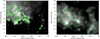 |
Fig. 1 Images of the Dragonflsh nebula covering the region studied in this work. Left panel: mosaic obtained by assembling 27 Spitzer IRAC images in the 8 μm band. Right panel: map retrieved from the Planck Legacy Archive (HFI 545 GHz data). Both maps are in logarithmic greyscale. For reference, three contours have been drawn at 30, 60, and 100 MJy sr−1 (Spitzer map) and at 100, 150, and 200 MJy sr−1 (Planck map). |
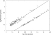 |
Fig. 2 Perimeter as a function of the area in pixels for objects (clouds) in the Dragonflsh nebula using the Spitzer (open circles) and Planck (open square) maps. Planck data have been vertically shifted by −0.5 for clarity. The solid lines are the corresponding best linear fits for all the data points. |
3 Young stellar object candidates
3.1 Candidate selection
Within the selected region, we used VizieR4 (Ochsenbein et al. 2000) to search for all existing sources in the AllWISE catalogue (Wright et al. 2010; Cutri et al. 2021). A total of 110 401 sources were retrieved, including their IDs, positions, and photometry in the W1 – W4 and JHK bands. Then, we applied the multicolour criteria scheme proposed by Koenig & Leisawitz (2014) to identify YSO candidates. This selection scheme is based on applying different cuts in colour and magnitude in the WISE+2MASS bands to remove contaminants (star-forming galaxies, active galactic nuclei, and asymptotic giant branch stars) and to select YSOs of Classes I and II, and transition disks. The application of these criteria to our sample yielded a total of 1082 YSOs, of which 139 belong to Class I, 627 to Class II, and 316 are transition disk sources. Table 2 (fully available at the CDS) presents a list of the selected YSOs, including their properties as derived in this work. An example colour-colour diagram is shown in Fig. 3. Of the selected sample, 323 sources were previously reported either as YSOs or YSO candidates by other authors (Lumsden et al. 2013; Marton et al. 2016; Kuhn et al. 2021; Rimoldini et al. 2023; Zhang et al. 2023). Table 2 also includes the references for these previously identified YSOs. The remaining YSOs are new candidates that are identified for the first time in this work.
3.2 Physical properties of the selected young stellar objects
3.2.1 Distances
Of the 1082 selected YSOs, 135 objects have counterparts in the Gaia DR3 catalogue and therefore have available parallaxes. For these sources, we estimated their distances D from their parallaxes, taking into account the global parallax offset of −0.017 mas reported by Lindegren et al. (2021). In general, the obtained values of D are distributed over a relatively wide range of values, which is due in part to uncertainties in the parallaxes (see Fig. 4). The most frequent value is found around D ≃ 4000 pc. For parallaxes with relatively smaller errors (purple histogram in Fig. 4), the distribution changes slightly, but the mode of the distribution always remains in the range 3000–5000 pc. The distance of D ~ 4 ± 1 kpc to the Dragonflsh complex is smaller than some previous estimates of ~ 10 – 12 kpc (de la Fuente et al. 2016; De Buizer et al. 2022), but it is consistent with the ~4–5 kpc reported by other authors (Moisés et al. 2011; Rate et al. 2020).
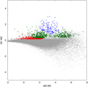 |
Fig. 3 Colour-colour diagram, W1 – W2 vs. W2 – W3, for all stars in the sample (grey dots) and for sources fulfilling criteria of Class I (blue dots), Class II (green dots), and transition disk (red dots) objects. |
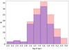 |
Fig. 4 Distribution of distances obtained from the parallaxes for the 135 stars with counterparts in Gaia DR3. The purple histogram refers to sources with a parallax error smaller than the parallax values themselves. |
3.2.2 Spectral energy distribution
The SEDs of the 1082 selected YSOs were analysed using the Virtual Observatory SED Analyzer (VOSA) developed by the Spanish Virtual Observatory (see details on the operation and limitations of VOSA in Bayo et al. 2008). The tool VOSA provides a friendly and flexible environment for finding the theoretical spectral model that best fits the observed photometric data. VOSA allows users to search and expand available photometry, choose from a list of models, and define parameter ranges to search for the best fit. For the fitting procedure, we first requested VOSA to expand the SEDs with all the photometry it could find. VOSA itself handles outlier rejection, and when different photometric values are found for the same filters, it calculates and uses an average value for the final SED. We then requested VOSA to fit the SEDs by minimising the reduced chi-square with the latest version of the BT-Settl models, which are based on the CIFIST photospheric solar abundances (Caffau et al. 2011). The effective temperature (Teff) was left as a free parameter in the fitting process, which in the BT-Settl models ranges from 1200 ≤ Teff ≤ 7000 K. VOSA fitted the points of the SED that were not flagged with possible infrared excess, which it assumed to be around the W1 band. The fitting process in VOSA is not very sensitive to some parameters such as metallicity and log g (Bayo et al. 2008). We made several tests by fixing or constraining these parameters around the expected values and also leaving them completely free, and in general, the resulting fits were not significantly affected. We finally left log g as a totally free parameter and fixed the metallicity to the solar value, whereas the visual extinction (AV) was allowed to vary in the range 0 ≤ AV ≤ 10 mag. For sources for which the fitting process did not converge on reasonable solutions, we also tried an independent fitting with the ATLAS9 Kurucz ODFNEW/NOVER models (Castelli et al. 1997). For these cases, the temperature was allowed to vary in the range 3500 ≤ Teff ≤ 50 000 K and the remaining parameters were set to the same conditions as employed for the BT-Settl fits. In any case, all 1082 SEDs and their fits were visually examined to verify the adequacy of the fits and solutions found by VOSA.
For a total of 399 sources (37%), the corresponding SED was well fitted with either BT-Settl models (89% of the sources) or Kurucz models (11%). The temperatures Teff and extinctions AV that provided the best fits are reported in Table 2, and a histogram with the distribution of Teff values is shown in Fig. 5. About 50% of the sources have photospheric temperatures in the range 3000 ≲ Teff ≲ 5000 K, although there is also a significant population of cool stars (late-M stars or brown dwarfs) with Teff ≲ 2000 K). An example SED for the first star belonging to this group in our Table 2 is shown in Fig. 6, which shows the fit performed by VOSA using a BT-Settl model and the expected infrared excess that is likely produced by circumstellar dust. We did not detect significant patterns or correlations of Teff or AV with the spatial distribution or with any other relevant physical variable. This population of cool stars is subject to ongoing investigation.
Identified YSOs in the Dragonfish region.
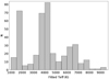 |
Fig. 5 Distribution of effective temperatures for the 399 sources whose SEDs could be fitted using VOSA (details in text). |
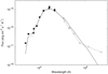 |
Fig. 6 Observed and best-fitted flux densities for one example source, J120022.63-631523.2, for which we obtained Teff = 1700 K and AV = 0.5, which is a transition disk object according to Koenig & Leisawitz (2014)’s criteria. The dashed line indicates the observed photometric data. Circles represent dereddened data, where solid circles denote data points that have been considered in the fitting process by VOSA. The solid lines indicate the best-fitted BT-Settl model. Some infrared excess is evident at wavelengths larger than ~10 μm. |
3.3 Spatial distribution
The spatial distribution of the selected YSOs, overlaid on the Spitzer map at 8 μm, is shown in Fig. 7. At first glance, younger classes (I and II) seem to follow the distribution of gas and dust exhibiting some level of clumpiness, whereas transition disk sources tend to be more homogeneously spread throughout the region. In order to objectively quantify the clumpiness, we used the so-called correlation dimension (Dc), which is suitable for analysing distributions of point sources. The correlation dimension measures the variation (as r increases) of the probability that two randomly chosen points are separated by a distance smaller than r (Grassberger & Procaccia 1983). For homogeneous point distributions in space, it is expected that Dc = 3, whereas in a plane, Dc = 2. When the points are distributed following fractal patterns, then Dc < 3 in the space or Dc < 2 in the plane. We used a previously developed and calibrated algorithm that estimated Dc in a precise and accurate manner (Sánchez et al. 2007a; Sánchez & Alfaro 2008). The algorithm constructs the minimum-area convex polygon to delimit the sample and avoid common problems at large scales (whole sample scale). On the other hand, at spatial scales of about the mean distance to the nearest neighbour, the distribution looks like a set of isolated points, and the obtained Dc values tend to zero (Smith 1988). Our algorithm uses suitable criteria to eliminate poorly estimated data (i.e. bad sampling) and thus to avoid these small-scale issues. Additionally, it applies bootstrapping techniques to estimate an uncertainty associated to Dc. The results from applying this algorithm are presented in Table 3. The estimation of the corresponding three-dimensional fractal dimension Df was made based on the simulations and results in Sánchez & Alfaro (2008).
The obtained Df values reveal a certain evolutionary process. Classes I and II exhibit approximately the same value of Df ≃ 1.7 ± 0.1. The slightly lower value of Dc (and Df) for the distribution of Class I objects is likely related to the relatively small number of sources (N = 139), because it has been shown that below N ~ 200 the retrieved value of Dc tends to be lower than the actual fractal dimension (see Fig. 2 in Sánchez & Alfaro 2008). In contrast, the more evolved transition disk objects show a significantly larger dimension with Df ≃ 2.2 ± 0.1. There is evidence for an evolutionary effect like this, where the initial hierarchical and clumpy structure gradually disappears over time (Elmegreen 2018). In external galaxies, the clumpy structure in the distribution of star formation sites has been observed to change towards smoother distributions as ages increase (Gieles et al. 2008; Sánchez & Alfaro 2008; Bastian et al. 2009; Bonatto & Bica 2010; Sánchez et al. 2010; Menon et al. 2021). At these scales (≳103 pc), the underlying cause may lie in non-turbulent motions acting at a galactic level, on scales of about or larger than the scale height of galactic disks (see discussions in Sánchez et al. 2010; Menon et al. 2021). In the case of star clusters, the observed initial substructures also seem to dissipate with age (Schmeja et al. 2008; Sánchez & Alfaro 2009; Ballone et al. 2020; Daffern-Powell & Parker 2020), but on these spatial scales (~10 pc), other physical processes may play important roles and the initial fractal structure is expected to be lost rapidly (Elmegreen 2018), either diluting into more homogeneous distributions in gravitationally unbound clusters or concentrating into radial density distributions in bound clusters. Nevertheless, the associated timescale is not clear, and some works suggested that cluster disruption may be a very slow process (≳10 Myr) in some cases (Hetem & Gregorio-Hetem 2019). In any case, different young clusters may reflect the initial structure of the different clouds from which they formed, and these conditions do not necessarily have to be the same. Therefore, the reported correlations between clumpiness and age for large samples of cluster could be contaminated by differences in initial conditions and might not correspond to any evolutionary effect. In the case of the Dragonfish complex, we focused on spatial scales of ~100 pc, where we detect a significant difference between the distributions of younger and more evolved stars, which marks an evolutionary effect. The underlying physical process is still not clear, but it may be related to the random stellar motion effect discussed by Elmegreen (2018), in which the initial clumpy structure disappears as stars age due to random turbulent velocity fields acquired at birth.
 |
Fig. 7 Spatial distribution of YSO candidates selected according to Koenig & Leisawitz (2014)’s criteria overlaid on the 8 μm band map from Spitzer IRAC. The green dots are sources that fulfil criteria of Class I (left panel), Class II (center panel), or transition disk (right panel) objects. |
Calculated fractal dimensions for the distribution of YSOs.
3.4 Hierarchy of structures
The previous analysis points out that YSOs are distributed in a clumpy manner and show some degree of substructure at different spatial scales. In this section, we address this issue by searching for density substructures in the YSO sample. To do this, we applied the algorithm OPTICS (Ordering Points To Identify the Clustering Structure; Ankerst et al. 1999) to perform a global analysis of the density structure of YSOs and retrieve a hierarchy of subclusters. OPTICS extends the clustering algorithm DBSCAN (Ester et al. 1996) to provide a global analysis of the density structure within a region and is especially well suited for samples with large density variations. DBSCAN groups points into clusters based on a density associated with two parameters: a minimum number of points Nmin, and a spatial scale ɛ. For each point, the scale ɛ defines a neighbourhood, and Nmin sets a density requirement for the neighbourhood. DBSCAN identifies clusters as composed of two types of points: Core points satisfy the density requirement, while border points belong to the ɛ-neighbourhood of a core point, but do not satisfy the density requirement themselves. The rest of the points are labelled as noise. In OPTICS, only the Nmin parameter is fixed and the concept of a reachability distance is introduced. We can intuitively interpret the reachability distance between a core point and another point as the minimum distance needed for the second point to be in the ɛ-neighbourhood of the core point, fulfilling the density threshold. OPTICS is not strictly a clustering algorithm, but an analytical tool whose main output is the reachability plot. The reachability plot shows the reachability distance of a reordered sample of points in a diagram where consecutive points are close and the clusters appear as dents or valleys. Based on the reachability plot, we can extract clusters either considering a height ɛ threshold (obtaining a clustering equivalent to DBSCAN with that ɛ) or with a slope ξ threshold (where clusters have a specific density ratio to their surroundings). We used the second approach because it can detect a hierarchy of structures that are nested within each other. We set a high value Nmin = 20 to limit the noise in the reachability plot and tested values of ξ ∈ [0.01, 0.1]. We finally chose ξ = 0.035 as a good compromise between the detection and reliability of the retrieved clusters.
Figures 8 and 9 show the reachability plot and a map with the convex hulls of the structures retrieved by OPTICS, in both cases labelled and colour-coded. In Table 4 we display the obtained characteristics of each structure. The whole sample is itself detected as a single structure by OPTICS, tagged and displayed in grey as structure 1 in Fig. 8, but not shown in Fig. 9 and Table 4 for the sake of clarity. The YSO sample exhibits a rich hierarchical structure, as expected from the previous fractal analysis. There are eight main structures, and structures 6 and 9 contain nested substructures. We assigned a level to each structure that was defined recursively by the number of substructures it contained: structures of level 0 do not contain any other, structures of level 1 contain structures of level 0, structures of level 2 contain structures of level 1, and so on. We find ten structures of level 0 (namely 2, 3, 4, 5, 6a, 6b, 7, 8, 9a1, and 9b), two of level 1 (6 and 9a), one of level 2 (9), and one of level 3 (structure 1, i.e. the whole sample). By considering a distance of ~4 kpc (see Sect. 3.2.1) and the average equivalent sizes of the structures for each level (shown in Table 4), we obtain that the spatial scales of the structures are about 15, 25, and 35 pc, which is typical of star-forming regions.
Table 4 also shows the correspondence between our detected structures and the star cluster candidates listed in Table 7 of de la Fuente et al. (2016). Fifteen of their 19 candidates are found within our structures. Our structure 3 includes the location of the H II region RCW 64 (Caswell & Haynes 1987) that de la Fuente et al. (2016) considered as a foreground region. However, four objects inside structure 3 have reliable parallaxes from Gaia DR3, which place this structure at a distance of ~3.8 ± 0.6 kpc. This is consistent with our estimate for the whole region (see Sect. 3.2.1). Structures 5, 6, and 9 contain three or more known star cluster candidates, and in the case of the most complex structure 9, its higher level substructure 9a1 contains five candidates and displays a clearly elongated shape. Even though environmental factors must play some role, the fraction of less evolved Class I sources to the total number of YSOs may yield some indications for the age of the structure (Evans et al. 2009). The variations in the spatial distribution of objects of different evolutionary stages have been used to investigate the star formation history within specific regions (see e.g. Sung et al. 2009; Venuti et al. 2018; Nony et al. 2021; Flaccomio et al. 2023) For the whole sample, the ratio of Class I/YSO is 12.9%, which is broadly consistent with the value 14.4% that we obtained when we considered only the clustered structures. However, we also identified structures with ratios higher than 20% and lower than 5%. Structures 2, 8 and 9a (in particular, 9a1) have significantly high Class I/YSO ratios that suggest a higher level of recent star formation, whereas structures 6a and 4 show significantly low ratios, pointing to areas where the star formation activity has declined. These results suggests a complex and varied star formation history in the Dragonfish complex, comprising different events spanning several million years.
List of retrieved clustered structures and substructures in the sample.
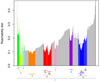 |
Fig. 8 Reachability plot obtained by OPTICS. The retrieved structures are colour-coded and labelled on the X-axis. |
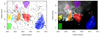 |
Fig. 9 Retrieved clustered structures and substructures in the sample. Left panel: YSOs (grey dots) and convex hulls of the structures, labelled and coloured as in Fig 8. The black asterisks are candidate or confirmed star clusters taken from Table 7 in de la Fuente et al. (2016). Right panel: overlap of the convex hulls of structures and the 8 μm emission map from Spitzer IRAC. |
4 Comparison of gas and young stellar object distributions
A primary goal of this work is to compare the distribution of gas and dust in the Dragonfish region with the distribution of young stars that were born from this gas. Because we used the same characterisation tool (the fractal dimension) for gas and for stars, we expect in principle to obtain nearly the same Df value for both components because at least in the case of ideal monofrac-tal clouds with dimension Df, the high-density peaks where star formation preferentially takes place are distributed following patterns with the same underlying dimension Df. In constrast, however, our results clearly indicate a scenario in which the distribution of younger objects is much more clumpy (Df ≃ 1.7) than the material from which they formed (Df ≃ 2.6 – 2.7).
Evidence supporting or contradicting either of these scenarios is far from being conclusive. The clustering strength of gas and newborn stars has not been studied in a direct, quantitative and self-consistent way so far. At spatial scales smaller than 500 pc, the galaxy M33 is more fragmented and irregular on average than the Milky Way, but its bright young stars are distributed following nearly the same fractal patterns as the molecular gas, both having Df ≲ 1.9 (Sánchez et al. 2010). In contrast, for the galaxy NGC 7793, Grasha et al. (2018) found that star clusters are distributed with a stronger clustering degree than giant molecular clouds over the range 40–800 pc on average; nevertheless, they also found approximately the same degree of clustering when they compared the most massive molecular clouds with the youngest and most massive star clusters. In any case, at spatial scales of about the disk scale height, the structure of the interstellar medium generated by turbulent motions may be somewhat affected by large-scale galactic dynamics, as discussed in Sánchez et al. (2010) and Menon et al. (2021). Gregorio-Hetem et al. (2015) calculated the clustering in a sample of young star clusters using the Q-parameter (Cartwright & Whitworth 2004) and also estimated the perimeter-area-based dimension Dper from visual extinction maps in the direction of these clusters. In general, they found that the substructures observed for the clusters were very similar to the fractal characteristics of the clouds, although an accurate comparison of the three-dimensional fractal dimension Df could not be made because projection effects were not properly taken into account. Parker & Dale (2015) performed a direct comparison of the spatial distributions of stars and gas in numerical simulations of molecular clouds using the Q-parameter for both stars and gas. Interestingly, they found that the formed stars followed a distribution that was highly substructured, with a value of Q ~ 0.4–0.7, which corresponds to approximately Df ~ 1.8–2.3 (see Fig. 7 in Sánchez & Alfaro 2009), whereas the gas from which stars formed had Q ~ 0.9, indicating a smooth, concentrated distribution of matter. These results should nevertheless be treated with some caution because, as indicated by Parker & Dale (2015), the Q-parameter may not be an optimal tool for measuring the spatial distribution of gas, since the pixelated image must previously be converted into a point distribution.
We found direct and self-consistent evidence that the clustering degree of newly born stars in the Dragonfish region is significantly higher than that of the parent cloud from which stars are forming. We mentioned that resolution issues (relatively large pixel sizes) could cause the gas maps to look smoother than they actually are, an effect that would not occur for the distribution of stars. However, this is likely not the cause of the observed difference between stars and gas because resolution effects and other factors (signal-to-noise ratio, cloud opacity) have already been calibrated and accounted for to accurately infer Df from Dper (Sánchez et al. 2005, 2007b). If this discrepancy is real, then there could be two possible explanations. On the one hand, the denser gas that is forming stars could be clumpier than the distribution of gas throughout the entire region, in concordance with a possible multifractal scenario, as proposed for the interstellar medium (Chappell & Scalo 2001). The approach used in this work aimed to avoid this issue by focusing on spatial scales of the same order for the cloud structure and the YSO distribution. On the other hand, the degree of clumpiness may somewhat increase during the star formation process. Although some simulations (e.g., Parker & Dale 2015) seem to support this possibility, the physical mechanisms driving this behaviour remain unclear. In simulations of fractal star clusters, Goodwin & Whitworth (2004) demonstrated that an initially homogeneous cluster can develop substructures if it is born with some coherence in the initial velocity field. It is not clear, however, whether this type of processes could operate at the spatial scale of a whole star-forming complex.
The relation between the spatial distributions of gas and formed stars remains as an intriguing and so far unresolved issue. The problem is non-trivial because the conversion from gas into stars, that is, the star formation process, involves many physical mechanisms that interact at different spatial scales. Moreover, the formation of stars does not occur synchronously throughout the entire cloud, and the first-formed stars can interact with the surrounding gas to modify its properties and also affect the distribution of subsequent stars.
5 Conclusions
We presented a systematic and detailed study of the Dragonfish star-forming region. On the one hand, we used different emission maps to characterise the distribution of gas and dust using fractal analysis. The three-dimensional fractal dimension obtained for the Dragonfish nebula was Df ≃ 2.6–2.7, a value that agrees very well with previously reported fractal dimensions for other molecular clouds, namely Orion, Ophiuchus, and Perseus. On the other hand, we used photometric information from the All-WISE catalogue to select and study a total of 1082 YSOs in this region. From the parallaxes measured by the Gaia mission for 135 of these sources, we derived a distance of D ~ 4 ± 1 kpc to the Dragonfish complex, and from the SED fitting to theoretical models, we also determined photospheric temperatures and visual extinctions for 399 sources. Regarding the spatial distribution of YSOs, we identified a clumpy a hierarchical assembly of structures and substructures, and moreover, we found that the clumpy structure of younger Class I and Class II sources tends to disappear for the more evolved sources (transition disks), suggesting some type of evolutionary effect. Interestingly, our fractal analysis clearly showed that the distribution of younger objects is much more clumpy (Df ≃ 1.7) than the distribution of the gas from which they formed (Df ≃ 2.6–2.7). Although some simulations (e.g., Parker & Dale 2015) seem to support the possibility that newly formed stars exhibit a more clumpy structure than their parent cloud, the physical mechanisms behind this behaviour remain unclear. In order to clarify this issue, it would be helpful to use strategies such as we proposed in this work, in which suitable and well-calibrated tools are used to simultaneously quantify the structure of both gas and stars in a relatively large sample of star-forming complexes.
Acknowledgement
We want to thank the referee for his/her helpful comments, which improved this paper. We acknowledge financial support from Univer-sidad Internacional de Valencia (VIU) through project VIU24003. The work of EN was supported by project VIU24007, funded by the reasearch center ESENCIA of VIU. J.B.C. was supported by projects PID2020-117404GB-C22, funded by MCIN/AEI, CIPROM/2022/64, funded by the Generalitat Valenciana, and by the Astrophysics and High Energy Physics programme by MCIN, with funding from European Union NextGenerationEU (PRTR-C17.I1) and the Generalitat Valenciana through grant ASFAE/2022/018. This research made use of Montage, that it is funded by the National Science Foundation under Grant Number ACI–1440620, and was previously funded by the National Aeronautics and Space Administration’s Earth Science Technology Office, Computation Technologies Project, under Cooperative Agreement Number NCC5–626 between NASA and the California Institute of Technology. We have made extensive use of VOSA, developed under the Spanish Virtual Observatory project funded by MCIN/AEI/10.13039/501100011033/through grant PID2020-112949GB-I00. We also have used the tool TOPCAT (Taylor 2005) and the NASA’s Astrophysics Data System.
Reference
- Allison, R. J., Goodwin, S. P., Parker, R. J., Portegies Zwart, S. F., & de Grijs, R. 2010, MNRAS, 407, 1098 [NASA ADS] [CrossRef] [Google Scholar]
- Ankerst, M., Breunig, M. M., Kriegel, H.-P., & Sander, J. 1999, SIGMOD Rec., 28, 49 [CrossRef] [Google Scholar]
- Arnold, B., Wright, N. J., & Parker, R. J. 2022, MNRAS, 515, 2266 [NASA ADS] [CrossRef] [Google Scholar]
- Ballone, A., Mapelli, M., Di Carlo, U. N., et al. 2020, MNRAS, 496, 49 [NASA ADS] [CrossRef] [Google Scholar]
- Bally, J. 2016, ARA&A, 54, 491 [Google Scholar]
- Bastian, N., Gieles, M., Ercolano, B., & Gutermuth, R. 2009, MNRAS, 392, 868 [NASA ADS] [CrossRef] [Google Scholar]
- Bates, M. L., & Whitworth, A. P. 2023, MNRAS, 523, 233 [NASA ADS] [CrossRef] [Google Scholar]
- Bates, M. L., Whitworth, A. P., & Lomax, O. D. 2020, MNRAS, 493, 161 [CrossRef] [Google Scholar]
- Bayo, A., Rodrigo, C., Barrado Y, Navascués, D., et al. 2008, A&A, 492, 277 [NASA ADS] [CrossRef] [EDP Sciences] [Google Scholar]
- Bazell, D., & Desert, F. X. 1988, ApJ, 333, 353 [NASA ADS] [CrossRef] [Google Scholar]
- Beattie, J. R., Federrath, C., & Klessen, R. S. 2019, MNRAS, 487, 2070 [NASA ADS] [CrossRef] [Google Scholar]
- Bergin, E. A., & Tafalla, M. 2007, ARA&A, 45, 339 [Google Scholar]
- Blaylock-Squibbs, G. A., Parker, R. J., Buckner, A. S. M., & Güdel, M. 2022, MNRAS, 510, 2864 [NASA ADS] [CrossRef] [Google Scholar]
- Bonatto, C., & Bica, E. 2010, MNRAS, 403, 996 [CrossRef] [Google Scholar]
- Buckner, A. S. M., Khorrami, Z., Khalaj, P., et al. 2019, A&A, 622, A184 [NASA ADS] [CrossRef] [EDP Sciences] [Google Scholar]
- Caffau, E., Ludwig, H. G., Steffen, M., Freytag, B., & Bonifacio, P. 2011, Sol. Phys., 268, 255 [Google Scholar]
- Cartwright, A., & Whitworth, A. P. 2004, MNRAS, 348, 589 [Google Scholar]
- Castelli, F., Gratton, R. G., & Kurucz, R. L. 1997, A&A, 318, 841 [NASA ADS] [Google Scholar]
- Caswell, J. L., & Haynes, R. F. 1987, A&A, 171, 261 [NASA ADS] [Google Scholar]
- Chappell, D., & Scalo, J. 2001, ApJ, 551, 712 [Google Scholar]
- Clarke, S. D., Jaffa, S. E., & Whitworth, A. P. 2022, MNRAS, 516, 2782 [NASA ADS] [CrossRef] [Google Scholar]
- Colombo, D., Rosolowsky, E., Ginsburg, A., Duarte-Cabral, A., & Hughes, A. 2015, MNRAS, 454, 2067 [NASA ADS] [CrossRef] [Google Scholar]
- Cutri, R. M., Wright, E. L., Conrow, T., et al. 2021, VizieR Online Data Catalog: II/328 [Google Scholar]
- Daffern-Powell, E. C., & Parker, R. J. 2020, MNRAS, 493, 4925 [Google Scholar]
- De Buizer, J. M., Lim, W., Karnath, N., Radomski, J. T., & Bonne, L. 2022, ApJ, 933, 60 [NASA ADS] [CrossRef] [Google Scholar]
- de la Fuente, D., Najarro, F., Borissova, J., et al. 2016, A&A, 589, A69 [NASA ADS] [CrossRef] [EDP Sciences] [Google Scholar]
- de La Fuente Marcos, R., & de La Fuente Marcos, C. 2006, A&A, 452, 163 [NASA ADS] [CrossRef] [EDP Sciences] [Google Scholar]
- Dib, S., Bontemps, S., Schneider, N., et al. 2020, A&A, 642, A177 [NASA ADS] [CrossRef] [EDP Sciences] [Google Scholar]
- Dickman, R. L., Horvath, M. A., & Margulis, M. 1990, ApJ, 365, 586 [CrossRef] [Google Scholar]
- Draine, B. T., & Li, A. 2007, ApJ, 657, 810 [CrossRef] [Google Scholar]
- Elia, D., Strafella, F., Schneider, N., et al. 2014, ApJ, 788, 3 [Google Scholar]
- Elia, D., Strafella, F., Dib, S., et al. 2018, MNRAS, 481, 509 [Google Scholar]
- Elmegreen, B. G. 2018, ApJ, 853, 88 [NASA ADS] [CrossRef] [Google Scholar]
- Elmegreen, B. G., & Elmegreen, D. M. 2001, AJ, 121, 1507 [CrossRef] [Google Scholar]
- Elmegreen, B. G., & Scalo, J. 2004, ARA&A, 42, 211 [Google Scholar]
- Ester, M., Kriegel, H.-P., Sander, J., & Xu, X. 1996, in Proceedings of the Second International Conference on Knowledge Discovery and Data Mining, KDD’96 (AAAI Press), 226 [Google Scholar]
- Evans, I., Neal, J., Dunham, M. M., Jørgensen, J. K., et al. 2009, ApJS, 181, 321 [NASA ADS] [CrossRef] [Google Scholar]
- Falgarone, E., Phillips, T. G., & Walker, C. K. 1991, ApJ, 378, 186 [NASA ADS] [CrossRef] [Google Scholar]
- Flaccomio, E., Micela, G., Peres, G., et al. 2023, A&A, 670, A37 [NASA ADS] [CrossRef] [EDP Sciences] [Google Scholar]
- Ghazzali, N., Joncas, G., & Jean, S. 1999, ApJ, 511, 242 [NASA ADS] [CrossRef] [Google Scholar]
- Gieles, M., Bastian, N., & Ercolano, B. 2008, MNRAS, 391, L93 [Google Scholar]
- Gomez, M., Hartmann, L., Kenyon, S. J., & Hewett, R. 1993, AJ, 105, 1927 [NASA ADS] [CrossRef] [Google Scholar]
- González, M., Joncour, I., Buckner, A. S. M., et al. 2021, A&A, 647, A14 [NASA ADS] [CrossRef] [EDP Sciences] [Google Scholar]
- Goodwin, S. P., & Whitworth, A. P. 2004, A&A, 413, 929 [NASA ADS] [CrossRef] [EDP Sciences] [Google Scholar]
- Grasha, K., Calzetti, D., Bittle, L., et al. 2018, MNRAS, 481, 1016 [NASA ADS] [CrossRef] [Google Scholar]
- Grassberger, P., & Procaccia, I. 1983, Phys. Rev. Lett., 50, 346 [NASA ADS] [CrossRef] [Google Scholar]
- Gregorio-Hetem, J., Hetem, A., Santos-Silva, T., & Fernandes, B. 2015, MNRAS, 448, 2504 [NASA ADS] [CrossRef] [Google Scholar]
- Hartmann, L. 2002, ApJ, 578, 914 [Google Scholar]
- Hetem, A., & Gregorio-Hetem, J. 2019, MNRAS, 490, 2521 [Google Scholar]
- Hetem, A. J., & Lepine, J. R. D. 1993, A&A, 270, 451 [NASA ADS] [Google Scholar]
- Houlahan, P., & Scalo, J. 1992, ApJ, 393, 172 [CrossRef] [Google Scholar]
- Jaffa, S. E., Whitworth, A. P., & Lomax, O. 2017, MNRAS, 466, 1082 [Google Scholar]
- Jaffa, S. E., Whitworth, A. P., Clarke, S. D., & Howard, A. D. P. 2018, MNRAS, 477, 1940 [NASA ADS] [CrossRef] [Google Scholar]
- Jaffa, S. E., Dale, J., Krause, M., & Clarke, S. D. 2022, MNRAS, 511, 2702 [NASA ADS] [CrossRef] [Google Scholar]
- Khalil, A., Joncas, G., & Nekka, F. 2004, ApJ, 601, 352 [NASA ADS] [CrossRef] [Google Scholar]
- Khalil, A., Joncas, G., Nekka, F., Kestener, P., & Arneodo, A. 2006, ApJS, 165, 512 [Google Scholar]
- Koenig, X. P., & Leisawitz, D. T. 2014, ApJ, 791, 131 [Google Scholar]
- Kraus, A. L., & Hillenbrand, L. A. 2008, ApJ, 686, L111 [Google Scholar]
- Kuhn, M. A., de Souza, R. S., Krone-Martins, A., et al. 2021, ApJS, 254, 33 [NASA ADS] [CrossRef] [Google Scholar]
- Larson, R. B. 1981, MNRAS, 194, 809 [Google Scholar]
- Larson, R. B. 1995, MNRAS, 272, 213 [NASA ADS] [Google Scholar]
- Lee, Y., Li, D., Kim, Y. S., et al. 2016, J. Korean Astron. Soc., 49, 255 [NASA ADS] [CrossRef] [Google Scholar]
- Lindegren, L., Bastian, U., Biermann, M., et al. 2021, A&A, 649, A4 [EDP Sciences] [Google Scholar]
- Lumsden, S. L., Hoare, M. G., Urquhart, J. S., et al. 2013, ApJS, 208, 11 [Google Scholar]
- Mandelbrot, B. B. 1983, The Fractal Geometry of Nature (New York: Freeman) [Google Scholar]
- Marchuk, A. A., Smirnov, A. A., Mosenkov, A. V., et al. 2021, MNRAS, 508, 5825 [NASA ADS] [CrossRef] [Google Scholar]
- Marton, G., Tóth, L. V., Paladini, R., et al. 2016, MNRAS, 458, 3479 [Google Scholar]
- McKee, C. F., & Ostriker, E. C. 2007, ARA&A, 45, 565 [Google Scholar]
- Menon, S. H., Grasha, K., Elmegreen, B. G., et al. 2021, MNRAS, 507, 5542 [CrossRef] [Google Scholar]
- Moisés, A. P., Damineli, A., Figuerêdo, E., et al. 2011, MNRAS, 411, 705 [CrossRef] [Google Scholar]
- Nony, T., Robitaille, J. F., Motte, F., et al. 2021, A&A, 645, A94 [NASA ADS] [CrossRef] [EDP Sciences] [Google Scholar]
- Ochsenbein, F., Bauer, P., & Marcout, J. 2000, A&AS, 143, 23 [NASA ADS] [CrossRef] [EDP Sciences] [Google Scholar]
- Parker, R. J., & Dale, J. E. 2015, MNRAS, 451, 3664 [NASA ADS] [CrossRef] [Google Scholar]
- Planck Collaboration I. 2011, A&A, 536, A1 [NASA ADS] [CrossRef] [EDP Sciences] [Google Scholar]
- Planck Collaboration X. 2016, A&A, 594, A10 [NASA ADS] [CrossRef] [EDP Sciences] [Google Scholar]
- Rahman, M., Matzner, C., & Moon, D.-S. 2011a, ApJ, 728, L37 [CrossRef] [Google Scholar]
- Rahman, M., Moon, D.-S., & Matzner, C. D. 2011b, ApJ, 743, L28 [NASA ADS] [CrossRef] [Google Scholar]
- Rate, G., Crowther, P. A., & Parker, R. J. 2020, MNRAS, 495, 1209 [NASA ADS] [CrossRef] [Google Scholar]
- Rimoldini, L., Holl, B., Gavras, P., et al. 2023, A&A, 674, A14 [NASA ADS] [CrossRef] [EDP Sciences] [Google Scholar]
- Robitaille, J. F., Joncas, G., & Khalil, A. 2010, MNRAS, 405, 638 [Google Scholar]
- Rosolowsky, E. W., Pineda, J. E., Kauffmann, J., & Goodman, A. A. 2008, ApJ, 679, 1338 [Google Scholar]
- Russeil, D. 1997, A&A, 319, 788 [NASA ADS] [Google Scholar]
- Sánchez, N., & Alfaro, E. J. 2008, ApJS, 178, 1 [CrossRef] [Google Scholar]
- Sánchez, N., & Alfaro, E. J. 2009, ApJ, 696, 2086 [Google Scholar]
- Sánchez, N. M., & Parravano, A. 1999, ApJ, 510, 795 [CrossRef] [Google Scholar]
- Sánchez, N., Alfaro, E. J., & Pérez, E. 2005, ApJ, 625, 849 [CrossRef] [Google Scholar]
- Sánchez, N., Alfaro, E. J., Elias, F., Delgado, A. J., & Cabrera-Cano, J. 2007a, ApJ, 667, 213 [CrossRef] [Google Scholar]
- Sánchez, N., Alfaro, E. J., & Pérez, E. 2007b, ApJ, 656, 222 [CrossRef] [Google Scholar]
- Sánchez, N., Añez, N., Alfaro, E. J., & Crone Odekon, M. 2010, ApJ, 720, 541 [CrossRef] [Google Scholar]
- Schinnerer, E., Meidt, S. E., Pety, J., et al. 2013, ApJ, 779, 42 [Google Scholar]
- Schmeja, S., Kumar, M. S. N., & Ferreira, B. 2008, MNRAS, 389, 1209 [CrossRef] [Google Scholar]
- Silverman, B. W. 1986, Density Estimation for Statistics and Data Analysis (London: Chapman and Hall/CRC) [Google Scholar]
- Simon, M. 1997, ApJ, 482, L81 [NASA ADS] [CrossRef] [Google Scholar]
- Smith, L. A. 1988, Phys. Lett. A, 133, 283 [NASA ADS] [CrossRef] [Google Scholar]
- Smith, J. D., Dale, J. E., Jaffa, S. E., & Krause, M. G. H. 2022, MNRAS, 516, 4212 [NASA ADS] [CrossRef] [Google Scholar]
- Stutzki, J., Bensch, F., Heithausen, A., Ossenkopf, V., & Zielinsky, M. 1998, A&A, 336, 697 [NASA ADS] [Google Scholar]
- Sun, J., Gutermuth, R. A., Wang, H., Zhang, S., & Long, M. 2022, MNRAS, 516, 5258 [NASA ADS] [CrossRef] [Google Scholar]
- Sung, H., Stauffer, J. R., & Bessell, M. S. 2009, AJ, 138, 1116 [Google Scholar]
- Taylor, M. B. 2005, ASP Conf. Ser., 347, 29 [Google Scholar]
- Venuti, L., Prisinzano, L., Sacco, G. G., et al. 2018, A&A, 609, A10 [NASA ADS] [CrossRef] [EDP Sciences] [Google Scholar]
- Vogelaar, M. G. R., & Wakker, B. P. 1994, A&A, 291, 557 [NASA ADS] [Google Scholar]
- Werner, M. W., Roellig, T. L., Low, F. J., et al. 2004, ApJS, 154, 1 [NASA ADS] [CrossRef] [Google Scholar]
- Wright, E. L., Eisenhardt, P. R. M., Mainzer, A. K., et al. 2010, AJ, 140, 1868 [Google Scholar]
- Zhang, C., Zhang, G.-Y., Li, J.-Z., & Yuan, J.-H. 2023, ApJS, 264, 24 [NASA ADS] [CrossRef] [Google Scholar]
All Tables
All Figures
|
Fig. 1 Images of the Dragonflsh nebula covering the region studied in this work. Left panel: mosaic obtained by assembling 27 Spitzer IRAC images in the 8 μm band. Right panel: map retrieved from the Planck Legacy Archive (HFI 545 GHz data). Both maps are in logarithmic greyscale. For reference, three contours have been drawn at 30, 60, and 100 MJy sr−1 (Spitzer map) and at 100, 150, and 200 MJy sr−1 (Planck map). |
| In the text | |
|
Fig. 2 Perimeter as a function of the area in pixels for objects (clouds) in the Dragonflsh nebula using the Spitzer (open circles) and Planck (open square) maps. Planck data have been vertically shifted by −0.5 for clarity. The solid lines are the corresponding best linear fits for all the data points. |
| In the text | |
|
Fig. 3 Colour-colour diagram, W1 – W2 vs. W2 – W3, for all stars in the sample (grey dots) and for sources fulfilling criteria of Class I (blue dots), Class II (green dots), and transition disk (red dots) objects. |
| In the text | |
|
Fig. 4 Distribution of distances obtained from the parallaxes for the 135 stars with counterparts in Gaia DR3. The purple histogram refers to sources with a parallax error smaller than the parallax values themselves. |
| In the text | |
|
Fig. 5 Distribution of effective temperatures for the 399 sources whose SEDs could be fitted using VOSA (details in text). |
| In the text | |
|
Fig. 6 Observed and best-fitted flux densities for one example source, J120022.63-631523.2, for which we obtained Teff = 1700 K and AV = 0.5, which is a transition disk object according to Koenig & Leisawitz (2014)’s criteria. The dashed line indicates the observed photometric data. Circles represent dereddened data, where solid circles denote data points that have been considered in the fitting process by VOSA. The solid lines indicate the best-fitted BT-Settl model. Some infrared excess is evident at wavelengths larger than ~10 μm. |
| In the text | |
|
Fig. 7 Spatial distribution of YSO candidates selected according to Koenig & Leisawitz (2014)’s criteria overlaid on the 8 μm band map from Spitzer IRAC. The green dots are sources that fulfil criteria of Class I (left panel), Class II (center panel), or transition disk (right panel) objects. |
| In the text | |
|
Fig. 8 Reachability plot obtained by OPTICS. The retrieved structures are colour-coded and labelled on the X-axis. |
| In the text | |
|
Fig. 9 Retrieved clustered structures and substructures in the sample. Left panel: YSOs (grey dots) and convex hulls of the structures, labelled and coloured as in Fig 8. The black asterisks are candidate or confirmed star clusters taken from Table 7 in de la Fuente et al. (2016). Right panel: overlap of the convex hulls of structures and the 8 μm emission map from Spitzer IRAC. |
| In the text | |
Current usage metrics show cumulative count of Article Views (full-text article views including HTML views, PDF and ePub downloads, according to the available data) and Abstracts Views on Vision4Press platform.
Data correspond to usage on the plateform after 2015. The current usage metrics is available 48-96 hours after online publication and is updated daily on week days.
Initial download of the metrics may take a while.