| Issue |
A&A
Volume 683, March 2024
|
|
|---|---|---|
| Article Number | A3 | |
| Number of page(s) | 13 | |
| Section | Galactic structure, stellar clusters and populations | |
| DOI | https://doi.org/10.1051/0004-6361/202347937 | |
| Published online | 28 February 2024 | |
Co-moving groups around massive stars in the nuclear stellar disk
1
Instituto de Astrofísica de Andalucía (CSIC), University of Granada, Glorieta de la Astronomía s/n, 18008 Granada, Spain
e-mail: amartinez@iaa.es
2
European Southern Observatory, Karl-Schwarzschild-Strasse 2, 85748 Garching bei München, Germany
3
University of California, Los Angeles, Department of Astronomy, Los Angeles, CA 90095, USA
4
Centro de Astrobiología (CSIC/INTA), Ctra. de Ajalvir km. 4, 28850 Torrejón de Ardoz, Madrid, Spain
Received:
11
September
2023
Accepted:
28
November
2023
Context. Over the last ∼30 Myr, the nuclear stellar disk in the Galactic center has been the most prolific star-forming region of the Milky Way when averaged by volume. Remarkably, the combined mass of the only three clusters present today in the nuclear stellar disk adds up to only ∼10% of the total expected mass of young stars formed in this period. Several causes could explain this apparent absence of clusters and stellar associations. The stellar density in the area is so high that only the most massive clusters would be detectable against the dense background of stars. The extreme tidal forces reigning in the Galactic center could dissolve even the most massive of the clusters in just a few megayears. Close encounters with one of the massive molecular clouds, which are abundant in the nuclear stellar disk, can also rapidly make any massive cluster or stellar association dissolve beyond recognition. However, traces of some dissolving young clusters and associations could still be detectable as co-moving groups.
Aims. It is our aim to identify so far unknown clusters or groups of young stars in the Galactic center. We focus our search on known, spectroscopically identified massive young stars to see whether their presence can pinpoint such structures.
Methods. We created an algorithm to detect over-densities in the 5D space spanned by proper motions, positions on the plane of the sky, and line-of-sight distances, using reddening as a proxy for the distances. Since co-moving groups must be young in this environment, proper motions provide a good means to search for young stars in the Galactic center. As such, we combined publicly available data from three different surveys of the Galactic center, covering an area of ∼160 arcmin2 on the nuclear stellar disk.
Results. We find four co-moving groups around massive stars, two of which are very close in position and velocity to the Arches’ most likely orbit.
Conclusions. These co-moving groups are strong candidates to be clusters or associations of recently formed stars, showing that not all the apparently isolated massive stars are run-away former members of any of the three known clusters in the Galactic center or simply isolated massive stars. Our simulations show that these groups or clusters may dissolve beyond our limits of detection in less than ∼6 Myr.
Key words: proper motions / Galaxy: center / Galaxy: structure / infrared: general
© The Authors 2024
 Open Access article, published by EDP Sciences, under the terms of the Creative Commons Attribution License (https://creativecommons.org/licenses/by/4.0), which permits unrestricted use, distribution, and reproduction in any medium, provided the original work is properly cited.
This article is published in open access under the Subscribe to Open model. Subscribe to A&A to support open access publication.
1. Introduction
Located around the Galactic center (GC), 8.2 kpc away from Earth (GRAVITY Collaboration 2020), we find the nuclear stellar disk (NSD), a flat-rotating structure (Schonrich et al. 2015; Shahzamanian et al. 2022) of ∼200 pc across and ∼50 pc scale height (Launhardt et al. 2002; Gallego-Cano et al. 2020). The NSD is an old structure, with most of its stellar population at least ∼8 Gyr old (Nogueras-Lara et al. 2020).
The NSD constitutes an extreme environment marked by intense tidal forces, elevated stellar density, and exceptionally strong magnetic fields. Despite these challenging conditions, the NSD emits approximately 10% of the total Lyman continuum flux in the entire Milky Way, while occupying less than 1% of the galaxy’s volume (Morris & Serabyn 1996; Nishiyama et al. 2008; Launhardt et al. 2002). Recent studies suggest that intense star-forming activity occurred in the NSD between about 0.1 and 30 Myr ago, reaching a star-forming rate of about 0.1 M⊙ per year in this period (Matsunaga et al. 2011; Nogueras-Lara et al. 2020). This would correspond to more than 1 million solar masses of young stars. While such intensive star formation left clear signs in the form of massive stellar clusters and associations in the Milky Way’s disk, the evidence for recent star formation in the NSD is more indirect. For example, there are only two known massive young clusters, the Arches and Quintuplet clusters (both at projected distance of about 25 pc from Sagittarius A*), and one association of young, massive stars in the central parsec (Bartko et al. 2010; Lu et al. 2013). They formed between 2 and 6 Myr ago and are about 1 × 10⁴ M⊙ each. In addition, a few dozen massive young stars have been detected distributed throughout the central 100 pc (e.g., Dong et al. 2011; Cano-González et al. 2021; Clark et al. 2023). Finally, on the order of 1 × 10⁵ M⊙ of young stars of age ∼10 Myr have been reported in the SgrB1 HII region (Nogueras-Lara et al. 2022). Together, all these stars still make up only a fraction of the stars that formed in the past few tens of megayears, which begs the question of where the “missing” young stars are.
This absence of direct observations of the products of star formation is due to the peculiar characteristics of the GC region. On the one hand, the stellar surface density is extremely high, which makes it hard or even impossible to detect any but the most massive clusters in the form of local stellar over-densities.
On the other hand, extreme interstellar extinction and its variability on small angular scales means that young hot stars cannot be easily distinguished photometrically from cool, old giants (see Schoedel et al. 2014; Cano-González et al. 2021). The extreme and differential extinction in the GC (e.g., Nishiyama et al. 2009; Nogueras-Lara et al. 2019a) limits observations to the near-infrared wavelength range, where it is impossible to identify young clusters in color-magnitude diagrams (CMDs), which are highly affected by the reddening (Nogueras-Lara et al. 2018).
Also, strong tidal forces in the GC will dissolve a cluster as massive as the Arches in ≲10 Myr (Portegies Zwart et al. 2001; Kruijssen et al. 2014), blending it with the background population. Spectroscopy needs to be performed at high angular resolution, which implies a very small field of view. Therefore, conducting spectroscopic searches is not a practical option due to the extensive time required to sample the entire region. However some clusters and stellar associations could still be detectable as co-moving groups, which is a detection method that has hardly been explored so far (with the exception of Shahzamanian et al. 2019).
Several studies have shown how stellar kinematics can unveil different kinds of structures, such as open clusters in Gaia data (Castro-Ginard et al. 2018) or substructures in the Galactic plane of the Milky Way (Laporte et al. 2022). In the GC, stellar proper motions have previously been used to study the structure of the NSD (see for example Shahzamanian et al. 2022; Martínez-Arranz et al. 2022; Nogueras-Lara 2022). Membership probabilities and orbits for the Arches and Quintuplet clusters have also been derived using proper motion analysis (Hosek et al. 2022).
We have created a new method for revealing co-moving groups in the highly crowded environment of the GC. This tool is based on the Density-Based Spatial Clustering of Applications with Noise (DBSCAN) algorithm (Ester et al. 1996), and a similar version of it has previously been used by Castro-Ginard et al. (2018) to detect open clusters in Gaia Data Release 2 (DR2). In this case, we looked for over-densities in a 5D parameter space. In this paper we present four co-moving groups in the GC associated with four different massive stars (Fig. 1) identified by Dong et al. (2011).
 |
Fig. 1. Survey coverage, cluster orbits, and massive star distribution in the GC. Regions covered by Libralato et al. (2021; indicated by white boxes) are superimposed on a 4.5 μm Spitzer/IRAC image (Stolovy et al. 2006). The cyan and blue lines represent the most probable prograde orbits of the Arches and Quintuplet clusters, respectively, as determined by Hosek et al. (2022). The continuous line indicates movement toward the Galactic east (in front of the plane of the sky), while the dashed line indicates movement toward the Galactic west (behind the plane of the sky). The plotted points correspond to massive stars identified by Dong et al. (2011) for which proper motion data are available. Among these stars, the green points are associated with a co-moving group, and their ID numbers correspond to their index as listed in Libralato et al. (2021). The letters A and Q and the asterisk denote the positions of the Arches and Quintuplet clusters and SgrA*. |
2. Data
We used proper motion data from the catalog by Libralato et al. (2021, hereafter L21) acquired with the Hubble Space Telescope (HST) Wide-Field Camera 3 (WFC3), combined with photometric data from the GALACTICNUCLEUS catalog (Nogueras-Lara et al. 2018, 2019b) acquired with the Very Large Telescope’s High Acuity Wide-field K-band Imager (HAWKI) instrument. In order to test the cluster search algorithm we used proper motion catalogs for the Arches and the Quintuplet clusters by Hosek et al. (2022) and extinction maps and catalogs in the H and Ks band by Nogueras-Lara et al. (2021).
2.1. Proper motions
The catalog of L21 was produced based on two sets of observations covering the area inside the white boxes in Fig. 1. They were acquired with the near-infrared channel of the Wide-Field Camera 3, mounted on the HST, in October 2012 and August 2015. The proper motions were calibrated using reference stars for Gaia DR2 (Gaia Collaboration 2016). More details about the acquisition, reduction, and analysis of the data are available in L211. The final catalog consists of absolute proper motion measurements for ∼830 000 stars, which we trimmed in a similar way as done by Libralato et al. (2021), namely: we excluded stars with proper motions faster than 70 mas yr−1, we selected only stars with proper motion errors lower than the 85th percentile in bins of 0.1 mag width and, finally, we discarded stars with proper motion error bigger than 1 mas yr−1 (Fig. 2).
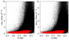 |
Fig. 2. Proper motion error versus magnitude in L21. Proper motion error in right ascension (left) and declination (right) versus F139M magnitude for the whole proper motion catalog (black) and the trimmed data (red). |
We cross-referenced the catalog with the GALACTICNUCLEUS survey (Nogueras-Lara et al. 2018, 2019b) to assign H and Ks magnitudes to the members of L21. GALACTICNUCLEUS was specifically designed to observe the GC, providing highly accurate point spread function photometry for over three million stars in the NSD and the innermost Galactic bar. The photometric uncertainties are remarkably low, remaining below 0.05 mag at H ∼ 19 mag and Ks ∼ 18 mag. Once we obtained H and Ks magnitude values for the L21 members, we employed a color cut H − Ks > 1.3 to remove the foreground population.
To assess the data quality, we extracted the mean velocity values for various components of the NSD and bulge from L21 and compared them with values reported in the literature. Further information about this process can be found in Appendix A.
3. Methods
We assumed that a stellar group would belong to the same cluster or stellar association if its members are close together in space and have similar velocities. It would be defined by a 6D parameter space, three dimensions for the components of the velocities and three for the components of the position. We only have data for proper motions and positions in the plane of the sky, but we can indirectly constrain the third dimension in position: the line-of-sight distance. Considering the considerable variation in extinction along the line of sight in the GC (e.g., Nishiyama et al. 2009; Nogueras-Lara et al. 2018), and the relatively constant intrinsic colors of the observable stars (they vary by not more than a few 0.01 mag; see for example Fig. 33 in Nogueras-Lara et al. 2018), we hypothesize that changes in color are mainly influenced by extinction (see also Nogueras-Lara et al. 2021). Therefore, if a group of stars shares similar colors, it is likely that they are located at a similar depth within the NSD (Nogueras-Lara 2022). We searched the data looking for over-densities in the 5D space formed by proper motions along the RA and Dec directions, coordinates in the plane of the sky, and color.
3.1. The algorithm
We developed a tool for detecting co-moving groups in the GC based on DBSCAN (Ester et al. 1996; Sander et al. 1998; Schubert et al. 2017). DBSCAN requires two input parameters: ϵ and Nmin. The parameter ϵ establishes the distance within which the algorithm scans for nearby points around a specific data point. Nmin specifies the minimum number of points that should be within the ϵ radius to form a dense region. Considering these two parameters DBSCAN classifies each point in one of these 3 categories: Core point, if the number of points around it within a radius of ϵ is ≥Nmin. Border Point, if it is not a core point, but it is within an ϵ distance of one, and Noise, if it is neither a core point nor a border point. The algorithm will iterate until all points are labeled with one of these categories. Core and border points are considered cluster members. As there is no preferred dimension in the 5D parameter space, we standardized the parameters. This means they have a mean of zero and a variance of one, ensuring that their contributions to the clustering process are balanced.
The conditions present in the NSD, where the stellar densities vary greatly on scales of a few arcseconds due to the high and patchy extinction (Nogueras-Lara et al. 2021) and the high densities of stars (Nogueras-Lara et al. 2019b), make the selection of ϵ particularly challenging. If we choose a value that is too small, the required minimum number of sources within a distance epsilon will never be fulfilled and no cluster will be found. On the other hand, if we choose a value that is too large, then spurious clusters present in the data just by chance will be detected because of statistical fluctuations.
In order to find an appropriate value for ϵ, we assumed that if there is a cluster in a particular dataset, then the distances among its members will be smaller, on average, than the distances between any other group of points in the same dataset. So, for each run of the algorithm we computed the distances to the kth nearest neighbor (k-NN) in the 5D space for all the stars in the area of analysis. Then, we generated a random sample with the same number of stars. To achieve this, we utilized the Gaussian kernel density estimator, specifically the gaussian_kde function from Scipy (Virtanen et al. 2020), to estimate the distribution of each astrometric parameter from the original dataset. We sampled from the estimated distributions to create a simulated population. Subsequently, we computed the k-NN distances for the simulated population. Since these populations are randomly generated, any existing clusters present in the original data are effectively destroyed in the simulated population. To mitigate the inherent variability resulting from the random generation of simulations, we performed 20 different simulations and calculated the average values. This approach allowed us to minimize the impact of slight differences between individual simulations.
If there were any cluster in the real data, then the minimum of the k-NN distances in the real data would be smaller than the minimum of the simulated data with no cluster in it. Next, we chose the value for ϵ as the mean between both minima, the real and the simulated one2. By choosing an epsilon smaller than the minimum neighbor distance for the simulated data, we tried to avoid any association of points that could show up in the data just by chance.
3.2. Testing the algorithm
To test our clustering tool, we used data from Hosek et al. (2022, H22 hereafter). They consist of astro-photometry data (equatorial coordinates, proper motions and magnitudes in F127M and F153M filters) acquired with the WFC3/HST camera in the areas of the Arches and Quintuplet clusters.
In H22, membership probabilities for the Arches and Quintuplet clusters are assigned, considering stars as cluster members if their membership probability is greater than 0.7. The membership probability assigned to each star by this work is based on the proper motions of the stars in an area of approximately 4 arcmin2 around each cluster. For further insight into the probability assignment process, refer to Appendix B in Hosek et al. (2022). Figure B.1 displays the stars identified as belonging to the Arches and Quintuplet clusters based on this criterion.
In the following, we describe the processes we undertook, using the data for the Arches cluster in H22 as an example. First, we chose a starting value. For this example we chose Nmin = 25. We tried our algorithm with different values of Nmin. We found that using any value of Nmin between 20 and 35 with H22 data returned similar values for proper motions and velocity dispersion as those found in H22 for both the Arches and Quintuplet datasets. Then we computed the 25-NN distance in a 5D space; velocity, position and color (black histogram in Fig. 3). Then we randomly generated a simulated population following the procedure described above, thus eliminating any real cluster from the data, and calculated the 25-NN distance for the simulated data (red histogram in Fig. 3). We can see that the real set of data, which we know has a cluster in it, has smaller minimum 25-NN distances than the set of simulated data with no real cluster in it. These lower values correspond to the points that are closest in the 5D space. Then we selected our ϵ as the mean value between the minimum of the real data and the minimum of the simulated data (green dashed line in Fig. 3).
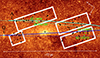 |
Fig. 3. NN distance analysis: Arches versus simulated data. The black histogram represents the distance of each point, in 5D space, to its 25-NN for the Arches data in H22. The red one is for the simulated data with no cluster. The green line marks the chosen value for epsilon in this particular case. |
Next we ran the algorithm on the Arches dataset of H22 with the ϵ and Nmin parameters that were set in the previous step. In Fig. 4 top row, we can see in orange the points labeled as cluster members that were returned by our algorithm. We repeated the process with the Quintuplet dataset (bottom row in Fig. 4). The mean values and their standard deviations for the proper motions that we obtain in each case are (μ∗RA,μDec)Arches = −0.85 ± 0.23, −1.89 ± 0.24 mas yr−1, and (μ∗RA,μDec)Quintuplet = −0.97 ± 0.19, −2.29 ± 0.22 mas yr−1 (left panels in Fig. 4). The values of the mean proper motions in both cases are similar to the ones obtained by Hosek et al. (2022): (μ∗RA,μDec)Arches H22 = −0.80, −1.89 mas yr−1, and (μ∗RA,μDec)Quintuplet H22 = −0.96, −2.29 mas yr−1. The velocity dispersions we obtained for both clusters, σ ∼ 0.2 mas yr−1, are comparable with the velocity dispersion found in other studies (Stolte et al. 2008, 2014; Clarkson et al. 2012). We computed the half-light radii of both clusters by transforming the magnitudes into fluxes using the Python package species (Stolker et al. 2020). These values are displayed in the orange boxes in the central plot of Fig. 4. The ratio between these radii, approximately 2, aligns with the values reported in the literature for the half-light radius of the Arches cluster (12.5 arcsec; Hosek et al. 2015) and the Quintuplet cluster (25 arcsec; Rui et al. 2019). The smaller half-light radii values we obtained may indicate the detection limit of our algorithm, which appears to be less sensitive to the outer members of the clusters. When comparing the stars identified as members of the Arches and Quintuplet clusters by our algorithm with those that H22 considered as likely members of the clusters (with membership probabilities p ≥ 0.7), we observe a level of completeness of approximately 42% for the Arches and approximately 31% for the Quintuplet. This represents approximately 45% of contamination in the Arches cluster and around 35% in the Quintuplet cluster found by our algorithm. These differences arise from restrictions in the parameter space of our algorithm. While the algorithm is configured to search for clusters in the 5D space, it also considers proximity in the parameter space defined by RA and Dec coordinates as a requirement for a star to be considered a cluster member. Consequently, stars farther away from the cluster core, which are likely members according to Hosek et al. (2022), are labeled as noise due to this criterion (see our Fig. B.1, top row). If we relax the restrictions of the algorithm and search only in the parametric space of velocities, the completeness level for the Arches and Quintuplet clusters with respect to those selected by H22 increases to 82% and 85%, respectively (Fig. B.1, bottom row). This represents 25% contamination in the Arches cluster and 15% for the Quintuplet found by the algorithm. However, it is important to note that due to the extreme crowding in the NSD and the fact that clusters as dense as the Arches or the Quintuplet are not expected to be found in the area, conducting a search for clusters or stellar associations using this configuration, which focuses solely on proximity in the velocity space, is not practical in the GC.
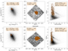 |
Fig. 4. Arches cluster (upper row) and Quintuplet cluster (lower row) as recovered by the algorithm in its 5D configuration. Left column: Vector-point diagram. Middle column: Stellar positions. Right column: CMD. Orange points represent the objects labeled as cluster members. Black points represent objects that are not labeled as cluster members. |
We compared the Arches catalog calculated by Clark et al. (2018a, hereafter C18) with the members identified in Hosek et al. (2022; see Fig. B.1 top row, left plots) and those selected by our algorithm using the 5D configuration (top row of Fig. 4). We display the matched positions in the top row of Fig. 5. The C18 catalog comprises 194 stars, including confirmed and candidate Arches members. The matches between H22 and C18 are approximately 50% of C18. In comparison, the percentage of matches with the algorithm-selected members is around 70% of C18. This may indicate that the algorithm in its 5D configuration is effective at identifying members at the core of the clusters. In the bottom row of Fig. 5, we present histograms of magnitude residuals for these matches. Given that the photometry in H22 and C18 originates from distinct catalogs, the low residual values with a mean of  , indicate non-spurious matches.
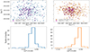 |
Fig. 5. Arches members: H22 versus 5D algorithm. Top row: Arches members according to H22 (blue points), those selected by the algorithm in the 5D configuration (orange points), and the matches with the Arches members considered in C18 for each case (fuchsia points). Bottom row: Magnitude residuals for the matches. |
The Arches cluster experiences a significant variation in extinction, as discussed in the study by Hosek et al. (2015). This is evident in the broader distribution observed in the CMD of the stars identified as Arches members (Fig. 4).
We ran a second test where we inserted the recovered Arches cluster, as determined by the algorithm in its 5D configuration, maintaining its original properties (see Fig. 4, top row) into a simulated population of stars. We then ran the cluster algorithm on this simulated population, which included the cluster. This simulated population consisted of the same objects as those in L21, but we shuffled the velocities of the stars while maintaining their positions. This velocity shuffling eliminated any possible substructure present in the catalog. Additionally, we excluded areas with the presence of dark clouds from the simulated population (see Fig. 3 in Nogueras-Lara et al. 2021). We first crossmatched the data from H22 with the GALACTICNUCLEUS catalog (Nogueras-Lara et al. 2018, 2019b) in order to assign H and Ks magnitudes to the stars, in the same way as we did with L21. Since the extinction is not homogeneous across the NSD, we had to correct the color of the cluster stars according to the value of extinction at the place where the stars will be inserted. For this purpose we used the extinction maps in H and Ks from Nogueras-Lara et al. (2021). We inserted and recovered the model cluster 50 times, placing it in random positions across the simulated population on each occasion. The first and second rows in Table 1 show the mean motions and their dispersions for the inserted and for the recovered clusters. The last two columns of the table show the percentage of recovered stars and the percentage of contaminating stars that the recovered cluster contained. We recovered on average more than 80% of the original stars with less than 20% of contamination from other stars. The difference in μ∗RA and μDec between inserted and recovered cluster is ∼2%.
Cluster recovering simulations.
Finally, in order to test the detection limit of the cluster algorithm, we repeated the experiment but this time we inserted less dense clusters. In order to simulate them, we used as models the recovered cluster parameters for Arches and Quintuplet from the H22 data (Fig. 4). Since the masses of both clusters are comparable, ∼104 M⊙ (Clarkson et al. 2012; Harfst et al. 2010) and they are in a similar environment, we assumed that they will evolve in a similar way. We used Quintuplet, with an age of ∼4 Myr (Figer et al. 1999; Liermann et al. 2012; Clark et al. 2018b) as a model for the evolutionary path that the younger Arches, ∼2.5 Myr (Figer et al. 1999; Najarro et al. 2004; Espinoza et al. 2009), would follow. By doing so, we could approximate the growth rate of the Arches cluster, assuming that its half-light radius will be similar to that of the Quintuplet in about 1.5 Myr. Next, we moved the Arches stars along the direction of their individual proper motion vectors, assuming this growth rate as constant over time. Then, we evolved the Arches cluster at different time lengths.
We inserted each of these models into the L21 data as we did before with the non-evolved models, and then ran our algorithm to recover them. This process was repeated 50 times for each model. The statistics for some of these simulations are presented in Table 1. Given that the environment changes with each insertion, the table displays the average and standard deviation for the 50 insertions. We defined the detection limit of our algorithm when the percentage of model stars recovered by the algorithm became lower than the percentage of contaminating stars in the recovered cluster (last two columns in Table 1). We can see that this limit is reached when our Arches model evolved ∼3.3 Myr. Based on this analysis, the detection of a hypothetical cluster as massive as the Arches, which has evolved over 6 Myr. since its formation, would exceed our detection limits: more than 50% of the members of this cluster would probably be contamination. This detection limit is comparable with theoretical predictions of the time it would take for a massive cluster to dissolve in the GC (Portegies Zwart et al. 2001; Kruijssen et al. 2014).
3.3. Mass estimation
In order to estimate the mass of the co-moving groups, we employed the Python package Spisea (Hosek et al. 2020). This package allows the generation of single-age, single-metallicity clusters, which we utilized to generate models for comparison with the selected co-moving groups. Firstly, we assigned extinction and differential extinction to the model. To compute these values, we utilized the extinction value of each star in the cluster from the catalog provided by Nogueras-Lara et al. (2021) along with its standard deviation. Secondly, we assigned a mass and an age to the model and generated a simulated cluster. Then, we established a reference interval using a bright and a faint star within our co-moving group. Next, we compared the number of stars within this interval in our simulated cluster to that of the co-moving group. If the simulated cluster had a higher number of stars within the interval, we adjusted the mass of the model to a smaller value and generated a new simulated cluster. We repeated this process, gradually decreasing the mass of our simulation by 1% increments until the number of stars in the reference interval of the model is not bigger than the number of stars inside the reference interval of the co-moving group.
To assess the reliability of this approach, we initially applied this procedure using the members considered likely to be part of the Arches cluster according to Hosek et al. (2022) (Fig. B.1, top row, left plots). The mean extinction was calculated by performing a crossmatch with the catalog for the GC by Nogueras-Lara et al. (2021). In addition, we assigned an age of 2.5 Myr to the model (Najarro et al. 2004; Espinoza et al. 2009) and solar metallicity (Najarro et al. 2004). We adopted a one-segment power-law model for the initial mass function (IMF) with a slope of α = −1.8, according to Hosek et al. (2019). Due to the quality of proper motion data in the catalog, for magnitudes fainter than K ∼ 17 and brighter than K ∼ 11, the number of stars generated in the simulated cluster differs significantly (by more than threefold) from the observed count in the Arches cluster. As a result, we limited the reference interval for comparison to stars with magnitudes between K = 17 and K = 11 mag. Then, we iteratively adjusted the model mass until the number of stars in the model was not greater than the number of stars in the cluster. The procedure was repeated 50 times, and the resulting mean mass and standard deviation values were recorded. We obtained an estimated mass of approximately 12 264 ± 495 M⊙, which is consistent with the estimated mass of the Arches cluster (Clarkson et al. 2012; Harfst et al. 2010). The results of one of these 50 runs are presented in Fig. 6.
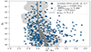 |
Fig. 6. Arches cluster versus simulated cluster: CMD comparison. The blue dots represent the members of the Arches cluster, while the gray dots represent a simulated cluster with an age of 2.5 Myr. The mean extinction is given by AKs = 1.85. The shaded area in the plot represents the uncertainty in the position of the model members in the CMD due to differential extinction, σAks. |
4. Results
Given the constraints posed by our algorithm and the relatively rapid dissolution of clusters in the NSD, we are compelled to confine our search to specific regions where the presence of young stars is likely. Thus, we restricted our search to around the massive stars listed in the catalog by Dong et al. (2011), which cannot be significantly older than 10 Myr. The maximum radius of the co-moving groups that we were able to recover from the simulation is ∼100 arcsec (∼4 pc). So, based on this, we limited the search area to a radius of 50 to 150 arcsec around the massive stars. Then, we identified the massive young stars from Dong et al. (2011) that have a counterpart in L21 after the quality cut. This selection accounts for a total of 59 objects, indicated by the black and green dots in Fig. 1.
We divided the search methodology into two distinct parts. Firstly, we applied our algorithm to each of the massive stars, exploring 20 different configurations. These configurations involved changes in the search radius (50, 75, 100, 125 n, and 150 arcsec) and the value for Nmin (15, 20, 25, and 30). In this initial phase, we identified and selected six distinct massive stars that exhibit co-movement within a group.
The high density of sources in the NSD increases the probability of stars being closely positioned in the 5D space, which could potentially lead to the detection of spurious clusters or associations. To address this issue, we conducted a simulation-based study as the second part of our analysis. In this phase, we ran our algorithm over simulated populations and compared the resultant clusters with those obtained from real data. We conducted this analysis for each of the previously identified co-moving groups, utilizing the stars in their vicinity as the basis for the simulated populations. In the simulations, we kept the positions and magnitudes of the sources unchanged while randomly mixing their velocities. We then applied the algorithm to the simulated population. Since the velocities of the stars were shuffled, any group found in the simulations would represent statistical clusters (i.e., the outcome of random associations). We repeated this process 10 000 times for each of the six cases. Subsequently, we compared the relationship between the area and the number of stars for these clusters with those found in the real data. The assigned area for each identified group corresponds to the minimum bounding box, calculated using the Python package alphashape. We show as an example the results of this analysis for the co-moving groups associated with the stars ID 14996 and 427662 (Figs. 7 and 8). We can see in the left plots of these figures that the area of the simulated clusters and the number of stars they contain exhibit a clear linear correlation. To quantitatively assess the likelihood that the co-moving group identified in the real data is merely a random association of stars, we compared it with the linear fit of the groups found in the simulations. Specifically, we compared the residual to the linear fit for the groups found in the simulations with the residuals to the same fit for the co-moving groups found in the real data. If the residuals of the co-moving group identified in the real data do not surpass the 3σ level of the residual distribution for the clusters found in the simulations, we discarded it. The right plots in Figs. 7 and 8 illustrate this comparison for the co-moving group associated with star ID 14996, which passed the cut, and ID 427662, which did not. We extended this analysis to all six identified co-moving groups linked to massive stars. Out of these, four groups successfully met the established criteria (green dots in Fig. 1) and were consequently considered unlikely to be the outcome of random stellar associations.
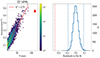 |
Fig. 7. Areal density of the co-moving group associated with star ID 14996 versus simulated clusters. Left: Area versus the number of stars for ∼15 000 statistical clusters identified by the algorithm across 10 000 simulated populations. The red line represents the linear fit between the area and the number of stars. The red triangle represents the co-moving group associated with star ID 14996. Right: Histogram showing the distribution of the residuals for the groups found in the simulated populations to the linear fit. The dashed blue lines mark the ±3σ levels of the distribution. The dashed red line marks the residual to the fit for the co-moving group associated with star ID 14996. |
Out of these four co-moving groups, the ones associated with the massive stars ID 14996 and 954199 significantly overlaps. Thus, we decided to run the algorithm around the barycenter of both massive stars. We found a single co-moving group containing both massive stars. Figure 9 shows the vector point diagram, positions and CMD for the co-moving group associated with star ID 14996 and ID 954199. Figure C.1 shows similar plots for the rest of the massive stars that are associated with a co-moving group that passed the final cut. In all three plots we show the co-moving groups with the smallest σμRA and σμDec that we found in each case. To provide a comparison, we have included red crosses to represent the stars surrounding the co-moving group within a distance of approximately 1.5 times the radius of the co-moving group. The corresponding values for these stars are displayed in the red boxes.
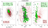 |
Fig. 9. Co-moving group analysis overview. From left to right: Vector-point diagram, coordinates, and CMD. Green points represent the members of the co-moving group. The blue circle and triangle represent the massive stars ID 14996 and ID 954199, respectively. Arrows indicate the direction in the equatorial reference frame. Inside the green boxes are the values for the mean proper motion and sigma for the co-moving group associated with star ID 14996, the number of stars members, the mean color and its sigma, and the maximum difference in color within the group. The radius represents half the distance between the two farthest members of the group. Red crosses mark the stars in the neighborhood of the co-moving group and black dots the rest of the stars in the area. |
The four massive stars associated with a co-moving group are classified by Dong et al. (2011) as either primary or secondary Paschen α emitters (Table 2), indicating that they are likely young stars. Furthermore, stars the with IDs 14996 and 154855 are reported by Clark et al. (2021) as a blue supergiant (O4-5 Ia+) and a Wolf-Rayet (WN8-9ha), respectively. This classification suggests that they cannot be older than a few million years.
Massive stars within a co-moving group.
The co-moving groups linked to stars ID 14996 and ID 954199 are associated with a known HII region (Dong et al. 2017), which further supports the presence of young stars. Both groups have a velocity comparable with the proper motions derived for the Arches cluster by Libralato et al. (2020) – μRA * = − 1.45 ± 0.23, μDec * = − 2.68 ± 0.14 mas yr−1 – which are also calibrated in Gaia DR2. Worth to mention that they lie along the path of the most probable orbit for the Arches cluster calculated by Hosek et al. (2022; cyan line in Fig. 1). The positions and velocities of these co-moving groups indicate that they may have formed in a similar location and possibly at a similar time as the Arches cluster. Another possibility is that these groups are part of the tidal tail resulting from the Arches cluster. The velocities and their projected distance from the Arches of approximately 20 pc align well with the tidal tail simulation presented in Habibi et al. (2014).
It is worth mentioning that a co-moving group of six stars in the same area was identified in a different study by Shahzamanian et al. (2019). This study used a different catalog and clustering method. Interestingly, three of these stars have a counterpart in the co-moving group associated with ID 14996. Additional investigations regarding this group will be presented in an upcoming publication (Martínez-Arranz et al., in prep.).
Regarding the groups associated with stars ID 154855 and 139573, they display similar velocities and comparable mean extinctions:  and
and  . Additionally, they are relatively close to each other in the plane of the sky. This proximity suggests that they may have been born as part of the same stellar formation process.
The mean color for all four co-moving groups is around  = 1.55 (Figs. 9 and C.1). This indicate that they are located close to the outer edge of the NSD (see Fig. 14 in Nogueras-Lara et al. 2019b).
Given the numerous unknown parameters involved, such as cluster membership probability, age, metallicity, and IMF, estimating the masses of the co-moving groups presented in Figs. 9 and C.1 becomes a challenging task. However, for the group associated with massive stars ID 14996 and 954199, if we consider the possibility that it formed through the same process that gave rise to the Arches cluster or is part of its tidal tail, we can adopt similar assumptions for their IMF, metallicity, and age as used for the mass estimation of the Arches cluster (Fig. 6). These assumptions include a top-heavy IMF (Hosek et al. 2019), a solar metallicity (Najarro et al. 2004) and an age of 2.5 Myr (Espinoza et al. 2009). Following a procedure similar to the one described in Sect. 3.3, we estimated the mass for this group (Fig. 10), and the results are presented in the first row of Table 2.
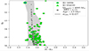 |
Fig. 10. Similar to Fig. 6 but for the co-moving group associated with star ID 14996. The point with a blue interior represents the massive star. |
For the groups associated with the massive stars ID 154855 and 139573, we conducted a series of simulations using various combinations of metallicity ([M/H] = 0 and [M/H] = 0.3), age (2, 5, and 8 Myr), and two different IMF models: the broken power-law derived by Kroupa (2001) and the top-heavy one derived by Hosek et al. (2019). This resulted in a total of 12 different combinations, each of which was run 50 times for both groups. The estimated masses, along with their standard deviations, are presented in Table 2.
All three groups exhibit velocity dispersions ranging from 0.72 to 0.83 mas yr−1. In our simulations (Table 1), the clusters with these values of velocity dispersion show a contamination level around 55 to 65%. Assuming a similar level of contamination in the co-moving groups we found, along with the aforementioned unknown parameters, could potentially result in variations in the estimated masses by a factor of approximately 2.
5. Discussion and conclusions
We have developed a method for scanning the GC for co-moving groups that offers the possibility of tackling the so-called missing cluster problem from a new angle. We present here the first results of this new analysis. We found four different co-moving groups around known massive stars in the NSD. Our toy model roughly estimates the time that it takes for a massive cluster in the GC to dissolve beyond the detection limit of our algorithm, and therefore we are able to restrict the age of the co-moving groups that we present. We believe that the presence of these groups constitutes direct evidence of recent star formation in the GC.
We analyzed the area around 59 known massive stars in the GC and find that four of them probably form part of a co-moving group. The relatively high velocity dispersion and low density of these co-moving groups, compared to those of the Arches or Quintuplet clusters, suggest two possible scenarios. Firstly, these co-moving groups may have originated from a dense cluster that has already undergone significant dissolution. Alternatively, they may have originated from a less dense stellar association. Recent studies have proposed that a substantial portion of the stars in the GC may have been born as part of loose associations of stars rather than gravitationally bound clusters (Ginsburg & Kruijssen 2018). Supporting this scenario, the identification of ∼105 M⊙ of young stars in the SgrB1 regions (Nogueras-Lara et al. 2022), which are only ∼5 Myr older than the Arches and Quintuplet clusters, provides further evidence. In the specific case of the group linked to the massive stars ID 14996 and 951499, there is a possibility that it is part of the tidal tail of the Arches cluster.
These groups show that not all apparently isolated massive stars in the NSD are run-away members from the nuclear star cluster, the Arches, or the Quintuplet. They highlight the location of stellar association and/or clusters smaller than Arches or Quintuplet and/or in an advanced state of dissolution (Dong et al. 2011).
On the one hand, the small number of co-moving groups detected by our analysis may be influenced by the quality of the dataset and by our conservative selection criteria. On the other hand, the large number of apparently unaccompanied massive young stars (along with the conclusion by L21 that they are not runaways from the known massive clusters) provides evidence that massive stars may form in isolation in the GC.
With the available datasets, we cannot estimate metallicities or radial velocities. Additionally, our estimations of ages and masses for the entire co-moving group are only rough approximations. To constrain these parameters and confirm the nature of these groups, future spectroscopy observations will be necessary.
The proper motions catalog that we used in this paper covers only a fraction of the NSD, and the uncertainty cut in proper motion that we made in the analysis significantly reduces the number of disposable sources. A wider and deeper set of data is necessary to continue with the search and corroborate these preliminary results. We are currently working on the reduction of a second epoch of GALACTICNUCLEUS that covers the NSD almost entirely. Combined with the first epoch (Nogueras-Lara et al. 2018), this will result in an unprecedented level of precision for proper motion measurements. Preliminary tests suggest an estimated uncertainty of ∼0.5 mas yr−1.
This new technique opens exciting possibilities for research of the GC. A more complete detection of young clusters in the NSD would allow us to address the crucial question of whether the IMF in the GC is fundamentally different from that in the Galactic disk.
A similar method for constraining the value of ϵ was used by Castro-Ginard et al. (2018).
Acknowledgments
Author Á. Martínez-Arranz and R. Schödel acknowledge financial support from the Severo Ochoa grant CEX2021-001131-S funded by MCIN/AEI/ 10.13039/501100011033 and support from the State Agency for Research of the Spanish MCIU through the “Center of Excellence Severo Ochoa” award for the Instituto de Astrofísica de Andalucía (SEV-2017-0709). Á. Martínez-Arranz and R. Schödel acknowledge support from grant EUR2022-134031 funded by MCIN/AEI/10.13039/501100011033 and by the European Union NextGenerationEU/PRTR and by grant PID2022-136640NB-C21 funded by MCIN/AEI 10.13039/501100011033 and by the European Union. We extend our gratitude to Paloma for generously sharing her expertise and guidance.
References
- Astropy Collaboration (Price-Whelan, A. M., et al.) 2022, ApJ, 935, 167 [NASA ADS] [CrossRef] [Google Scholar]
- Bartko, H., Martins, F., Trippe, S., et al. 2010, ApJ, 708, 834 [Google Scholar]
- Cano-González, M., Schödel, R., & Nogueras-Lara, F. 2021, A&A, 653, A37 [NASA ADS] [CrossRef] [EDP Sciences] [Google Scholar]
- Castro-Ginard, A., Jordi, C., Luri, X., et al. 2018, A&A, 618, A59 [NASA ADS] [CrossRef] [EDP Sciences] [Google Scholar]
- Clark, J. S., Lohr, M. E., Najarro, F., Dong, H., & Martins, F. 2018a, A&A, 617, A65 [NASA ADS] [CrossRef] [EDP Sciences] [Google Scholar]
- Clark, J. S., Lohr, M. E., Patrick, L. R., et al. 2018b, A&A, 618, A2 [NASA ADS] [CrossRef] [EDP Sciences] [Google Scholar]
- Clark, J. S., Patrick, L. R., Najarro, F., Evans, C. J., & Lohr, M. 2021, A&A, 649, A43 [NASA ADS] [CrossRef] [EDP Sciences] [Google Scholar]
- Clark, J. S., Lohr, M. E., Najarro, F., Patrick, L. R., & Ritchie, B. W. 2023, MNRAS, 521, 4473 [NASA ADS] [CrossRef] [Google Scholar]
- Clarkson, W. I., Ghez, A. M., Morris, M. R., et al. 2012, ApJ, 751, 132 [Google Scholar]
- Dong, H., Wang, Q. D., Cotera, A., et al. 2011, MNRAS, 417, 114 [Google Scholar]
- Dong, H., Lacy, J. H., Schödel, R., et al. 2017, MNRAS, 470, 561 [Google Scholar]
- Espinoza, P., Selman, F. J., & Melnick, J. 2009, A&A, 501, 563 [NASA ADS] [CrossRef] [EDP Sciences] [Google Scholar]
- Ester, M., Kriegel, H. P., Sander, J., & Xu, X. 1996, Proceedings of the Second International Conference on Knowledge Discovery and Data Mining, KDD’96 (AAAI Press), 226 [Google Scholar]
- Figer, D. F., Kim, S. S., Morris, M., et al. 1999, ApJ, 525, 750 [Google Scholar]
- Gaia Collaboration (Prusti, T., et al.) 2016, A&A, 595, A1 [NASA ADS] [CrossRef] [EDP Sciences] [Google Scholar]
- Gallego-Cano, E., Schödel, R., Nogueras-Lara, F., et al. 2020, A&A, 634, A71 [NASA ADS] [CrossRef] [EDP Sciences] [Google Scholar]
- Ginsburg, A., & Kruijssen, J. M. D. 2018, ApJ, 864, L17 [Google Scholar]
- Gordon, D., de Witt, A., & Jacobs, C. S. 2023, AJ, 165, 49 [NASA ADS] [CrossRef] [Google Scholar]
- GRAVITY Collaboration (Abuter, R., et al.) 2020, A&A, 636, L5 [NASA ADS] [CrossRef] [EDP Sciences] [Google Scholar]
- Habibi, M., Stolte, A., & Harfst, S. 2014, A&A, 566, A6 [NASA ADS] [CrossRef] [EDP Sciences] [Google Scholar]
- Harfst, S., Portegies Zwart, S., & Stolte, A. 2010, MNRAS, 409, 628 [NASA ADS] [CrossRef] [Google Scholar]
- Hosek, M. W., Jr., Lu, J. R., Anderson, J., et al. 2015, ApJ, 813, 27 [NASA ADS] [CrossRef] [Google Scholar]
- Hosek, M. W., Jr., Lu, J. R., Anderson, J., et al. 2019, ApJ, 870, 44 [NASA ADS] [CrossRef] [Google Scholar]
- Hosek, M. W., Jr., Lu, J. R., Lam, C. Y., et al. 2020, AJ, 160, 143 [NASA ADS] [CrossRef] [Google Scholar]
- Hosek, M. W., Do, T., Lu, J. R., et al. 2022, ApJ, 939, 68 [NASA ADS] [CrossRef] [Google Scholar]
- Kroupa, P. 2001, MNRAS, 322, 231 [NASA ADS] [CrossRef] [Google Scholar]
- Kruijssen, J. M. D., Longmore, S. N., Elmegreen, B. G., et al. 2014, MNRAS, 440, 3370 [Google Scholar]
- Kunder, A., Koch, A., Rich, R. M., et al. 2012, AJ, 143, 57 [NASA ADS] [CrossRef] [Google Scholar]
- Laporte, C. F. P., Koposov, S. E., & Belokurov, V. 2022, MNRAS, 510, L13 [Google Scholar]
- Launhardt, R., Zylka, R., & Mezger, P. G. 2002, A&A, 384, 112 [NASA ADS] [CrossRef] [EDP Sciences] [Google Scholar]
- Libralato, M., Fardal, M., Lennon, D., van der Marel, R. P., & Bellini, A. 2020, MNRAS, 497, 4733 [NASA ADS] [CrossRef] [Google Scholar]
- Libralato, M., Lennon, D. J., Bellini, A., et al. 2021, MNRAS, 500, 3213 [Google Scholar]
- Liermann, A., Hamann, W. R., & Oskinova, L. M. 2012, A&A, 540, A14 [NASA ADS] [CrossRef] [EDP Sciences] [Google Scholar]
- Lu, J. R., Do, T., Ghez, A. M., et al. 2013, ApJ, 764, 155 [NASA ADS] [CrossRef] [Google Scholar]
- Martínez-Arranz, Á., Schödel, R., Nogueras-Lara, F., & Shahzamanian, B. 2022, A&A, 660, L3 [NASA ADS] [CrossRef] [EDP Sciences] [Google Scholar]
- Matsunaga, N., Kawadu, T., Nishiyama, S., et al. 2011, Nature, 477, 188 [Google Scholar]
- Morris, M., & Serabyn, E. 1996, ARA&A, 34, 645 [Google Scholar]
- Najarro, F., Figer, D. F., Hillier, D. J., & Kudritzki, R. P. 2004, ApJ, 611, L105 [Google Scholar]
- Nishiyama, S., Nagata, T., Tamura, M., et al. 2008, ApJ, 680, 1174 [Google Scholar]
- Nishiyama, S., Tamura, M., Hatano, H., et al. 2009, ApJ, 696, 1407 [NASA ADS] [CrossRef] [Google Scholar]
- Nogueras-Lara, F. 2022, A&A, 668, L8 [NASA ADS] [CrossRef] [EDP Sciences] [Google Scholar]
- Nogueras-Lara, F., Gallego-Calvente, A. T., Dong, H., et al. 2018, A&A, 610, A83 [NASA ADS] [CrossRef] [EDP Sciences] [Google Scholar]
- Nogueras-Lara, F., Schödel, R., Najarro, F., et al. 2019a, A&A, 630, L3 [NASA ADS] [CrossRef] [EDP Sciences] [Google Scholar]
- Nogueras-Lara, F., Schödel, R., Gallego-Calvente, A. T., et al. 2019b, A&A, 631, A20 [NASA ADS] [CrossRef] [EDP Sciences] [Google Scholar]
- Nogueras-Lara, F., Schödel, R., Gallego-Calvente, A. T., et al. 2020, Nat. Astron., 4, 377 [Google Scholar]
- Nogueras-Lara, F., Schödel, R., & Neumayer, N. 2021, A&A, 653, A133 [NASA ADS] [CrossRef] [EDP Sciences] [Google Scholar]
- Nogueras-Lara, F., Schödel, R., & Neumayer, N. 2022, Nat. Astron., 6, 1178 [NASA ADS] [CrossRef] [Google Scholar]
- Portegies Zwart, S., Makino, J., McMillan, S., & Hut, P. 2001, ApJ, 565, 265 [Google Scholar]
- Rui, N. Z., Hosek, M. W., Jr., Lu, J. R., et al. 2019, ApJ, 877, 37 [NASA ADS] [CrossRef] [Google Scholar]
- Sander, J., Ester, M., Kriegel, H.-P., & Xu, X. 1998, Data Mining and Knowledge Discovery, 2, 169 [NASA ADS] [CrossRef] [Google Scholar]
- Schoedel, R., Feldmeier, A., Kunneriath, D., Stolovy, S., & Neumauer, N. 2014, VizieR Online Data Catalog: J/A+A/566/A47 [Google Scholar]
- Schonrich, R., Aumer, M., & Sale, S. E. 2015, ApJ, 812, L21 [NASA ADS] [CrossRef] [Google Scholar]
- Schubert, E., Sander, J., Ester, M., Kriegel, H. P., & Xu, X. 2017, ACM Trans. Database Syst., 42, 19 [CrossRef] [Google Scholar]
- Shahzamanian, B., Schödel, R., Nogueras-Lara, F., et al. 2019, A&A, 632, A116 [EDP Sciences] [Google Scholar]
- Shahzamanian, B., Schödel, R., Nogueras-Lara, F., et al. 2022, A&A, 662, A11 [NASA ADS] [CrossRef] [EDP Sciences] [Google Scholar]
- Sormani, M. C., Sanders, J. L., Fritz, T. K., et al. 2022, MNRAS, 512, 1857 [CrossRef] [Google Scholar]
- Speagle, J. S. 2020, MNRAS, 493, 3132 [Google Scholar]
- Stolker, T., Quanz, S. P., Todorov, K. O., et al. 2020, A&A, 635, A182 [EDP Sciences] [Google Scholar]
- Stolovy, S., Ramirez, S., Arendt, R. G., et al. 2006, J. Phys. Conf. Ser., 54, 176 [CrossRef] [Google Scholar]
- Stolte, A., Ghez, A. M., Morris, M., et al. 2008, ApJ, 675, 1278 [NASA ADS] [CrossRef] [Google Scholar]
- Stolte, A., Hußmann, B., Morris, M. R., et al. 2014, ApJ, 789, 115 [NASA ADS] [CrossRef] [Google Scholar]
- Virtanen, P., Gommers, R., Oliphant, T. E., et al. 2020, Nat. Meth., 17, 261 [Google Scholar]
Appendix A: Quality check
To assess the quality of the data, we identified the NSD and bulge through stellar kinematics and compared the obtained values with those reported in the literature. Firstly, we transformed the proper motions from equatorial to Galactic with the package SkyCoord from astropy (Astropy Collaboration 2022). Since the proper motions in the L21 catalog are in the Gaia DR2 reference frame, we further transformed them into a reference frame where SgrA* is at rest. This transformation involved subtracting the velocity of SgrA* in the International Celestial Reference Frame, which is (μl, μb)SgrA* = −6.40, −0.24 mas/yr (Gordon et al. 2023). In Fig. A.1 we can see the distribution of the Galactic proper motions of L21 for the components perpendicular and parallel to the Galactic plane (gray histograms). Then, we fit different Gaussian models to these distributions using the python package dynesty (Speagle 2020). We found that a two-Gaussians fit best reproduces the perpendicular component and three the parallel one (see Fig. A.1 and Fig. A.2). In Table A.1 we can see the values for these Gaussians, which we interpret as representative of the bulge and NSD populations (see Shahzamanian et al. 2022). In the left panel of Fig. A.1, the red Gaussian represents the bulge population and the black one the NSD. In the right panel, the red Gaussian also represents the bulge population. The blue one represents the stars of the NSD that stream toward the Galactic east and the black one those that stream toward the Galactic west. The bulge velocity in this reference frame should ideally be zero, but we can see that the parallel component is μl = 0.64 mas/yr. Due to data incompleteness, we tend to detect more stars from the near side of the NSD, introducing a bias in velocities toward stars moving to the west. To rectify this bias, we adjusted the bulge component to center it around zero. Consequently, the revised values for the NSD components are μl = 1.97 mas/yr and μl = -2.17 mas/yr. These revised results are consistent, within the known uncertainties, with the values previously determined for the mean velocities of stars in the NSD (Kunder et al. 2012; Schonrich et al. 2015; Shahzamanian et al. 2022; Sormani et al. 2022; Martínez-Arranz et al. 2022; Nogueras-Lara 2022). It is noteworthy to mention that in Libralato et al. (2021), the fitting of the data for the parallel component solely involves the use of two Gaussians, without considering the existence of the NSD.
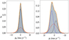 |
Fig. A.1. Proper motion distributions in L21. Gray histograms represent the proper motion distributions for the perpendicular (left) and parallel (right) proper motion components of the stars in L21. The red Gaussian represents the bulge stars in both plots. The black Gaussian on the left represents the perpendicular component of the NSD stars. On the right, the blue and black Gaussians represent stars on the near and far side of the NSD, respectively. |
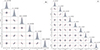 |
Fig. A.2. Posterior probability distributions of the free parameters for Gaussian fitting for the L21 proper motion distributions: the perpendicular component of the proper motions (left) and the parallel one (right). |
Best-fit parameters and uncertainties for L21 data (Fig. A.1).
Appendix B: Testing the algorithm
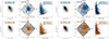 |
Fig. B.1. Comparison of Arches and Quintuplet clusters based on algorithm settings. In the top row, we present the members of the Arches and Quintuplet clusters according to Hosek et al. (2022). The blue points indicate stars with a likelihood ≥ 0.7 of belonging to the respective clusters, as determined in the aforementioned study. The red circles represent the half-light radii for each cluster, as found in the literature (Hosek et al. 2015; Rui et al. 2019). The left columns display the vector-point diagram, the middle columns show the stellar positions, and the right columns display the CMD. In the bottom row, we present the Arches and Quintuplet clusters as recovered by the algorithm when configured to search only in 2D space formed by the proper motion components. With this configuration, 75% of the stars labeled as Arches members match those of Hosek et al. (2022), and 85% in the case of Quintuplet cluster. |
Appendix C: Results
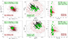 |
Fig. C.1. Same as Fig. 9 but for the rest of the massive stars that belong to a co-moving group (green points in Fig. 1). |
All Tables
All Figures
|
Fig. 1. Survey coverage, cluster orbits, and massive star distribution in the GC. Regions covered by Libralato et al. (2021; indicated by white boxes) are superimposed on a 4.5 μm Spitzer/IRAC image (Stolovy et al. 2006). The cyan and blue lines represent the most probable prograde orbits of the Arches and Quintuplet clusters, respectively, as determined by Hosek et al. (2022). The continuous line indicates movement toward the Galactic east (in front of the plane of the sky), while the dashed line indicates movement toward the Galactic west (behind the plane of the sky). The plotted points correspond to massive stars identified by Dong et al. (2011) for which proper motion data are available. Among these stars, the green points are associated with a co-moving group, and their ID numbers correspond to their index as listed in Libralato et al. (2021). The letters A and Q and the asterisk denote the positions of the Arches and Quintuplet clusters and SgrA*. |
| In the text | |
|
Fig. 2. Proper motion error versus magnitude in L21. Proper motion error in right ascension (left) and declination (right) versus F139M magnitude for the whole proper motion catalog (black) and the trimmed data (red). |
| In the text | |
|
Fig. 3. NN distance analysis: Arches versus simulated data. The black histogram represents the distance of each point, in 5D space, to its 25-NN for the Arches data in H22. The red one is for the simulated data with no cluster. The green line marks the chosen value for epsilon in this particular case. |
| In the text | |
|
Fig. 4. Arches cluster (upper row) and Quintuplet cluster (lower row) as recovered by the algorithm in its 5D configuration. Left column: Vector-point diagram. Middle column: Stellar positions. Right column: CMD. Orange points represent the objects labeled as cluster members. Black points represent objects that are not labeled as cluster members. |
| In the text | |
|
Fig. 5. Arches members: H22 versus 5D algorithm. Top row: Arches members according to H22 (blue points), those selected by the algorithm in the 5D configuration (orange points), and the matches with the Arches members considered in C18 for each case (fuchsia points). Bottom row: Magnitude residuals for the matches. |
| In the text | |
|
Fig. 6. Arches cluster versus simulated cluster: CMD comparison. The blue dots represent the members of the Arches cluster, while the gray dots represent a simulated cluster with an age of 2.5 Myr. The mean extinction is given by AKs = 1.85. The shaded area in the plot represents the uncertainty in the position of the model members in the CMD due to differential extinction, σAks. |
| In the text | |
|
Fig. 7. Areal density of the co-moving group associated with star ID 14996 versus simulated clusters. Left: Area versus the number of stars for ∼15 000 statistical clusters identified by the algorithm across 10 000 simulated populations. The red line represents the linear fit between the area and the number of stars. The red triangle represents the co-moving group associated with star ID 14996. Right: Histogram showing the distribution of the residuals for the groups found in the simulated populations to the linear fit. The dashed blue lines mark the ±3σ levels of the distribution. The dashed red line marks the residual to the fit for the co-moving group associated with star ID 14996. |
| In the text | |
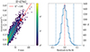 |
Fig. 8. Same as Fig. 7 but for the co-moving group associated with star ID 427662. |
| In the text | |
|
Fig. 9. Co-moving group analysis overview. From left to right: Vector-point diagram, coordinates, and CMD. Green points represent the members of the co-moving group. The blue circle and triangle represent the massive stars ID 14996 and ID 954199, respectively. Arrows indicate the direction in the equatorial reference frame. Inside the green boxes are the values for the mean proper motion and sigma for the co-moving group associated with star ID 14996, the number of stars members, the mean color and its sigma, and the maximum difference in color within the group. The radius represents half the distance between the two farthest members of the group. Red crosses mark the stars in the neighborhood of the co-moving group and black dots the rest of the stars in the area. |
| In the text | |
|
Fig. 10. Similar to Fig. 6 but for the co-moving group associated with star ID 14996. The point with a blue interior represents the massive star. |
| In the text | |
|
Fig. A.1. Proper motion distributions in L21. Gray histograms represent the proper motion distributions for the perpendicular (left) and parallel (right) proper motion components of the stars in L21. The red Gaussian represents the bulge stars in both plots. The black Gaussian on the left represents the perpendicular component of the NSD stars. On the right, the blue and black Gaussians represent stars on the near and far side of the NSD, respectively. |
| In the text | |
|
Fig. A.2. Posterior probability distributions of the free parameters for Gaussian fitting for the L21 proper motion distributions: the perpendicular component of the proper motions (left) and the parallel one (right). |
| In the text | |
|
Fig. B.1. Comparison of Arches and Quintuplet clusters based on algorithm settings. In the top row, we present the members of the Arches and Quintuplet clusters according to Hosek et al. (2022). The blue points indicate stars with a likelihood ≥ 0.7 of belonging to the respective clusters, as determined in the aforementioned study. The red circles represent the half-light radii for each cluster, as found in the literature (Hosek et al. 2015; Rui et al. 2019). The left columns display the vector-point diagram, the middle columns show the stellar positions, and the right columns display the CMD. In the bottom row, we present the Arches and Quintuplet clusters as recovered by the algorithm when configured to search only in 2D space formed by the proper motion components. With this configuration, 75% of the stars labeled as Arches members match those of Hosek et al. (2022), and 85% in the case of Quintuplet cluster. |
| In the text | |
|
Fig. C.1. Same as Fig. 9 but for the rest of the massive stars that belong to a co-moving group (green points in Fig. 1). |
| In the text | |
Current usage metrics show cumulative count of Article Views (full-text article views including HTML views, PDF and ePub downloads, according to the available data) and Abstracts Views on Vision4Press platform.
Data correspond to usage on the plateform after 2015. The current usage metrics is available 48-96 hours after online publication and is updated daily on week days.
Initial download of the metrics may take a while.