| Issue |
A&A
Volume 681, January 2024
|
|
|---|---|---|
| Article Number | L21 | |
| Number of page(s) | 6 | |
| Section | Letters to the Editor | |
| DOI | https://doi.org/10.1051/0004-6361/202348712 | |
| Published online | 23 January 2024 | |
Letter to the Editor
Hunting young stars in the Galactic centre
Hundreds of thousands of solar masses of young stars in the Sagittarius C region
European Southern Observatory, Karl-Schwarzschild-Strasse 2, 85748 Garching bei München, Germany
e-mail: This email address is being protected from spambots. You need JavaScript enabled to view it.
Received:
23
November
2023
Accepted:
29
December
2023
Abstract
Context. The Galactic centre stands out as the most prolific star-forming environment of the Galaxy when averaged over volume. In the last 30 million years, it has witnessed the formation of ∼106 M⊙ of stars. However, crowding and high extinction hamper their detection and, up to now, only a small fraction of the expected mass of young stars has been identified.
Aims. We aim to detect hidden young stars at the Galactic centre by analysing the stellar population in Sagittarius (Sgr) C. This is a region at the western edge of the nuclear stellar disc whose HII emission makes it a perfect candidate to host young stars.
Methods.We built dereddened luminosity functions for Sgr C and a control field in the central region of the nuclear stellar disc, and fitted them with a linear combination of theoretical models to analyse their stellar population.
Results. We find that Sgr C hosts several 105 M⊙ of young stars. We compared our results with the recently discovered young stellar population in Sgr B1, which is situated at the opposite edge of the nuclear stellar disc. We estimated that the Sgr C young stars are ∼20 Myr old, and likely show the next evolutionary step of the slightly younger stars in Sgr B1. Our findings contribute to addressing the discrepancy between the expected and the detected number of young stars in the Galactic centre, and shed light on their evolution in this extreme environment. As a secondary result, we find an intermediate-age stellar population in Sgr C (∼50% of its stellar mass with an age of between 2 and 7 Gyr), which is not present in the innermost regions of the nuclear stellar disc (dominated by stars > 7 Gyr). This supports the existence of an age gradient and favours an inside-out formation of the nuclear stellar disc.
Key words: dust / extinction / HII regions / Galaxy: center / Galaxy: nucleus / Galaxy: structure / infrared: stars
© The Authors 2024
 Open Access article, published by EDP Sciences, under the terms of the Creative Commons Attribution License (https://creativecommons.org/licenses/by/4.0), which permits unrestricted use, distribution, and reproduction in any medium, provided the original work is properly cited.
This article is published in open access under the Subscribe to Open model. This email address is being protected from spambots. You need JavaScript enabled to view it. to support open access publication.
1. Introduction
At only ∼8 kpc from Earth, the centre of the Milky Way is the closest galaxy nucleus and the only one where we can resolve stars down to milliparsec scales. It is roughly outlined by the nuclear stellar disc (NSD), a flat stellar structure of ∼109 M⊙ (e.g. Launhardt et al. 2002) with a scale length of ∼100 pc and a scale height of ∼40 pc (e.g. Gallego-Cano et al. 2020; Sormani et al. 2022).
Despite occupying less than 1% of the volume of the Galactic disc, the NSD is responsible for up to 10% of the star forming activity of the entire Milky Way over the past ∼100 Myr (e.g. Mezger et al. 1996; Mauerhan et al. 2010; Matsunaga et al. 2011; Crocker et al. 2011; Nogueras-Lara et al. 2020a, 2022). The detection of three classical Cepheids (Matsunaga et al. 2011) and the analysis of luminosity functions (e.g. Nogueras-Lara et al. 2020a) revealed that on the order of ∼106 M⊙ of stars formed there in the last 30 Myr. Nevertheless, the known young clusters (Arches and Quintuplet) and the young stars in the region only account for a small fraction of the expected young stellar mass (e.g. Figer et al. 1999a,b; Clarkson et al. 2012; Clark et al. 2021). This stark difference is known as the ‘missing clusters problem’.
The missing clusters problem is mainly due to the high crowding and stellar density in this region, in combination with the rapid dissolution of even massive clusters in the extreme environment there (∼6 Myr, for further details see Kruijssen et al. 2014). Moreover, the extreme extinction mostly limits the analysis of the NSD stars in the near-infrared (NIR; e.g. Nishiyama et al. 2006, 2008; Fritz et al. 2011; Nogueras-Lara et al. 2018, 2020b; Sanders et al. 2022), hampering the photometric detection of young stars. On the other hand, a spectroscopic search for young stars is not possible given the extremely high number of sources. An alternative way of detecting young stellar associations involves analysing stellar proper motions in order to identify comoving groups with a probable common and recent origin (e.g. Shahzamanian et al. 2019; Martínez-Arranz et al. 2023).
The recent analysis of Sagittarius (Sgr) B1, an HII region located at the eastern edge of the NSD (e.g. Simpson et al. 2018), revealed the presence of ∼105 M⊙ of young stars, suggesting that a significant fraction of the missing young stellar mass might be concealed within similar regions (Nogueras-Lara et al. 2022). In this context, Sgr C emerges as a promising candidate to host a substantial number of young stars. Located at the western edge of the NSD (Fig. 1), Sgr C shares similarities with Sgr B1, including strong HII emission (e.g. Lang et al. 2010), ongoing star formation, and the presence of some known young stars (e.g. Liszt & Spiker 1995; Forster & Caswell 2000; Kendrew et al. 2013; Lu et al. 2019a,b; Hankins et al. 2020), and therefore represents a unique region to search for young stars and assess whether or not they follow a symmetric distribution in the NSD, considering its position relative to Sgr B1.
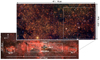 |
Fig. 1. Spitzer false-colour image using 3.6, 4.5, and 8 μm, as blue, green, and red, respectively (Stolovy et al. 2006). The white boxes indicate the position of Sgr C and Sgr B1, as well as the control field and the central NSD region. The black shaded area shows an avoided region in the analysis of the central NSD region in Nogueras-Lara et al. (2020a), corresponding to the nuclear star cluster. The small dashed rectangles indicate regions of particular interest within the Sgr C and Sgr B1 fields. The zoomed-in image corresponds to a GALACTICNUCLEUS JHKs false-colour image of the Sgr C field (see Sect. 4.1 for details). The white circles correspond to two WCL stars (Clark et al. 2021) and the dotted ellipse outlines a region where H2CO and CH3OH masers have been identified (Caswell 1996; Lu et al. 2019a). The compass indicates Galactic coordinates. |
In this Letter, we present a photometric analysis of the stellar population in a ∼8′×3.5′ field covering part of the Sgr C region. We analysed its dereddened Ks luminosity function and find that Sgr C contains several 105 M⊙ of young stars, which probably belong to young dissolved clusters and stellar associations. To best of our knowledge, our analysis constitutes the first stellar population characterisation of a western region of the NSD, and reveals the presence of a significant mass of young stars there.
2. Data
We used HKs photometry from the GALACTICNUCLEUS survey (Nogueras-Lara et al. 2018, 2019). This is a high-angular resolution (∼0.2″) NIR catalogue specially designed to observe the NSD. The GALACTICNUCLEUS survey reaches 5σ detections at H, Ks ∼ 21 mag, and the statistical uncertainties are below 0.05 mag at H ∼ 19 mag and Ks ∼ 19 mag. We chose a field covering the Sgr C region (D19; see Table A3 in Nogueras-Lara et al. 2019), and also a control field observed under similar conditions at the central region of the NSD (F19; see Table A1 in Nogueras-Lara et al. 2019). Figure 1 indicates the positions of these two fields.
The GALACTICNUCLEUS survey suffers from saturation in Ks band for stars brighter than 11.5 mag. To avoid this problem, we replaced the photometry of saturated sources and included non-detected bright stars using the SIRIUS IRSF survey (e.g. Nagayama et al. 2003; Nishiyama et al. 2006), as explained in Nogueras-Lara et al. (2020a).
3. Stellar population analysis
To analyse the stellar population in Sgr C and the control field, we built de-reddened Ks luminosity functions and fitted them with a linear combination of theoretical models applying the methodology outlined in, for example, Nogueras-Lara et al. (2020a); Nogueras-Lara et al. (2022) and Schödel et al. (2023).
3.1. Colour–magnitude diagram
Figure 2 shows the colour–magnitude diagram Ks versus H − Ks for the Sgr C region and the control field. To remove the contamination from foreground stars belonging to the Galactic disc and bar, we applied a colour cut given the significantly different extinction of these components in comparison to the Galactic centre (e.g. Sormani et al. 2020; Nogueras-Lara et al. 2021a,b). We used red clump (RC) stars (red giants in their helium core-burning sequence; Girardi 2016), as a reference for the colour cut, because they appear as a clear over-density in the colour–magnitude diagram and indicate the colour at which Galactic centre stars dominate. We chose H − Ks ∼ 1.6 mag and H − Ks ∼ 1.3 mag for the Sgr C and the control field, respectively. The redder cut for the Sgr C region indicates that the extinction is larger for this field.
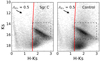 |
Fig. 2. Colour–magnitude diagram Ks versus H − Ks for the Sgr C field (left panel) and the control region (right panel). The red lines denote the colour cuts applied to remove foreground stars. The dashed rectangles show the red giant stars used to compute the extinction maps. The black arrows indicate the direction of the reddening vector. |
3.2. Extinction maps
To deredden the stars belonging to the Sgr C region and the control field, we created extinction maps following the methodology described in Nogueras-Lara et al. (2022). We defined a pixel size of ∼2″ and estimated the extinction using RC and red giant stars with similar intrinsic colours to a reference (see e.g. Nogueras-Lara et al. 2021b). We computed the extinction value (AKs) for each pixel by applying the equation:
 (1)
(1)
where AH/AKs = 1.84 ± 0.03 (Nogueras-Lara et al. 2020b), and the intrinsic colour of reference stars is (H − Ks)0 = 0.10 ± 0.01 mag (Nogueras-Lara et al. 2021b). We also applied an inverse distance weight method considering the five closest stars to a given pixel to account for the distance of the reference stars to each pixel. If fewer than five reference stars were present within a radius of ∼7.5″, we did not assign an extinction value for that particular pixel. Additionally, we required that the colour of the reference stars lie within 0.3 mag of the closest reference star to a given pixel. In this way, we accounted for potential extinction variation along the line of sight (e.g. Nogueras-Lara et al. 2020a, 2022). Figure 3 shows the obtained extinction map for Sgr C with a mean extinction of AKs = 2.56 ± 0.36 mag. Somewhat larger extinction values were measured for regions dominated by dust emission (inset in Fig. 3). A similar value was obtained for the control region with AKs = 2.26 ± 0.40 mag. The uncertainty refers to the standard deviation of the pixel values in each map.
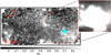 |
Fig. 3. AKs extinction map for Sgr C. The red dashed rectangle indicates a region of particular interest in Sgr C (see Sect. 4.1). The zoomed-in image shows a region of intense hot dust emission (24 microns, Carey et al. 2009). The cyan star and dashed circle indicate the centre and approximate extension of the HII region in the Sgr C complex (Lang et al. 2010), respectively. The compass corresponds to Galactic coordinates. |
3.3. Luminosity functions
We used the above extinction maps to correct the Ks photometry of both the Sgr C region and the control field. To prevent the inclusion of over-dereddened stars in the Ks luminosity function, we excluded stars whose dereddened H − Ks colour was more than 2σ bluer than the mean value of the dereddened distribution of the RC features (e.g. Nogueras-Lara et al. 2020a, 2022). We built the Ks luminosity function using the ‘auto’ option in the Python function numpy.histogram (Harris et al. 2020) to choose the bin width that maximises the Freedman–Diaconis (Freedman & Diaconis 1981) and Sturges (Sturges 1926) estimators. The associated uncertainty was calculated as the square root of the number of stars per magnitude bin.
Stellar crowding in the Galactic centre significantly reduces the number of stars in the faint end of the obtained luminosity functions (e.g. Nogueras-Lara et al. 2020a; Schödel et al. 2023). We therefore applied a completeness correction to account for this effect. We divided the Sgr C and the control fields into smaller subregions of ∼2′×2′ and calculated the completeness by estimating the critical distance at which a star is detectable in the vicinity of a brighter star, as explained in Eisenhauer et al. (1998) and Harayama et al. (2008). The final completeness solution for each field was computed by considering the mean and the standard deviation of the values obtained for each of the subregions. We applied the completeness solution to the Ks luminosity functions for each field, setting a lower limit of ∼90% of data completeness. This threshold corresponds to the value at which the Sgr C Ks luminosity function is limited by sensitivity (i.e. the number of stars in the luminosity function drastically drops beyond the adopted limit).
3.4. Fit of the Ks luminosity functions
To derive the stellar population in the Sgr C and the control regions, we fitted the Ks luminosity functions with a linear combination of theoretical models, as explained in Nogueras-Lara et al. (2020a); Nogueras-Lara et al. (2022) and Schödel et al. (2023). We used Parsec1 (Bressan et al. 2012; Chen et al. 2014, 2015; Tang et al. 2014; Marigo et al. 2017; Pastorelli et al. 2019, 2020) and MIST models (Paxton et al. 2013; Dotter 2016; Choi et al. 2016) with twice solar metallicity (e.g. Schultheis et al. 2019, 2021; Nogueras-Lara et al. 2020a, 2022), and similar stellar ages (14, 11, 8, 6, 3, 1.5, 0.6, 0.4, 0.2, 0.1, 0.04, 0.02, 0.01, and 0.005 Gyr). The ages of the models were chosen to account for the relevant changes in the shape of the Ks luminosity function with age, and also to specifically investigate the potential presence of the young stars with a good resolution (e.g. Nogueras-Lara et al. 2022).
We restricted the bright end of the luminosity function to Ks > 8 mag to avoid saturation problems that are also present in the SIRIUS IRSF data that we used to correct the GALACTICNUCLEUS photometry (see Sect. saturation and supplementary Fig. 4 in Nogueras-Lara et al. 2022). Given the lower extinction in the control field, we limited the bright end of its luminosity function to Ks = 8.5 mag, as done in previous work (Nogueras-Lara et al. 2022). We included a Gaussian smoothing factor to account for potential different distances between the stars (the NSD scale length is ∼100 pc; Gallego-Cano et al. 2020; Sormani et al. 2022) and some residual reddening, as well as a parameter to consider the distance towards the stellar populations.
Figure 4 shows the luminosity functions and the corresponding fits obtained by applying a χ2 minimisation when using Parsec models. To obtain the final results, we ran Monte Carlo simulations and created 1000 samples from the original luminosity function by randomly varying the number of stars per bin, assuming their corresponding uncertainty as the standard deviation of the distribution (Nogueras-Lara et al. 2022). We fitted each of the 1000 samples with the Parsec and MIST models and averaged over the results. We combined the models with similar ages into five age bins, merging models with similar ages to decrease the degeneracies (> 7, 2–7, 0.5–2, 0.06–0.5, and 0–0.06 Gyr). We obtained the contribution of each age bin to the stellar population by combining the results for Parsec and MIST models, quadratically propagating the corresponding uncertainties.
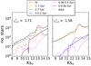 |
Fig. 4. Ks luminosity functions obtained for Sgr C (left panel) and the control field (right panel). The Parsec model fit and the reduced χ2 are indicated in each panel. Ks0 refers to the dereddened Ks magnitude. |
Figure 5 shows the results. We find the stellar populations in Sgr C and the control field to be significantly different. Sgr C shows a prominent contribution from young stars that is around six times larger than that of the control field. Moreover, approximately 50% of the total stellar mass in the Sgr C region is attributable to an intermediate-age stellar population (2–7 Gyr), which is not present in the control field (totally dominated by old stars).
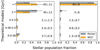 |
Fig. 5. Stellar populations in Sgr C (left panel) and the control field (right panel). The numbers in each panel indicate the percentage contribution of each age bin and its associated uncertainty. |
3.5. Total mass of young stars
We computed the total mass initially formed in the analysed Sgr C region using Parsec models that are calibrated in mass (e.g. Bressan et al. 2012; Chen et al. 2014, 2015; Tang et al. 2014; Marigo et al. 2017; Pastorelli et al. 2019, 2020). We adjusted the bin width of the Ks luminosity function to match that of the theoretical models and calculated the stellar mass by combining the contribution of each of the 14 models. We obtained a total stellar mass of (8.1 ± 0.9)×106 M⊙, where the values were estimated using the mean and the standard deviation of the mass distribution for the 1000 Monte Carlo samples. To estimate the total mass of young stars, we considered that 5.7 ± 0.9% of the total stellar mass was due to stars in the youngest age bin (5, 10, 20, 40 Myr, see Fig. 5). We obtain that (4.6 ± 0.1)×105 M⊙ of stars are younger than 60 Myr.
3.6. Systematic uncertainties
We assessed potential sources of systematic uncertainty on the analysis of the Sgr C luminosity function, without finding any significant variation with respect to the obtained results:
1. Initial mass function. Given that our sample consists almost entirely of giant stars, our results are almost completely insensitive to a change in the initial mass function (Schödel et al. 2023). We used a Salpeter function (Salpeter 1955) for the MIST models, and a Kroupa one (Kroupa et al. 2013) for the Parsec models. We made this different choice for the Parsec models because this is the only available initial mass function that also accounts for unresolved binaries. In any case, we also verified that using a Salpeter initial mass function for the Parsec models does not change our results in any significant way.
2. Bin width of the luminosity function. We repeated the analysis by assuming half and double the bin width previously estimated using the Python function numpy.histogram.
3. Bright end of the luminosity function. We assumed a bright end of the dereddened Ks luminosity function of 7.75 mag (0.25 mag brighter than the original one) and repeated the analysis.
4. Faint end of the luminosity function. We repeated the analysis considering different limits for the faint end. We assumed a completeness of ∼93% and ∼88%, which supposes a difference of ±0.4 mag in the faint end of the luminosity function.
5. Extinction map. We created a new extinction map, increasing the radius to search for reference stars to 10″ and choosing seven reference stars instead of five.
6. Metallicity of the stellar population. We repeated the analysis using Parsec models with solar metallicity.
4. Discussion
The high mass of young stars that we detect in Sgr C suggests the presence of a young stellar association that might have originally formed several stellar clusters (the upper mass limit for a young cluster in the Galactic centre is ∼104 M⊙; Trujillo-Gomez et al. 2019). The fact that there are no obvious stellar over-densities in Sgr C indicates that the young stellar population is already dispersed, which allows us to roughly estimate the age of the young stars to be ≳5 − 10 Myr, which corresponds to the time required to dissolve even massive clusters in the NSD (Portegies Zwart et al. 2002; Kruijssen et al. 2014).
Our analysis reveals that the Sgr C stellar population is similar to that in Sgr B1 (Nogueras-Lara et al. 2022). In both regions, there is an excess of young stars in comparison to the central area of the NSD. Additionally, they exhibit a similar contribution (∼40 − 50% of the total stellar mass) from an intermediate-age stellar population, with ages ranging from 2 to 7 Gyr. This is also significantly different from the stellar population in the central regions of the NSD, which is dominated by old stars (e.g. Nogueras-Lara et al. 2020a; Schödel et al. 2023), and indicates the presence of an age gradient with increasing stellar ages towards the centre of the NSD.
4.1. Young stars in a key Sgr C subregion
To better compare Sgr C and Sgr B1, we applied our luminosity function technique to a relatively small region of ∼50 pc2 (see Fig. 1), which likely contains an even higher fraction of young stars, as was done for a similar region in Sgr B (Nogueras-Lara et al. 2022). Figure 1 shows the chosen region, which includes the two known Wolf Rayet (WCL) stars in Sgr C (circles in Fig. 1; for further details see Clark et al. 2021), and several H2CO and CH3OH masers tracing recent star formation (Caswell 1996; Lu et al. 2019a). This area is also characterised by strong 24 micron emission (Carey et al. 2009), revealing the presence of hot dust likely associated to the HII region in Sgr C (see Fig. 3).
We find that the young stars (age bin < 60 Myr) in this region account for ∼7% of the total stellar mass, implying the presence of ∼1.5 × 10⁵ M⊙ of young stars. We also estimated the age of the stellar population by computing the contribution of the young models (5, 10, 20, 40 Myr) to each of the Monte Carlo samples. Figure 6 shows the obtained results. We find that the 20 Myr model is present in ≳98% of the 1000 Monte Carlo samples, and accounts for ∼5% of the total stellar mass when averaging over the results from Parsec and MIST models. This enables us to estimate that approximately 70% of the stellar mass attributed to young stars in this region is around 20 million years old.
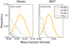 |
Fig. 6. Contribution of the young stellar models to the Ks luminosity function fit in the region dominated by hot dust emission in Sgr C (see Fig. 1). The solid line shows a Gaussian fit to the contribution of the 20 Myr model for Parsec (left panel) and MIST (right panel) models. The mean and the standard deviation of the Gaussian fits are indicated in each panel. |
Assuming a circular velocity for the NSD of ∼100 km s−1 (e.g. Schönrich et al. 2015; Sormani et al. 2022) and a distance of ∼70 pc for Sgr C from the supermassive black hole, we estimate the rotation period of the Sgr C stellar population to be ∼4 Myr. This implies that the detected young stellar population had enough time to complete several orbits around the NSD and did not form in situ. The presence of very young stars in the region, such as the H2CO and CH3OH masers (Caswell 1996; Lu et al. 2019a), could be due to ongoing star formation triggered by the outflows from the ionising stars of the detected ∼20 Myr stellar population. This mechanism might also explain the presence of the HII emission, in a similar way as proposed for the Sgr B1 region (e.g. Simpson et al. 2018). Moreover, Sgr C has been tentatively proposed as a connection point with one of the gas and dust streams linking the central molecular zone and the NSD to the Galactic bar (e.g. Molinari et al. 2011; Henshaw et al. 2023). This would explain the presence of a significant amount of dust, which is heated by the ionising stars, causing the intense 24 micron emission (Carey et al. 2009).
An analogous analysis carried out on a ∼40 pc2 region in Sgr B1 revealed the presence of a similar stellar mass of a slightly younger stellar population (∼5 − 10 Myr). Therefore, Sgr C likely represents the future state of the young stellar association in Sgr B1, and may provide crucial information for understanding the evolution of young stars in the Galactic centre and addressing the missing clusters problem.
4.2. Presence of an intermediate-age stellar population
A study of the external Milky Way-like galaxies from the TIMER survey (Gadotti et al. 2019) suggested that NSDs form inside-out from gas funnelled by galactic bars towards the innermost regions of the galaxies (Bittner et al. 2020). The recent analysis of the NSD stellar population along the line of sight revealed that the innermost region of the NSD is dominated by old stars, whereas the outer edge exhibits, on average, a younger stellar population (Nogueras-Lara et al. 2023). This finding supports the inside-out formation scenario and indicates that the NSD probably originated from gas funnelling towards the Galactic centre through the Galactic bar.
The study presented in this Letter, along with the results on the Sgr B1 region (Nogueras-Lara et al. 2022), allowed us to assess the inside-out formation growth of the NSD by analysing the stellar population at its centre (Nogueras-Lara et al. 2020a; Schödel et al. 2023) and its edges (Sgr B1 and Sgr C, see Fig. 1). Figure 7 shows our findings. While the central region of the NSD is dominated by an old stellar population (≳80% of the total stellar mass is older than ∼7 Gyr), Sgr C shows a stellar population akin to Sgr B1 (see Fig. 7). We find that ∼50% of its stellar mass falls within the age range of 2–7 Gyr. This supports the inside-out formation scenario and agrees with previous findings on the stellar population along the NSD line of sight (Nogueras-Lara et al. 2023).
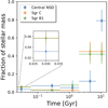 |
Fig. 7. Comparison between the stellar population present in the central region of the NSD, Sgr B1 (data extracted from Fig. 4 in Nogueras-Lara et al. 2022), and Sgr C (this work). The zoomed-in image shows the youngest age bin, where Sgr B1 and Sgr C show an excess of young stars in comparison to the central region of the NSD. |
Our results slightly disagree with the recent analysis of Mira variables in the NSD (Sanders et al. 2023), which only reveals weak evidence of inside-out growth. Nevertheless, these latter authors report a noteworthy population of Mira variables with periods of ∼400 days (equivalent to an age of ∼5 − 6 Gyr), which possibly correspond to stars accounting for the age gradient that we report here. Sanders et al. (2023) acknowledged that this stellar population was not distinctly identified in their modelling, which is possibly because of the smoothing applied to their spline model and the presence of particularly large uncertainties.
5. Conclusion
In this Letter, we present an analysis of the stellar population in Sgr C situated at the western edge of the NSD. Our findings reveal the presence of several 105 M⊙ of young stars, comprising ∼6% of the stellar mass in the region. This fraction is roughly six times larger than what we observed in a control field in the central region of the NSD, evidencing a clear excess of young stars. To best of our knowledge, our results constitute the first detection of a large population of young stars at the western edge of the NSD. This shows that the asymmetric gas distribution in the central molecular zone (e.g. Bally et al. 1988; Sormani et al. 2018) does not necessary imply an asymmetric distribution of young stars in the NSD.
Moreover, we compared the young stars in Sgr C with those in Sgr B1 located at the eastern edge of the NSD (Nogueras-Lara et al. 2022), and conclude that those in Sgr C are likely older. This implies that Sgr C may provide insights into the future evolution of the young stellar population in Sgr B1. In this way, it is now possible to identify regions that sample the various stages of young stellar evolution in the Galactic centre. Sgr B2 is a region of ongoing star formation (e.g. Ginsburg & Kruijssen 2018), the young Arches and Quintuplet clusters show a stellar population with ∼2–5 Myr (e.g. Najarro et al. 2004; Martins et al. 2008; Clark et al. 2018b,a), and finally Sgr B1 and Sgr C contain stellar associations with ∼10 and 20 Myr, respectively.
We also find that ∼50% of the total stellar mass in Sgr C is attributed to intermediate-age stars (∼2 − 7 Gyr). We compared our results with the central regions of the NSD and Sgr B1 and conclude that they support the presence of an age gradient in the NSD. Old stars dominate its central regions (e.g. Nogueras-Lara et al. 2020a; Schödel et al. 2023), while a younger stellar population (on average) appears close to the edge of the NSD (Nogueras-Lara et al. 2022, 2023). This points towards an inside-out formation of the NSD and suggests that bar-driven processes found in external barred galaxies are also at play in the Milky Way (Bittner et al. 2020).
Generated by CMD 3.6 (http://stev.oapd.inaf.it/cmd)
Acknowledgments
We thank the anonymous referee for helpful comments and suggestions that improved this manuscript. F.N.-L. gratefully acknowledges the sponsorship provided by the European Southern Observatory through a research fellowship. This work is based on observations made with ESO Telescopes at the La Silla Paranal Observatory under program ID195.B-0283. We thank the staff of ESO for their great efforts and helpfulness.
References
- Bally, J., Stark, A. A., Wilson, R. W., & Henkel, C. 1988, ApJ, 324, 223 [Google Scholar]
- Bittner, A., Sánchez-Blázquez, P., Gadotti, D. A., et al. 2020, A&A, 643, A65 [NASA ADS] [CrossRef] [EDP Sciences] [Google Scholar]
- Bressan, A., Marigo, P., Girardi, L., et al. 2012, MNRAS, 427, 127 [NASA ADS] [CrossRef] [Google Scholar]
- Carey, S. J., Noriega-Crespo, A., Mizuno, D. R., et al. 2009, PASP, 121, 76 [Google Scholar]
- Caswell, J. L. 1996, MNRAS, 283, 606 [NASA ADS] [CrossRef] [Google Scholar]
- Chen, Y., Girardi, L., Bressan, A., et al. 2014, MNRAS, 444, 2525 [Google Scholar]
- Chen, Y., Bressan, A., Girardi, L., et al. 2015, MNRAS, 452, 1068 [Google Scholar]
- Choi, J., Dotter, A., Conroy, C., et al. 2016, ApJ, 823, 102 [Google Scholar]
- Clark, J. S., Lohr, M. E., Najarro, F., Dong, H., & Martins, F. 2018a, A&A, 617, A65 [NASA ADS] [CrossRef] [EDP Sciences] [Google Scholar]
- Clark, J. S., Lohr, M. E., Patrick, L. R., et al. 2018b, A&A, 618, A2 [NASA ADS] [CrossRef] [EDP Sciences] [Google Scholar]
- Clark, J. S., Patrick, L. R., Najarro, F., Evans, C. J., & Lohr, M. 2021, A&A, 649, A43 [NASA ADS] [CrossRef] [EDP Sciences] [Google Scholar]
- Clarkson, W. I., Ghez, A. M., Morris, M. R., et al. 2012, ApJ, 751, 132 [Google Scholar]
- Crocker, R. M., Jones, D. I., Aharonian, F., et al. 2011, MNRAS, 413, 763 [NASA ADS] [CrossRef] [Google Scholar]
- Dotter, A. 2016, ApJS, 222, 8 [Google Scholar]
- Eisenhauer, F., Quirrenbach, A., Zinnecker, H., & Genzel, R. 1998, ApJ, 498, 278 [NASA ADS] [CrossRef] [Google Scholar]
- Figer, D. F., Kim, S. S., Morris, M., et al. 1999a, ApJ, 525, 750 [Google Scholar]
- Figer, D. F., McLean, I. S., & Morris, M. 1999b, ApJ, 514, 202 [Google Scholar]
- Forster, J. R., & Caswell, J. L. 2000, ApJ, 530, 371 [NASA ADS] [CrossRef] [Google Scholar]
- Freedman, D., & Diaconis, P. 1981, Probab. Theory Relat. Fields, 57, 453 [Google Scholar]
- Fritz, T. K., Gillessen, S., Dodds-Eden, K., et al. 2011, ApJ, 737, 73 [Google Scholar]
- Gadotti, D. A., Sánchez-Blázquez, P., Falcón-Barroso, J., et al. 2019, MNRAS, 482, 506 [Google Scholar]
- Gallego-Cano, E., Schödel, R., Nogueras-Lara, F., et al. 2020, A&A, 634, A71 [NASA ADS] [CrossRef] [EDP Sciences] [Google Scholar]
- Ginsburg, A., & Kruijssen, J. M. D. 2018, ApJ, 864, L17 [Google Scholar]
- Girardi, L. 2016, ARA&A, 54, 95 [Google Scholar]
- Hankins, M. J., Lau, R. M., Radomski, J. T., et al. 2020, ApJ, 894, 55 [NASA ADS] [CrossRef] [Google Scholar]
- Harayama, Y., Eisenhauer, F., & Martins, F. 2008, ApJ, 675, 1319 [Google Scholar]
- Harris, C. R., Millman, K. J., van der Walt, S. J., et al. 2020, Nature, 585, 357 [NASA ADS] [CrossRef] [Google Scholar]
- Henshaw, J. D., Barnes, A. T., Battersby, C., et al. 2023, ASP Conf. Ser., 534, 83 [NASA ADS] [Google Scholar]
- Kendrew, S., Ginsburg, A., Johnston, K., et al. 2013, ApJ, 775, L50 [NASA ADS] [CrossRef] [Google Scholar]
- Kroupa, P., Weidner, C., Pflamm-Altenburg, J., et al. 2013, Planets Stars Stellar Syst., 5, 115 [NASA ADS] [CrossRef] [Google Scholar]
- Kruijssen, J. M. D., Longmore, S. N., Elmegreen, B. G., et al. 2014, MNRAS, 440, 3370 [Google Scholar]
- Lang, C. C., Goss, W. M., Cyganowski, C., & Clubb, K. I. 2010, ApJS, 191, 275 [NASA ADS] [CrossRef] [Google Scholar]
- Launhardt, R., Zylka, R., & Mezger, P. G. 2002, A&A, 384, 112 [NASA ADS] [CrossRef] [EDP Sciences] [Google Scholar]
- Liszt, H. S., & Spiker, R. W. 1995, ApJS, 98, 259 [NASA ADS] [CrossRef] [Google Scholar]
- Lu, X., Mills, E. A. C., Ginsburg, A., et al. 2019a, ApJS, 244, 35 [Google Scholar]
- Lu, X., Zhang, Q., Kauffmann, J., et al. 2019b, ApJ, 872, 171 [Google Scholar]
- Marigo, P., Girardi, L., Bressan, A., et al. 2017, ApJ, 835, 77 [Google Scholar]
- Martínez-Arranz, Á., Schödel, R., Nogueras-Lara, F., Hosek, M., & Najarro, F. 2023, ArXiv eprints [arXiv:2309.06283] [Google Scholar]
- Martins, F., Hillier, D. J., Paumard, T., et al. 2008, A&A, 478, 219 [NASA ADS] [CrossRef] [EDP Sciences] [Google Scholar]
- Matsunaga, N., Kawadu, T., Nishiyama, S., et al. 2011, Nature, 477, 188 [Google Scholar]
- Mauerhan, J. C., Cotera, A., Dong, H., et al. 2010, ApJ, 725, 188 [Google Scholar]
- Mezger, P. G., Duschl, W. J., & Zylka, R. 1996, A&ARv, 7, 289 [NASA ADS] [CrossRef] [Google Scholar]
- Molinari, S., Bally, J., Noriega-Crespo, A., et al. 2011, ApJ, 735, L33 [Google Scholar]
- Nagayama, T., Nagashima, C., Nakajima, Y., et al. 2003, Proc. SPIE, 4841, 459 [NASA ADS] [CrossRef] [Google Scholar]
- Najarro, F., Figer, D. F., Hillier, D. J., & Kudritzki, R. P. 2004, ApJ, 611, L105 [Google Scholar]
- Nishiyama, S., Nagata, T., Kusakabe, N., et al. 2006, ApJ, 638, 839 [Google Scholar]
- Nishiyama, S., Nagata, T., Tamura, M., et al. 2008, ApJ, 680, 1174 [Google Scholar]
- Nogueras-Lara, F., Gallego-Calvente, A. T., Dong, H., et al. 2018, A&A, 610, A83 [NASA ADS] [CrossRef] [EDP Sciences] [Google Scholar]
- Nogueras-Lara, F., Schödel, R., Gallego-Calvente, A. T., et al. 2019, A&A, 631, A20 [NASA ADS] [CrossRef] [EDP Sciences] [Google Scholar]
- Nogueras-Lara, F., Schödel, R., Gallego-Calvente, A. T., et al. 2020a, Nat. Astron., 4, 377 [Google Scholar]
- Nogueras-Lara, F., Schödel, R., Neumayer, N., et al. 2020b, A&A, 641, A141 [EDP Sciences] [Google Scholar]
- Nogueras-Lara, F., Schödel, R., & Neumayer, N. 2021a, A&A, 653, A33 [NASA ADS] [CrossRef] [EDP Sciences] [Google Scholar]
- Nogueras-Lara, F., Schödel, R., & Neumayer, N. 2021b, A&A, 653, A133 [NASA ADS] [CrossRef] [EDP Sciences] [Google Scholar]
- Nogueras-Lara, F., Schödel, R., & Neumayer, N. 2022, Nat. Astron., 6, 1178 [NASA ADS] [CrossRef] [Google Scholar]
- Nogueras-Lara, F., Schultheis, M., Najarro, F., et al. 2023, A&A, 671, L10 [NASA ADS] [CrossRef] [EDP Sciences] [Google Scholar]
- Pastorelli, G., Marigo, P., Girardi, L., et al. 2019, MNRAS, 485, 5666 [Google Scholar]
- Pastorelli, G., Marigo, P., Girardi, L., et al. 2020, MNRAS, 498, 3283 [Google Scholar]
- Paxton, B., Cantiello, M., Arras, P., et al. 2013, ApJS, 208, 4 [Google Scholar]
- Portegies Zwart, S. F., Makino, J., McMillan, S. L. W., & Hut, P. 2002, ApJ, 565, 265 [NASA ADS] [CrossRef] [Google Scholar]
- Salpeter, E. E. 1955, ApJ, 121, 161 [Google Scholar]
- Sanders, J. L., Smith, L., González-Fernández, C., Lucas, P., & Minniti, D. 2022, MNRAS, 514, 2407 [CrossRef] [Google Scholar]
- Sanders, J. L., Kawata, D., Matsunaga, N., et al. 2023, MNRAS, submitted [arXiv:2311.00035] [Google Scholar]
- Schödel, R., Nogueras-Lara, F., Hosek, M., et al. 2023, A&A, 672, L8 [NASA ADS] [CrossRef] [EDP Sciences] [Google Scholar]
- Schönrich, R., Aumer, M., & Sale, S. E. 2015, ApJ, 812, L21 [Google Scholar]
- Schultheis, M., Rich, R. M., Origlia, L., et al. 2019, A&A, 627, A152 [NASA ADS] [CrossRef] [EDP Sciences] [Google Scholar]
- Schultheis, M., Fritz, T. K., Nandakumar, G., et al. 2021, A&A, 650, A191 [NASA ADS] [CrossRef] [EDP Sciences] [Google Scholar]
- Shahzamanian, B., Schödel, R., Nogueras-Lara, F., et al. 2019, A&A, 632, A116 [EDP Sciences] [Google Scholar]
- Simpson, J. P., Colgan, S. W. J., Cotera, A. S., Kaufman, M. J., & Stolovy, S. R. 2018, ApJ, 867, L13 [NASA ADS] [CrossRef] [Google Scholar]
- Sormani, M. C., Treß, R. G., Ridley, M., et al. 2018, MNRAS, 475, 2383 [NASA ADS] [CrossRef] [Google Scholar]
- Sormani, M. C., Magorrian, J., Nogueras-Lara, F., et al. 2020, MNRAS, 499, 7 [Google Scholar]
- Sormani, M. C., Sanders, J. L., Fritz, T. K., et al. 2022, MNRAS, 512, 1857 [CrossRef] [Google Scholar]
- Stolovy, S., Ramirez, S., Arendt, R. G., et al. 2006, J. Phys. Conf. Ser., 54, 176 [CrossRef] [Google Scholar]
- Sturges, H. A. 1926, J. Am. Stat. Assoc., 21, 65 [CrossRef] [Google Scholar]
- Tang, J., Bressan, A., Rosenfield, P., et al. 2014, MNRAS, 445, 4287 [NASA ADS] [CrossRef] [Google Scholar]
- Trujillo-Gomez, S., Reina-Campos, M., & Kruijssen, J. M. D. 2019, MNRAS, 488, 3972 [NASA ADS] [CrossRef] [Google Scholar]
All Figures
|
Fig. 1. Spitzer false-colour image using 3.6, 4.5, and 8 μm, as blue, green, and red, respectively (Stolovy et al. 2006). The white boxes indicate the position of Sgr C and Sgr B1, as well as the control field and the central NSD region. The black shaded area shows an avoided region in the analysis of the central NSD region in Nogueras-Lara et al. (2020a), corresponding to the nuclear star cluster. The small dashed rectangles indicate regions of particular interest within the Sgr C and Sgr B1 fields. The zoomed-in image corresponds to a GALACTICNUCLEUS JHKs false-colour image of the Sgr C field (see Sect. 4.1 for details). The white circles correspond to two WCL stars (Clark et al. 2021) and the dotted ellipse outlines a region where H2CO and CH3OH masers have been identified (Caswell 1996; Lu et al. 2019a). The compass indicates Galactic coordinates. |
| In the text | |
|
Fig. 2. Colour–magnitude diagram Ks versus H − Ks for the Sgr C field (left panel) and the control region (right panel). The red lines denote the colour cuts applied to remove foreground stars. The dashed rectangles show the red giant stars used to compute the extinction maps. The black arrows indicate the direction of the reddening vector. |
| In the text | |
|
Fig. 3. AKs extinction map for Sgr C. The red dashed rectangle indicates a region of particular interest in Sgr C (see Sect. 4.1). The zoomed-in image shows a region of intense hot dust emission (24 microns, Carey et al. 2009). The cyan star and dashed circle indicate the centre and approximate extension of the HII region in the Sgr C complex (Lang et al. 2010), respectively. The compass corresponds to Galactic coordinates. |
| In the text | |
|
Fig. 4. Ks luminosity functions obtained for Sgr C (left panel) and the control field (right panel). The Parsec model fit and the reduced χ2 are indicated in each panel. Ks0 refers to the dereddened Ks magnitude. |
| In the text | |
|
Fig. 5. Stellar populations in Sgr C (left panel) and the control field (right panel). The numbers in each panel indicate the percentage contribution of each age bin and its associated uncertainty. |
| In the text | |
|
Fig. 6. Contribution of the young stellar models to the Ks luminosity function fit in the region dominated by hot dust emission in Sgr C (see Fig. 1). The solid line shows a Gaussian fit to the contribution of the 20 Myr model for Parsec (left panel) and MIST (right panel) models. The mean and the standard deviation of the Gaussian fits are indicated in each panel. |
| In the text | |
|
Fig. 7. Comparison between the stellar population present in the central region of the NSD, Sgr B1 (data extracted from Fig. 4 in Nogueras-Lara et al. 2022), and Sgr C (this work). The zoomed-in image shows the youngest age bin, where Sgr B1 and Sgr C show an excess of young stars in comparison to the central region of the NSD. |
| In the text | |
Current usage metrics show cumulative count of Article Views (full-text article views including HTML views, PDF and ePub downloads, according to the available data) and Abstracts Views on Vision4Press platform.
Data correspond to usage on the plateform after 2015. The current usage metrics is available 48-96 hours after online publication and is updated daily on week days.
Initial download of the metrics may take a while.