| Issue |
A&A
Volume 696, April 2025
|
|
|---|---|---|
| Article Number | A213 | |
| Number of page(s) | 26 | |
| Section | Galactic structure, stellar clusters and populations | |
| DOI | https://doi.org/10.1051/0004-6361/202453414 | |
| Published online | 25 April 2025 | |
A spectroscopic map of the Galactic centre
Observations and resolved stars
1
Department of Astrophysics, University of Vienna,
Türkenschanzstrasse 17,
1180
Wien,
Austria
2
Max Planck Institute for Astronomy,
Königstuhl 17,
D-69117
Heidelberg,
Germany
3
Department of Physics and Astronomy, University of Utah,
Salt Lake City,
UT 84112,
USA
4
European Southern Observatory,
Karl-Schwarzschild-Strasse 2,
85748
Garching bei München,
Germany
5
ESA–ESAC–European Space Agency,
Camino Bajo del Castillo s/n,
28692
Villafranca del Castillo, Madrid,
Spain
6
European Space Research and Technology Centre,
Keplerlaan 1,
2200 AG
Noordwijk,
The Netherlands
7
Dipartimento di Fisica e Astronomia “Galileo Galilei”, Univ. di Padova, Vicolo dell’Osservatorio 3,
Padova
35122,
Italy
8
Technion – Israel Institute of Technology,
Haifa
3200002,
Israel
9
Instituto de Astrofísica de Andalucía (CSIC), Glorieta de la Astronomía s/n,
18008
Granada,
Spain
★ Corresponding author; This email address is being protected from spambots. You need JavaScript enabled to view it.
Received:
12
December
2024
Accepted:
10
March
2025
Abstract
Context. The Galactic centre (GC) region contains a dense accumulation of stars that can be separated into two components: a mildly flattened and extremely dense nuclear star cluster (NSC) and a surrounding more extended and more flattened nuclear stellar disc (NSD). Previous studies have collected a few thousand spectra of the inner NSC and the outer NSD and have measured line-of-sight velocities and metallicities. Until now, such measurements exist only for a few hundred stars in the region where the stellar surface density transitions from being dominated by the NSC to being dominated by the NSD.
Aims. We seek to study the stellar population from the centre of the NSC out to well beyond its effective radius, where the NSD dominates. In this way, we can investigate whether and how the mean properties and kinematics of the stars change systematically.
Methods. We conducted spectroscopic observations with Flamingos-2 in the K-band via a continuous slit scan. The data extend from the central NSC to the inner NSD, out to ±32 pc from Sgr A★ along Galactic longitude l. Based on their CO equivalent widths, we classified the stars in these areas as hot or cool stars. The former are massive young stars, while almost all of the latter are older than one to a few gigayears. Applying full-spectral fitting, we measured the overall metallicity [M/H] and line-of-sight velocity VLOS for more than 2500 cool stars, increasing existing samples outside of the very centre by a factor of three in terms of the number of stars and by more than an order of magnitude in terms of covered area. We present the first continuous spatial maps and profiles of the mean value of various stellar and kinematic parameters.
Results. We identify hot young stars across the field of view. Some stars appear to be isolated from other hot stars, while others accumulate within 2.7 pc of the Quintuplet cluster, or the central parsec cluster. The position-velocity curve of the cool stars shows no dependence on [M/H], but it depends on the colour of the stars. The colour may be a tracer of the line-of-sight distance and thus distinguish stars located in the NSC from those in the NSD. A subset of the cool stars has high velocities (i.e. greater than 150 km s−1), and they may be associated with the bar or tidal tails of star clusters.
Key words: stars: early-type / stars: late-type / Galaxy: center / Galaxy: kinematics and dynamics
© The Authors 2025
 Open Access article, published by EDP Sciences, under the terms of the Creative Commons Attribution License (https://creativecommons.org/licenses/by/4.0), which permits unrestricted use, distribution, and reproduction in any medium, provided the original work is properly cited.
This article is published in open access under the Subscribe to Open model. This email address is being protected from spambots. You need JavaScript enabled to view it. to support open access publication.
1 Introduction
The Galactic centre (GC) is an extremely dense environment with stellar densities several orders of magnitude higher than in the Galactic disc, a content of a few percent of the Milky Way’s molecular gas, and a star formation density that is more than two magnitudes higher than elsewhere in the Galaxy. These properties make the GC a region of special astrophysical interest. Because of extreme crowding and interstellar extinction, the GC is still far less explored by the great spectroscopic surveys than other parts of the Galaxy. Due to high extinction, stellar populations can only be studied in the infrared. However, their intrinsic stellar colour differences are significantly smaller than the extreme differential reddening that stars suffer in the line of sight to the GC, which impedes colour-magnitude diagram analyses. To study the stellar population in the GC, infrared spectroscopy is therefore required. Unfortunately, such data are sparse for the GC, as they are either targeted on individual bright stars (e.g. Fritz et al. 2021; Abdurro’uf et al. 2022) or concentrated in the inner parsec(s) (e.g. Feldmeier et al. 2014; Do et al. 2015; Fritz et al. 2016; von Fellenberg et al. 2022). Therefore, several pieces of the puzzle are missing to understand the formation and evolution of the inner part of the Milky Way.
The GC stellar content is sometimes referred to as the nuclear bulge, and it can be separated into two components: the more extended nuclear stellar disc (NSD) and the nuclear star cluster (NSC) within (Launhardt et al. 2002). The NSD appears as a thick disc that extends out to distances of r∼200 pc or more, with a radial scale length of ∼90 pc and a scale height of ∼28–45 pc (Launhardt et al. 2002; Nishiyama et al. 2013; Schödel et al. 2014; Gallego-Cano et al. 2020; Sormani et al. 2022). The flattening q (minor/major axis ratio) is ∼0.35, and the total mass derived from dynamical modelling is of the order of a few 108 to 109 M⊙ (Sormani et al. 2020, 2022). The NSC on the other hand is less flattened (q = 0.66–0.8) and smaller, with an effective radius of Re ∼5 pc (Launhardt et al. 2002; Schödel et al. 2014; Fritz et al. 2016; Gallego-Cano et al. 2020). Its total mass is of the order of a few 107 M⊙ (Feldmeier et al. 2014; Chatzopoulos et al. 2015; Fritz et al. 2016; Feldmeier-Krause et al. 2017b). Notably, the NSC contains the nearest supermassive black hole Sgr A★.
The stars in the innermost ∼1 pc region have been monitored over decades at the highest available spatial resolution (e.g. Do et al. 2009; Yelda et al. 2014; Habibi et al. 2017; von Fellenberg et al. 2022), resulting in a thorough knowledge of the stellar types and their three-dimensional kinematics. The more extended NSC and NSD are less well understood. Due to their large extent, observations are usually seeing limited and hence restricted to brighter stars compared to the innermost ∼1 pc (Feldmeier-Krause et al. 2017a; Nogueras-Lara et al. 2018; Feldmeier-Krause et al. 2020; Fritz et al. 2021; Feldmeier-Krause 2022).
Most stars in the GC are observed as red giant stars and are several gigayears old, though age estimates can differ by a few gigayears (Blum et al. 2003; Pfuhl et al. 2011; Schödel et al. 2020; Nogueras-Lara et al. 2020a; Chen et al. 2023). Hot young stars have also been discovered (e.g. O and B type main sequence, supergiant stars, Wolf Rayet stars, and emission line stars). These young massive stars appear to be separated into two groups. On the one hand, there are three massive (≳104 M⊙) clusters of young stars: the central parsec cluster, located in the very centre of the NSC, the Arches and the Quintuplet clusters, located on the east side of the NSD. Their stars are only a few megayears old (Figer et al. 1999; Najarro et al. 2004; Paumard et al. 2006; Liermann et al. 2012; Lu et al. 2013; Clark et al. 2018a,b). On the other hand, several dozens of apparently isolated young massive stars have been detected throughout the NSD (e.g. Cotera et al. 1999; Mauerhan et al. 2010b,a; Dong et al. 2011; Clark et al. 2021; Feldmeier-Krause 2022), and the census of hot stars in the GC is far from complete. There have been attempts to identify hot stars via their narrow-band photometry (Buchholz et al. 2009; Dong et al. 2011; Nishiyama & Schödel 2013; Plewa 2018; Nishiyama et al. 2023; Gallego-Cano et al. 2024). This method allows one to access larger areas and fainter stars at lower observational costs compared to spectroscopy. However, the hot star identification is less reliable, as lower mass intermediate-age stars can be mis-identified as hot young star candidates (Nishiyama et al. 2016), and hence spectroscopy is required to confirm the stellar type.
The several gigayears old red giant stars are the most numerous group of stars that are accessible for spectroscopy. Their metallicity distribution is broad, ranging from subto super-solar values, with a super-solar mean metallicity (Do et al. 2015; Rich et al. 2017; Feldmeier-Krause et al. 2017a, 2020; Thorsbro et al. 2020; Fritz et al. 2021; Feldmeier-Krause 2022). There is some evidence that the mean metallicity decreases from the inner NSC to the outer NSD and the bulge beyond (Schultheis et al. 2021; Feldmeier-Krause 2022; Nogueras-Lara et al. 2023a) and that the age decreases as a function of distance from Sgr A★ in the NSD (Nogueras-Lara et al. 2023b; Nogueras-Lara 2024). However, only limited data are available in the transition region, where the NSC stellar density drops to a value below the NSD and the NSD stars become dominant. Feldmeier-Krause (2022) present data of two fields located 20 pc away from Sgr A★. Still, there is no continuous spectroscopic coverage, and metallicity gradients and the velocity curve are based on fields located several parsecs apart. A continuous coverage of this region is of great interest to constrain the gravitational potential. There is also some debate about whether the NSC and the NSD are different entities or part of the same structure (Nogueras-Lara et al. 2023a).
In this study, we present what is so far the largest continuous spectroscopic data covering the NSC and the NSD out to 32 pc to the east and to the west of Sgr A★ along Galactic longitude, extending about 2 to 3 pc along Galactic latitude. We extract the spectra of the brightest stars, identify several hot stars, and measure the line-of-sight velocity VLOS and metallicity [M/H] of more than 2500 cool stars. We show the first continuous data on stellar metallicity and kinematics from the centre of the NSC across the transition region to the NSD and out to distances where the NSD dominates fully.
This paper is organised as follows. We present the data set, including data reduction, in Sect. 2, and we describe the analysis steps in Sect. 3. We present our hot star candidates in Sect. 4 and our red giant star kinematic and stellar population measurements in Sect. 5. We discuss our findings in Sect. 6 and conclude in Sect. 7.
 |
Fig. 1 Spatial coverage of our observations. The data extend ∼32 pc to the Galactic east and west of Sgr A★ (marked as a red plus symbol), about 1 pc to the Galactic north and south, except for the centre region, which extends about 2 pc to the Galactic north. The image is a white light reconstructed image mosaic of our spectroscopic scans. |
2 Spectroscopic data
2.1 Observations
We observed the GC on five nights (June 24, 25, 26, 27, 29, 2015) with Flamingos-2 (F2, Eikenberry et al. 2004), a nearinfrared imaging spectrograph at the Gemini South telescope. The observed five regions (Inner West, Outer West, Inner East, Outer East, and Centre) are centred on Sgr A★, and extend 32 pc to the Galactic east and 32 pc to the Galactic west; see also Fig. 1. We list further details on the observed regions in Table 1.
To cover a continuous region we resorted to long slit scans. Flamingos-2 is a multi-object spectrograph (MOS) that uses custom masks. Since the standard F2 long slit masks are only 4.′4 long, we designed a special mask that resembles a 6′ long slit. This was achieved by cutting six ≲1′ small slits or slitlets, aligned in a single row, with five small stabilising connectors that were not cut. Our slitlets are 1 pixel wide (0′′.18). The data were observed with the K-long filter (∼1.906–2.472 μm with 80% transmission) and R3K grism, with a maximum spectral resolution of R = 3400. We used the dark readout mode with 8 reads per exposure.
The observing strategy was as follows: for acquisition we usually took two images (6′ field-of-view), to be used for astrometric calibration. After inserting the slit mask with the slit aligned parallel to the Galactic plane, we took a series of five short (2 s) dark exposures to flush the detector and weaken the afterglow or persistence signal left from bright stars in the acquisition images. Then we started a series of usually 10 or 20 exposures of 300 s each, as listed in Table 1. The exact number of exposures per series varies from 6–22, as we sometimes had to stop a series early due to reaching zenith or approaching high airmass. Throughout the five nights, we observed 50 exposures per region, except for the central region, which extends further North, where we observed 87 exposures combined. During the observations, we drift-scanned the telescope slowly from Galactic north to Galactic south, with a rate of 1″ per 300 s, meaning each exposure covers a different ∼6′ × 1″ region of the sky. After an exposure series, that is four times per night, we made an offset to a dark sky field and took a series of four sky exposures. We observed early A-type dwarf stars as telluric standard stars (HD 171296, HD 175892) every two to three hours with the standard 1-pixel-wide long-slit mask and by offsetting along the slit with up to five exposures per star to account for the varying spectral resolution along the slit direction of the detector.
Flamingos-2 spectroscopic observations sorted by time.
2.2 Data reduction
The data were reduced with a combination of different tools. For basic reduction steps we used the GEMINI IRAF package, for telluric correction the ESO tool MOLECFIT, and for all remaining steps custom-made IDL and PYTHON scripts.
2.2.1 Basic reduction steps
We reduced the dark, flat, and arc exposures using IRAF and created Masterdarks, Masterflats, and wavelength solutions. The flats and arcs were cut into six pieces, one for each slitlet, as indicated by the MOS mask (using F2CUT). Also, the short and long wavelength ends, where the transmission is below ∼80%, were cut off. To create the Masterflat, we used NSFLAT, for the arc solution NSWAVELENGTH and a list of Argon lines in vacuum.
We applied dark subtraction on the object and sky data frames with the standard GEMARITH tool. Then we subtracted the persistence signal, which originates from the acquisition images, from the object spectral exposures, for details see Appendix A. Next, the data frames were cut along the slit direction using the MOS masks (F2CUT) into six pieces, and divided by the flat fields (NSREDUCE), which were cut in the same way. The four exposures of each sky series were combined into one Mastersky using the “crreject” algorithm in GEMCOMBINE, thus rejecting the brightest pixels of the set, which can be cosmic rays (CRs) or stars in the sky field. Next, we removed any remaining CRs or hot pixels with L.A. cosmic (van Dokkum 2001). We kept two versions of each file, one with CR rejection, and one without. The reason is that L.A. cosmic sometimes over-corrected bright stars. We used the uncorrected files for extracting bright stars, and the CR-corrected files for unresolved faint stars, which will be analysed in a separate paper (Feldmeier-Krause et al., in prep.). We rectified all files and applied the wavelength calibrations derived from the arc files (NSTRANSFORM). We also rectified the s-distortion, which we derived with NSSDIST from the many stars on the data themselves.
2.2.2 Sky line wavelength calibration correction
We took arc exposures each night, but in the course of a night, small wavelength shifts can occur. For this reason, we refined our wavelength calibration using the sky lines on our exposures and cross-correlating the spectra with a reference exposure.
As reference exposure, we chose the last exposure taken on the night of 2015-06-26, as it was taken closest in time to the arc exposure of that night. For each exposure and slitlet, we normalised the two-dimensional spectral frame by the median flux of each pixel row along the slit and then summed the flux to obtain a one-dimensional spectrum per exposure and slitlet that is dominated by the sky rather than bright stars. We then cross-correlated this sky-dominated spectrum with the reference sky-dominated spectrum in 14 wavelength regions ranging from 1.945–2.425 μm, each 0.03 μm wide. The shifts were usually less than 2.5 pixels (∼8.82 Å) and varied only on sub-pixel scales as a function of wavelength (usually ∼0.3 Å from 2.0–2.4 μm). For each exposure, we fitted a second-order polynomial to the shifts as a function of wavelength. The mean of the standard deviation of the fit residuals is 0.26 Å. During the spectrum extraction (Sect. 2.4), we used this polynomial to compute the corrected wavelength calibration for each exposure and slitlet and resampled the spectra on the corrected wavelength scale.
2.2.3 Sky subtraction
For sky subtraction we used the IDL code SKYSUB by Davies (2007), with some adjustments. SKYSUB uses the two-dimensional science frames and the Mastersky frame taken close in time. The two files are cross-correlated to align the wavelength scales, and the best scaling factors for the OH sky lines in different wavelength segments are found to correct for changes in the sky emission. Both the skylines and thermal background can then be subtracted. We ran this procedure for each of the six individual slitlets per exposure. In principle, the scaling factors should be the same for the six slitlets, as they were observed in the same exposure, at the same time. However, each slitlet has a different distribution of stars, and a high number of stars can compromise the background estimation. We therefore combined the six scaling factors of each exposure to a single one, using the median. This way, we ensure that our sky correction is robust and we have no slitlets with strong outliers. The scaling factors should vary smoothly as a function of time for subsequently taken exposures. We modelled the scaling factors with a low degree polynomial for each of the series of 6–22 exposures. Then we applied these scaling factors to the sky exposures to create the optimal sky and subtract it from the data. With this approach, we ensure the sky residuals are comparable for subsequent exposures, as we remove potential outliers and minimise any bias that can lead to over- or under-subtracted sky.
2.2.4 Telluric correction
Each of our telluric observations is a series of several exposures, dithered along the slit. We reduced the data in the standard way for long-slit data with the GEMINI IRAF package. In brief, the data were dark subtracted, flat fielded, and the sky subtracted using the closest one or two exposures in time in a telluric series. The up to five exposures per series were rectified, wavelength-calibrated, and extracted individually. We applied the MOLEC-FIT_MODEL recipe of the ESO tool MOLECFIT (Smette et al. 2015; Kausch et al. 2015) with the framework ESOREFLEX on each individual extracted telluric spectrum of a series. This tool models the atmosphere at the time of the observations by fitting specified wavelength regions of the observed telluric spectrum.
We used the MOLECFIT instrument setting “ANY” and had to change the format of the telluric spectra to make them readable for MOLECFIT. In particular, we had to add several fits header keywords. We fitted three different molecules, H2O, CO2, and CH4, and used a similar wavelength range as recommended for the instrument KMOS (ESO), which has a similar spectral resolution and wavelength coverage to our data, but sometimes had to slightly adjust the wavelength range to improve the results1.
The results provided by MOLECFIT_MODEL include the instrumental full width at half maximum (FWHM) and atmospheric parameters. We found better results with a variable kernel, increasing with wavelength. For each series of a telluric, we computed the error-weighted mean value for the atmospheric parameters. As the telluric observations in a series were taken immediately after each other, close in time, we expect only small variations of the atmospheric parameters from exposure to exposure. By taking the error-weighted mean, we ensure our atmospheric parameters are robust. The instrumental FWHM however does indeed vary from exposure to exposure (with a range of ∼3 to ∼4.5 pixel), because each exposure was taken on different regions of the slit and thus fell on different regions of the detector. The minimum of the FWHM is near the centre of the detector. For each telluric series, we linearly interpolated the FWHM to the middle positions of the six slitlets of the science data. Then, we computed the atmospheric transmission spectrum using the MOLECFIT_CALCTRANS recipe of the ESOREX command line tool for each science exposure and extension. For each exposure, we used the error-weighted mean atmospheric parameters from the telluric series closest in time and the airmass at the time of the science observation. Each exposure was divided into six extensions; for each of them, we used the instrumental FWHM at that detector position to create the telluric model. Then we divided the two-dimensional spectral frames by their respective telluric model.
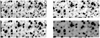 |
Fig. 2 Top left: reconstructed image of the data from 20 subsequent spectra. Top right: vista Variables in the Vía Láctea KS-band image cutout of the same region resampled to the pixel scale of 0.18 arcsec pixel−1. Bottom row: same as top row but convolved with a Gaussian PSF with an FWHM of 1″. The images cover ∼59″ × 22″ (2.3 × 0.9 pc). |
2.3 Astrometric calibration
To identify the location of a star on the two-dimensional spectral frames, we required an astrometric calibration. We used the Vista Variables in the Vía Láctea (VVV) survey (Saito et al. 2012) KS-band image (b333) as an astrometric reference. The image has a pixel scale of ∼0.34 arcsec pixel−1 and covers our entire field of view (FOV). We constructed stitched images from our spectroscopic observations and cross-correlated them with the reference image. This was done as follows:
We have 20 series of observations, with 6–22 exposures per series. These were taken without interruptions due to sky or telluric observations; hence, they cover continuous regions. Since each series contains the data from six slitlets, we constructed 20 × 6 = 120 stitched images by summing the flux in the wavelength range of 2.05–2.29 μm. The stitched images conserve the pixel scale along the slit (0.18 arcsec pixel−1), which is in the Galactic east-west direction. With the F2 pixel scale, each exposure covers six pixels in the north-south direction (6 × 0.18 arcsec≈1′′.1,), taking into account the drift. Each stitched image extends over ∼59″ (∼2.3 pc) along the Galactic east-west direction and over ∼6′′.5–24″ (∼0.25–0.9 pc) along the Galactic north-south direction, depending on the number of exposures. An example of such a stitched image is displayed on the top left of Fig. 2.
We know the approximate position of each stitched image, and we registered their centre position on the VVV image. We cut out the regions covered by the stitched images from the VVV image, leaving an additional 30 pixels (∼10″) on each side. We resampled those cutouts to the same pixel scale as the F2 data (0.18 arcsec pixel−1). Both the VVV cutouts and F2 images were convolved with a Gaussian point spread function (PSF), with the FWHM of 1″, and then cross-correlated to find the remaining small shifts, usually only a few F2 pixels. We then updated the headers of the stitched F2 images with the new astrometry. We show a reconstructed F2 image, a VVV cutout of the same region, and the convolved image versions in Fig. 2. A complete mosaic of all the reconstructed images is shown in Fig. 1.
2.4 Star extraction
To extract the spectra of bright stars, we used a star catalogue with information on the coordinates and JHKS band photometry. We used the GALACTICNUCLEUS (GNS) catalogue (Nogueras-Lara et al. 2019) with minor adjustments.
For our extraction method, completeness is more important than photometric precision and accuracy. As bright stars can be saturated in GNS data, the photometry of ∼25 stars in the F2 FOV was replaced with SIRIUS IRSF (Nagayama et al. 2003; Nishiyama et al. 2006) photometry, which was also used for the photometric calibration of the GNS catalogue. For another ∼400 stars in the central 40″ × 40″, we replaced HKS photometry with deep adaptive optics imaging from the instrument NACO at the ESO VLT (Schödel et al. 2020), as these data have a superior spatial resolution. Another 67 bright stars (J<17 mag or H<15.3 mag) have no KS photometry in either catalogue (possibly due to saturation), and we used the available J or H photometry to estimate it. We assume that the intrinsic colour (H − KS )0 = 0 mag, and that the stars are located in the GC. Hence, we can use an extinction map (see Sect. 3.4 for details), assume an extinction coefficient αHK = 2.23 (and αJH = 2.44, Nogueras-Lara et al. 2020b), and get a KS estimate from KS ≈ H − AH + AKS . These stars are later considered to be stars with an unknown status (see Sect. 3.5). Still, it is important to include these bright stars in the catalogue used for the spectrum extraction to ensure that they are accounted for and do not contaminate the spectra of nearby fainter stars.
The procedure to extract stars is as follows: for each of the 120 stitched images, we selected stars in the photometric catalogue that are located in the region of the stitched image. Knowing where the brightest stars are, we can derive the seeing in each stitched image. We fit a Gaussian function at the location of the ∼50 brightest stars per stitched image, along the slit directions. The mean value of the FWHM is used as seeing. The median seeing of our data is 0′′.8.
Next, we selected stars up to KS <15 mag, located again in the region of the stitched images, and up to 2″ beyond. We sort them by magnitude, starting with the brightest star. For each of these stars, we create an artificial image of the star in the sky, in an array of the same size and sampling as the F2 stitched image, with an FWHM corresponding to the previously measured seeing. The sum of the artificial images resembles the stitched image in terms of size, but it has the F2 sampling of 0.18 arcsec·pixel−1 in both dimensions.
For each star, again starting with the brightest one, we selected the spectral exposures that likely contain the flux of said star. We first considered the exposure that covers the position where the star is located, but due to the seeing, a star can contribute flux to several exposures. For this reason, we also considered the exposures taken before and after (i.e. three exposures per star). For stars fainter than KS =13 mag, we used only the primary exposure that covered the location of the star and the closest adjacent exposure (taken either before or after).
Starting with the primary exposure, we performed a Gaussian fit to obtain the exact location of the star on the slit, and its Gaussian σ. The extraction window was, by default, 6σ wide. Using the knowledge of the position and brightness of other stars in the field, we checked where other stars contributed more flux than the target star, and we reduced the extraction window accordingly if this was the case. The same procedure was repeated with the adjacent exposures that also contained the light of the star, but the Gaussian fit result of the primary exposure was used as an initial guess in the Gaussian fit. To extract a one-dimensional spectrum, we computed the total flux in the extraction window. We extracted 30 000 spectra of stars with KS <14 mag. We resampled each spectrum to its respective corrected wavelength calibration (see Sect. 2.2.2).
During the extraction process, we created masks of bright stars and foreground stars, and we used those to create data cubes of the unresolved faint stars. These data will be shown in a separate publication (Feldmeier-Krause et al., in prep.).
2.5 Spectral resolution
The spectral resolution of the F2 spectrograph varies across the detector, both as a function of position on the slit, and more significantly as a function of wavelength2. We measured the resolution by fitting a Gaussian function with width σLSF to the sky emission lines on the dedicated sky exposures after the rectification step. We used 14 sky emission lines in the range 2.001–2.252 μm. At shorter and longer wavelengths, there are no isolated emission lines suitable for a Gaussian fit. We performed these fits also as a function of the spatial slit direction. As expected, we found that the variation of the spectral resolution as a function of slit position at a given sky emission line is relatively small (σR(x)∼200, or 0.22 Å) compared to the variation along wavelength (σR(λ)∼700, or 0.96 Å) at a given slit position. Yet, as there is some variation along the slit, we decided to derive six different spectral resolution functions for the six different slitlets, resulting in a resolution variation for a slitlet σR(x)∼90, or 0.1 Å. In each slitlet region, we made a second-degree polynomial fit to the spectral resolution as a function of wavelength. The spectral resolution is highest at wavelengths of 2.1–2.2 μm with σLSF∼2.6 Å or R ∼3400.
3 Analysis
3.1 Spectral indices
As a first step in the spectral analysis, we derived the line-of-sight velocity VLOS, corrected the spectrum to the rest frame, and measured spectral indices, which help distinguish hot OB (early-type) stars from cool KM (late-type) giant stars. We measured VLOS using PPXF (version 5.2.1, Cappellari 2017), a fullspectral fitting code, in the wavelength range 2.15–2.3155 μm. This region includes H I Brackett (Br) γ, a Na I doublet, a Ca I triplet, and the CO 2–0 band head. We used the high-resolution spectral library of late-type stars provided by Wallace & Hinkle (1996) and a set of KMOS B-type dwarf stars (Feldmeier-Krause et al. 2020), and we convolved the templates to the spectral resolution of the data (as measured in Sect. 2.5). In particular, PPXF assigns weights to the template spectra, and the linear combination gives an optimal template for each fitted spectrum. Uncertainties were estimated by adding random noise to the spectra and repeating the fits in 80 realisations. The median VLOS uncertainty for all spectra is 11 km s−1, and when we applied a quality cut on the required S/N>20, the value was 6 km s−1.
After applying the VLOS shift to the spectra, we measured the following spectral indices – alternatively called equivalent width (EW): Br γ, which can be in absorption or emission in earlytype stars (as defined by Fritz et al. 2021); the CO 2–0 band head (∼2.2935 μm); the Na I doublet (2.2062 and 2.209 μm); and the Ca I triplet (2.2614, 2.2631, 2.2657 μm), which are seen in absorption in cool late-type stars (as defined by Frogel et al. 2001). We show example spectra in Fig. 3. In the figure, spectral features are indicated as vertical lines, and the spectral regions of the index measurements are highlighted by different colours.
We repeated the same measurements on the subset of Milky Way spectra of the X-SHOOTER spectral library (XSL DR2, Chen et al. 2014; Gonneau et al. 2020), convolved to the median spectral resolution function of the F2 data, to have a calibration sample. However, in these data, the change from one to the next Echelle order is at the location of the CO and Ca I spectral index continua, sometimes causing biased index measurements. Therefore, we also used the spectral libraries of Wallace & Hinkle (1996, 1997) and Winge et al. (2009). These data revealed that EWCO of giant stars at the F2 spectral resolution less than 25 Å, but supergiants can have EWCO>30 Å (as found at slightly higher spectral resolution by Feldmeier-Krause et al. 2017a).
We show the spectral index distributions of the spectral libraries and our data in Fig. 4. There is a larger spread in our data because of multiple reasons: our data has lower S/N than the spectral libraries, even after applying an S/N cut (more than 20). There can be sky residuals in the region of the CO feature, causing very low or high values; Spectra were not cosmic-ray corrected, to prevent the over-correction of bright star spectra (see Sect. 2.2); in particular the Br γ index is affected by interstellar gas emission, causing very low negative values. We note that for a given EWCO, the F2 data tend to have higher EWNa and EWCa, something that was already noted by Blum et al. (1996) and Feldmeier-Krause et al. (2017a) for GC stars, and hints at enhanced chemical abundances compared to Milky Way disc stars.
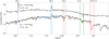 |
Fig. 3 Example spectra of a hot star (top) and a cool star (bottom). Both spectra are normalised by their median flux, and a small offset is added to improve visibility. The vertical lines indicate several spectral features used for the analysis, labelled on the top. Both spectra have Br γ emission due to surrounding gas (the hot star has even He I emission), but only the cool star has strong Na I, Ca I and CO 2–0 absorption features, and plenty of other metal lines. The regions used to measure the spectral indices are marked by different colours in the cool star spectrum, solid lines for the feature, and dotted lines for the pseudo-continuum regions. We annotate the KS and S/N (computed using the PPXF fit residual) for each star. |
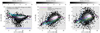 |
Fig. 4 Spectral EW of Br γ, Na I, and Ca I as a function of the EW of CO 2–0. The density maps show measurements on our extracted spectra after a quality cut on the required S/N. The green x-symbols are ∼100 stars in the Wallace & Hinkle (1996, 1997) and Winge et al. (2009) spectral libraries, and the blue plus-symbols are >400 Milky Way stars from Gonneau et al. (2020). Magenta solid lines, green dashed (for Wallace & Hinkle 1996, 1997; Winge et al. 2009), and orange dot-dashed lines (Gonneau et al. 2020) show the robust mean as function of EWCO. Stars with a Br γ measurement below the dot-dashed horizontal blue line in the left panel are affected by Br γ gas emission at the centre of the NSC. |
3.2 Stellar parameters
As the next step, we fit the stellar spectra extracted in Sect. 2.4 with the full spectral fitting code STARKIT (Kerzendorf & Do 2015; Do et al. 2015) using the PHOENIX spectral library of synthetic spectra (Husser et al. 2013) as templates. STARKIT interpolates the template spectra and applies Bayesian sampling (Multinest v3.10, pymultinest v2.11; Feroz & Hobson 2008; Feroz et al. 2009; Buchner et al. 2014; Feroz et al. 2019) to obtain the best-fitting parameters. We fit the total metallicity [M/H], effective temperature Teff, surface gravity log(g), and, in addition, the line-of-sight velocity VLOS. We ignored that the stars in our sample can have a range of chemical abundances (Thorsbro et al. 2020) and fit only the overall metallicity [M/H] as a parameter. This means the synthetic model spectra are computed with [α/H] = [M/H], and [α/Fe] = 0 dex.
We used the same constraints, limits, and bounds as in our previous works (Feldmeier-Krause et al. 2017a, 2020; Feldmeier-Krause 2022). In detail, the template spectra sample a grid with the ranges [M/H] = [−1.5 dex, +1.0 dex], Teff = [2300 K; 12 000 K], and log(g) = [0.0 dex, 6.0 dex], and with step sizes of △[M/H] = 0.5 dex, △Teff = 100 K, and △ log(g) = 0.5 dex. Before the fit, we convolved the template spectra to the spectral resolution of the data, as measured in Sect. 2.5. As fitting bounds, we used information obtained in Sect. 3.1, in particular, the value and uncertainty of VLOS in a Gaussian prior. The CO index measurement can be used to limit the uniform prior bounds of log(g). Giants in the spectral libraries have always EWCO<25 Å, and only supergiants have EWCO>25 Å. For ∼20 stars with EWCO>25 Å that are also brighter than KS,0=10 mag (extinction corrected), we used 0.0 dex < log(g) <2.0 dex; for all other stars we used a more generous 0.0 dex < log(g) <4.0 dex, as they may be giants or supergiants. The priors for Teff and [M/H] were uniform within the ranges of the PHOENIX spectra. We fit the spectral region 2.09–2.29 μm, but excluded the regions around the Na I doublet (2.2027–2.2125 μm) and Ca I triplet (2.2575–2.2685 μm), as these are enhanced in GC stars compared to normal Milky Way disc stars (as also shown in Fig. 4), and would bias our [M/H] to higher values.
After fitting the spectra, we computed the residuals by subtracting the best-fit model from the data and subsequently estimated the signal-to-residual ratio. We discarded fits with S/Nr<20, and also fits with large statistical uncertainties (σ(Teff)>250 K, σ(log(g))>1 dex, σ([M/H])>0.25 dex, σ(VLOS)>10 km s−1), which indicate either a poor fit or hot star candidates (see Sect. 4). When we had several spectra and goodquality fits of the same star, we combined the stellar parameter measurements with a simple mean. We used either the sum of statistical uncertainties in quadrature or the standard deviation of the multiple measurements as our new statistical stellar parameter uncertainty, depending on which is larger.
We compared our measurements with the literature in Appendix B.1 and found no strong biases. While the statistical uncertainties for Teff and log(g) are underestimated, the statistical uncertainty for [M/H] is a good approximation. We need to consider systematic uncertainties to estimate the total uncertainty. We estimated the systematic uncertainties caused by, for example, the choice of the synthetic model grid or variations of the elemental abundances in the stars by following the procedure outlined in Feldmeier-Krause (2022) and summarised in Appendix B.2.
3.3 Velocity corrections
The measured line-of-sight velocities VLOS are affected for instance by the motion of the Earth around the Sun, and also by the motion of the Sun around the GC. We computed a barycentric correction, which takes into account the rotation of the Earth itself, the rotation around the Earth-Moon barycentre, and the rotation around the Sun by considering the individual coordinates of each star, the time of the observation, and the coordinates and altitude of the telescope with the IDL program HELCORR.PRO, which uses the algorithms of IRAF NOAO.ASTUTILS.RVCORRECT. The barycentric correction ranges from –5.5 to –2.3 km s−1.
Perspective rotation is an effect caused by the large extent of the data on the sky and the substantial motion of the Sun around the GC. This causes a so-called perspective rotation and increases the difference between the motion of stars in the very east and very west by almost 2 km s−1. We computed the effect with the equations given by van de Ven et al. (2006) and assuming a distance of 8.2 kpc, a velocity of 220 km s−1 of the Sun in the Galactic plane, and –7 km s−1 perpendicular to it. The latter motion is negligible, causing only a perspective rotation of ∼0.003 km s−1 in the FOV of the data. The correction for the motion in the Galactic plane is in the range of –0.95 to +0.95 km s−1.
3.4 Extinction map
We created an extinction map using the photometric data of the GNS. We follow the procedure outlined in Nogueras-Lara et al. (2018) and also applied in Feldmeier-Krause (2022). In brief, we selected all GNS stars in the region of our spectroscopic F2 data and several arcseconds beyond. Of these, we selected the likely red clump stars, which have a colour 1.3 mag<H − KS<2.6 mag, and we applied colour-dependent magnitude cuts as shown in Fig. 2 of Feldmeier-Krause (2022). Using Eq. (5) of Nogueras-Lara et al. (2018), and assuming the same filter effective wavelengths, intrinsic colour for the red clump stars ((H − KS )0=0.089 mag), and extinction coefficient (αJHKS =2.3), we derived the extinction AKS for each red clump star. From these, we derived an extinction map (with pixel scale 0.1797″·pixel−1) by computing in each pixel the distance weighted mean AKS of the 15 closest red clump stars within 12 arcsec. Our extinction map has a mean value of AKS = 2.1 mag with a standard deviation of 0.22 mag. The values of AKS range from ∼1.5–2.7 mag.
3.5 Galactic centre membership classification
We use simple colour cuts to classify stars that are likely located within the GC structures NSC and NSD, or foreground stars, or background stars. In detail, we identify a star as a foreground star if H − KS ≤ 1 mag (as in Clark et al. 2021), and as a background star if H − KS ≥ 3.5 mag. Stars for which either H or KS are missing are classified as unknown. We refer to the combination of these three groups of stars (foreground, background, unknown) as non-GC stars. Our classification criteria are rather inclusive compared to other studies, which classified stars as foreground stars if H − KS ≲1.3 mag (e.g. Fritz et al. 2016; Feldmeier-Krause 2022). These studies have smaller fields of view, with less variation of the foreground extinction. Using the stricter criterion on the foreground only removes 70 stars with stellar parameter measurement, which is less than 3% of the sample, and has no influence on our results. We show the colour-magnitude density diagram of the cool late-type stars in Fig. 6, the left panel before extinction correction versus the right panel after extinction correction in the GC.
We estimate the contribution of the bar, the NSD, and the NSC as a function of longitude in our FOV using the AGAMA package (Vasiliev 2018, 2019). Sormani et al. (2022) give estimates of the bar contribution in various regions of the NSD beyond our observed fields. In the fields closest to our data, though still several parsec away, the surface density contribution of the bar compared to the total surface density of the bar and NSD is 19–26%. We estimate that the bar contribution is less than ∼20% in our field. We further used the stellar density profiles of Chatzopoulos et al. (2015) for the NSC and Sormani et al. (2022) for the NSD (see Fig. 5, top panel), and compared the projected surface density profiles (i.e. integral of density along the line-of-sight) at the location of our data. Assuming a spatially constant bar contribution, we find that the value of Galactic longitude where the NSC surface density contributes more than 50% of the total (NSC+NSD+bar) density is at l ≲7.7 pc for b=0 pc, and l ≲7.2 pc for b=2 pc (see Fig. 5, bottom panel). Further out, the NSD dominates the projected stellar surface density. However, we made several assumption: we assumed that the bar contribution is a simple extrapolation from Sormani et al. (2022), we did not consider the orientation of the bar, and we neglected potential observational biases caused by varying extinction. Nonetheless, these estimates helped us understand where the NSC or the NSD likely dominate our sample.
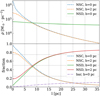 |
Fig. 5 Stellar surface density profile in the GC. Top panel: NSC profile from Chatzopoulos et al. (2015), NSD profile from Sormani et al. (2022) as a function of l. Bottom panel: fraction of the NSC and NSD density profiles, if the bar density profile is constant, and set to 20% of the NSD density profile at l = 35 pc and b = 0 pc. |
4 Hot star candidates
The strength of CO absorption decreases with increasing Teff (Kleinmann & Hall 1986; Feldmeier-Krause et al. 2017a). A spectrum without CO absorption indicates a hot and, given the brightness of our sample, young and massive star. We classify a star as a hot star candidate if EWCO ≲ 5 Å. Sometimes noise or sky line residuals contaminate our CO measurement. Hence, we visually inspected the spectra, and in some cases, we classified stars as hot candidates even though the value of EWCO exceeds the above threshold, as bad pixels affect the measurements. We list these 78 stars in Table E.5. This list includes stars with visible but weak CO absorption (EWCO> 0 Å). Due to our poor spatial resolution, it may be possible that the detected weak CO absorption is caused by contamination of nearby late-type stars rather than from the star itself. Hence, we list these stars as potential hot stars. If the CO absorption is intrinsic to the star, it is likely a rather warm giant.
We verified our hot star candidates by comparison with the literature, notably with the early-type candidates of Feldmeier-Krause et al. (2015); Feldmeier-Krause (2022), but also the late-type stars in Feldmeier-Krause et al. (2017a, 2020). Feldmeier-Krause et al. (2015) identified >100 young stars in the central 4 pc2 around Sgr A★, and we identified 15 candidates in this region. We matched stars with a maximum distance of 0′′.3 and found 15 matches in the Feldmeier-Krause et al. (2015) data. We have two additional candidate stars with EWCO ≈4.6 Å in the same FOV, but they were classified as late-type stars in Feldmeier-Krause et al. (2017a). We mark these stars with a footnote in Table E.5. These stars are fainter (KS ∼13 mag) than the rest of our matches. As Feldmeier-Krause et al. (2015) and Feldmeier-Krause et al. (2017a) have a better spatial resolution (seeing limited) than we do (>1″ along latitude), their classification is less likely to be contaminated by background sources. We also matched two hot stars (within even <0′′.1) with Feldmeier-Krause (2022), which cover two 4 pc2-sized fields located about 20 pc east and west of Sgr A★. Our matches correspond to the two brightest out of the nine hot stars in Feldmeier-Krause (2022). This comparison shows us that we can identify bright hot stars reliably.
We show the spatial distribution of the hot star candidates in Fig. 7. As noted in other spectroscopic studies (Feldmeier et al. 2014; Feldmeier-Krause et al. 2015; Støstad et al. 2015), we find that the young stars are concentrated in the central ∼1 pc region around Sgr A★. Beyond this region, hot stars are rather sparse.
At a ∼20–30 pc distance from Sgr A★, we see a higher density of hot stars in the Galactic east compared to the west. These stars may be related to the Quintuplet cluster, one of the young star clusters in the GC (∼4 Myr, Figer et al. 1999; Liermann et al. 2012). Quintuplet is located only 30″ (∼1.2 pc) to the south of our FOV, and we have several hot star candidates just north of it (at ∼30 pc east of Sgr A★). If the stars are associated with Quintuplet, their proper motions should point in the same direction as the proper motion of the cluster. If some of these stars used to be associated with Quintuplet but were ejected (see Sect. 6.1), their proper motion should point away from the current or former position of the Quintuplet cluster. Quintuplet is on an orbit around the GC and moves mostly to the Galactic east and slightly towards the south.
We matched our hot star candidates with the proper motion catalogue of Shahzamanian et al. (2022). We list the 23 matches (within ≤0′′.2) in Table E.1. The proper motions are depicted as arrows in Fig. 7. All of these stars are classified as GC star via their H − KS colour (>1.34 mag). Some stars (e.g. F2_26652917-28857695_Ks12.95, F2_2665248428854546_Ks12.20, F2_26643866-28966084_Ks12.46) appear to have proper motions directing them away from Quintuplet’s orbit, so they may have been ejected.
We also have nine matches within ≤0′′.2 with the proper motion catalogue of Libralato et al. (2021), but only four are classified as GC stars (see Table E.2). Two stars also have proper motions in Shahzamanian et al. (2022), but the results are not consistent, which may be caused by the different reference frames used by these studies. Libralato et al. (2021) data are in the absolute Gaia reference frame, while Shahzamanian et al. (2022) are only relative proper motions.
In addition, we matched our data with the Quintuplet proper motion catalogue of Hosek et al. (2022), which covers only the very east of our data. However, the proper motions are more precise than those of Shahzamanian et al. (2022), and in the Gaia reference frame. We obtain 12 matches (coordinates match within ≤0′′.2), which we list in Table E.3 and show in Fig. 8.
From the nine stars that we classify as GC stars (marked by a red diamond), eight move roughly parallel to Quintuplet and with a similar amplitude. Only one of these stars was reported as a spectroscopic hot star in the stellar census of Quintuplet stars by Clark et al. (2018a) and is also a Paschen α source in Dong et al. (2011). Their proper motions, projected location within the tidal radius, and their spectral types make these eight stars likely Quintuplet members.
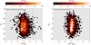 |
Fig. 6 Colour-magnitude diagram of the sample with stellar parameter fit. Left panel: observed H − KS versus KS diagram for all stars with a stellar parameter fit. The vertical dashed lines enclose the stars classified as being located in the GC. Right panel: extinction corrected (H − KS )0 versus KS,0 diagram of stars with a stellar parameter fit and classified as being located in the GC. |
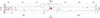 |
Fig. 7 Proper motions of stars in the FOV. Red-coloured diamonds denote hot star candidates we classified as being located in the GC, as listed in Table E.5, and blue cross-symbols denote those hot stars we classified as non-GC stars or stars with unknown status. The black arrows indicate the proper motions of hot star candidates from Shahzamanian et al. (2022). The arrow lengths are multiplied by a factor of 3000 for better visualisation. The grey arrows are a subset (2.5%) of the Shahzamanian et al. (2022) proper motions to illustrate the distribution of proper motions in this region. Black dashed lines denote the approximate outline of our FOV, blue dashed lines the region shown in Fig. 8. The purple circle denotes Quintuplet’s tidal radius rt ∼3 pc (Rui et al. 2019), the green solid circle denotes the NSC Re = 5 pc. The x-axis and y-axis have different scales; therefore, the circles and proper motions appear elongated along the y-axis. |
5 Late-type star stellar parameters and kinematics
After deselecting stars with low S/N and poor fits (Sect. 3.2), we obtain stellar parameters for 2715 stars, of which we classified 2580 as GC stars. We show their density distribution across our observed FOV in Fig. 9. Similar to what we see in Fig. 1, the stellar density is highest in the centre, around Sgr A★.
5.1 Stellar parameter distributions
We show the stellar parameter distributions of the 2580 GC stars for Teff, [M/H], and log(g) in Fig. 10. The values of Teff (left panel) are mostly 3000–4000 K and consistent with M-type red giant stars. The surface gravity log(g) (right panel) can hardly be constrained by our data but is also consistent with red giant stars.
The [M/H] distribution (middle panel) has a wide range, covering values from –1.5 dex to +1.0 dex, which includes the entire range of the model grid. Most stars have super-solar overall metallicity ([M/H] >0 dex). About one out of four stars even has [M/H] >0.5 dex. Our method derives the overall metallicity [M/H], meaning that all elements are considered in the measurement (not only Fe), and [α/Fe]=0 dex and thus [α/H]=[M/H] in the models. We note that very high iron abundances of [Fe/H]>0.5 dex have not yet been found in high-spectral resolution data (Do et al. 2018; Thorsbro et al. 2020; Ryde et al. 2025), and we could not calibrate if our method works at such high values. It is possible that high elemental abundances (as indicated by high EWCa and EWNa for a given EWCO, see Fig. 4) push the overall metallicity [M/H] measurement of GC stars to high values. Although we excluded the spectral regions around the Ca I and Na I lines from our [M/H] fit, other elements and lines in the spectra can indicate super-solar abundances (Do et al. 2018; Thorsbro et al. 2020). Thus, a value of [M/H] >0.5 dex is not only caused by iron. Nonetheless, such stars can be considered stars with super-solar metallicity.
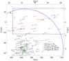 |
Fig. 8 Proper motions of stars in the region close to the Quintuplet cluster. Red-coloured diamonds denote hot star candidates we classified as being located in the GC, and blue cross-symbols denote those stars we classified as non-GC stars or stars with unknown status. The red arrows indicate the proper motions of our hot star candidates from Hosek et al. (2022). The arrow lengths are multiplied by a factor of 3000 for better visualisation. The grey arrows are a subset of the Hosek et al. (2022) proper motions, showing 33% of the stars with more than 80% cluster probability. Black dashed lines denote the approximate outline of our FOV. The dashed purple circle denotes Quintuplet’s core radius rc, the solid purple circle its tidal radius rt (adopted from Rui et al. 2019), and the purple arrow pointing at the centre denotes the direction of the orbit of Quintuplet (Fig. 6 in Hosek et al. 2022). Green coloured squares denote spectroscopic hot Quintuplet stars from Clark et al. (2018a), magenta triangles are Paschen α candidates from Dong et al. (2011). |
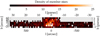 |
Fig. 9 Density of late-type GC stars with stellar parameter measurements, as a function of Galactic longitude and Galactic latitude, centred on Sgr A★. We have the largest density in the centre of our field, where the stellar density is also the highest. The higher density in the inner 5 pc east of Sgr A★ compared to inner 5 pc west of Sgr A★ is likely caused by the lower extinction of the east region (see also Fig. 12, bottom panel), and is already visible in the photometric catalogue. We note that the vertical axis is stretched relative to the horizontal axis of the plot to improve visibility. |
5.2 Stellar evolutionary stages
The extinction corrected KS,0 photometry (see colour-magnitude diagram, right panel in Fig. 6) helped us estimate the luminosity class of the stars. According to Blum et al. (2003), red supergiant stars located in the GC are normally bright (KS,0=5.7 mag), but can be as faint as KS,0=7.5 mag, which applies to only 50 of our GC stars. However, stars with KS,0 > 5.7 mag are most likely red giant branch (RGB) stars, and we conclude that the majority of the stars in our sample are normal red giant stars. All of them are brighter than the red clump, which is centred at KS ∼15.8 mag (for a mean extinction of AK∼2.6 mag, Schödel et al. 2020).
A few stars in our sample must be asymptotic giant branch (AGB) stars. They tend to be younger than RGB stars (∼1–2 Gyr, depending on their mass). The time a star spends on the AGB is about 40 times shorter than their time as an RGB star (Greggio & Renzini 2011). Hence, we expected ∼65 AGB stars in our sample. Via their variability, we identified 26 (39 including non-GC, coordinates match within <0′′.3) AGB Miras from the catalogue of Matsunaga et al. (2009), accounting for 41% of the expected AGB stars. In total, we found that 72 (100) of the stars in our GC (full) sample are listed as variable stars in Matsunaga et al. (2009), who could not obtain a period for all of them. Thus, it is unclear for several stars what causes the variability and if they are AGB Miras.
We also matched our sample with the variable star catalogue of Matsunaga et al. (2013) and found two matches (coordinates match within <0′′.2), which happen to be among the four warmest stars in our sample with Teff >4700 K (F2_2663787229052971_Ks10.57 and F2_26638443-29048691_Ks10.26 correspond to stars 18 and 20 in Matsunaga et al. 2013). These stars are classical Cepheids, that is, pulsating supergiants that evolved from intermediate-to-high-mass stars (4–10 M⊙).
5.3 Position-velocity diagram and high-velocity stars
We find on average rotation of the stars in the same sense as the Milky Way disc, with stars receding in the Galactic east and approaching in the Galactic west. We show 2580 stars (after the colour cut to remove non-GC stars) on a position-velocity diagram in Fig. 11. The red line denotes the moving average VLOS as a function of Galactic longitude l, computed using the nearest 150 stars. This curve is roughly symmetrical about l=0, and flat beyond the inner ∼100″ (3.9 pc), with an absolute value close to 25 km s−1.
The position-velocity diagram reveals several stars that move apparently in the opposite direction, and stars with large VLOS, exceeding 150 km s . We classify a star as a high-velocity star if it satisfies one of the following conditions:
located at a distance of r>50″ from Sgr A★, and |VLOS|>Vcut,1=200 km s−1,
at r>100″ from Sgr A★, and VLOS >Vcut,2=150 km s−1, if the star is located >100″ to the west of Sgr A★ (i.e. counterrotating in the West), or
at r>100″ from Sgr A★, and VLOS <−Vcut,2= –150 km s−1, if the star is located >100″ east of Sgr A★ (i.e. counter-rotating in the East).
The values of Vcut,1 and Vcut,2 are chosen to be symmetrical about the flat VLOS curve, and after visual inspection of the position-velocity curve. For comparison, the overall moving robust σ times a factor of 3 is ∼200 km s−1, the exact value depends slightly on the number of stars used for the moving average.
Even though these high-velocity stars are only a small number compared to the size of our data set, we excluded them as possible contaminants from further analysis. We discuss their potential origin in Sect. 6.2.
5.4 Stellar parameter maps
In this section, we study how the mean properties of the stars vary spatially. We apply Voronoi binning on the data (using the code provided by Cappellari & Copin 2003), such that nearby stars are grouped in bins of ∼40 stars each. We also tried different bin sizes (e.g. 30, 60, 100) but found consistent trends. A lower number of stars per bin naturally gives noisier maps, and a higher number of stars per bin washes out spatial differences. Then we computed the mean values of various parameters, such as extinction corrected KS,0-band photometry, observed colour H − KS , extinction AKS (see Fig. 12), Teff, [M/H], and log(g) (see Fig. 13). Maps of the median instead of mean value per bin show similar trends (i.e. regions with high or low values coincide). We also show the moving average profiles of 200 stars along Galactic longitude l in Figs. C.1 and 17, which show consistent trends.
Our maps show a region near the centre, located southeast of Sgr A★ (–1 pc<b<0 pc, 0 pc<l<+8 pc), where the stars are on average fainter, warmer, and have higher log(g) than for example the opposing northwest side of Sgr A★ (0 pc<b<+1 pc, −8 pc<l<0 pc), and also the northeast, and southwest sides. We compared the GNS catalogue and found that indeed, the southeast side of Sgr A★ has a higher density of stars with 10 mag<KS <12 mag compared to the west. The higher average values of several parameters (Teff, log(g), and KS ) in the southeast of Sgr A★ agree with expectations from red giant star evolution. Along the red giant branch, Teff decreases slightly while the total luminosity increases and log(g) decreases. Hence, if on average we detect fainter stars, it is natural that on average they have higher log(g) and are warmer. However, our uncertainties of Teff and log(g) are substantial, and quantitative comparison with isochrones is not meaningful. The inner –10 pc<l<10 pc region has higher extinction (AKS > 2.0 mag), which also causes the redder H − KS . A redder colour can indicate a larger line-of-sight distance dLOS, as redder stars lie behind a larger amount of interstellar dust.
As shown in Fig. 13, the mean metallicity,  , varies spatially. There appears to be an increase from the central r ≲1 pc region around Sgr A★ with
  = 0.06 dex (∼200 stars), towards the surrounding region (–5 pc<l<5 pc and –1 pc<b < 1 pc, ∼650 stars), with a
  =0.27 dex. Further,
  decreases towards the north at b ≳1 pc to 0.02 dex (∼500 stars). This trend can also be seen in Fig. 17 top panel, where the blue dashed line, indicating the region b< 1 pc, has higher
  than the orange line, denoting b> 1 pc. All these regions are dominated by the NSC stars rather than the NSD stars according to the projected surface density (Sec. 3.5). The lower
  found in the north is in agreement with the larger fraction of sub-solar [M/H] stars in the Galactic north compared to the south reported in Feldmeier-Krause et al. (2020). While our data in the north extend even further than the data of this study, we have no coverage in the south at b< –1 pc.
At |l| ∼2–8 pc, and b ∼0 pc,  decreases on both sides of the NSC. This decline does, however, not continue into the inner NSD, and from 10 pc outw ards, where the NSD is dominating the stellar density (Sect. 3.5),
  is rather constant on both sides. There appears to be a slight east-west asymmetry, with
  =0.15 dex at l>10 pc (∼450 stars, east) and
  =0.26 dex at l<– 10 pc (∼400 stars, west). In these regions, the contribution of the NSC to the stellar surface density is below 50%. At l>10 pc and l<–10 pc, we find a similar level of foreground extinction (AK ∼1.8–2.0 mag), which is lower than in the NSC-dominated area (2.1–2.4 mag).
The distribution of [M/H] is broad, with σ[M/H]=0.43–0.47 dex. However, the variation of  is likely too large to be caused by randomly drawing a finite number of stars from the entire sample. We tested this by drawing 1000 random samples from the [M/H] distribution (after removing high velocity and foreground stars) of our data, with varying sample sizes (40–200 stars). For each sample, we compute
  , and the resulting value is always close to the overall
  , 0.17 dex, even if we draw only 40 stars. As expected, the standard deviation of the 1000 simulated sub-samples decreases with increasing sample size. We computed how likely it is to obtain the values of
  stated above for the different regions and for the given number of stars: obtaining
  =0.06 dex (as found in the central 1 pc) when drawing 200 stars randomly from the data set is 3.5σ below the expected value, while
  =0.27 dex (as in the surrounding region, for 200 stars) is 2.8σ above. If we draw random samples only from the stars in the inner <8 pc, we obtain – 2.9σ and +3.5σ, respectively. If we allow the individual [M/H] measurements to vary within their respective total uncertainties σ[M/H], the significance is slightly lower, 2.2σ and 2.5σ.
This suggests that the null hypothesis that there is no spatial variation of the  distribution (even only in the inner <8 pc) can be discarded, and there is a real spatial variation of [M/H] in the data. The east-west asymmetry is less significant, with only 1.6σ and 0.9σ (for 200 stars and if considering individual [M/H] uncertainties). We discuss possible explanations for the variation of
  in Sect. 6.4.
We further analysed the different regions with one-dimensional Gaussian mixture models (GMMs). We tested single and double Gaussian models and used the Bayesian information criterion (BIC) and the Akaike information criterion (AIC) to decide which is a better representation of the data. In all regions except the centre, a double Gaussian gives a better fit to the data. We list the resulting Gaussian centres, widths, and relative weights of the first double-Gaussian in Table 2 for the different regions (the corresponding histograms are shown in Fig. D.1). We obtained uncertainties by running Monte Carlo simulations with 1000 different data representations. We used the statistical uncertainty σ[M/H] to draw modified values of [M/H] for each star in the regions and repeated the GMM analysis. The standard deviation of the 1000 runs is listed as the uncertainty of the GMM, and the mean as the value. Using the mean of the MC runs rather than the actual value increases [M/H]2 and the Gaussian widths σ[M/H]1,2.
The east and west regions are similar, though the east region has a larger weight at the low [M/H] Gaussian, and the second component is centred at lower [M/H] compared to the west region. In comparison to all other regions, the north region has the lowest [M/H] values for both Gaussian components, reflecting the lower values of  in this region. The central (r < 1 pc) region is the only one where a single Gaussian gives better results than a double Gaussian. The region surrounding the innermost r=1 pc has indeed the highest [M/H] of all regions for both components, confirming what we see for
  in Fig. 13. This is caused by a relatively large number of stars with very high [M/H] >0.5 dex, which may be overestimated (see Sect. 5.1). The widths of the first components are similar everywhere (σ[M/H]1 =0.48–0.60 dex), and broader than that of the second, higher [M/H] components (σ[M/H]2 =0.35–0.49 dex). Overall, the GMM analysis confirms our findings of a spatially varying [M/H] distribution, with lower [M/H] in the north, the central r < 1 pc, and higher [M/H] in the surrounding (r > 1 pc) region.
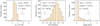 |
Fig. 10 Stellar parameter distributions of GC stars. From left to right panel, effective temperature Teff, overall metallicity [M/H], and surface gravity log(g). We denote the mean, median, and standard deviation of the distributions on each panel, and we show the mean statistical and total uncertainty with a cross and diamond symbol. |
 |
Fig. 11 Position-velocity plot of GC late-type stars along Galactic longitude, centred on Sgr A★. Each diamond symbol denotes a star, and green x-symbols denote stars that we consider high-velocity stars. The red line denotes the moving average VLOS of 150 stars, the blue lines denote the moving robust σr × 2.5, which is close to our cuts to classify high-velocity stars, shown as dashed horizontal lines. |
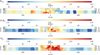 |
Fig. 12 Mean photometric properties in different Voronoi bins: KS,0 (top), H − KS (middle), and AKS ,0 (bottom). The mean KS,0 indicates that the stars in the central region are slightly fainter than stars in the outer regions, especially in the west. The stars in the centre are slightly redder (higher mean H − KS ), and in this region, the extinction AKS is higher. High-velocity stars and foreground stars were excluded. Each bin contains ∼40 stars. |
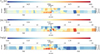 |
Fig. 13 Mean effective temperature Teff, overall metallicity [M/H], and surface gravity log(g). The regions with fainter stars in Fig. 12 (top panel) have higher Teff and log(g), as expected. High-velocity stars and foreground stars were excluded. Each bin contains ∼40 stars. |
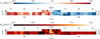 |
Fig. 14 Mean line-of-sight velocity VLOS (top) and velocity dispersion σLOS (bottom) in bins of ∼40 stars. High-velocity stars and foreground stars were excluded. |
Gaussian mixture model of the [M/H] distribution in different regions.
5.5 Stellar kinematic maps and variations
The stars in the NSC and NSD rotate in the same sense as the rest of the Galaxy, with Sgr A★ in the centre. In Fig. 14, we show maps of the mean VLOS (top) and velocity dispersion σLOS (bottom) in bins of ∼40 stars each. Foreground stars and high-velocity stars (Sects. 3.5, 5.3) were not considered for these maps. The σLOS map has a maximum in the innermost bin (∼90 km s−1), this marks the typical σLOS increase around a supermassive black hole. Further out, σLOS is rather constant at ∼62 km s−1.
Since the stars have a broad [M/H] distribution, it is interesting to check if the stellar kinematics shows any dependence on [M/H]. We made position-velocity plots along Galactic longitude l, and binned the data according to their [M/H], see Fig. 15, top panel. In each [M/H] bin, the stars show a rotation signature. There is more variation in the Galactic east among different [M/H] bins, and the moving average value of VLOS has a standard deviation of up to ∼10 km s−1, while it is below 5 km s−1 in the west. The velocity curves agree within their uncertainties in the west but show some deviation in the east, exceeding the uncertainties. As a consequence, the velocity curves are not perfectly symmetric about Sgr A★. We quantify this deviation from asymmetry by calculating the median difference of the absolute value of VLOS on the two sides and the robust standard deviation. The numbers tell us that the 0.35 dex<[M/H] <0.6 dex bin has the largest deviation from symmetry, with a median difference of 17.7 km s−1, while all other [M/H] bins have <5 km s−1. This [M/H] bin has the lowest velocity on the east side from all the [M/H] bins, which is the reason for the asymmetric VLOS curve. We cannot detect a variation of the VLOS curve with [M/H] as seen by Schultheis et al. (2021) in the NSD, at larger distances (l ≲200 pc) from Sgr A★ than our data. Schultheis et al. (2021) found that stars with increasing [M/H] show a stronger rotation signal, but we see no significant differences in VLOS with [M/H] in the west, and differences in the east do not show such a trend in our data. These trends do not change if we use a stricter colour cut to exclude foreground stars (e.g. H − KS <1.3 mag instead of 1.0 mag), and exclude more stars as high-velocity stars (e.g. |VLOS |>120 km s−1 instead of 150 km s−1). The stars in the inner r<2 pc have a velocity dispersion ranging from 71–85 km s−1. Stars in the highest [M/H] bin have the lowest velocity dispersion value, and stars with [M/H] <0.1 dex the highest. This may indicate slight differences in the projected distance of the stellar samples to Sgr A★.
We also make a position–velocity plot (running average of 100 stars) where we bin stars according to the observed H − KS colour (bottom panel of Fig. 15), and there we see significantly larger variations. The stars with the bluest colour (212 stars, 1.0 mag<H − KS <1.6 mag) show the weakest rotation signal, with |VLOS| ≲ 16 km s−1. Stars with 1.6 mag<H − KS <2.0 mag (834 stars) do show stronger rotation (up to |VLOS| ∼45 km s−1), but the maximum |VLOS| are at the outermost values of l. We observe a strong |VLOS| peak at 46 km s−1 in the inner l<4 pc for the 2.3 mag<H − KS <2.6 mag bin (474 stars). The neighbouring colour bins, 2.0 mag<H − KS <2.3 mag (635 stars) and 2.6 mag<H − KS <3.5 mag (343 stars) show indications for such a peak, but less pronounced.
Besides the variation of the maximum |VLOS| and its position, we note that the stars with bluer H − KS are more extended along l, while the stars with redder H − KS can be found predominantly in the centre, in agreement with the mean H − KS map shown in Fig. 12, middle panel. Stars with red colour (H − KS >2.3 mag) have the highest velocity dispersion in the inner r<2 pc, σLOS >82 km s−1, stars with bluer colour (1.6 mag<H − KS <2.0 mag) have σLOS =71 km s−1, and the stars in the bluest bin only σLOS=39 km s−1. We discuss these results in Sect. 6.5.
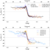 |
Fig. 15 Binned position–velocity plots of GC late-type stars after removing high-velocity stars, along Galactic longitude, centred on Sgr A★. Top panel: position–velocity curves for different [M/H] bins (moving average of 100 stars). Different colours and lines denote the different [M/H] selection (see figure legend). Bottom panel: same as top panel but applying bins in H − KS . |
6 Discussion
6.1 Hot star discoveries
We identified 78 hot star candidates, of which 48 are classified as GC stars based on their H − KS colour. Fifteen of these stars are located in the projected inner 1 pc region around Sgr A★, and those stars match the brightest of the hot young stars extensively studied in the literature (e.g. Krabbe et al. 1991; Paumard et al. 2006; Lu et al. 2009; Feldmeier-Krause et al. 2015; von Fellenberg et al. 2022).
We discovered 31 hot stars that were, to the best of our knowledge, not yet reported in the literature as hot stars. A larger number of these hot stars is located in the Galactic east, at l=30 pc, with 11 (and an additional four non-GC) sources just a few parsecs north of the Quintuplet cluster of young stars. Only one of these stars is listed as a spectroscopically confirmed hot star by Clark et al. (2018a). We tested if these stars may be associated with the Quintuplet cluster by matching them with the proper motion catalogue of Hosek et al. (2022). We found that indeed eight stars have similar proper motions to Quintuplet. The most distant star is ∼2.7 pc (projected on the sky) away from Quintuplet’s centre, and the closest one only ∼1 pc. Rui et al. (2019) identified 715 Quintuplet cluster members, as far out as 3.2 pc. They adopt a tidal radius rt=3 pc, and a core radius rc=0.62 pc. Hence, the eight stars co-moving with Quintuplet are within its tidal radius and are likely associated with it. We found no match in the proper motion catalogue for one of the stars, as it is likely outside of its FOV. One star (F2_2665403428827679_Ks11.74) is moving more northwards and is faster than the rest of the stars that co-move with Quintuplet. It may either not be part of the cluster, or some dynamical event (e.g. a close encounter, kick) may have changed its proper motion.
There are several rather isolated young stars in our FOV, with no association to the known young star clusters. Seventeen GC stars are located outside Quintuplets tidal radius or the NSC’s Re. Only two of them were already reported as spectroscopic hot stars in Feldmeier-Krause (2022). Nonetheless, their discovery is unsurprising, as several studies also found young massive stars throughout the GC. Most of the known isolated hot stars were discovered thanks to Paschen (Pa) α excess, caused by emission lines (Mauerhan et al. 2010a; Dong et al. 2011, 2015; Clark et al. 2021). These stars are either Wolf Rayet stars, O hypergiants, or luminous blue variable stars. Clark et al. (2021) discuss that Pa α surveys can miss mid-O supergiants, and detect no O5-9 stars of luminosity class III to V. Our hot star candidates are not limited to emission line stars, and the stars in our sample can have Brγ absorption. Thus, our sample likely includes different spectral types of stars, including O and B giants to main sequence stars. Indeed, 17 of our isolated hot stars in the GC (26 including stars close to the centre and Quintuplet) are in the range of KS,0 = KS − AKS =10–12 mag, which makes them probably O3V – B0V stars (Pecaut et al. 2012; Pecaut & Mamajek 2013). Such stars have no emission lines, which explains why the Pa α survey did not detect them.
Some of the isolated hot stars have proper motions from Shahzamanian et al. (2022) that are, however, neither parallel to Quintuplet’s proper motion nor aligned with its orbit, as would be expected from a tidal tail (Habibi et al. 2014). Also, Rui et al. (2019) did not detect tidal tails for Quintuplet, but Park et al. (2018) showed that tidal tails are barely detectable via massive stars, as most stars in the tidal tail have masses less than 2.5 M⊙.
A possible mechanism to eject a hot star from a star cluster is a three-body interaction of a single star with a binary or a multiple system. According to Gvaramadze & Gualandris (2011), in more than 50% of encounters of a massive star (12– 20 M⊙) with a massive binary, the star is accelerated, typically to ∼90 km s−1. Slightly higher velocities can be reached if a binary system evolves into a supernova (SN) and ejects a star. Quintuplet and the central parsec cluster are old enough for this process, while Arches is too young. If three-body interactions and SNe ejections generate runaway kicks of ∼100 km s−1, a star can be displaced by ∼100 pc within 1 Myr (Clark et al. 2021). This is less than the age of the young clusters and therefore makes them potential sources for some of the isolated massive young stars found throughout the GC.
Then, there is also the possibility that the isolated young stars formed in small groups that are already dissolved, or even in true isolation (Dong et al. 2015). Stars from dissolved clusters or groups are expected to retain information on their kinematics and move with similar velocities. Such co-moving groups of stars were reported by Shahzamanian et al. (2019); Martínez-Arranz et al. (2024). A better estimate of their kinematics and spectral type would be useful to constrain the origin of these isolated hot stars. With higher-quality spectra at a better spatial resolution than our data, it should be possible to constrain the spectral type and luminosity class of the stars and, in addition, measure their VLOS.
6.2 High-velocity star origin
Our sample contains several stars that move with a high VLOS, some of them even in the opposite sense than the bulk of the stars. The high-velocity stars have lower [M/H]-values than the slower stars. The mean value of [M/H] of the 82 high-velocity stars is –0.21 dex, the median even –0.27 dex, significantly less than the mean and median of the other ∼2500 stars, +0.17 dex and +0.22 dex. The observed colours H − KS and J − KS are on average less for the fast stars, with mean values of 1.87 and 7.50 mag versus 2.13 and 9.98 mag, indicating that they may be on average closer to us along the line of sight, lying in front of some of the GC dust. However, the distributions of Teff, log(g), or K0 are not significantly different.
One possibility for the origin of these stars is that they belong to the Galactic bar. For such stars, we expect the mean VLOS close to 0 km s−1 at the location of our data, but also a large velocity dispersion of ∼120 km s−1 (Portail et al. 2017a,b). If a star is on an x1 orbit in the bar, it moves along the bar’s long axis, which is oriented at an angle of α=28°–33° (Wegg et al. 2015). If the star is moving outwards, the star’s VLOS has the opposite sign than the VLOS of stars in the NSD and NSC, which are rotating around Sgr A★. In this case, the star would appear as counter-rotating. The star turns around and moves inwards after reaching the apocentre of its orbit, leading to an apparently co-rotating VLOS. Stars in the bar have lower [M/H] than stars in the GC (Schultheis et al. 2019), which is also in agreement with our findings. Given that we expect a bar contribution of ≲10% (averaged over the entire region, see Fig. 5, bottom panel), these high-velocity stars would account for ≳31% of the bar stars in the region. Thus, we expect even more unidentified bar stars in our GC star sample.
It is also possible that the stars are counter-rotating because they received a kick in a dynamical three-body interaction or in a SN explosion. But then we would not expect a significantly different mean [M/H] and colour. While some high-velocity stars may have such an origin, this is likely not the case for all of them.
Another possibility may be that high-velocity stars are the remnants of dissolved star clusters or the tidal tail of still existing star clusters, lost during a close pericentre passage in the GC. There may be up to 3–4 globular cluster interactions per 1 Gyr within less than 50 pc (Ishchenko et al. 2023). Over 8 Gyr, a globular cluster can lose 70–90% of its initial mass, and some of it may end up in the GC (Ishchenko et al. 2024). This scenario would also be consistent with a lower average [M/H] and colour. However, globular clusters have typically even lower metallicities [Fe/H]<–0.3 dex (Harris 1996). If several of the stars belong to the same tidal tail, their proper motions should be pointing in similar directions. However, depending on the time of the infall, this information may already be washed out to some extent. The two-body relaxation timescale of stars in the NSC is ∼14 Gyr (Baumgardt et al. 2018), and likely longer at larger distances from Sgr A★ (Merritt 2010). However, massive perturbers (e.g. massive clumps of gas, star clusters or giant molecular clouds) can reduce the two-body relaxation time by several orders of magnitude (Perets et al. 2007) in the regions beyond the central 1.5 pc.
We matched the fast stars with the proper motion catalogue of Shahzamanian et al. (2022). Requiring a distance of ≤0′′.2, we found 52 matches. The spatial distribution and three-dimensional velocities of these high-velocity stars are shown in Fig. 16. In regions with a high density of high-velocity stars (e.g. at l = 4 pc, b = 1.5 pc or l = 22 pc, b = 1 pc), the stars do not move in the same direction and are possibly only close in projection. We compute the angular momentum in the line-of-sight direction, Lz = lvb − bvl, to separate stars moving in a projected clockwise and counter-clockwise direction around Sgr A★. The resulting values of Lz are rather balanced, with 22 stars moving in clockwise and 30 in counter-clockwise direction. The distribution of Lz has a median close to 0 (–33 mas yr−1 · arcsec ). We conclude that we see no indication of a tidal stream, but this may be because there are several overlapping streams, and we detect too few stars per stream.
In summary, several explanations exist for the origin of highvelocity stars (kicks, cluster infall, bar interlopers). The lower value of [M/H] of the fast stars compared to the other stars favours either multiple cluster infalls or bar interlopers. As we expect a contamination of bar stars, several (though possibly not all) high-velocity stars are likely bar stars.
6.3 The Galactic centre [M/H] profile
Our data probe stars of the NSC (most stars at r ≲ 7 pc) and the inner NSD (most stars at l ≳ 10 pc). We find that the  varies spatially in the GC, as illustrated by our continuous
  map in Fig. 13. In addition, we show a [M/H] profile along longitude in Fig. 17 by computing a moving average of 200 stars. The error bars show the Poisson errors. Due to the higher number of stars compared to the two-dimensional map, the profile appears smoother. Also, neighbouring bins are correlated, as they contain a subset of the same stars. Nonetheless, we notice similar trends as described in Sect. 5.4.
The top panel also shows the latitude dependence at 8 pc≳l ≳ −8 pc). The red line (entire FOV) lies below the blue line (excluding the region b>1 pc). Hence  is lower in the northern region (orange dot-dashed line) of the NSC. This finding is consistent with the higher fraction of subsolar [M/H] stars detected (albeit in a smaller FOV) by Feldmeier-Krause et al. (2020). Neglecting the northern region weakens a [M/H] minimum on the east side at l ∼3.5 pc.
In a further attempt to remove bar stars, we applied a stricter colour cut (H − KS >1.7 mag). This cut is motivated by the colour-[M/H] plot in the bottom panel of Fig. 17, which shows  as a function of H − KS . The colour of a star can be used as a proxy for the line-of-sight distance dLOS (Nogueras-Lara et al. 2023a). As stars with shorter dLOS suffer from less extinction, their colours are less reddened than stars located at larger dLOS. Hence, stars with a bluer colour (lower value of H − KS ) are more likely to be located on the near side of the NSD (where the bar contamination is higher). In contrast, stars with a redder colour are more likely to be located within the NSC (where the bar contamination is negligible) or behind it at the far side of the NSD. This is only true statistically and not on a star-by-star basis. The extinction changes on arcsecond scales and is therefore different for each star and each line of sight, as there can be dark clouds at different dLOS with different sizes and densities. Hence, the relation of H − KS to dLOS is not necessarily linear.
Nogueras-Lara et al. (2023a) used the colours H − KS and J − KS and the [M/H] measurements of Feldmeier-Krause et al. (2017a, 2020) within ∼1 Re of the NSC. They find increasing [M/H] with colour and interpret this as a [M/H] gradient along the line of sight. Our colour-[M/H] plot also shows that at lower H − KS (i.e. bluer colour, less extinction, shorter dLOS),  tends to be lower in all regions, confirming the trend reported in Nogueras-Lara et al. (2023a). The east and west regions have a strong
  dependence on H − KS at blue colours, falling to
  ∼ −0.1 dex (east) and ∼ 0.05 dex (west). The NSD data of Fritz et al. (2021) does not even reach such low values at l ∼200 pc. However, their bulge control field at b=100 pc has
  ∼ 0.07 dex, and it is to 95% dominated by the bar (Sormani et al. 2022). Therefore, bar stars may dominate the east and west regions for H − KS ≲1.7 mag. We note that the colour-[M/H] relation in the central region is globally low. The NSC dominates the stellar surface density in this region. There are only a few stars with blue colours that may be associated with the NSD or the bar, and
  is below the inner NSD value (
 ∼0.2–0.3 dex) we found in the east and west regions.
We exclude stars with H − KS <1.7 mag as possible bar contaminants and, in addition, stars in the north (b>1 pc), and show the resulting l-[M/H] profile as a black dot-dashed line in the top panel of Fig. 17. This colour cut is barely noticeable at |l|<3 pc, but becomes significant further away from Sgr A★, especially on the east side, where it leads to an increase of  by ∼0.1 dex. These cuts weaken some fluctuations, but the l-[M/H] profile is still not monotonic. It has a maximum at |l|>2 pc with a decrease towards ≳1 Re (5 pc). After a minimum at ∼0.2 dex, the
  profile is increasing further out at ∼7.5–14 pc (west) and ∼13–16 pc (east), and becomes rather flat further out (Fig. 17), where the NSD dominates. The higher
  we obtain in the west compared to the east may be due to different bar contributions on the two sides. As the near side of the bar is located on the Galactic east and the far side on the west, the bar stars on the east are on average closer and therefore brighter and more likely to be observed. However, the models of Sormani et al. (2022) predict only slightly higher bar contamination (∼1%) at the east side of the NSD data of Fritz et al. (2021). If the difference in bar contamination is similar to our F2 data, the east-west asymmetry is rather not caused by the bar.
On the middle panel, we see the more extended  profile derived from the KMOS data of Fritz et al. (2021) for the NSD, and in addition Feldmeier-Krause et al. (2017a, 2020); Feldmeier-Krause (2022). We have excluded stars with extreme velocities (as for the F2 data, Sect. 5.3), which explains the small differences to Fig. 11 of Feldmeier-Krause (2022). Although the purple data points of Fritz et al. (2021) extend to low values of l, the stars of their sample are located at larger b than our data, which means they are part of the NSD with low NSC contribution. The data of Feldmeier-Krause (2022) overlap spatially with our data; the
  at the west side is lower than our data but agrees on the east side. Our
  at the outer edge of our data is higher than the NSD data of Fritz et al. (2021). We did not exclude blue stars from these data. The NSD data cover a large FOV with varying extinction, making it hard to tell which stars are likely bar stars. The bar contamination fraction in the NSD data is, however, significant, ranging from 26% (|l| ∼50 pc) up to 60% (|l| ∼200 pc). This explains the overall lower
  compared to our inner NSD data.
 |
Fig. 16 Spatial distribution and 3D motions of high-velocity stars in the FOV. The blue-to-red coloured symbols denote high-velocity stars, colourcoded by their VLOS. The arrows denote the direction of their proper motion from Shahzamanian et al. (2022), but the arrow length is multiplied by a factor of 3000 for better visualisation. The grey arrows are a subset (2.5%) of the Shahzamanian et al. (2022) proper motions to illustrate the distribution of proper motions in this region. Black dashed lines denote the approximate outline of our FOV. The x-axis and y-axis have different scales; therefore, proper motions along the y-axis appear larger. The green circle denotes 1 Re = 5 pc of the NSC. |
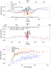 |
Fig. 17 Moving average [M/H] profile of GC late-type stars. Top panel: profile along Galactic longitude, centred on Sgr A★. Red lines denote the average over the entire FOV. Blue dashed lines are for stars at b<1 pc, that is, without stars located in the northern region of the FOV (shown as orange dot-dashed line), and the black dot-dashed line excludes stars with H − KS <1.7 mag. The average was computed with 200 stars; uncertainties are Poisson errors. The green line denotes the moving average of [M/H] of 100 stars from Feldmeier-Krause et al. (2017a, 2020). Vertical dashed lines denote the NSC Re =5 pc, and the centre at 0 pc. Middle panel: same as the top panel but including NSD data from Fritz et al. (2021), shown as purple dashed and solid orange lines with diamond symbols, and Feldmeier-Krause (2022), shown together with the Feldmeier-Krause et al. (2017a, 2020) data as green square symbols. To aid visibility, we plot error bars only every ∼20 pc. Bottom panel: profile along the observed H − KS for different regions in our FOV and averaged over 50–100 stars to account for the lower and different number of stars per field. |
6.4 Doubt on the realness of the central mean metallicity variation
Our  map indicates an increase of the mean [M/H], from roughly the inner r ≤1 pc (∼200 stars) to the surrounding region (r>1 pc, b<1 pc, –5 pc<l<5 pc, ∼650 stars), by ∼0.21 dex (see Fig. 13, middle panel and Fig. 17, top panel). The number of stars to compute
  is large, and our simulations when drawing 1000 times sub-samples of 200 stars obtain that such different values are unlikely (>2.2σ from expectations), when drawn from the same distribution. Also, the Gaussian mixture models in these regions are different. They favour a single Gaussian in the centre and a double Gaussian in the surrounding region with two rather high [M/H] values compared to other regions (e.g. north, east, or west, see Table 2).
We find a similar trend of a lower  in the inner 1 pc also in the KMOS data of Feldmeier-Krause et al. (2017a) and Feldmeier-Krause et al. (2020). We combine these two data sets, deselect foreground stars, and obtain an increase of
  by ∼0.09 dex (from r ≤1 pc to stars in the surrounding region defined as r>1 pc, b<1 pc, -4.6 pc<l<4.6 pc; 558 and 462 stars, respectively), see also green line in Fig. 17, top panel. The KMOS data do not cover the same stars as our F2 data but have some overlap (see Table B.1). The data of Feldmeier-Krause et al. (2017a), which cover only the inner r ≤1.5 pc, have the most complete sample, reaching fainter magnitudes than Feldmeier-Krause et al. (2020), which is yet deeper than our data. The absolute values of the F2
  are lower than the KMOS data by 0.2 dex and 0.08 dex. We investigate whether there may be a systematic offset between the data sets in Appendix B.1, by comparing the common stars, and find reasonable agreement, the median △[M/H] ∼0.07–0.09 dex is of the same order as the
  offset of the data sets in the surrounding regions (0.08 dex, Table B.1). The offset within the central r ≤1 pc is larger. A possible explanation is the higher completeness of the Feldmeier-Krause et al. (2017a) data, resulting in a 2.8 times larger number of stars in the inner 1 pc.
We speculate that the  decrease in the inner parsec may be a projection effect. Assuming there is a monotonous negative [M/H] gradient with increasing distance from Sgr A★, from the NSC towards the NSD, then we may observe a drop of
  towards the inner projected 1 pc, if (some of) these stars are only close in projection. In other words, their line-ofsight distance to Sgr A★ could be (on average) higher, such that their de-projected, real distance to Sgr A★ exceeds that of the stars at a projected radius 1 pc<r ≤4.5 pc. This means if we have a larger fraction of NSD or bar stars in the inner parsec region compared to the surrounding region, this could cause the low central
  . However, given the low value of
  in the central r<1 pc that is not even obtained at the NSD fields of Fritz et al. (2021), this appears unlikely.
To test the possibility of a projection effect, we compared the stellar kinematics, in particular, the line-of-sight velocity dispersion σLOS. Closer to Sgr A★, σLOS has to increase, as also the map in Fig. 14 indicates. However, the value of σLOS in the KMOS data is higher than in the F2 data, by ∼20 km s−1 (99±3 km s−1 KMOS, 76±4 km s−1 F2, central pc) to ∼8 km s−1 (82±3 km s−1 and 75±2 km s−1 in surrounding region). Thus, the stars in the KMOS data are possibly indeed closer to Sgr A★ in 3D distance than the F2 data. They are also closer in projected distance (median 0.64 pc for KMOS and 0.70 pc for F2). This may explain the differences in  between the datasets and why the F2 data have a more extreme
  drop towards the centre.
On the other hand, we cannot exclude that the low spatial resolution affects our measurements. Despite our careful extraction, the spectra of some stars may be contaminated by the flux of nearby stars. This is especially possible in the dense inner pc region and may bias the measured VLOS to the mean VLOS in the region and cause an underestimated σLOS. It may also influence our [M/H] measurements and cause the central  to decrease. In summary, we cannot exclude that the drop of the
  is (at least partially) a projection effect or caused by the low spatial resolution.
However, if the  decrease is real, it is of interest to know what could have caused it. Some mechanisms have been proposed that may affect the stellar atmosphere of red giant stars by removing their outer envelope in the central r ≲0.5 pc region. These include tidal disruption by the SMBH, interaction with a (former) jet, and collisions with dense clumps in a gas disc (e.g. MacLeod et al. 2012; Kieffer & Bogdanovic’ 2016; Amaro-Seoane et al. 2020; Zajacˇek et al. 2020; Kurfürst et al. 2024), though the first two were shown to affect mainly stars within ≲0.1 pc. Increasing the mass loss and removing the envelope of a red giant alters various properties of the star, including Teff and its brightness. The strength of the effect depends on various parameters, including the number of encounters, the distance, the surface density of the gas clouds, and the mass and radius of the star (Amaro-Seoane et al. 2020; Mastrobuono-Battisti et al. 2021). It is unclear if and how the spectrum of a red giant star changes under increased mass loss, but it was shown that red supergiant spectra alter depending on the mass loss rate (e.g. Davies & Plez 2021). It may be possible that increased mass loss in the inner r <0.5 pc affects the spectra such that they appear to have a lower [M/H].
6.5 Colour-dependent position-velocity diagram reveals NSC and NSD
We have shown the position-velocity diagram in Sect. 5, with VLOS as a function of Galactic longitude l. After removing contaminants, we compared the position-velocity diagram for stars with different values of [M/H], and we found overall good agreement for stars with sub-solar, roughly solar, or super-solar [M/H], but differences for varying observed colour H − KS.
Schultheis et al. (2021) analysed the NSD data compiled by Fritz et al. (2021). They also study the position-velocity diagram as a function of [M/H], and at the scales of their data (±1.5°∼ ±200 pc), they see significant differences. Stars at lower [M/H] show only weak rotation, and with increasing [M/H], the velocity increases, and the stars rotate faster around Sgr A★. The stars in their lowest [M/H] bin (<–0.5 dex) may even be counter-rotating and thus be remnants of accreted and disrupted star clusters or Galactic bar stars on x1 orbits. We deselected stars with extreme VLOS from our sample to decrease the bar contribution. We do not see a [M/H] dependent position-velocity curve in our NSC and NSD-dominated data. A possible reason is that our sample of stars is closer to Sgr A★ and stars with varying [M/H] are better mixed via dynamical processes. Further, the contamination fraction from the bar is significant in the data used by Schultheis et al. (2021) (∼20–62%, Sormani et al. 2022), which can cause these changes, whereas the bar contribution is much lower in our FOV (∼0 to ≲20%).
We see a dependence of the position-velocity diagram on the colour H − KS . Stars with bluer colours have a less pronounced increase of the velocity curve, increasing beyond the inner 5 pc, and they extend to larger values of l. Stars with a redder colour (in particular at H − KS =2.3–2.6 mag) have pronounced peaks of the velocity curve at ≲5 pc. As noted above, the colour can indicate line-of-sight distance dLOS. Stars with bluer colours tend to be closer to us, and stars with redder colours tend to be farther away. However, this mainly holds in regions along a small FOV, as the extinction, the main reason for the colour change, varies on scales of arcseconds. Although there is not a perfect 1:1 correlation of colour and dLOS, this, albeit noisy, relation can help one understand the colour dependence of the position-velocity diagram.
We interpret the bottom panel of Fig. 15 as follows: stars with redder colours lie deeper in the GC and therefore belong preferentially to the NSC, while bluer stars are more likely to form part of the more extended NSD. This explains the concentration of red stars around Sgr A★ and their rapidly changing velocity profile (as a function of distance from Sgr A★). The NSD stars lie at greater distances from Sgr A★, where the gravitational potential changes less rapidly, and hence, they show a flatter velocity profile. The bluest stars have the weakest rotation signal, and they are more likely to be closer and thus part of the near side of the NSD. In a future publication, we will present chemo-dynamical models of the data that will help constrain the kinematic properties of the stars in the NSC and inner NSD.
7 Conclusions
We have presented extended spectroscopic slit scan data of the GC region ranging from the NSC to the inner part of the NSD out to ±32 pc along Galactic longitude and ∼ ±1 pc along Galactic latitude. We extracted spectra of several thousand stars, predominantly red giant stars, and measured VLOS and [M/H] for more than 2500 of them.
We identified 78 hot star candidates, of which we classify 48 as likely being located in the GC. Of these, 31 are classified as hot stars for the first time. Several of the stars likely belong to the Quintuplet cluster (∼9) or the central parsec cluster (∼12). But ∼20 hot stars are rather isolated, and their origin remains an open question. Further, we detected ∼80 stars with extreme velocities (|VLOS|>150 km s−1), and we attribute these stars mainly to the Milky Way bar or tidal tails from globular clusters.
We have presented the first map of the mean [M/H] in the region beyond 1 Re of the NSC. We observed a spatial [M/H] variation with a decrease to the centre of the NSC, and we discussed the possibility that this is a projection effect caused by low spatial resolution or by high stellar mass loss in this region. We detected another  minimum where the NSD stellar density starts to dominate over the NSC at ∼10 pc (the exact location varies by a few parsecs in the east and west) and is followed by a slight increase and a flat profile in the region dominated by the NSD. We note a higher
  in the Galactic west compared to the east of the NSD.
Finally, we show the first continuous position-VLOS diagram at these scales and how it varies with [M/H] and colour H − KS . Using colour, we can separate the position-VLOS contribution of stars in the NSC and that of stars belonging to the NSD (i.e. at larger dLOS and |l|). In the future, we will use the data for detailed discrete dynamical models and to constrain the mass distribution and orbit distribution of the inner |l| <32 pc of the GC.
Acknowledgements
We thank the Gemini Observatory staff for their support during the planning and execution of the observations and advice on data reduction. We thank David Rupke for providing a general-purpose library for IFU data cubes. We also thank the anonymous referee for constructive comments and suggestions. AFK acknowledges funding from the Austrian Science Fund (FWF) [grant DOI 10.55776/ESP542]. Based on observations obtained at the international Gemini Observatory, a program of NSF NOIRLab, which is managed by the Association of Universities for Research in Astronomy (AURA) under a cooperative agreement with the U.S. National Science Foundation on behalf of the Gemini Observatory partnership: the U.S. National Science Foundation (United States), National Research Council (Canada), Agencia Nacional de Investigación y Desarrollo (Chile), Ministerio de Ciencia, Tecnología e Innovación (Argentina), Ministério da Ciência, Tecnologia, Inovações e Comunicações (Brazil), and Korea Astronomy and Space Science Institute (Republic of Korea). Data were processed using the Gemini IRAF package. IRAF is distributed by the National Optical Astronomy Observatory, which is operated by the Association of Universities for Research in Astronomy (AURA) under cooperative agreement with the National Science Foundation (Tody 1993). This research has made use of the VizieR catalogue access tool, CDS, Strasbourg, France (Ochsenbein 1996). The original description of the VizieR service was published in Ochsenbein et al. (2000). This research made use of Montage. It is funded by the National Science Foundation under Grant Number ACI-1440620, and was previously funded by the National Aeronautics and Space Administration’s Earth Science Technology Office, Computation Technologies Project, under Cooperative Agreement Number NCC5-626 between NASA and the California Institute of Technology. This research made use of NumPy (Harris et al. 2020), SciPy (Virtanen et al. 2020), matplotlib, a Python library for publication quality graphics (Hunter 2007), Astropy, a community-developed core Python package for Astronomy (Astropy Collaboration 2013, 2018, 2022). The acknowledgements were compiled using the Astronomy Acknowledgement Generator.
Appendix A Persistence removal
Our two-dimensional spectral frames of the GC contain the after-glow from the brightest stars in the acquisition images taken earlier. This is called a persistence signal. To remove the persistence, we follow a similar procedure as described in Feldmeier et al. (2014), though some changes were necessary owing to the different observing strategy, instrument, and the weaker level of persistence in our data thanks to the series of Dark exposures taken after the acquisition images. In short, we used the two acquisition images per observing block and the two-dimensional spectral frames to measure the strength of the persistence signal in the individual exposures. Then, we modelled the decrease of the persistence signal with time and used this model to subtract the persistence signal from the two-dimensional spectral frames.
We measured the persistence signal on the dark subtracted spectra; however, the persistence signal is much weaker than the flux from the sky and stars. For this reason, we required a region that is free from these sources. To subtract these sources, we first removed the distortion of the data. We measured the curvature of the stars in the two-dimensional spectrum on one of the exposures using IRAF IDENTIFY and REIDENTIFY, and we applied the transformation on both the spectra and acquisition images to create rectified files.
To measure the persistence signal and how it changes in time, we created a cutout of each rectified spectrum. We used a region with only weak sky lines, and cut out the regions along the slit (between slitlets) that stabilise the mask. Then, we subtracted the median flux along the wavelength axis, thus subtracting the sky lines. Removing the flux from stars is more complicated, as the stellar spectra have absorption lines, which leave residuals when simply subtracting the median flux along the spatial slit axis. Instead, we cut out the regions with bright stars in each spectrum. These stars are identified as follows: we computed the median flux along the slit, and fit a robust third-degree polynomial to the median flux. Then we applied 3σ clipping and measured the mean and standard deviation of the residual. We cut out regions where the residual exceeds 1 σ, which is due to bright stars. This leaves a part of the two-dimensional spectrum that is rather uniform, and the persistence signal is easily detectable. We call this two-dimensional spectrum Scut.
From the two rectified acquisition images, we created a mask M, which shows the pixels where the flux of either one of the images is higher than a certain threshold. We tried different threshold values and compared the results of the persistence model. We found little variation around values of 34 000–36 000 counts and settled on values of 34 000, 35 000, and 36 000 counts, depending on the exposure times of the images (2, 3, or 5 s). We cut the mask in the same way as the two-dimensional spectrum to obtain Mcut.
On this mask, we applied a Gaussian smoothing filter Gsmooth before subtracting it from S cut. We used MPFIT2DFUN.PRO to fit the best smoothing parameters. Those are the amplitude A, the FWHM, and an eccentricity parameter ϵ to account for an elliptical FWHM. We minimised the residual spectrum Rcut = S cut − Gsmooth ⋆ Mcut. This is done for each spectral frame in each observing block. While the FWHM and ϵ are rather stable, the amplitude A decreases with time for each series of ∼10–20 spectra, following a power law A(t) = C × t−b, where t is the UT time difference in seconds between the mean UT of the two acquisition images causing the persistence and the respective spectral frame. We then computed the value of A at the appropriate time for each two-dimensional spectral frame and used the mean values for FWHM and ϵ to apply Gsmooth on the uncut mask M, which we subtract from the un-rectified, dark subtracted spectral frames. This gives us dark and persistence-corrected two-dimensional spectral frames.
Matches with late-type star catalogues.
Appendix B Stellar parameter uncertainties
B.1 Comparison with other data
Our data overlap with the spectroscopic data analysed in Feldmeier-Krause et al. (2017a, 2020); Feldmeier-Krause (2022), and we compared our stellar parameter results. We matched the stars of our data and the literature catalogues if they are within 0″.4 of each other, their KS photometry differs by no more than 0.5 mag, and their VLOS by no more than 20 km s−1. With these three criteria, we hope to exclude most mismatches. We obtained 104, 284, and 65 matches of our data with the aforementioned papers. The stellar parameters were obtained similarly to ours, using the same code and spectral grid. However, the spectral resolution of the KMOS (VLT) instrument used in FK17, FK20, and FK22 is slightly higher (R∼4 000), and the spatial resolution is seeing limited; hence, it is less affected by contamination of nearby stars compared to our 1″ slit scan data.
We compared the median stellar parameter differences of Teff, log(g), and [M/H], and the (σ-clipped) standard deviation of the parameter difference divided by the squared sum of the statistical error (see Table B.1). The median differences are close to zero and not strongly biased. The distributions of the differences normalised with the statistical uncertainties are, however, broader than 1σ, indicating that the statistical uncertainties are underestimated. There is indeed a trend that this is more severe for the stars located in the dense and crowded NSC (FK17 and FK20) in comparison to the data at 20 pc distance (FK22), where the stellar number density is lower. We see the largest deviation for Teff (1.6σ–6σ) and log(g) (1.5σ–4.0σ), meaning that the statistical uncertainties are underestimated, whereas the uncertainties of [M/H] are reasonable (1σ–1.9σ).
From this comparison, we conclude that our statistical uncertainties for Teff and log(g) are underestimated in the central region, our statistical uncertainty for [M/H] is reasonable, and we have no strong systematic differences to the slightly higher spatial resolution data in the literature.
B.2 Systematic uncertainties
There are likely systematic uncertainties in our stellar parameter measurements, due to for example an incomplete line list used to generate the theoretical PHOENIX model grid, variation of the elemental abundances in the different stars, or imperfect interpolation of the model grid. To estimate the magnitude of these effects, we applied the same method of stellar parameter measurements on stars of the X-SHOOTER spectral library (XSL, Chen et al. 2014; Gonneau et al. 2020), and compared the results to the stellar parameter measurements of Arentsen et al. (2019), which were obtained by fitting the optical region of the XSL spectra.
To estimate systematic uncertainties, we convolved the XSL spectra to the spectral resolution of the F2 data, which is a second-degree polynomial function of wavelength. We used the average of the six slitlet regions (see Sect. 2.5). We set the same bounds for log(g) as in Feldmeier-Krause (2022). Further, we excluded peculiar stars or Carbon stars. We applied similar cuts on the fit quality (statistical uncertainties σ[M/H]<0.25 dex, σTeff <250 K, and σlog(g)<1 dex) and stellar parameter ranges ([Fe/H]A19 and [M/H] starkit >−1.3 dex, 2 800 K <Teff <6 000 K, log(g) <4.5 dex) as in Feldmeier-Krause (2022), to ensure we compare stars with similar stellar parameters as the GC data, leaving us with 232 spectra.
The mean difference to the reference values after 3σ clipping are ⟨△Teff⟩=17 K, ⟨△log(g)⟩=-0.4 dex, and ⟨△[M/H]⟩ = -0.13 dex. The standard deviation of these differences are σ△Teff =271 K, σ△ log(g)=0.9 dex, σ△[M/H]=0.32 dex. As the standard deviations are larger than the mean differences, our measurements have no strong biases, and we use the standard deviations as systematic uncertainties for our stellar parameter measurements. These values are very similar to those found by Feldmeier-Krause (2022), probably because the spectral resolution in the fit region is very similar.
For a detailed discussion of the XSL sample and its limitations to estimate systematic uncertainties for our method, see Feldmeier-Krause (2022). We also refer to Lançon et al. (2021) for a detailed comparison of the XSL SEDs with PHOENIX spectra. They found stellar parameter discrepancies for the three different X-SHOOTER arms at Teff ≲5 000 K, which may explain why our K-band results deviate from the Arentsen et al. (2019) results obtained in the X-SHOOTER VIS arm wavelength region, in particular for log(g).
Appendix C Moving average profiles of stellar parameters
We show the moving average of various photometric properties as a function of Galactic longitude l in Fig. C.1, and in addition stellar parameters Teff and log(g) in Fig. C.2. These plots correspond to Figs. 12 and 13, but they neglect any dependence on Galactic latitude b and are computed for a larger number of stars per bin (200 rather than 40), and neighbouring data points are correlated. We show the Poisson errors only for a subset of the data points, which improves visibility. We show two regions, stars from the entire FOV, and only stars at b<1 pc, that means we cut off the region in the north that covers only the central l ∼ ±8 pc.
In Fig. C.3, we show the moving average of [M/H] as a function of photometric properties for various regions, as defined in Table 2. Though we see fluctuations of  as a function of the stellar brightness KS,0, this behaviour is not identical in the regions, suggesting there is no systematic trend with stellar brightness. The bottom panel shows no consistent variation with AKS in the various regions, but rather random fluctuations of
  . The east and west regions have overall lower values of AKS , but they also overlap with the more central regions at ∼1.95–2.1 mag.
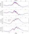 |
Fig. C.1 Moving average profile of GC late-type stars along Galactic longitude, centred on Sgr A★. Red lines denote the average over the entire FOV, and blue dashed lines for stars at b<1 pc, meaning without stars located in the northern region of the FOV. The average is computed on 200 stars, uncertainties are Poisson errors. Top panel: Observed KS band photometry; Second panel: Extinction-corrected KS,0 photometry; Third panel: Extinction in the KS band AK; Bottom panel: Observed colour H − KS . Vertical dashed lines denote the NSC Re =5 pc, and the centre at 0 pc. |
We observe a higher or at most similar value of  in the surrounding region compared to the centre and north regions irrespective of KS,0 or AKS . The same is found for the west region compared to the east. When we remove stars with [M/H] >0.5 dex, as done by Nogueras-Lara et al. (2023a), or replace those [M/H] values with a floor of 0.5 dex, the surrounding region still has higher
  than the centre, though the difference is less.
Appendix D [M/H] distributions in various regions
We show histograms of the [M/H] distribution in various regions, as listed in Table 2, and the respective Gaussian mixture models in Fig. D.1. These histograms do not include foreground stars or high-velocity stars.
Appendix E Hot star candidates with proper motion matches in the literature
In this section we present the list of hot star candidates with matches in proper motion catalogues, namely Shahzamanian et al. (2022) in Table E.1, Libralato et al. (2021) in Table E.2, and Hosek et al. (2022) in Table E.3. In Table E.5 we list all our hot star candidates.
Hot star candidates with proper motion measurement.
Hot star candidates with proper motion measurement.
Hot star candidates with proper motion measurement.
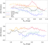 |
Fig. C.3 Moving average [M/H] profile of GC late-type stars in several regions as a function of different photometric properties. The panels show, from top to bottom, extinction corrected KS,0, extinction AKS. The regions are as defined in Table 2 and shown with colours and symbols as described in the upper panel legend. The average is computed on 50 (centre), 80 (East and West), or 100 stars (surrounding and north regions), as the number of stars varies in these regions. Uncertainties of [M/H] are Poisson errors. |
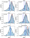 |
Fig. D.1 Gaussian mixture models of the [M/H] distribution in different regions, as detailed in Table 2. We removed likely foreground stars and high-velocity stars. The blue and red vertical lines denote the centres of the Gaussian components, and the number of stars N is noted on the top left of each panel. |
Sample of hot star candidates.
Sample of hot star candidates.
References
- Abdurro’uf, Accetta, K., Aerts, C., et al. 2022, ApJS, 259, 35 [NASA ADS] [CrossRef] [Google Scholar]
- Amaro-Seoane, P., Chen, X., Schödel, R., & Casanellas, J. 2020, MNRAS, 492, 250 [Google Scholar]
- Arentsen, A., Prugniel, P., Gonneau, A., et al. 2019, A&A, 627, A138 [NASA ADS] [CrossRef] [EDP Sciences] [Google Scholar]
- Astropy Collaboration (Robitaille, T. P., et al.) 2013, A&A, 558, A33 [NASA ADS] [CrossRef] [EDP Sciences] [Google Scholar]
- Astropy Collaboration (Price-Whelan, A. M., et al.) 2018, AJ, 156, 123 [Google Scholar]
- Astropy Collaboration (Price-Whelan, A. M., et al.) 2022, ApJ, 935, 167 [NASA ADS] [CrossRef] [Google Scholar]
- Baumgardt, H., Amaro-Seoane, P., & Schödel, R. 2018, A&A, 609, A28 [NASA ADS] [CrossRef] [EDP Sciences] [Google Scholar]
- Blum, R. D., Sellgren, K., & Depoy, D. L. 1996, AJ, 112, 1988 [Google Scholar]
- Blum, R. D., Ramírez, S. V., Sellgren, K., & Olsen, K. 2003, ApJ, 597, 323 [Google Scholar]
- Buchholz, R. M., Schödel, R., & Eckart, A. 2009, A&A, 499, 483 [NASA ADS] [CrossRef] [EDP Sciences] [Google Scholar]
- Buchner, J., Georgakakis, A., Nandra, K., et al. 2014, A&A, 564, A125 [NASA ADS] [CrossRef] [EDP Sciences] [Google Scholar]
- Cappellari, M. 2017, MNRAS, 466, 798 [Google Scholar]
- Cappellari, M., & Copin, Y. 2003, MNRAS, 342, 345 [Google Scholar]
- Chatzopoulos, S., Fritz, T. K., Gerhard, O., et al. 2015, MNRAS, 447, 948 [Google Scholar]
- Chen, Y.-P., Trager, S. C., Peletier, R. F., et al. 2014, A&A, 565, A117 [NASA ADS] [CrossRef] [EDP Sciences] [Google Scholar]
- Chen, Z., Do, T., Ghez, A. M., et al. 2023, ApJ, 944, 79 [NASA ADS] [CrossRef] [Google Scholar]
- Clark, J. S., Lohr, M. E., Najarro, F., Dong, H., & Martins, F. 2018a, A&A, 617, A65 [NASA ADS] [CrossRef] [EDP Sciences] [Google Scholar]
- Clark, J. S., Lohr, M. E., Patrick, L. R., et al. 2018b, A&A, 618, A2 [NASA ADS] [CrossRef] [EDP Sciences] [Google Scholar]
- Clark, J. S., Patrick, L. R., Najarro, F., Evans, C. J., & Lohr, M. 2021, A&A, 649, A43 [NASA ADS] [CrossRef] [EDP Sciences] [Google Scholar]
- Cotera, A. S., Simpson, J. P., Erickson, E. F., et al. 1999, ApJ, 510, 747 [Google Scholar]
- Davies, R. I. 2007, MNRAS, 375, 1099 [Google Scholar]
- Davies, B., & Plez, B. 2021, MNRAS, 508, 5757 [NASA ADS] [CrossRef] [Google Scholar]
- Do, T., Ghez, A. M., Morris, M. R., et al. 2009, ApJ, 703, 1323 [NASA ADS] [CrossRef] [Google Scholar]
- Do, T., Kerzendorf, W., Winsor, N., et al. 2015, ApJ, 809, 143 [Google Scholar]
- Do, T., Kerzendorf, W., Konopacky, Q., et al. 2018, ApJ, 855, L5 [Google Scholar]
- Dong, H., Wang, Q. D., Cotera, A., et al. 2011, MNRAS, 417, 114 [Google Scholar]
- Dong, H., Mauerhan, J., Morris, M. R., Wang, Q. D., & Cotera, A. 2015, MNRAS, 446, 842 [Google Scholar]
- Eikenberry, S. S., Elston, R., Raines, S. N., et al. 2004, SPIE Conf. Ser., 5492, 1196 [Google Scholar]
- Feldmeier-Krause, A. 2022, MNRAS, 513, 5920 [Google Scholar]
- Feldmeier, A., Neumayer, N., Seth, A., et al. 2014, A&A, 570, A2 [NASA ADS] [CrossRef] [EDP Sciences] [Google Scholar]
- Feldmeier-Krause, A., Neumayer, N., Schödel, R., et al. 2015, A&A, 584, A2 [NASA ADS] [CrossRef] [EDP Sciences] [Google Scholar]
- Feldmeier-Krause, A., Kerzendorf, W., Neumayer, N., et al. 2017a, MNRAS, 464, 194 [Google Scholar]
- Feldmeier-Krause, A., Zhu, L., Neumayer, N., et al. 2017b, MNRAS, 466, 4040 [NASA ADS] [Google Scholar]
- Feldmeier-Krause, A., Kerzendorf, W., Do, T., et al. 2020, MNRAS, 494, 396 [Google Scholar]
- Feroz, F., & Hobson, M. P. 2008, MNRAS, 384, 449 [NASA ADS] [CrossRef] [Google Scholar]
- Feroz, F., Hobson, M. P., & Bridges, M. 2009, MNRAS, 398, 1601 [NASA ADS] [CrossRef] [Google Scholar]
- Feroz, F., Hobson, M. P., Cameron, E., & Pettitt, A. N. 2019, Open J. Astrophys., 2, 10 [Google Scholar]
- Figer, D. F., McLean, I. S., & Morris, M. 1999, ApJ, 514, 202 [Google Scholar]
- Fritz, T. K., Chatzopoulos, S., Gerhard, O., et al. 2016, ApJ, 821, 44 [Google Scholar]
- Fritz, T. K., Patrick, L. R., Feldmeier-Krause, A., et al. 2021, A&A, 649, A83 [NASA ADS] [CrossRef] [EDP Sciences] [Google Scholar]
- Frogel, J. A., Stephens, A., Ramírez, S., & DePoy, D. L. 2001, AJ, 122, 1896 [Google Scholar]
- Gallego-Cano, E., Schödel, R., Nogueras-Lara, F., et al. 2020, A&A, 634, A71 [NASA ADS] [CrossRef] [EDP Sciences] [Google Scholar]
- Gallego-Cano, E., Fritz, T., Schödel, R., et al. 2024, A&A, 689, A190 [NASA ADS] [CrossRef] [EDP Sciences] [Google Scholar]
- Gonneau, A., Lyubenova, M., Lançon, A., et al. 2020, A&A, 634, A133 [NASA ADS] [CrossRef] [EDP Sciences] [Google Scholar]
- Greggio, L., & Renzini, A. 2011, Stellar Populations. A User Guide from Low to High Redshift [Google Scholar]
- Gvaramadze, V. V., & Gualandris, A. 2011, MNRAS, 410, 304 [CrossRef] [Google Scholar]
- Habibi, M., Stolte, A., & Harfst, S. 2014, A&A, 566, A6 [NASA ADS] [CrossRef] [EDP Sciences] [Google Scholar]
- Habibi, M., Gillessen, S., Martins, F., et al. 2017, ApJ, 847, 120 [Google Scholar]
- Harris, W. E. 1996, AJ, 112, 1487 [Google Scholar]
- Harris, C. R., Millman, K. J., van der Walt, S. J., et al. 2020, Nature, 585, 357 [NASA ADS] [CrossRef] [Google Scholar]
- Hosek, M. W., Do, T., Lu, J. R., et al. 2022, ApJ, 939, 68 [NASA ADS] [CrossRef] [Google Scholar]
- Hunter, J. D. 2007, Comput. Sci. Eng., 9, 90 [NASA ADS] [CrossRef] [Google Scholar]
- Husser, T. O., Wende-von Berg, S., Dreizler, S., et al. 2013, A&A, 553, A6 [NASA ADS] [CrossRef] [EDP Sciences] [Google Scholar]
- Ishchenko, M., Sobolenko, M., Kuvatova, D., Panamarev, T., & Berczik, P. 2023, A&A, 674, A70 [NASA ADS] [CrossRef] [EDP Sciences] [Google Scholar]
- Ishchenko, M., Berczik, P., Panamarev, T., et al. 2024, A&A, 689, A178 [NASA ADS] [CrossRef] [EDP Sciences] [Google Scholar]
- Kausch, W., Noll, S., Smette, A., et al. 2015, A&A, 576, A78 [NASA ADS] [CrossRef] [EDP Sciences] [Google Scholar]
- Kerzendorf, W., & Do, T. 2015, https://doi.org/10.5281/zenodo.28016 [Google Scholar]
- Kieffer, T. F., & Bogdanovic´, T. 2016, ApJ, 823, 155 [Google Scholar]
- Kleinmann, S. G., & Hall, D. N. B. 1986, ApJS, 62, 501 [NASA ADS] [CrossRef] [Google Scholar]
- Krabbe, A., Genzel, R., Drapatz, S., & Rotaciuc, V. 1991, ApJ, 382, L19 [Google Scholar]
- Kurfürst, P., ZajaCek, M., Werner, N., & Krticka, J. 2024, MNRAS, submitted [arXiv:2409.17773] [Google Scholar]
- Lançon, A., Gonneau, A., Verro, K., et al. 2021, A&A, 649, A97 [NASA ADS] [CrossRef] [EDP Sciences] [Google Scholar]
- Launhardt, R., Zylka, R., & Mezger, P. G. 2002, A&A, 384, 112 [NASA ADS] [CrossRef] [EDP Sciences] [Google Scholar]
- Libralato, M., Lennon, D. J., Bellini, A., et al. 2021, MNRAS, 500, 3213 [Google Scholar]
- Liermann, A., Hamann, W. R., & Oskinova, L. M. 2012, A&A, 540, A14 [NASA ADS] [CrossRef] [EDP Sciences] [Google Scholar]
- Lu, J. R., Ghez, A. M., Hornstein, S. D., et al. 2009, ApJ, 690, 1463 [NASA ADS] [CrossRef] [Google Scholar]
- Lu, J. R., Do, T., Ghez, A. M., et al. 2013, ApJ, 764, 155 [NASA ADS] [CrossRef] [Google Scholar]
- MacLeod, M., Guillochon, J., & Ramirez-Ruiz, E. 2012, ApJ, 757, 134 [Google Scholar]
- Martínez-Arranz, Á., Schödel, R., Nogueras-Lara, F., Hosek, M. W., & Najarro, F. 2024, A&A, 683, A3 [NASA ADS] [CrossRef] [EDP Sciences] [Google Scholar]
- Mastrobuono-Battisti, A., Church, R. P., & Davies, M. B. 2021, MNRAS, 505, 3314 [Google Scholar]
- Matsunaga, N., Kawadu, T., Nishiyama, S., et al. 2009, MNRAS, 399, 1709 [NASA ADS] [CrossRef] [Google Scholar]
- Matsunaga, N., Feast, M. W., Kawadu, T., et al. 2013, MNRAS, 429, 385 [CrossRef] [Google Scholar]
- Mauerhan, J. C., Cotera, A., Dong, H., et al. 2010a, ApJ, 725, 188 [Google Scholar]
- Mauerhan, J. C., Muno, M. P., Morris, M. R., Stolovy, S. R., & Cotera, A. 2010b, ApJ, 710, 706 [Google Scholar]
- Merritt, D. 2010, ApJ, 718, 739 [NASA ADS] [CrossRef] [Google Scholar]
- Nagayama, T., Nagashima, C., Nakajima, Y., et al. 2003, SPIE Conf. Ser., 4841, 459 [Google Scholar]
- Najarro, F., Figer, D. F., Hillier, D. J., & Kudritzki, R. P. 2004, ApJ, 611, L105 [Google Scholar]
- Nishiyama, S., & Schödel, R. 2013, A&A, 549, A57 [NASA ADS] [CrossRef] [EDP Sciences] [Google Scholar]
- Nishiyama, S., Nagata, T., Kusakabe, N., et al. 2006, ApJ, 638, 839 [Google Scholar]
- Nishiyama, S., Yasui, K., Nagata, T., et al. 2013, ApJ, 769, L28 [Google Scholar]
- Nishiyama, S., Schödel, R., Yoshikawa, T., et al. 2016, A&A, 588, A49 [NASA ADS] [CrossRef] [EDP Sciences] [Google Scholar]
- Nishiyama, S., Funamoto, N., & Schödel, R. 2023, ApJ, 951, 148 [NASA ADS] [CrossRef] [Google Scholar]
- Nogueras-Lara, F. 2024, A&A, 681, L21 [NASA ADS] [CrossRef] [EDP Sciences] [Google Scholar]
- Nogueras-Lara, F., Gallego-Calvente, A. T., Dong, H., et al. 2018, A&A, 610, A83 [NASA ADS] [CrossRef] [EDP Sciences] [Google Scholar]
- Nogueras-Lara, F., Schödel, R., Gallego-Calvente, A. T., et al. 2019, A&A, 631, A20 [NASA ADS] [CrossRef] [EDP Sciences] [Google Scholar]
- Nogueras-Lara, F., Schödel, R., Gallego-Calvente, A. T., et al. 2020a, Nat. Astron., 4, 377 [Google Scholar]
- Nogueras-Lara, F., Schödel, R., Neumayer, N., et al. 2020b, A&A, 641, A141 [EDP Sciences] [Google Scholar]
- Nogueras-Lara, F., Feldmeier-Krause, A., Schödel, R., et al. 2023a, A&A, 680, A75 [NASA ADS] [CrossRef] [EDP Sciences] [Google Scholar]
- Nogueras-Lara, F., Schultheis, M., Najarro, F., et al. 2023b, A&A, 671, L10 [NASA ADS] [CrossRef] [EDP Sciences] [Google Scholar]
- Ochsenbein, F. 1996, The VizieR database of astronomical catalogues [Google Scholar]
- Ochsenbein, F., Bauer, P., & Marcout, J. 2000, A&AS, 143, 23 [NASA ADS] [CrossRef] [EDP Sciences] [Google Scholar]
- Park, S.-M., Goodwin, S. P., & Kim, S. S. 2018, MNRAS, 478, 183 [Google Scholar]
- Paumard, T., Genzel, R., Martins, F., et al. 2006, ApJ, 643, 1011 [NASA ADS] [CrossRef] [Google Scholar]
- Pecaut, M. J., & Mamajek, E. E. 2013, ApJS, 208, 9 [Google Scholar]
- Pecaut, M. J., Mamajek, E. E., & Bubar, E. J. 2012, ApJ, 746, 154 [Google Scholar]
- Perets, H. B., Hopman, C., & Alexander, T. 2007, ApJ, 656, 709 [CrossRef] [Google Scholar]
- Pfuhl, O., Fritz, T. K., Zilka, M., et al. 2011, ApJ, 741, 108 [Google Scholar]
- Plewa, P. M. 2018, MNRAS, 476, 3974 [NASA ADS] [CrossRef] [Google Scholar]
- Portail, M., Gerhard, O., Wegg, C., & Ness, M. 2017a, MNRAS, 465, 1621 [NASA ADS] [CrossRef] [Google Scholar]
- Portail, M., Wegg, C., Gerhard, O., & Ness, M. 2017b, MNRAS, 470, 1233 [NASA ADS] [CrossRef] [Google Scholar]
- Rich, R. M., Ryde, N., Thorsbro, B., et al. 2017, AJ, 154, 239 [NASA ADS] [CrossRef] [Google Scholar]
- Rui, N. Z., Hosek, Matthew W., Lu, J. R., et al. 2019, ApJ, 877, 37 [NASA ADS] [CrossRef] [Google Scholar]
- Ryde, N., Nandakumar, G., Schultheis, M., et al. 2025, ApJ, 979, 174 [Google Scholar]
- Saito, R. K., Hempel, M., Minniti, D., et al. 2012, A&A, 537, A107 [NASA ADS] [CrossRef] [EDP Sciences] [Google Scholar]
- Schödel, R., Feldmeier, A., Kunneriath, D., et al. 2014, A&A, 566, A47 [Google Scholar]
- Schödel, R., Nogueras-Lara, F., Gallego-Cano, E., et al. 2020, A&A, 641, A102 [Google Scholar]
- Schultheis, M., Rich, R. M., Origlia, L., et al. 2019, A&A, 627, A152 [NASA ADS] [CrossRef] [EDP Sciences] [Google Scholar]
- Schultheis, M., Fritz, T. K., Nandakumar, G., et al. 2021, A&A, 650, A191 [NASA ADS] [CrossRef] [EDP Sciences] [Google Scholar]
- Shahzamanian, B., Schödel, R., Nogueras-Lara, F., et al. 2019, A&A, 632, A116 [EDP Sciences] [Google Scholar]
- Shahzamanian, B., Schödel, R., Nogueras-Lara, F., et al. 2022, A&A, 662, A11 [NASA ADS] [CrossRef] [EDP Sciences] [Google Scholar]
- Smette, A., Sana, H., Noll, S., et al. 2015, A&A, 576, A77 [NASA ADS] [CrossRef] [EDP Sciences] [Google Scholar]
- Sormani, M. C., Magorrian, J., Nogueras-Lara, F., et al. 2020, MNRAS, 499, 7 [Google Scholar]
- Sormani, M. C., Sanders, J. L., Fritz, T. K., et al. 2022, MNRAS, 512, 1857 [CrossRef] [Google Scholar]
- Støstad, M., Do, T., Murray, N., et al. 2015, ApJ, 808, 106 [CrossRef] [Google Scholar]
- Thorsbro, B., Ryde, N., Rich, R. M., et al. 2020, ApJ, 894, 26 [NASA ADS] [CrossRef] [Google Scholar]
- Tody, D. 1993, in Astronomical Society of the Pacific Conference Series, 52, Astronomical Data Analysis Software and Systems II, eds. Hanisch, R. J., Brissenden, R. J. V., & Barnes, J., 173 [NASA ADS] [Google Scholar]
- van de Ven, G., van den Bosch, R. C. E., Verolme, E. K., & de Zeeuw, P. T. 2006, A&A, 445, 513 [NASA ADS] [CrossRef] [EDP Sciences] [Google Scholar]
- van Dokkum, P. G. 2001, PASP, 113, 1420 [Google Scholar]
- Vasiliev, E. 2018, AGAMA: Action-based galaxy modeling framework, Astrophysics Source Code Library [record ascl:1805.008] [Google Scholar]
- Vasiliev, E. 2019, MNRAS, 482, 1525 [Google Scholar]
- Virtanen, P., Gommers, R., Oliphant, T. E., et al. 2020, Nat. Methods, 17, 261 [Google Scholar]
- von Fellenberg, S. D., Gillessen, S., Stadler, J., et al. 2022, ApJ, 932, L6 [NASA ADS] [CrossRef] [Google Scholar]
- Wallace, L., & Hinkle, K. 1996, ApJS, 107, 312 [NASA ADS] [CrossRef] [Google Scholar]
- Wallace, L., & Hinkle, K. 1997, ApJS, 111, 445 [NASA ADS] [CrossRef] [Google Scholar]
- Wegg, C., Gerhard, O., & Portail, M. 2015, MNRAS, 450, 4050 [NASA ADS] [CrossRef] [Google Scholar]
- Winge, C., Riffel, R. A., & Storchi-Bergmann, T. 2009, ApJS, 185, 186 [NASA ADS] [CrossRef] [Google Scholar]
- Yelda, S., Ghez, A. M., Lu, J. R., et al. 2014, ApJ, 783, 131 [Google Scholar]
- ZajaCek, M., Araudo, A., Karas, V., Czerny, B., & Eckart, A. 2020, ApJ, 903, 140 [CrossRef] [Google Scholar]
The fitted wavelength regions usually cover 1.976–2.010, 2.041–2.060, 2.192–2.21, 2.269–2.291, 2.308–2.335, 2.360–2.379, 2.412–2.440, 2.444–2.457 μm, with slight variations if it improves the fit.
All Tables
All Figures
|
Fig. 1 Spatial coverage of our observations. The data extend ∼32 pc to the Galactic east and west of Sgr A★ (marked as a red plus symbol), about 1 pc to the Galactic north and south, except for the centre region, which extends about 2 pc to the Galactic north. The image is a white light reconstructed image mosaic of our spectroscopic scans. |
| In the text | |
|
Fig. 2 Top left: reconstructed image of the data from 20 subsequent spectra. Top right: vista Variables in the Vía Láctea KS-band image cutout of the same region resampled to the pixel scale of 0.18 arcsec pixel−1. Bottom row: same as top row but convolved with a Gaussian PSF with an FWHM of 1″. The images cover ∼59″ × 22″ (2.3 × 0.9 pc). |
| In the text | |
|
Fig. 3 Example spectra of a hot star (top) and a cool star (bottom). Both spectra are normalised by their median flux, and a small offset is added to improve visibility. The vertical lines indicate several spectral features used for the analysis, labelled on the top. Both spectra have Br γ emission due to surrounding gas (the hot star has even He I emission), but only the cool star has strong Na I, Ca I and CO 2–0 absorption features, and plenty of other metal lines. The regions used to measure the spectral indices are marked by different colours in the cool star spectrum, solid lines for the feature, and dotted lines for the pseudo-continuum regions. We annotate the KS and S/N (computed using the PPXF fit residual) for each star. |
| In the text | |
|
Fig. 4 Spectral EW of Br γ, Na I, and Ca I as a function of the EW of CO 2–0. The density maps show measurements on our extracted spectra after a quality cut on the required S/N. The green x-symbols are ∼100 stars in the Wallace & Hinkle (1996, 1997) and Winge et al. (2009) spectral libraries, and the blue plus-symbols are >400 Milky Way stars from Gonneau et al. (2020). Magenta solid lines, green dashed (for Wallace & Hinkle 1996, 1997; Winge et al. 2009), and orange dot-dashed lines (Gonneau et al. 2020) show the robust mean as function of EWCO. Stars with a Br γ measurement below the dot-dashed horizontal blue line in the left panel are affected by Br γ gas emission at the centre of the NSC. |
| In the text | |
|
Fig. 5 Stellar surface density profile in the GC. Top panel: NSC profile from Chatzopoulos et al. (2015), NSD profile from Sormani et al. (2022) as a function of l. Bottom panel: fraction of the NSC and NSD density profiles, if the bar density profile is constant, and set to 20% of the NSD density profile at l = 35 pc and b = 0 pc. |
| In the text | |
|
Fig. 6 Colour-magnitude diagram of the sample with stellar parameter fit. Left panel: observed H − KS versus KS diagram for all stars with a stellar parameter fit. The vertical dashed lines enclose the stars classified as being located in the GC. Right panel: extinction corrected (H − KS )0 versus KS,0 diagram of stars with a stellar parameter fit and classified as being located in the GC. |
| In the text | |
|
Fig. 7 Proper motions of stars in the FOV. Red-coloured diamonds denote hot star candidates we classified as being located in the GC, as listed in Table E.5, and blue cross-symbols denote those hot stars we classified as non-GC stars or stars with unknown status. The black arrows indicate the proper motions of hot star candidates from Shahzamanian et al. (2022). The arrow lengths are multiplied by a factor of 3000 for better visualisation. The grey arrows are a subset (2.5%) of the Shahzamanian et al. (2022) proper motions to illustrate the distribution of proper motions in this region. Black dashed lines denote the approximate outline of our FOV, blue dashed lines the region shown in Fig. 8. The purple circle denotes Quintuplet’s tidal radius rt ∼3 pc (Rui et al. 2019), the green solid circle denotes the NSC Re = 5 pc. The x-axis and y-axis have different scales; therefore, the circles and proper motions appear elongated along the y-axis. |
| In the text | |
|
Fig. 8 Proper motions of stars in the region close to the Quintuplet cluster. Red-coloured diamonds denote hot star candidates we classified as being located in the GC, and blue cross-symbols denote those stars we classified as non-GC stars or stars with unknown status. The red arrows indicate the proper motions of our hot star candidates from Hosek et al. (2022). The arrow lengths are multiplied by a factor of 3000 for better visualisation. The grey arrows are a subset of the Hosek et al. (2022) proper motions, showing 33% of the stars with more than 80% cluster probability. Black dashed lines denote the approximate outline of our FOV. The dashed purple circle denotes Quintuplet’s core radius rc, the solid purple circle its tidal radius rt (adopted from Rui et al. 2019), and the purple arrow pointing at the centre denotes the direction of the orbit of Quintuplet (Fig. 6 in Hosek et al. 2022). Green coloured squares denote spectroscopic hot Quintuplet stars from Clark et al. (2018a), magenta triangles are Paschen α candidates from Dong et al. (2011). |
| In the text | |
|
Fig. 9 Density of late-type GC stars with stellar parameter measurements, as a function of Galactic longitude and Galactic latitude, centred on Sgr A★. We have the largest density in the centre of our field, where the stellar density is also the highest. The higher density in the inner 5 pc east of Sgr A★ compared to inner 5 pc west of Sgr A★ is likely caused by the lower extinction of the east region (see also Fig. 12, bottom panel), and is already visible in the photometric catalogue. We note that the vertical axis is stretched relative to the horizontal axis of the plot to improve visibility. |
| In the text | |
|
Fig. 10 Stellar parameter distributions of GC stars. From left to right panel, effective temperature Teff, overall metallicity [M/H], and surface gravity log(g). We denote the mean, median, and standard deviation of the distributions on each panel, and we show the mean statistical and total uncertainty with a cross and diamond symbol. |
| In the text | |
|
Fig. 11 Position-velocity plot of GC late-type stars along Galactic longitude, centred on Sgr A★. Each diamond symbol denotes a star, and green x-symbols denote stars that we consider high-velocity stars. The red line denotes the moving average VLOS of 150 stars, the blue lines denote the moving robust σr × 2.5, which is close to our cuts to classify high-velocity stars, shown as dashed horizontal lines. |
| In the text | |
|
Fig. 12 Mean photometric properties in different Voronoi bins: KS,0 (top), H − KS (middle), and AKS ,0 (bottom). The mean KS,0 indicates that the stars in the central region are slightly fainter than stars in the outer regions, especially in the west. The stars in the centre are slightly redder (higher mean H − KS ), and in this region, the extinction AKS is higher. High-velocity stars and foreground stars were excluded. Each bin contains ∼40 stars. |
| In the text | |
|
Fig. 13 Mean effective temperature Teff, overall metallicity [M/H], and surface gravity log(g). The regions with fainter stars in Fig. 12 (top panel) have higher Teff and log(g), as expected. High-velocity stars and foreground stars were excluded. Each bin contains ∼40 stars. |
| In the text | |
|
Fig. 14 Mean line-of-sight velocity VLOS (top) and velocity dispersion σLOS (bottom) in bins of ∼40 stars. High-velocity stars and foreground stars were excluded. |
| In the text | |
|
Fig. 15 Binned position–velocity plots of GC late-type stars after removing high-velocity stars, along Galactic longitude, centred on Sgr A★. Top panel: position–velocity curves for different [M/H] bins (moving average of 100 stars). Different colours and lines denote the different [M/H] selection (see figure legend). Bottom panel: same as top panel but applying bins in H − KS . |
| In the text | |
|
Fig. 16 Spatial distribution and 3D motions of high-velocity stars in the FOV. The blue-to-red coloured symbols denote high-velocity stars, colourcoded by their VLOS. The arrows denote the direction of their proper motion from Shahzamanian et al. (2022), but the arrow length is multiplied by a factor of 3000 for better visualisation. The grey arrows are a subset (2.5%) of the Shahzamanian et al. (2022) proper motions to illustrate the distribution of proper motions in this region. Black dashed lines denote the approximate outline of our FOV. The x-axis and y-axis have different scales; therefore, proper motions along the y-axis appear larger. The green circle denotes 1 Re = 5 pc of the NSC. |
| In the text | |
|
Fig. 17 Moving average [M/H] profile of GC late-type stars. Top panel: profile along Galactic longitude, centred on Sgr A★. Red lines denote the average over the entire FOV. Blue dashed lines are for stars at b<1 pc, that is, without stars located in the northern region of the FOV (shown as orange dot-dashed line), and the black dot-dashed line excludes stars with H − KS <1.7 mag. The average was computed with 200 stars; uncertainties are Poisson errors. The green line denotes the moving average of [M/H] of 100 stars from Feldmeier-Krause et al. (2017a, 2020). Vertical dashed lines denote the NSC Re =5 pc, and the centre at 0 pc. Middle panel: same as the top panel but including NSD data from Fritz et al. (2021), shown as purple dashed and solid orange lines with diamond symbols, and Feldmeier-Krause (2022), shown together with the Feldmeier-Krause et al. (2017a, 2020) data as green square symbols. To aid visibility, we plot error bars only every ∼20 pc. Bottom panel: profile along the observed H − KS for different regions in our FOV and averaged over 50–100 stars to account for the lower and different number of stars per field. |
| In the text | |
|
Fig. C.1 Moving average profile of GC late-type stars along Galactic longitude, centred on Sgr A★. Red lines denote the average over the entire FOV, and blue dashed lines for stars at b<1 pc, meaning without stars located in the northern region of the FOV. The average is computed on 200 stars, uncertainties are Poisson errors. Top panel: Observed KS band photometry; Second panel: Extinction-corrected KS,0 photometry; Third panel: Extinction in the KS band AK; Bottom panel: Observed colour H − KS . Vertical dashed lines denote the NSC Re =5 pc, and the centre at 0 pc. |
| In the text | |
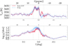 |
Fig. C.2 Same as Fig. C.1 but for stellar parameters. Top panel: Teff. Bottom panel: log(g). |
| In the text | |
|
Fig. C.3 Moving average [M/H] profile of GC late-type stars in several regions as a function of different photometric properties. The panels show, from top to bottom, extinction corrected KS,0, extinction AKS. The regions are as defined in Table 2 and shown with colours and symbols as described in the upper panel legend. The average is computed on 50 (centre), 80 (East and West), or 100 stars (surrounding and north regions), as the number of stars varies in these regions. Uncertainties of [M/H] are Poisson errors. |
| In the text | |
|
Fig. D.1 Gaussian mixture models of the [M/H] distribution in different regions, as detailed in Table 2. We removed likely foreground stars and high-velocity stars. The blue and red vertical lines denote the centres of the Gaussian components, and the number of stars N is noted on the top left of each panel. |
| In the text | |
Current usage metrics show cumulative count of Article Views (full-text article views including HTML views, PDF and ePub downloads, according to the available data) and Abstracts Views on Vision4Press platform.
Data correspond to usage on the plateform after 2015. The current usage metrics is available 48-96 hours after online publication and is updated daily on week days.
Initial download of the metrics may take a while.