| Issue |
A&A
Volume 646, February 2021
|
|
|---|---|---|
| Article Number | A3 | |
| Number of page(s) | 17 | |
| Section | Interstellar and circumstellar matter | |
| DOI | https://doi.org/10.1051/0004-6361/202039387 | |
| Published online | 02 February 2021 | |
Chemically tracing the water snowline in protoplanetary disks with HCO+
1
Leiden Observatory, Leiden University,
PO box 9513,
2300 RA Leiden, The Netherlands
e-mail: This email address is being protected from spambots. You need JavaScript enabled to view it.
2
University of Michigan, Department of Astronomy, 1085 S. University,
Ann Arbor,
MI 48109, USA
3
Anton Pannekoek Institute for Astronomy, University of Amsterdam,
Science Park 904,
1090 GE Amsterdam, The Netherlands
4
National Radio Astronomy Observatory,
520 Edgemont Road,
Charlottesville,
VA 22903-2475, USA
5
Max-Planck-Institut für Extraterrestrische Physik,
Giessenbachstrasse 1,
85748 Garching, Germany
Received:
10
September
2020
Accepted:
22
November
2020
Abstract
Context. The formation of planets is expected to be enhanced around snowlines in protoplanetary disks, in particular around the water snowline. Moreover, freeze-out of abundant volatile species in disks alters the chemical composition of the planet-forming material. However, the close proximity of the water snowline to the host star combined with the difficulty of observing water from Earth makes a direct detection of the water snowline in protoplanetary disks challenging. HCO+ is a promising alternative tracer of the water snowline. The destruction of HCO+ is dominated by gas-phase water, leading to an enhancement in the HCO+ abundance once water is frozen out.
Aims. Following earlier observed correlations between water and H13CO+ emission in a protostellar envelope, the aim of this research is to investigate the validity of HCO+ and the optically thin isotopologue H13CO+ as tracers of the water snowline in protoplanetary disks and the required sensitivity and resolution to observationally confirm this.
Methods. A typical Herbig Ae disk structure is assumed, and its temperature structure is modelled with the thermochemical code DALI. Two small chemical networks are then used and compared to predict the HCO+ abundance in the disk: one without water and one including water. Subsequently, the corresponding emission profiles are modelled for the J = 2−1 transition of H13CO+ and HCO+, which provides the best balance between brightness and the optical depth effects of the continuum emission and is less affected by blending with complex molecules. Models are then compared with archival ALMA data.
Results. The HCO+ abundance jumps by two orders of magnitude over a radial range of 2 AU outside the water snowline, which in our model is located at 4.5 AU. We find that the emission of H13CO+ and HCO+ is ring-shaped due to three effects: destruction of HCO+ by gas-phase water, continuum optical depth, and molecular excitation effects. Comparing the radial emission profiles for J = 2−1 convolved with a 0′′.05 beam reveals that the presence of gas-phase water causes an additional drop of only ~13 and 24% in the centre of the disk for H13CO+ and HCO+, respectively. For the much more luminous outbursting source V883 Ori, our models predict that the effects of dust and molecular excitation do not limit HCO+ as a snowline tracer if the snowline is located at radii larger than ~40 AU. Our analysis of recent archival ALMA band 6 observations of the J = 3−2 transition of HCO+ is consistent with the water snowline being located around 100 AU, further out than was previously estimated from an intensity break in the continuum emission.
Conclusions. The HCO+ abundance drops steeply around the water snowline, when water desorbs in the inner disk, but continuum optical depth and molecular excitation effects conceal the drop in HCO+ emission due to the water snowline. Therefore, locating the water snowline with HCO+ observations in disks around Herbig Ae stars is very difficult, but it is possible for disks around outbursting stars such as V883 Ori, where the snowline has moved outwards.
Key words: astrochemistry / protoplanetary disks / ISM: molecules / submillimeter: planetary systems
© ESO 2021
1 Introduction
High resolution observations of protoplanetary disks show that many of them have rings, gaps, and other substructures (e.g. Andrews et al. 2010; van der Marel et al. 2015; Fedele et al. 2017; Huang et al. 2018; Long et al. 2018; and Andrews 2020 for a review). Different explanations have been proposed for these substructures, such as planets (e.g. Bryden et al. 1999; Zhu et al. 2014; Dong et al. 2018) and snowlines (e.g. Banzatti et al. 2015; Zhang et al. 2015; Okuzumi et al. 2016). A snowline is the midplane radius in a protoplanetary disk where 50% of a volatile is in the gas phase and 50% is frozen out onto the dust grains. These snowlines are related to planet formation because dust properties change around the snowlines of the major volatiles: H2O, CO, and CO2 (Pinilla et al. 2017). Even though water ice mantles may not always aid dust coagulation by collisions (Kimura et al. 2020), the sublimation, condensation, and diffusion of gas-phase water enhances the surface density around the water snowline, aiding planet formation and potentially triggering the streaming instability (e.g. Stevenson & Lunine 1988; Drążkowska & Alibert 2017; Schoonenberg & Ormel 2017).
Snowlines do not only influence the formation of planets. They are also key in setting their chemical composition. The sequential freeze-out of the major volatile species changes the bulk chemical composition, often measured as the C/O ratio, of the planet-forming material, with the ice becoming more oxygen-rich than the gas (Öberg et al. 2011; Eistrup et al. 2016, 2018). The water snowline is of particular importance as water is crucial for the development of life.
Knowledge of the water snowline location is thus essential for the understanding of planet formation and composition. Yet observing water snowlines is challenging because their expected location is only a few AU from the host star for T Tauri disks (Harsono et al. 2015) and ~10 AU for disks around more luminous Herbig Ae stars. Therefore, observations with very high spatial resolution are necessary. On top of that, observing water snowlines directly from the ground by observing gas-phase water in protoplanetary disks is challenging because of the absorption of water in the Earth’s atmosphere. The only detections of water in protoplanetary disks probe either the innermost hot regions of the disk (≲ 5 AU; e.g. Carr & Najita 2008; Salyk et al. 2008; Mandell et al. 2012) or the cold outer disk with space-based telescopes, analysing multiple water lines (Hogerheijde et al. 2011; Zhang et al. 2013; Blevins et al. 2016; Salinas et al. 2016; Du et al. 2017) or have used both ground-based and space-based telescopes (Banzatti et al. 2017; Salyk et al. 2019). Targeting less abundant isotopologues of water, for example H O, reduces the atmospheric absorption, but detecting these molecules at a significant signal-to-noise ratio (S/N) greatly increases the required observing time (e.g. Notsu et al. 2019). Space-based telescopes circumvent this problem but for now lack the spatial resolution to resolve the water snowline.
Chemical tracers provide an alternative way of locating snowlines. Some detections of molecules in disks show ring-shaped emission even if the density of the disk is smooth. One example of such a molecule is CN, which is enhanced if a strong UV field is present (e.g. van Zadelhoff et al. 2003; Teague et al. 2016; Cazzoletti et al. 2018). Other examples are molecules that trace snowlines. Chemical imaging has been used to locate the CO snowline in the disks around TW Hya and HD 163296 using N2 H+ and DCO+ (Mathews et al. 2013; Qi et al. 2013, 2015, 2019). Both tracers show ring-shaped emission but detailed chemical modelling is needed to infer the location of the CO snowline from these observations (Aikawa et al. 2015; van ’t Hoff et al. 2017; Carney et al. 2018).
Water can be traced chemically using the HCO+ ion, which is destroyed by gas-phase water (Phillips et al. 1992; Bergin et al. 1998):
 (1)
(1)
Based on this reaction, HCO+ is expected to be abundant when water is frozen out onto the grains, and HCO+ is expected to be depleted when water is in the gas phase. This anti-correlation between water and HCO+ has been verified observationally by the optically thin isotopologue H13 CO+ and an isotopologue of water H O in a protostellar envelope (van ’t Hoff et al. 2018a). Due to the high luminosity of young stellar objects at this early stage, the snowline is located further away from the star than in protoplanetary disks (Visser & Bergin 2012; Jørgensen et al. 2013; Vorobyov et al. 2013; Visser et al. 2015; Cieza et al. 2016; Hsieh et al. 2019). Similarly, the higher luminosity of Herbig Ae stars compared to T Tauri stars increases the temperature in the protoplanetary disks around them, which locates the water snowline further out in disks around the former type. Therefore, we focus on protoplanetary disks around Herbig Ae stars in this work.
The aim of this paper is to investigate HCO+ as a tracer of the water snowline in protoplanetary disks. Compared to protostellar envelopes, the 2D temperature and density structure of disks complicates matters. First, the location of the water snowline in protoplanetary disks around Herbig Ae stars is expected around 10 AU, in contrast to ≳100 AU in protostellar envelopes. Second, the higher column density in disks increases the optical depth of the continuum and line emission. This complicates locating the water snowline as emission from HCO+ can be absorbed by dust particles, mimicking the effect of depletion due to gas-phase water on the HCO+ emission. Finally, the HCO+ emission can also be ring-shaped when the J-level population of the low levels, which can be observed with ALMA, decreases towards the centre of the star due to the increase in temperature and density in the inner disk. This also mimics the effect of gas-phase water on the HCO+ emission.
The validity of HCO+ as a tracer of the water snowline in protoplanetary disks is investigated by modelling the physical and chemical structure of a disk around a typical Herbig Ae star with a luminosity of 36 L⊙ as described in Sect. 2. The predicted abundance structure of HCO+ is presented in Sect. 3.1, and the corresponding emission profiles of HCO+ and H13 CO+ are described in Sects. 3.2 and 3.3. Archival ALMA observations of H13 CO+ and HCO+ in the outbursting source V883 Ori are discussed in Sect. 4. Finally, we conclude in Sect. 5 that it is difficult to use HCO+ as a tracer of the water snowline in disks around Herbig Ae stars, but that it is possible for outbursting sources such as V883 Ori.
2 Protoplanetary disk model
The HCO+ and H13 CO+ radial emission profiles were modelled in several steps. First, a density structure for a typical disk around a Herbig Ae star was assumed. Second, the gas temperature was calculated using the thermochemical code DALI (Bruderer et al. 2009, 2012; Bruderer 2013). The gas density and gas temperature were then used as input for two chemical models, one without water and one with water, that predict the HCO+ abundance in the disk. These abundance profiles together with the density and temperature structure of the disk were used to compute the HCO+ and H13 CO+ emission profiles with DALI.
2.1 Disk structure
The density structure of the disk was modelled with the thermochemical code DALI following the approach of Andrews et al. (2011). This approach is based on the self-similar solution for a viscously evolving disk, where the gas surface density of the disk outside the dust sublimation radius follows a power law with an exponential taper (Lynden-Bell & Pringle 1974; Hartmann et al. 1998):
![Mathematical equation: \begin{align*} \Sigma_{\mathrm{gas}} (R)\,{=}\,\Sigma_{\mathrm{c}} \left (\frac{R}{R_{\mathrm{c}}} \right)^{-\gamma} \exp \left [-\left (\frac{R}{R_{\mathrm{c}}}\right)^{2-\gamma} \right ], \end{align*}](/articles/aa/full_html/2021/02/aa39387-20/aa39387-20-eq4.png) (2)
(2)
with Σc the gas surface density at the characteristic radius Rc, and γ the power law index. A sublimation radius of Rsubl = 0.05 AU was assumed. Inside this radius, the number density was set to 7 × 102 cm−3. An overview of all parameters used for the density and temperature structure can be found in Table 1.
The gas follows a Gaussian distribution in the vertical direction, where the temperature was calculated explicitly at each location in the disk. The scale height of the gas was set by the flaring index ψ and the characteristic scale height hc at Rc,
 (3)
(3)
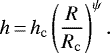
The resulting gas density of our model is shown in the top panel of Fig. 1.
The dust surface density was modelled with DALI by scaling the gas surface density with the disk-averaged gas-to-dust mass ratio, Δgas∕dust, which was set to the ISM value of 100. The vertical structure of the dust was modelled using two populations of dust grains following the approach of D’Alessio et al. (2006). Small grains with sizes between 5 nm and 1 μm are well mixed with the gas and therefore both follow the same vertical structure. Large grains with sizes from 5 nm to 1 mm are settled to the disk midplane. This was modelled by reducing the scale height of the large grains with a factor of χ < 1. The fraction of the dust mass in large grains was controlled by fls and the size distribution of both grain populations was assumed to be proportional to a−3.5, with a the size of the grains (MRN distribution, Mathis et al. 1977).
The gas temperature needed to be computed separately as the abundances of the molecules that act as coolants of the gas in the disk affected the gas temperature, which in turn affected the chemistry. Therefore, DALI solves for the gas temperature by iterating over the chemistry and heating by the photoelectric effect and the cooling by molecules in the gas. The dust temperature was computed using Monte Carlo continuum radiative transfer. The gas and dust temperature calculated by DALI are shown in the middle and bottom panel of Fig. 1. The gas temperature exceeds the dust temperature in the surface layers only, whereas the gas and dust temperatures are equal in deeper layers of the disk.
DALI model parameters for the disk around a typical Herbig Ae star.
 |
Fig. 1 Assumed gas density (top) and computed gas and dust temperature (middle and bottom panels) in the DALI model for a typical disk around a Herbig Ae star with a luminosity of 36 L⊙. Only the region where n(gas) > 106 cm-3 is shown. The position of the star is indicated with the symbol of a black star and the Tdust = 150 K line, approximating the water snow surface, is indicated with the solid grey line. |
2.2 Chemical models
The HCO+ abundance with respect to the total number of hydrogen atoms in the disk was modelled with a small chemical network, which was solved time-dependently up to 1 Myr with the python function odeint1. This allowed us to more easily study the effect of different parameters than with a computationally more expensive full chemical model. The HCO+ abundance in protoplanetary disks is mainly controlled by three reactions. The main formation route of HCO+ involves gas-phase CO:
Reaction coefficients of the reactions used in this paper.
 (4)
(4)
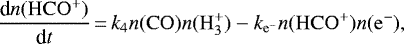
Here, H is producedby cosmic ray ionisation of molecular hydrogen at a rate of ζcr. On the other hand, HCO+ is destroyed by gas-phase water (Eq. (1)) and by dissociative recombination with an electron:
 (5)
(5)
Therefore, a jump in the HCO+ abundance around the water snowline is expected if electrons are not the dominant destruction mechanism of HCO+.
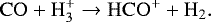
To investigate the relationship between HCO+ and H2O, two small chemical networks were used. The first network, network no water (NW), is shown in the dashed box in Fig. 2. This network includes three reactions to model the ionisation in the disk (reactions ζcr, k2, and k3 in Table 2), and two reactions to model the HCO+ abundance in the absence of gas-phase water (reactions k4 and  (Eqs. (4) and (5)) in Table 2). As reaction
  (Eq. (1)) is not included in this network, HCO+ is not expected to trace the water snowline in network NW. Therefore, this network serves as a baseline to quantify the effect of the gas-phase water on theHCO+ abundance. The second network, network water (W), is shown in the solid box in Fig. 2 and contains all reactions present in Table 2. Network W includes those in network NW together with reactions to model the effect of water on the HCO+ abundance. The most important reaction for our study is indicated in red in Fig. 2 and is the destruction of HCO+ by gas-phase water (reaction
  or Eq. (1)). Therefore, HCO+ is expected to trace the water snowline in network W. The other reactions present in network W include the freeze-out and desorption of water (reactions kf and kd), and the formation and destruction of gas-phase water from and to H3 O+ (reactions k7 and k8). The equations for the freeze-out and desorption rates of water can be found in Appendix A.
Initially, the abundance of all gas- and ice-phase species were set to 0 except for the abundance of gas-phase CO, which was set to 10−4 both in network NW and W, and the abundance of gas-phase water in network W, which was set to 3.8 × 10⁻⁷, appropriate for a dark cold cloud (McElroy et al. 2013), see also Table B.1. The rate coefficient for the freeze-out of water depends on multiple parameters, including the number density and size of the grains. Therefore, we assumed in chemical network NW and W a typical grain number density of 10−12 × n(H2) and a grain size of 0.1 μm, which set the surface area available for chemistry on grains. Assuming a single grains size for the chemistry is an approximation, but the effect of grain growth in disks, which decreases this area, is cancelled by the dust settling in disks, which increases this area as there is more dust available for chemistry in the midplane (Eistrup et al. 2016). Finally, the H13 CO+ abundance was taken to be a factor of 70 smaller than the abundance of HCO+, corresponding to the typical 12 C/13C isotope ratio (Milam et al. 2005).
 |
Fig. 2 Schematic view of chemical networks NW (no water) and W (water) used to predict the abundance of HCO+. The first network, network NW, only includes the reactions enclosed in the dashed box. The second network, network W, includes all reactions present in the figure. The destruction of HCO+ by gas-phase water is indicated with the thick red arrow. |
2.3 Radiative transfer
Predictions for multiple transitions of HCO+ and H13 CO+ were made using the ray tracer in DALI, where the outputs of the chemical networks discussed in Sect. 2.2 were used to set the abundance, and both line and continuum optical depth are included. The line radiative transfer did not assume LTE. Instead, the excitation was calculated explicitly, where we used the collisional rate coefficients in the LAMDA database (Botschwina et al. 1993; Flower 1999; Schöier et al. 2005).
Furthermore, the disk was assumed to be located at a distance of 100 pc and the inclination was taken to be 38°. Changing the inclination did not significantly change our results. The radial emission profiles were taken to be along the semi-major axis of the disk. The focus in the paper is on the J = 2−1 transition at 178.375 and 173.507 GHz for HCO+ and H13 CO+, respectively, because this transition provided the best balance between the brightness of the line and the effects of the continuum optical depth. Moreover, the higher transitions could be blended with emission from complex organic molecules. Predictions for the weaker J = 1−0 transition, as well as the brighter J = 3−2 and J = 4−3 transitions, that are more affected by the optical depth of the continuum emission and emission from complex organic molecules, can be found in Appendix C. To mimic high resolution ALMA observations, the emission was convolved with a 0′′.05 beam, unless denoted otherwise.
3 Modelling results
3.1 Chemistry
The predicted abundances of HCO+ by chemical networks NW and W are presented in Fig. 3. The water snow surface in network W is computed as the surface where 50% of the total water abundance is in the gas-phase and 50% is frozen-out onto the grains, and is indicated by the black line. In this model, the water snowline, the midplane location where water freezes-out, is located at 4.5 AU. The two networks predict very similar HCO+ abundances outside and below the water snow surface. This is due to the fact that water is frozen out outside the water snow surface in network W, hence there is very little gas-phase water available for the destruction of HCO+. In network W, the HCO+ abundance drops inside the snowline, and is in general at least two orders of magnitude lower than in network NW. Up to 2 AU outside the water snowline HCO+ is still efficiently destroyed by the small amount of water that is present in the gas-phase. Similar effects were found for N2 H+ and CO (Aikawa et al. 2015; van ’t Hoff et al. 2017). Therefore, HCO+ is efficiently destroyed by gas-phase water, and is thus a good chemical tracer of the water snowline.
The morphology of the HCO+ distribution predicted by chemical network W is similar to the morphology predicted by full chemical networks (Walsh et al. 2012, 2013; Agúndez et al. 2018). Chemical network W agrees with the full chemical networks quantitatively inside the water snowline, where all studies predict a low HCO+ abundance of ≲10−14. Moreover, the full networks and network W all show a jump of at least one order of magnitude in the HCO+ abundance over a radial range of 5 AU outside the water snowline. In addition, these models predict a layer starting at z∕r ~ 0.1 where the HCO+ abundance reaches a high abundance of 10−6−10−7 (Walsh et al. 2012, 2013, and Agúndez et al. 2018). Yet, this layer is not expected to contribute much to the column density and emission of HCO+ because the gas densities are low in this layer of the disk. The midplane abundances at 10 AU are ~ 10−12 in the full networks and 10−11 in network W, though the gradient in the HCO+ abundance is very steep between the water snowline at 4.5 AU and a radius of 10 AU in network W complicating comparison. An HCO+ abundance of 10−12 is reached at 7 AU. The HCO+ abundance at 100 AU lies within the range of HCO+ abundances predicted by the full chemical models. Our small network is thus suited to study HCO+ as a tracer of the water snowline.
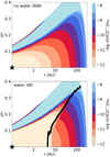 |
Fig. 3 HCO+ abundance calculated using chemical network NW (top) and network W (bottom). The water snow surface is marked with the black line in the bottom panel. The position of the star in indicated with the symbol of a black star. |
3.1.1 Water versus electrons
HCO+ only acts as a tracer of the water snowline if the destruction of HCO+ by electrons is not dominant over the destruction by gas-phase water. The dissociative recombination of HCO+ with an electron is included in both chemical networks. The rates of the reactions in Eq. (1) and Eq. (5),  and
and  , respectively, are given by:

Using Table 2, the ratio of these reaction rates is given by:
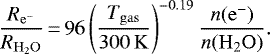 (8)
(8)
Therefore, gas-phase water is the dominant destruction mechanism of HCO+ if the number density of gas-phase water is about two orders of magnitude larger than the number density of electrons.
Figure 4 shows this ratio for chemical network W. The region where electrons are the dominant destruction mechanism ( ) is indicated in red and the region where water is dominant (
 ) is indicated in blue. The first region exists mostly outside the water snow surface as water is frozen out. The latter region exists mostly inside and above the water snow surface because there is plenty of water to destroy HCO+ in these regions. Therefore, HCO+ is a good chemical tracer of the water snowline even though electrons are its dominant destruction mechanism in most of the disk.
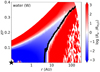 |
Fig. 4 Relative reaction rates of HCO+ destruction by electrons ( |


3.1.2 Effect of the CO, H2O abundance, and cosmic ray ionisation rate on the HCO+ abundance
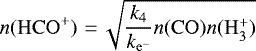
In this section we investigate the choice of initial conditions for chemical network W listed in Table B.1. The HCO+ abundance outside the water snow surface in chemical network W can be approximated analytically (for details see Appendix B.1):
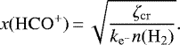 (9)
(9)
Based on this equation, it is expected that the abundance of HCO+ scales as thesquare root of the cosmic ray ionisation rate in the disk region outside the water snowline. This analytical prediction is consistent with the predictions made by the numerical solution to chemical network W (top left panel in Fig. B.1), where the HCO+ column density decreases by one order of magnitude if the cosmic ray ionisation rate decreases by two orders of magnitude.
Furthermore, the HCO+ abundance is expected to be independent of the initial CO and H2 O abundance outside the water snow surface based on the analytical approximation. This is in line with the predictions by the numerical solution to chemical network W (see HCO+ column density in Fig. B.1). The only major difference between the analytical approximation and the numerical solution occurs inside the water snowline. If the initial abundance of gas-phase water increases up to ~ 5 × 10⁻⁵, as expected for water ice in cold clouds, the column density of HCO+ inside the water snowline decreases. This is because the higher abundance of gas-phase water destroys more HCO+. There is no significant effect on the HCO+ column density outside the water snowline as all water is frozen out in that region of the disk. In summary, HCO+ shows a steep jump in its column density around the water snowline for all initial conditions discussed in this section. Therefore, the results in the following sections do not depend critically on the choice of initial conditions. Further details on the initial conditions can be found in Appendix B.2.
3.2 HCO+ and H13 CO+ emission
Observations of gas in disks do not directly trace the local abundances, only the line emission that is closely related to the column densities if the line emission is optically thin. The column densities of HCO+ and the predicted radial emission profiles of HCO+ and H13 CO+ in network NW and W are shown in Fig. 5. Similar to the abundance plots of HCO+, the total HCO+ column density jumps by a factor of ~230 over a radial range of 3 AU outside the water snowline in network W (solid blue line, top panel). Therefore, the HCO+ column density shows a clear dependence on the presence of gas-phase water, and the high HCO+ abundance in the surface layers of the disk does not contribute much to the column density.
On the other hand, the shapes of the radial emission profiles of the HCO+ J = 2−1 transition are very similar for networks NW and W, and the profiles peak at the same radius outside the water snowline (solid lines, middle panel). This is different from the HCO+ column densities, where only network W predicts the HCO+ column density to peak outside the water snowline. The drop in the column density around the water snowline translates into a relative maximum difference of only 24% between the radial emission profiles of the J = 2−1 transition of HCO+. This maximum relative difference is defined as the maximum difference between the flux predicted by network NW and W compared to the maximum flux predicted by network W, and is typically located at the water snowline.
HCO+ is more abundant than H13 CO+, hence H13 CO+ emission is expected to be optically thin, whereas the HCO+ emission is optically thick. To test if this affects the ability to trace the water snowline, we predict emission from the less abundant isotopologue H13 CO+. The radial emission profiles of H13 CO+ for both chemical networks are shown in the bottom panel of Fig. 5. Qualitatively the profiles are similar to the predicted emission for HCO+. Though the expected flux is about 39 times lower for H13 CO+ than for HCO+. This difference in flux is less than a factor of 70, which indicates that the HCO+ emission is indeed at least partially optically thick. The relative maximum difference between chemical network NW and W is 13% for H13 CO+, which is almost half of the corresponding number for HCO+. So the effect of the water snowline is also seen in the emission of the optically thin H13 CO+, but even less prominently than in HCO+. This is because H13 CO+ emits from a lower layer in the disk due to its lower optical depth. Therefore, more dust is present above the layer where H13 CO+ emits, hence the effect of dust is larger for H13 CO+ than for HCO+.
These models show very similar radial emission profiles predicted for network NW and W with only a small difference in flux. Both networks predict ring shaped emission, regardless of the presence of the water snowline. This decrease in line flux towards the centre of the disk can have different origins. The first one is a decrease in the abundance of the observed molecule, discussed in the previous section, which is the effect we aim to observe. However, the optical depth of the continuum emission and molecular excitation effects can change the emission as well, potentially obscuring the effect we aim to trace.
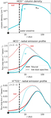 |
Fig. 5 HCO+ column density and emission in a disk around a typical Herbig Ae star. Top panel: total HCO+ column densities. Middle and bottom panels: HCO+ J = 2− 1 radial emission profiles and H13CO+ J = 2− 1 radial emission profiles along the major axis predicted for chemical network NW (red) and chemical network W (light blue). The dotted lines refer to a model with very low dust opacities to lower the effects of continuum optical depth (see Sect. 3.2.1). The water snowline is indicated with the dashed black line. The radial emission profiles are convolved with a 0′′.05 beam. |
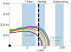 |
Fig. 6 τdust = 1 surface at the wavelength of the HCO+ J = 1− 0 transition (3.4 mm, brown), J = 2−1 (1.7 mm, orange), J = 3−2 (1.2 mm, green), and J = 4−3 (0.84 mm, purple). The radial range where the water snowline is expected for various types of sources is highlighted with the blue background. The water snowline in the model for a typical Herbig Ae disk is indicated with the dashed black line. |
3.2.1 Continuum optical depth
The continuum affects the line intensity when the optical depth of the continuum emission is larger than the optical depth of the line or when both are optically thick (Isella et al. 2016). To investigate the effect of the continuum emission, the J = 2−1 transition of HCO+ and H13 CO+ was ray traced in a disk model where the dust opacities (dust mass absorption coefficients κν) were divided by a factor of 1010, to cancel the effect of dust on the HCO+ emission compared to the typical Herbig Ae disk model. The results are shown as the dotted lines in Fig. 5. Comparing these radial emission profiles with the fiducial model shows that the effect of dust is small for network W in the inner ~5 AU (solid versus dotted blue lines) even though the dust in the typical Herbig Ae disk model is optically thick out to ~14 AU (see the orange line in Fig. 6). The reason for this is that the HCO+ abundance is low in the inner disk for network W. Therefore, little emission is expected, hence there is also little emission that can be affected by the dust.
However, the dust can mimic the effect of HCO+ destruction by gas-phase water, which greatly complicates matters. That the effect of the dust is significant, can be seen when the radial emission profiles predicted by network NW in the fiducial disk model and in the model with very low dust opacities (solid versus dotted red lines) are compared. This shows that the dust optical depth is largely responsible for the drop in emission in the centre in network NW and for the fact that the radial emission profiles for network NW and W look very similar in the fiducial disk model. Therefore, to locate the water snowline using HCO+, a disk with a high gas-to-dust mass ratio would be most suitable. However, recent work by Kama et al. (2020) has shown that disks with high gas-to-dust mass ratios around Herbig Ae stars are rare. Another option is to target HCO+ in even warmer sources than Herbig Ae stars. Figure 6 shows that in more luminous sources, such as outbursting Herbig sources, the snowline is expected to shift to radii where the dust is optically thin at the wavelengths of the J = 1−0 to J = 4−3 transitions of HCO+. We note, however, that the τdust = 1 surfaces not only depend on the frequency but also on the mass of the disk. Nonetheless, typical disk masses are not expected to be more than an order of magnitude higher as that would make them gravitationally unstable (Booth et al. 2019; Booth & Ilee 2020; Kama et al. 2020).
3.2.2 Molecular excitation
Decreasing the dust opacities by a factor of 1010 cannot fully explain the unexpected ring-shaped emission found by network NW. A second effect that contributes to the decrease in flux in the centre is the temperature dependence of the J-level populations of HCO+. The column densities and midplane populations of several J-levels of HCO+ in chemical network NW are shown in Fig. 7. The column density of the J = 2 level of HCO+ in chemical network NW peaks at a radius of ~30 AU, while the total HCO+ column density, Ntot, peaks on-source (red line in top panel of Fig. 5).
The radius where the column density of the J = 2 level peaks roughly coincides with the radius where the emission of the J = 2−1 transition of HCO+ associated with network NW with low dust opacities starts to drop. Therefore, both the optical depth of the continuum emission, as well as the temperature dependence of the J-level population contribute to the drop in emission seen in the centre.
3.2.3 Chemistry
Finally, there could also be a chemical effect in network NW as the midplane abundance of HCO+ decreases towards the centre of the disk. Yet, the total column density of HCO+ keeps increasing up to a radius of 0.07 AU, which is too small to explain the decrease in flux out to ~50 AU seen in the radial emission profile associated with network NW in the fiducial model or to ~10–25 AU in the model with the low dust opacities. Still, the drop in the emission associated with network W is for a small part due to a decrease in the total HCO+ column density.
3.2.4 What causes HCO+ rings?
In summary, all three of the above discussed effects contribute to the decrease in HCO+ flux in the inner regions of the disk model. Observing different transitions of HCO+ and H13 CO+ will give a different balance of these effects. Figure 7 shows that the higher J-levels are more populated in the inner disk because the inner disk is too warm and dense to highly populate the J = 2 level of HCO+. However, the emitting frequency of HCO+ increases as higher transitions are observed, so also the continuum optical depth increases.
Therefore, it is difficult, though crucial, to disentangle the effects of the water snowline and of the population of HCO+, and the optical depth of the continuum emission. The effect of the continuum optical depth can be quantified by observing another molecule that emits from the same region as HCO+ or H13 CO+ but does not decrease in column density towards the star, such as a CO isotopologue. The excitation and column density of HCO+ need to be inferred from detailed modelling. In conclusion, the results in this section show that even though the HCO+ abundance changes by at least two orders of magnitude around the water snow surface, it is observationally complicated to verify.
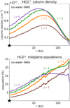 |
Fig. 7 HCO+ column density (top) and midplane populations (bottom) for the J = 1 (brown), J = 2 (orange), J = 3 (green), and J = 4 (purple) levels as a function of radius for chemical network NW in the typical Herbig disk model. |
3.3 Line profiles
The discussion above has shown that locating the water snowline using the HCO+ radial emission profile is difficult. The velocity resolved line profile may provide an alternative method as the removal of HCO+ in the inner disk is expected to remove flux at the highest Keplerian velocities. Therefore, the line profile predicted by chemical network W is expected to be narrower than the line profile predicted by network NW.
The line profiles predicted by the two chemical networks for the J = 2−1 transition of HCO+ and H13 CO+ are shown in left column of Fig. 8. To show the difference between the models we subtracted the spectrum associated with network W from the spectrum associated with network NW. The result is shown in the right column of Fig. 8. This column shows that even though the line profiles look almost identical in the left column, there is an additional bump in the difference between them in the line wings (indicated with the black arrows). However, this difference is only 1.75 mJy for HCO+ and 28 μJy for H13 CO+, that is, 0.6 and 0.3% of emission, which cannot be detected with a reasonable signal-to-noise ratio with current submillimetre observations. Moreover, detailed comparison with the line profile associated with a molecule that does not show a decrease in the column density in the inner disk would be needed as only the flux associated with network W would be observed, and not the flux associated with network NW. Hence, it is very difficult to use the line profiles to locate the water snowline in disks around Herbig Ae stars.
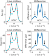 |
Fig. 8 Predicted HCO+ and H13CO+ line profiles in a typical Herbig Ae disk. Left panels: line profile for the J = 2− 1 transition of HCO+ (top) and H13CO+ (bottom) forchemical network NW (red) and W (light blue). Right panels: difference between the line profiles in the left column. The black arrows indicate where the effect of the water snowline is expected. We note the differences in the vertical axes. |
4 Comparison with observations
The best targets to observe the water snowline using HCO+ are warm disks because these disks have a water snowline at a large enough radius for ALMA to resolve. In addition, disks without deep gaps in the gas and dust surface density around the expected location of the snowline are preferred, as these gaps complicate the interpretation of the HCO+ emission.
One of the most promising targets to locate the water snowline in a disk is the young outbursting star V883 Ori, with a current luminosity of ~218 L⊙ (Furlan et al. 2016). During the outburst, the luminosity is greatly increased, which heats the disk, shifting the water snowline outwards compared to regular T Tauri and even Herbig Ae disks. This not only allows for observations with a larger beam, it also mitigates the effects of the dust as the optical depth of the continuum emission decreases with radius. Previous observations of V883 Ori have inferred the location of the water snowline at 42 AU based on a change in the dust emission (Cieza et al. 2016). An extended hot inner disk region is consistent with the detection of many complex organic molecules (Lee et al. 2019). However, an abrupt change in the continuum optical depth or the spectral index are not necessarily due to a snowline, as shown for the cases of CO2, CO, and N2 (Huang et al. 2018; Long et al. 2018; van Terwisga et al. 2018). Methanol observations suggest that the water snowline may be located at a much larger radius of ~100 AU, if the methanol observations are optically thin and most of its emission originates from inside the water snowline (van ’t Hoff et al. 2018b). Observations of HCO+ have the potential to resolve this discrepancy.
4.1 H13 CO+ observations
A promising dataset to locate the water snowline in V883 Ori is the band 7 observation by Lee et al. (2019) (project code: 2017.1.01066.T, PI: Jeong-Eun Lee), which contains the H13 CO+ J = 4−3 line. To date, these observations are the only H13 CO+ observations in a protoplanetary disk, to our knowledge, at sufficient spatial and spectral resolution and with enough sensitivity to potentially resolve the water snowline. The synthesised beam of these observations is 0′′.2 (40 AU radius, 80 AU diameter at a distance of ~400 pc; Kounkel et al. 2017), and the spectral resolution is 0.25 km s−1. The continuum is created using all line-free channels, which are carefully selected to exclude any line emission. The line data are continuum subtracted using these continuum solutions. Using the CASA 5.1.1 tclean task with a Briggs weighting of 0.5, line images are made with a mask of about 2″ in diameter centred on the peak of the continuum.
Following the approach of Lee et al. (2019), the line observations are velocity-stacked using a stellar mass, M⋆ = 1.3 M⊙, an inclination of 38°, and a position angle of 32° (Cieza et al. 2016). This technique reduces line blending because it makes use of the Keplerian velocity of the disk to calculate the Doppler shift of the emission in each pixel (Yen et al. 2016, 2018). This Doppler shift is then used to shift the spectrum of each pixel to the velocity of the star, before adding the spectra of all pixels. The noise level of ~15 mJy per spectral bin is determined using an empty region in the stacked image.
The resulting spectrum of the inner 0′′.6 is shown as the black line in the top panel of Fig. 9. The rest frequency of the H13 CO+ J = 4−3 transition lies between the rest frequencies of the 187,12–177,11, E transition of acetaldehyde (CH3CHO) (v = 0) at 346.9955 GHz and the two superimposed 187,11 – 177,10, E and 187,12 – 177,11, E transitions of CH3CHO (vT = 2) at 346.99991 and 346.99994 GHz, respectively (Jet Propulsion Laboratory (JPL) molecular database; Pickett et al. 1998). In between these acetaldehyde transitions, a clear shoulder of emission is visible due to the J = 4−3 transition of H13 CO+. To quantifythis excess emission, two Gaussian profiles are fitted with curve_fit2 to model the acetaldehyde emission. To reduce the number of free parameters in the fit, the line frequencies are fixed to their respective rest frequencies listed above and the widths of the lines are fixed to 2 km s−1 following Lee et al. (2019). In addition, emission within 1 km s−1 from the rest frequency of the J = 4−3 transition of H13 CO+ is excluded from the fit. The result is shown as the red line in the top panel of Fig. 9. Subtracting this fit to the acetaldehyde emission from the observed spectrum clearly reveals emission of the J = 4−3 transition of H13 CO+. Therefore, we conclude that H13 CO+ is detected at >5σ but is blended with lines that are expected to peak on-source, preventing a clean image.
The line blending of H13 CO+ J = 4−3 with acetaldehyde prevents us from using the only available dataset covering a transition of H13 CO+ at sufficient spatial and spectral resolution, and sensitivity to resolve the water snowline. The J = 3−2 transition of H13 CO+ is likely blended with CH3OCHO as both of them are bright in the Class 0 source B1-c (van Gelder et al. 2020). However, the H13 CO+ J = 2−1 transition in the same Class 0 B1-c source is free from line blending (van ’t Hoff et al., in prep.) and would therefore be the best line to target in sources with bright emission from complex organics.
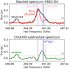 |
Fig. 9 Observed and modelled spectrum of V883 Ori. Top panel: observed and stacked spectrum of V883 Ori (black) and a fit of the CH3CHO emission (red). Bottom panel: spectrum where the CH3CHO emission is subtracted. The H13CO+ J = 4− 3 emission line(vertical dark blue line) is blended with the CH3CHO lines (vertical pink lines). The 3σ noise level is indicated with the horizontal grey line. |
4.2 HCO+ observations
Another promising dataset for HCO+ is a recent band 6 dataset (project code 2018.1.01131.S, PI: D. Ruíz-Rodríguez; Ruíz-Rodríguez et al., in prep.). The J = 3−2 transition of HCO+ is detected with a high signal-to-noise ratio. The spatial resolution of ~ 0′′.5 is insufficient to resolve the water snowline if it is located within a radius of ~ 90 AU (180 AU diameter).
An image of the HCO+ emission will be presented in Ruíz-Rodríguez et al. (in prep.). Here, a normalised, deprojected azimuthal average of the observed emission from the product data of the J = 3−2 transition ofHCO+ is presentedin the top panel of Fig. 10. This azimuthal average shows that the HCO+ emission is ring shaped. Comparing the band 6 HCO+ emission with the band 7 emission from complex organic molecules presented in van ’t Hoff et al. (2018b) and Lee et al. (2019), reveals that the emission from complex organic molecules such as methanol, 13-methanol, acetaldehyde, and H2 C18O peak inside the HCO+ ring, and insome cases is even centrally peaked. This is a strong indication that the lack of HCO+ emission in the centre is not only due to the optical depth of the continuum and that HCO+ is indeed tracing the water snowline in V883 Ori. Such an anti-correlation between HCO+ and methanol has also been seen in protostellar envelopes (Jørgensen et al. 2013).
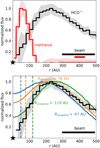 |
Fig. 10 Observed and modelled emission from HCO+ J = 3− 2 and observed methanol in V883 Ori. Top: normalised azimuthal average of the observed HCO+ J = 3− 2 flux in V883 Ori (black; Ruíz-Rodríguez et al., in prep. and this work) and methanol 183 –174 flux (red; van ’t Hoff et al. 2018b). Bottom: normalised azimuthal average of the observed HCO+ flux (black; as in top panel) and modelled HCO+ flux for a snowline at 47 AU (blue), 76 AU (orange), and 119 AU (green). The snowline locations of the models are indicated with dashed lines in corresponding colours. The position of the star is indicated with a black star and the beam is indicated by the black bar in the bottom right corner. |
4.3 Model HCO+ images: locating the snowline
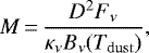
To quantifythe location of the water snowline, we model the HCO+ and H13 CO+ emission in a representative model for V883 Ori. This model reproduces the previously observed flux of the J = 2−1 transition of C18 O (van ’t Hoff et al. 2018b), the HCO+ and H13 CO+ total flux discussed in the previous Sections, and mm continuum fluxes within a factor of ~2. The DALI model parameters are presented in Table D.1. The main changes compared to the model for the typical Herbig Ae disk include the mass and radius of the disk, and the mass and luminosity of the star. The characteristic disk radius is set to 75 AU to match the radial extent of emission from the J = 2−1 transition of C18O presented by van ’t Hoff et al. (2018b). The disk mass is estimated using the 9.1 mm continuum observations of the VANDAM survey (Tobin et al. 2020) and the relation between the continuum flux and the disk mass (Hildebrand 1983):
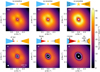 |
Fig. 11 Integrated intensity maps for the J = 3−2 transition of HCO+ predicted by network NW (top row) and network W (bottom row). The snowline is indicated with a white ellipse and is located at 47 AU (left column), 76 AU (middle column), and 119 AU (right column). The cartoons above the individual panels provide a sketch of the model, where blue indicates water ice, red indicates gas-phase water, orange indicates a high abundance of HCO+, and grey indicates a low abundance of HCO+. The position of the star is marked with a yellow star in each cartoon and with white star in each panel. We note that the size of the star increases with increasing luminosity of the star. The 0′′.1 beam and a scale bar are indicated in the bottom left panel. |
 (10)
(10)
with D the distance to V883 Ori, Fν the observed continuum flux, κν the opacity, and Bν (Tdust) the Planck function for a dust temperature Tdust. As V883 Ori is an outbursting source, a dust temperature of 50 K is assumed. Following Tychoniec et al. (2020), a dust opacity of 0.28 cm2 g−1 at a wavelength of 9.1 mm is used (Woitke et al. 2016). This results in an estimated disk mass of 0.25 M⊙.
The water snowline has been estimated at 42 AU by Cieza et al. (2016), but it may be as far out as 100 AU based on CH3OH observations (van ’t Hoff et al. 2018b). The outburst likely began before 1888 (Pickering 1890) and has been decreasing since. Approximately 25 yr ago the luminosity was measured to be ~200 L⊙ higher than the current value (Strom & Strom 1993; Sandell & Weintraub 2001; Furlan et al. 2016). With a freeze-out time scale of 100–1000 yr, the water snowline may thus not be at the location expected from the current luminosity (Jørgensen et al. 2013; Visser et al. 2015; Hsieh et al. 2019). We therefore use three different luminosities of 2 × 10³, 6 × 10³, and 1.4 × 10⁴ L⊙ in our models, which put the snowline at 47, 76, and 119 AU, respectively.
The resulting integrated intensity maps of the J = 3−2 transition of HCO+ for these models are shown in Fig. 11. The corresponding figures for the weaker HCO+ and H13 CO+ J = 2−1 transitions are presented in Figs. D.1 and D.2. These lines are not expected to be contaminated by emission from complex organic molecules. The results in this section are convolved with a small 0′′.1 beam to make predictions for future high resolution observations.
The top row of Fig. 11 shows the expected emission for network NW for the three different luminosities. The total HCO+ emission does not depend strongly on the luminosity because the population of the J = 3 level decreases with luminosity but the increase in the temperature of the emitting region cancels this effect as the HCO+ emission is marginally optically thick. Similar to the models for a disk around a typical Herbig Ae star, the moment 0 maps of network NW show ring shaped emission despite the fact that there is no snowline present in these models. The lack of emission in the centre is dominated by absorption by dust. On top of that, the column density of the J = 3 level of HCO+ decreases in the inner parts of the disk. These two points are difficult to disentangle because the continuum optical depth is frequency and hence J-level dependent. However, most importantly, the location of the HCO+ ring does not change as a function of luminosity in network NW.
This is different in the bottom row of Fig. 11, where emission associated with network W is shown. The water snowline is indicated with a white ellipse and shifts outwards as the luminosity of the star increases. This is also reflected in the HCO+ emission as the ring of HCO+ shifts outwards together with the water snowline. Therefore, the location of the HCO+ ring can be used to locate the water snowline provided that another molecule is observed to show that the decrease in the HCO+ flux in the centre is not solely due to molecular excitation effects and absorption by dust. The excitation effect needs to be inferred from disk modelling. The effect of the optical depth of the continuum emission can be estimated by observing another molecule, that emits from the same disk region as HCO+ and whose column density does not drop in the inner disk. The most obvious molecule for this purpose is C18 O. However, the HCO+ J = 3−2 emission comes from a layer closer to the midplane than the C18O J = 2−1 and J = 3−2 emission. Therefore, the effect of the dust on the HCO+ emission cannot be fully traced by the J = 2−1 or J = 3−2 transition of C18 O. Rarer isotopologues such as C17O or 13 C18O are more suited for this purpose, as well as other molecules such as complex organics as discussed in Sect. 4.2.
The model predictions for the observed flux of the J = 3−2 transition of HCO+ in V883 Ori are compared with the observed flux in the bottom panel of Fig. 10. The model results are convolved to the same spatial resolution as the observations before calculating the deprojected azimuthal average. Even though the beam is too large to resolve the snowline if it is located inside ~ 90 AU, this figure clearly shows that the observed HCO+ flux drops off steeper in the inner parts than that predicted by the model with a snowline at 47 AU. In addition, the HCO+ ring shifts outwards with increasing snowline location. The observed peak location and gap depth in the centre best match with a snowline between 76 and 119 AU.
A central cavity (approx. 1 beam in diameter at 0′′.35 × 0′′.27 resolution corresponding to ~60 AU resolution in radius) was also observed for CO J = 2−1 and was attributed to the continuum optical depth by Ruíz-Rodríguez et al. (2017). However, it is unlikely that the cavity observed in HCO+ is solely due to the continuum as the emission from complex organic molecules peaks inside the HCO+ ring (0′′.23 × 0′′.17; Lee et al. 2019). Similarly, the high resolution methanol emission (0′′.13 × 0′′.14; van ’t Hoff et al. 2018b) and the continuum emission (0′′.03; Cieza et al. 2016) peak well inside the HCO+ cavity (Fig. 10). Furthermore, the continuum becomes optically thin well within 100 AU in all three of our models (Figs. 10 and 11), so the difference between the models is due to different snowline locations. Therefore, our analysis is consistent with a water snowline at ~75–120 AU in V883 Ori, and thus suggests that the sudden change in continuum opacity at 42 AU is uncorrelated with the water snowline.
One effect that needs to be taken into account in outbursting sources like V883 Ori is viscous heating. This effect heats the disk midplane, hence the water snowline could be at a larger radius than expected based on radiative heating alone. The J = 3−2 transition of HCO+ is marginally optically thick in our models. Targeting a low J transition of HCO+ or targeting the optically thin H13 CO+, will allow us to directly trace the midplane. Another effect that could occur due to viscous heating is self-absorption of HCO+ as the surface layers of the disk could have a lower temperature than the viscously heated midplane. This, again, could be resolved by observing multiple transitions of HCO+ as higher J lines are more optically thick and hence trace a layer higher in the disk.
Taken together, our analysis of the observations suggests that HCO+ is tracing the water snowline in the V883 Ori disk, and that the snowline is located outside the radius where the change in the continuum opacity is observed. Therefore, V883 Ori is the first example that shows that a change in the dust continuum opacity is not necessarily related to the water snowline, similar to what has been shown for the cases of CO, CO2, and N2 snowlines (Huang et al. 2018; Long et al. 2018; van Terwisga et al. 2018).
5 Conclusions
Chemical imaging with HCO+ is in principle a promising method to image the water snowline as it has been used successfully in a protostellar envelope (van ’t Hoff et al. 2018a). This work examines the application of this to older protoplanetary disks. The HCO+ abundance was modelled using two chemical networks, one with water (W) and one without water (NW). Predictions for the radial emission profiles of HCO+ and H13 CO+ were made to examine the validity of HCO+ as a tracer of the water snowline. Moreover, archival observations of V883 Ori were examined to constrain the location of the water snowline in V883 Ori and make predictions for future high resolution observations.
Based on our models the following conclusions can be drawn:
-
The HCO+ abundance jumps two orders of magnitude around the water snowline.
-
In addition to the water snowline, the optical depth of the continuum emission and molecular excitation effects for the low J-levels contribute significantly to the decrease in the H13CO+ and HCO+ flux in the inner parts of the disk and result in ring shaped emission. Therefore, the effect of the continuum optical depth needs to be checked observationally, and the effects of the molecular excitation and HCO+ abundance need to be modelled in detail. Outbursting sources are the best targets, as the snowline is shifted to larger radii, where the dust optical depth is lower.
-
HCO+ and H13CO+ are equally good as a tracers of the water snowline but the main isotopologue HCO+ is more readily observable because of its higher abundance.
-
For both HCO+ and H13CO+, the J = 2−1 transition is preferred because it provides the best balance between line strength and the negative effects of the continuum optical depth. Moreover, it is not expected to be blended with emission from complex organic molecules, unlike the J = 3−2 and J = 4−3 transitions of H13CO+.
-
Our analysis of the observations of the HCO+ J = 3−2 transition and complex organic molecules suggest that HCO+ is tracing the water snowline in V883 Ori. Based on our models, the snowline is located around 100 AU and is not correlated with the opacity change in the continuum emission observed at 42 AU.
Our results thusshow that HCO+ and H13 CO+ can be used to trace the water snowline in warm protoplanetary disks, such as those found around luminous stars. Determining the snowline location in these sources is important to understand the process of planet formation and composition.
Acknowledgements
We thank the referee and the editor for the constructive comments, and Catherine Walsh and Jeong-Eun Lee for useful discussions. Astrochemistry in Leiden is supported by the Netherlands Research School for Astronomy (NOVA). M.L.R.H acknowledges support from a Huygens fellowship from Leiden University, and from the Michigan Society of Fellows. L.T. is supportedby NWO grant 614.001.352. This paper makes use of the following ALMA data: ADS/JAO.ALMA#2017.1.01066.T. and ADS/JAO.ALMA#2018.1.01131.S. ALMA is a partnership of ESO (representing its member states), NSF (USA) and NINS (Japan), together with NRC (Canada), MOST and ASIAA (Taiwan), and KASI (Republic of Korea), in cooperation with the Republic of Chile. The Joint ALMA Observatory is operated by ESO, AUI/NRAO and NAOJ.
Appendix A Freeze-out and desorption coefficients
The reaction coefficients of the freeze-out and desorption of water depend on the local conditions in the disk. The rate coefficient of the freeze-out of water, kf can be expressed as:

where 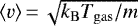 is the thermal velocity of gas-phase water molecules with mass m in a gas at temperature Tgas, and kB is the Boltzmann constant. The DALI models use a distribution of grain sizes, but for the chemistry, only the surface area of the grains matters. Therefore, a grain size of agrain = 0.1 μm and a number density, n(grain) = 10−12 × n(H2) with respect to molecular hydrogen is used. Finally, a sticking coefficient, S, of 1 is assumed.
The reverse process, the desorption of water ice, is described by the desorption rate coefficient:

with 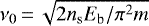 the characteristic vibrational frequency of water ice on a grain. Here ns = 1.5 × 1015 cm−2 is the number density of surface sites where water can bind (Hasegawa et al. 1992). The binding energy, Eb, assumed in this work is 5775 K, corresponding to an amorphous water ice substrate (Fraser et al. 2001).
Appendix B Chemical network
B.1 Analytical approximation for network NW
Chemical network NW can be used to derive an analytical expression for the HCO+ abundance because of its simplicity. The time evolution of the HCO+ number density is given by the sum of the formation and destruction rates:
 (B.1)
(B.1)
with k4 and  the reaction rates as listed in Table 2. This can be rewritten to
 (B.2)
(B.2)
under the assumption of steady state. Furthermore, it is assumed that metallic ions can be neglected as electron donors, and that HCO+ is the main electron donor. HCO+ has been found to be the dominant molecular ion protoplanetary disks (Teague et al. 2015), and the main charge carrier in starless cores (e.g. Caselli et al. 1998; Williams et al. 1998).
Following the approach of Lepp et al. (1987), the number density of H , which is mainly governed by the ionisation, can be found in a similar way. The three reactions that regulate the ionisation in the disk: ionisation by cosmic rays (reaction ζcr), the ion-molecule reaction to form H
 (reaction k2), and dissociative recombination of H
 (reaction k3), see also Table 2. The first two reactions can be approximated as:
Initial conditions for chemical network NW (no water) and W (water).
 (B.3)
(B.3)
as the formation of H is limited by the cosmic ray ionisation rate. Assuming CO is the main destroyer of H
 and thus neglecting the dissociative recombination of H
 , the time evolution and steady state abundance of H
 can be expressed as:

Combining Eqs. (B.2) and (B.5) gives the analytical approximation of the HCO+ abundance in the disk:
 (B.6)
(B.6)
The comparison of chemical network NW and W in Sect. 3.1 and Fig. 3 shows that the HCO+ abundance in network NW is very similar to the HCO+ abundance outside the water snow surface in network W. Therefore, the derived expression for the HCO+ abundance can also be used in this disk region in chemical network W.
B.2 Initial conditions
The effects of the initial conditions on the abundance predicted by chemical network W were discussed in Sect. 3.1.2 and expected to be of little importance for HCO+’s ability to trace the water snowline. Here, the effects on the corresponding radial emission profiles of the J = 2−1 transition of HCO+ and H13 CO+ are discussed and shown in Fig. B.1.
Previously, it was derived that the column density of HCO+ scales with the square root of the cosmic ray ionisation rate (see Eq. (9)). Similarly, the H13 CO+ emission scales with the square root of the cosmic ray ionisation rate because it is optically thin, see Fig. B.1. On the other hand, the HCO+ emission does not scale with the cosmic ray ionisation rate as it is optically thick. As the column density of HCO+ decreases, the HCO+ emission becomes less optically thick and approaches the scaling for the column density.
In Sect. 3.1.2, it was found that the HCO+ abundance or column density does not depend strongly on the initial abundance of CO or H2 O. This is is also seen in the radial emission profiles both for HCO+ and H13 CO+ because the drop in the HCO+ emission in the centre is dominated by the effect of the optical depth of the continuum emission and molecular excitation. A small dependence of the HCO+ emission on the initial abundance of gas-phase water is seen, but the abundance of gas-phase water seems to be low in the outer regions of protoplanetary disks (Bergin et al. 2010; Du et al. 2017; Notsu et al. 2019; Harsono et al. 2020). Moreover, the abundance of gas-phase water in the inner disk can be as high as 10−2 (Bosman et al. 2018).
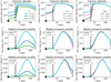 |
Fig. B.1 HCO+ column densities for different initial conditions in chemical network W (top row) and the corresponding radial emission profiles for the J = 2−1 transition of HCO+ (middle row) and H13CO+ (bottom row). Left-hand column: results for a cosmic ray ionisation rate of 10−17, 10−18, and 10−19s−1. Middle column: corresponding models for an initial CO abundance of 10−4, 10−5, and 10−6. Right-hand column: corresponding models for an initial abundance of gas-phase water of 3 × 10⁻⁵, 3 × 10⁻⁶, and 3.8 × 10⁻⁷. The fiducial model is indicated with the light blue line in each panel and uses an initial abundance of 3.8 × 10⁻⁷ for gas-phase water, 10−4 for gas-phase CO, and 10−17s−1 for the cosmic ray ionisation rate. The water snowline is indicated with a dashed black line and the position of the star is indicated by the symbol of a black star. The radial emission profiles are convolved with a 0′′.05 beam. |
Appendix C HCO+ and H13 CO+ J = 1–0, J = 3–2, and J = 4–3 transitions
Radial emission profiles for the J = 1−0, J = 3−2, and J = 4−3 transitions of HCO+ and H13 CO+ are presented in Fig. C.1.
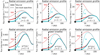 |
Fig. C.1 Same as the middle and bottom panel of Fig. 5, but then for the J = 1− 0 (left column), J = 3−2 (middle column), and J = 4−3 (right column) transition of HCO+ (top) and H13CO+ (bottom). |
Appendix D V883 Ori
An overview of the model parameters used for the representative DALI model for V883 Ori is given in Table D.1. Predictions for the corresponding emission of the J = 2−1 transition of HCO+ and H13 CO+ are shown in Figs. D.1 and D.2.
DALI model parameters for the representative model for V883 Ori.
 |
Fig. D.1 Same as Fig. 11 but then for the J = 2−1 transition of HCO+. The 0′′.1 beam and a scale bar are indicated in the bottom left panel. |
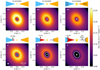 |
Fig. D.2 Same as Fig. 11 but then for the J = 2−1 transition of H13CO+. The 0′′.1 beam and a scale bar are indicated in the bottom left panel. |
References
- Adams, N. G., Smith, D., & Grief, D. 1978, Int. J. Mass Spectrom. Ion Process., 26, 405 [NASA ADS] [CrossRef] [Google Scholar]
- Agúndez, M., Roueff, E., Le Petit, F., & Le Bourlot, J. 2018, A&A, 616, A19 [NASA ADS] [CrossRef] [EDP Sciences] [Google Scholar]
- Aikawa, Y., Furuya, K., Nomura, H., & Qi, C. 2015, ApJ, 807, 120 [NASA ADS] [CrossRef] [Google Scholar]
- Andrews, S. M. 2020, ARA&A, 58, 483 [CrossRef] [Google Scholar]
- Andrews, S. M., Wilner, D. J., Hughes, A. M., Qi, C., & Dullemond, C. P. 2010, ApJ, 723, 1241 [NASA ADS] [CrossRef] [Google Scholar]
- Andrews, S. M., Wilner, D. J., Espaillat, C., et al. 2011, ApJ, 732, 42 [Google Scholar]
- Anicich, V. G., Futrell, J. H., Huntress, W. T., J., & Kim, J. K. 1975, Int. J. Mass Spectrom. Ion Process., 18, 63 [NASA ADS] [CrossRef] [Google Scholar]
- Banzatti, A., Pinilla, P., Ricci, L., et al. 2015, ApJ, 815, L15 [NASA ADS] [CrossRef] [Google Scholar]
- Banzatti, A., Pontoppidan, K. M., Salyk, C., et al. 2017, ApJ, 834, 152 [NASA ADS] [CrossRef] [Google Scholar]
- Bergin, E. A., Melnick, G. J., & Neufeld, D. A. 1998, ApJ, 499, 777 [NASA ADS] [CrossRef] [MathSciNet] [Google Scholar]
- Bergin, E. A., Hogerheijde, M. R., Brinch, C., et al. 2010, A&A, 521, L33 [NASA ADS] [CrossRef] [EDP Sciences] [Google Scholar]
- Blevins, S. M., Pontoppidan, K. M., Banzatti, A., et al. 2016, ApJ, 818, 22 [NASA ADS] [CrossRef] [Google Scholar]
- Booth, A. S., & Ilee, J. D. 2020, MNRAS, 493, L108 [CrossRef] [Google Scholar]
- Booth, A. S., Walsh, C., Ilee, J. D., et al. 2019, ApJ, 882, L31 [NASA ADS] [CrossRef] [Google Scholar]
- Bosman, A. D., Tielens, A. G. G. M., & van Dishoeck, E. F. 2018, A&A, 611, A80 [NASA ADS] [CrossRef] [EDP Sciences] [Google Scholar]
- Botschwina, P., Horn, M., Flügge, J., & Seeger, S. 1993, J. Chem. Soc. Faraday Trans., 89, 2219 [CrossRef] [Google Scholar]
- Bruderer, S. 2013, A&A, 559, A46 [NASA ADS] [CrossRef] [EDP Sciences] [Google Scholar]
- Bruderer, S., Doty, S. D., & Benz, A. O. 2009, ApJS, 183, 179 [NASA ADS] [CrossRef] [Google Scholar]
- Bruderer, S., van Dishoeck, E. F., Doty, S. D., & Herczeg, G. J. 2012, A&A, 541, A91 [NASA ADS] [CrossRef] [EDP Sciences] [Google Scholar]
- Bryden, G., Chen, X., Lin, D. N. C., Nelson, R. P., & Papaloizou, J. C. B. 1999, ApJ, 514, 344 [NASA ADS] [CrossRef] [Google Scholar]
- Carney, M. T., Fedele, D., Hogerheijde, M. R., et al. 2018, A&A, 614, A106 [NASA ADS] [CrossRef] [EDP Sciences] [Google Scholar]
- Carr, J. S., & Najita, J. R. 2008, Science, 319, 1504 [NASA ADS] [CrossRef] [PubMed] [Google Scholar]
- Caselli, P., Walmsley, C. M., Terzieva, R., & Herbst, E. 1998, ApJ, 499, 234 [NASA ADS] [CrossRef] [Google Scholar]
- Cazzoletti, P., van Dishoeck, E. F., Visser, R., Facchini, S., & Bruderer, S. 2018, A&A, 609, A93 [NASA ADS] [CrossRef] [EDP Sciences] [Google Scholar]
- Cieza, L. A., Casassus, S., Tobin, J., et al. 2016, Nature, 535, 258 [NASA ADS] [CrossRef] [Google Scholar]
- D’Alessio, P., Calvet, N., Hartmann, L., Franco-Hernández, R., & Servín, H. 2006, ApJ, 638, 314 [NASA ADS] [CrossRef] [Google Scholar]
- Dong, R., Liu, S.-y., Eisner, J., et al. 2018, ApJ, 860, 124 [NASA ADS] [CrossRef] [Google Scholar]
- Drążkowska, J., & Alibert, Y. 2017, A&A, 608, A92 [NASA ADS] [CrossRef] [EDP Sciences] [Google Scholar]
- Du, F., Bergin, E. A., Hogerheijde, M., et al. 2017, ApJ, 842, 98 [NASA ADS] [CrossRef] [Google Scholar]
- Eistrup, C., Walsh, C., & van Dishoeck, E. F. 2016, A&A, 595, A83 [NASA ADS] [CrossRef] [EDP Sciences] [Google Scholar]
- Eistrup, C., Walsh, C., & van Dishoeck, E. F. 2018, A&A, 613, A14 [NASA ADS] [CrossRef] [EDP Sciences] [Google Scholar]
- Fedele, D., Carney, M., Hogerheijde, M. R., et al. 2017, A&A, 600, A72 [NASA ADS] [CrossRef] [EDP Sciences] [Google Scholar]
- Flower, D. R. 1999, MNRAS, 305, 651 [NASA ADS] [CrossRef] [Google Scholar]
- Fraser, H. J., Collings, M. P., McCoustra, M. R. S., & Williams, D. A. 2001, MNRAS, 327, 1165 [NASA ADS] [CrossRef] [Google Scholar]
- Furlan, E., Fischer, W. J., Ali, B., et al. 2016, ApJS, 224, 5 [NASA ADS] [CrossRef] [Google Scholar]
- Harsono, D., Bruderer, S., & van Dishoeck, E. F. 2015, A&A, 582, A41 [NASA ADS] [CrossRef] [EDP Sciences] [Google Scholar]
- Harsono, D., Persson, M. V., Ramos, A., et al. 2020, A&A, 636, A26 [CrossRef] [EDP Sciences] [Google Scholar]
- Hartmann, L., Calvet, N., Gullbring, E., & D’Alessio, P. 1998, ApJ, 495, 385 [NASA ADS] [CrossRef] [Google Scholar]
- Hasegawa, T. I., Herbst, E., & Leung, C. M. 1992, ApJS, 82, 167 [NASA ADS] [CrossRef] [Google Scholar]
- Hildebrand, R. H. 1983, QJRAS, 24, 267 [NASA ADS] [Google Scholar]
- Hogerheijde, M. R., Bergin, E. A., Brinch, C., et al. 2011, Science, 334, 338 [NASA ADS] [CrossRef] [PubMed] [Google Scholar]
- Hsieh, T.-H., Murillo, N. M., Belloche, A., et al. 2019, ApJ, 884, 149 [NASA ADS] [CrossRef] [Google Scholar]
- Huang, J., Andrews, S. M., Dullemond, C. P., et al. 2018, ApJ, 869, L42 [NASA ADS] [CrossRef] [Google Scholar]
- Isella, A., Guidi, G., Testi, L., et al. 2016, Phys. Rev. Lett., 117, 251101 [NASA ADS] [CrossRef] [Google Scholar]
- Jørgensen, J. K., Visser, R., Sakai, N., et al. 2013, ApJ, 779, L22 [NASA ADS] [CrossRef] [Google Scholar]
- Kama, M., Bruderer, S., van Dishoeck, E. F., et al. 2016, A&A, 592, A83 [NASA ADS] [CrossRef] [EDP Sciences] [Google Scholar]
- Kama, M., Trapman, L., Fedele, D., et al. 2020, A&A, 634, A88 [CrossRef] [EDP Sciences] [Google Scholar]
- Kim, J. K., Theard, L. P., & Huntress, W. T., J. 1974, Int. J. Mass Spectrom. Ion Process., 15, 223 [NASA ADS] [CrossRef] [Google Scholar]
- Kimura, H., Wada, K., Kobayashi, H., et al. 2020, MNRAS, 498, 1801 [CrossRef] [Google Scholar]
- Klippenstein, S. J., Georgievskii, Y., & McCall, B. J. 2010, J. Phys. Chem. A, 114, 278 [CrossRef] [Google Scholar]
- Kounkel, M., Hartmann, L., Loinard, L., et al. 2017, ApJ, 834, 142 [NASA ADS] [CrossRef] [Google Scholar]
- Lee, J.-E., Lee, S., Baek, G., et al. 2019, Nat. Astron., 3, 314 [NASA ADS] [CrossRef] [Google Scholar]
- Lepp, S., Dalgarno, A., & Sternberg, A. 1987, ApJ, 321, 383 [NASA ADS] [CrossRef] [Google Scholar]
- Long, F., Pinilla, P., Herczeg, G. J., et al. 2018, ApJ, 869, 17 [NASA ADS] [CrossRef] [Google Scholar]
- Lynden-Bell, D., & Pringle, J. E. 1974, MNRAS, 168, 603 [NASA ADS] [CrossRef] [Google Scholar]
- Mandell, A. M., Bast, J., van Dishoeck, E. F., et al. 2012, ApJ, 747, 92 [NASA ADS] [CrossRef] [Google Scholar]
- Mathews, G. S., Klaassen, P. D., Juhász, A., et al. 2013, A&A, 557, A132 [NASA ADS] [CrossRef] [EDP Sciences] [Google Scholar]
- Mathis, J. S., Rumpl, W., & Nordsieck, K. H. 1977, ApJ, 217, 425 [NASA ADS] [CrossRef] [Google Scholar]
- McCall, B. J., Huneycutt, A. J., Saykally, R. J., et al. 2004, Phys. Rev. A, 70, 052716 [NASA ADS] [CrossRef] [Google Scholar]
- McElroy, D., Walsh, C., Markwick, A. J., et al. 2013, A&A, 550, A36 [NASA ADS] [CrossRef] [EDP Sciences] [Google Scholar]
- Milam, S. N., Savage, C., Brewster, M. A., Ziurys, L. M., & Wyckoff, S. 2005, ApJ, 634, 1126 [NASA ADS] [CrossRef] [Google Scholar]
- Mitchell, J. B. A. 1990, Phys. Rep., 186, 215 [NASA ADS] [CrossRef] [Google Scholar]
- Notsu, S., Akiyama, E., Booth, A., et al. 2019, ApJ, 875, 96 [NASA ADS] [CrossRef] [Google Scholar]
- Novotný, O., Buhr, H., Stützel, J., et al. 2010, J. Phys. Chem. A, 114, 4870 [CrossRef] [PubMed] [Google Scholar]
- Öberg, K. I., Murray-Clay, R., & Bergin, E. A. 2011, ApJ, 743, L16 [NASA ADS] [CrossRef] [Google Scholar]
- Okuzumi, S., Momose, M., Sirono, S.-i., Kobayashi, H., & Tanaka, H. 2016, ApJ, 821, 82 [NASA ADS] [CrossRef] [Google Scholar]
- Phillips, T. G., van Dishoeck, E. F., & Keene, J. 1992, ApJ, 399, 533 [NASA ADS] [CrossRef] [Google Scholar]
- Pickering, E. C. 1890, Ann. Harvard College Observ., 18, 1 [Google Scholar]
- Pickett, H. M., Poynter, R. L., Cohen, E. A., et al. 1998, J. Quant. Spectr. Rad. Transf., 60, 883 [Google Scholar]
- Pinilla, P., Pohl, A., Stammler, S. M., & Birnstiel, T. 2017, ApJ, 845, 68 [NASA ADS] [CrossRef] [Google Scholar]
- Qi, C., Öberg, K. I., Wilner, D. J., et al. 2013, Science, 341, 630 [NASA ADS] [CrossRef] [PubMed] [Google Scholar]
- Qi, C., Öberg, K. I., Andrews, S. M., et al. 2015, ApJ, 813, 128 [NASA ADS] [CrossRef] [Google Scholar]
- Qi, C., Öberg, K. I., Espaillat, C. C., et al. 2019, ApJ, 882, 160 [NASA ADS] [CrossRef] [Google Scholar]
- Ruíz-Rodríguez, D., Cieza, L. A., Williams, J. P., et al. 2017, MNRAS, 468, 3266 [NASA ADS] [CrossRef] [Google Scholar]
- Salinas, V. N., Hogerheijde, M. R., Bergin, E. A., et al. 2016, A&A, 591, A122 [NASA ADS] [CrossRef] [EDP Sciences] [Google Scholar]
- Salyk, C., Pontoppidan, K. M., Blake, G. A., et al. 2008, ApJ, 676, L49 [NASA ADS] [CrossRef] [Google Scholar]
- Salyk, C., Lacy, J., Richter, M., et al. 2019, ApJ, 874, 24 [CrossRef] [Google Scholar]
- Sandell, G., & Weintraub, D. A. 2001, ApJS, 134, 115 [NASA ADS] [CrossRef] [Google Scholar]
- Schöier, F. L., van der Tak, F. F. S., van Dishoeck, E. F., & Black, J. H. 2005, A&A, 432, 369 [NASA ADS] [CrossRef] [EDP Sciences] [Google Scholar]
- Schoonenberg, D., & Ormel, C. W. 2017, A&A, 602, A21 [NASA ADS] [CrossRef] [EDP Sciences] [Google Scholar]
- Stevenson, D. J., & Lunine, J. I. 1988, Icarus, 75, 146 [NASA ADS] [CrossRef] [Google Scholar]
- Strom, K. M., & Strom, S. E. 1993, ApJ, 412, L63 [NASA ADS] [CrossRef] [Google Scholar]
- Teague, R., Semenov, D., Guilloteau, S., et al. 2015, A&A, 574, A137 [NASA ADS] [CrossRef] [EDP Sciences] [Google Scholar]
- Teague, R., Guilloteau, S., Semenov, D., et al. 2016, A&A, 592, A49 [NASA ADS] [CrossRef] [EDP Sciences] [Google Scholar]
- Theard, L. P., & Huntress, W. T. 1974, J. Chem. Phys., 60, 2840 [NASA ADS] [CrossRef] [Google Scholar]
- Tobin, J. J., Sheehan, P. D., Megeath, S. T., et al. 2020, ApJ, 890, 130 [CrossRef] [Google Scholar]
- Tychoniec, Ł., Manara, C. F., Rosotti, G. P., et al. 2020, A&A, 640, A19 [CrossRef] [EDP Sciences] [Google Scholar]
- van der Marel,N., van Dishoeck, E. F., Bruderer, S., Pérez, L., & Isella, A. 2015, A&A, 579, A106 [NASA ADS] [CrossRef] [EDP Sciences] [Google Scholar]
- van Gelder, M. L., Tabone, B., Tychoniec, Ł., et al. 2020, A&A, 639, A87 [CrossRef] [EDP Sciences] [Google Scholar]
- van ’t Hoff, M. L. R., Walsh, C., Kama, M., Facchini, S., & van Dishoeck, E. F. 2017, A&A, 599, A101 [NASA ADS] [CrossRef] [EDP Sciences] [Google Scholar]
- van ’t Hoff, M. L. R., Persson, M. V., Harsono, D., et al. 2018a, A&A, 613, A29 [NASA ADS] [CrossRef] [EDP Sciences] [Google Scholar]
- van ’t Hoff, M. L. R., Tobin, J. J., Trapman, L., et al. 2018b, ApJ, 864, L23 [NASA ADS] [CrossRef] [Google Scholar]
- van Terwisga, S. E., van Dishoeck, E. F., Ansdell, M., et al. 2018, A&A, 616, A88 [NASA ADS] [CrossRef] [EDP Sciences] [Google Scholar]
- van Zadelhoff, G. J., Aikawa, Y., Hogerheijde, M. R., & van Dishoeck, E. F. 2003, A&A, 397, 789 [NASA ADS] [CrossRef] [EDP Sciences] [Google Scholar]
- Visser, R., & Bergin, E. A. 2012, ApJ, 754, L18 [NASA ADS] [CrossRef] [Google Scholar]
- Visser, R., Bergin, E. A., & Jørgensen, J. K. 2015, A&A, 577, A102 [NASA ADS] [CrossRef] [EDP Sciences] [Google Scholar]
- Vorobyov, E. I., Baraffe, I., Harries, T., & Chabrier, G. 2013, A&A, 557, A35 [NASA ADS] [CrossRef] [EDP Sciences] [Google Scholar]
- Walsh, C., Nomura, H., Millar, T. J., & Aikawa, Y. 2012, ApJ, 747, 114 [NASA ADS] [CrossRef] [Google Scholar]
- Walsh, C., Millar, T. J., & Nomura, H. 2013, ApJ, 766, L23 [NASA ADS] [CrossRef] [Google Scholar]
- Williams, J. P., Bergin, E. A., Caselli, P., Myers, P. C., & Plume, R. 1998, ApJ, 503, 689 [NASA ADS] [CrossRef] [Google Scholar]
- Woitke, P., Min, M., Pinte, C., et al. 2016, A&A, 586, A103 [NASA ADS] [CrossRef] [EDP Sciences] [Google Scholar]
- Yen, H.-W., Koch, P. M., Liu, H. B., et al. 2016, ApJ, 832, 204 [NASA ADS] [CrossRef] [Google Scholar]
- Yen, H.-W., Koch, P. M., Manara, C. F., Miotello, A., & Testi, L. 2018, A&A, 616, A100 [NASA ADS] [CrossRef] [EDP Sciences] [Google Scholar]
- Zhang, K., Pontoppidan, K. M., Salyk, C., & Blake, G. A. 2013, ApJ, 766, 82 [NASA ADS] [CrossRef] [Google Scholar]
- Zhang, K., Blake, G. A., & Bergin, E. A. 2015, ApJ, 806, L7 [NASA ADS] [CrossRef] [Google Scholar]
- Zhu, Z., Stone, J. M., Rafikov, R. R., & Bai, X.-n. 2014, ApJ, 785, 122 [NASA ADS] [CrossRef] [Google Scholar]
The odeint function is part of the Scipy package in python and uses the LSODA routine from the ODEPACK library in FORTRAN.
The curve_fit function is part of the Scipy package in python.
All Tables
All Figures
|
Fig. 1 Assumed gas density (top) and computed gas and dust temperature (middle and bottom panels) in the DALI model for a typical disk around a Herbig Ae star with a luminosity of 36 L⊙. Only the region where n(gas) > 106 cm-3 is shown. The position of the star is indicated with the symbol of a black star and the Tdust = 150 K line, approximating the water snow surface, is indicated with the solid grey line. |
| In the text | |
|
Fig. 2 Schematic view of chemical networks NW (no water) and W (water) used to predict the abundance of HCO+. The first network, network NW, only includes the reactions enclosed in the dashed box. The second network, network W, includes all reactions present in the figure. The destruction of HCO+ by gas-phase water is indicated with the thick red arrow. |
| In the text | |
|
Fig. 3 HCO+ abundance calculated using chemical network NW (top) and network W (bottom). The water snow surface is marked with the black line in the bottom panel. The position of the star in indicated with the symbol of a black star. |
| In the text | |
|
Fig. 4 Relative reaction rates of HCO+ destruction by electrons ( |
| In the text | |
|
Fig. 5 HCO+ column density and emission in a disk around a typical Herbig Ae star. Top panel: total HCO+ column densities. Middle and bottom panels: HCO+ J = 2− 1 radial emission profiles and H13CO+ J = 2− 1 radial emission profiles along the major axis predicted for chemical network NW (red) and chemical network W (light blue). The dotted lines refer to a model with very low dust opacities to lower the effects of continuum optical depth (see Sect. 3.2.1). The water snowline is indicated with the dashed black line. The radial emission profiles are convolved with a 0′′.05 beam. |
| In the text | |
|
Fig. 6 τdust = 1 surface at the wavelength of the HCO+ J = 1− 0 transition (3.4 mm, brown), J = 2−1 (1.7 mm, orange), J = 3−2 (1.2 mm, green), and J = 4−3 (0.84 mm, purple). The radial range where the water snowline is expected for various types of sources is highlighted with the blue background. The water snowline in the model for a typical Herbig Ae disk is indicated with the dashed black line. |
| In the text | |
|
Fig. 7 HCO+ column density (top) and midplane populations (bottom) for the J = 1 (brown), J = 2 (orange), J = 3 (green), and J = 4 (purple) levels as a function of radius for chemical network NW in the typical Herbig disk model. |
| In the text | |
|
Fig. 8 Predicted HCO+ and H13CO+ line profiles in a typical Herbig Ae disk. Left panels: line profile for the J = 2− 1 transition of HCO+ (top) and H13CO+ (bottom) forchemical network NW (red) and W (light blue). Right panels: difference between the line profiles in the left column. The black arrows indicate where the effect of the water snowline is expected. We note the differences in the vertical axes. |
| In the text | |
|
Fig. 9 Observed and modelled spectrum of V883 Ori. Top panel: observed and stacked spectrum of V883 Ori (black) and a fit of the CH3CHO emission (red). Bottom panel: spectrum where the CH3CHO emission is subtracted. The H13CO+ J = 4− 3 emission line(vertical dark blue line) is blended with the CH3CHO lines (vertical pink lines). The 3σ noise level is indicated with the horizontal grey line. |
| In the text | |
|
Fig. 10 Observed and modelled emission from HCO+ J = 3− 2 and observed methanol in V883 Ori. Top: normalised azimuthal average of the observed HCO+ J = 3− 2 flux in V883 Ori (black; Ruíz-Rodríguez et al., in prep. and this work) and methanol 183 –174 flux (red; van ’t Hoff et al. 2018b). Bottom: normalised azimuthal average of the observed HCO+ flux (black; as in top panel) and modelled HCO+ flux for a snowline at 47 AU (blue), 76 AU (orange), and 119 AU (green). The snowline locations of the models are indicated with dashed lines in corresponding colours. The position of the star is indicated with a black star and the beam is indicated by the black bar in the bottom right corner. |
| In the text | |
|
Fig. 11 Integrated intensity maps for the J = 3−2 transition of HCO+ predicted by network NW (top row) and network W (bottom row). The snowline is indicated with a white ellipse and is located at 47 AU (left column), 76 AU (middle column), and 119 AU (right column). The cartoons above the individual panels provide a sketch of the model, where blue indicates water ice, red indicates gas-phase water, orange indicates a high abundance of HCO+, and grey indicates a low abundance of HCO+. The position of the star is marked with a yellow star in each cartoon and with white star in each panel. We note that the size of the star increases with increasing luminosity of the star. The 0′′.1 beam and a scale bar are indicated in the bottom left panel. |
| In the text | |
|
Fig. B.1 HCO+ column densities for different initial conditions in chemical network W (top row) and the corresponding radial emission profiles for the J = 2−1 transition of HCO+ (middle row) and H13CO+ (bottom row). Left-hand column: results for a cosmic ray ionisation rate of 10−17, 10−18, and 10−19s−1. Middle column: corresponding models for an initial CO abundance of 10−4, 10−5, and 10−6. Right-hand column: corresponding models for an initial abundance of gas-phase water of 3 × 10⁻⁵, 3 × 10⁻⁶, and 3.8 × 10⁻⁷. The fiducial model is indicated with the light blue line in each panel and uses an initial abundance of 3.8 × 10⁻⁷ for gas-phase water, 10−4 for gas-phase CO, and 10−17s−1 for the cosmic ray ionisation rate. The water snowline is indicated with a dashed black line and the position of the star is indicated by the symbol of a black star. The radial emission profiles are convolved with a 0′′.05 beam. |
| In the text | |
|
Fig. C.1 Same as the middle and bottom panel of Fig. 5, but then for the J = 1− 0 (left column), J = 3−2 (middle column), and J = 4−3 (right column) transition of HCO+ (top) and H13CO+ (bottom). |
| In the text | |
|
Fig. D.1 Same as Fig. 11 but then for the J = 2−1 transition of HCO+. The 0′′.1 beam and a scale bar are indicated in the bottom left panel. |
| In the text | |
|
Fig. D.2 Same as Fig. 11 but then for the J = 2−1 transition of H13CO+. The 0′′.1 beam and a scale bar are indicated in the bottom left panel. |
| In the text | |
Current usage metrics show cumulative count of Article Views (full-text article views including HTML views, PDF and ePub downloads, according to the available data) and Abstracts Views on Vision4Press platform.
Data correspond to usage on the plateform after 2015. The current usage metrics is available 48-96 hours after online publication and is updated daily on week days.
Initial download of the metrics may take a while.