| Issue |
A&A
Volume 646, February 2021
|
|
|---|---|---|
| Article Number | A167 | |
| Number of page(s) | 11 | |
| Section | Extragalactic astronomy | |
| DOI | https://doi.org/10.1051/0004-6361/202039238 | |
| Published online | 22 February 2021 | |
Relation between AGN type and host galaxy properties
1
National Observatory of Athens, V. Paulou & I. Metaxa, 15 236 Penteli, Greece
e-mail: This email address is being protected from spambots. You need JavaScript enabled to view it.
2
Section of Astrophysics, Astronomy and Mechanics, Department of Physics, Aristotle University of Thessaloniki, 54 124 Thessaloniki, Greece
3
Instituto de Fisica de Cantabria (CSIC-Universidad de Cantabria), Avenida de los Castros, 39005 Santander, Spain
Received:
22
August
2020
Accepted:
3
January
2021
Abstract
We use 3213 active galactic nuclei (AGNs) from the XMM-XXL northern field to investigate the relation of AGN type with host galaxy properties. Applying a Bayesian method, we derive the hardness ratios, and through these the hydrogen column density (NH) for each source. We consider those with NH > 1021.5 cm−2 as absorbed sources (type 2). We examine the star formation rate (SFR) and the stellar mass (M*) distributions for both absorbed and unabsorbed sources. Our work indicates that there is no significant link between AGN type and these host galaxy properties. Next, we investigate whether the AGN power, as represented by its X-ray luminosity (LX) correlates with any deviation of the host galaxy’s place from the so-called main sequence of galaxies, and we examine this separately for the obscured and the unobscured AGN populations. To take into account the effect of M* and redshift on SFR, we use the normalised SFR (SFRnorm). We find that the correlation between LX and SFRnorm follows approximately the same trend for both absorbed and unabsorbed sources, a result that favours the standard AGN unification models. Finally, we explore the connection between the obscuration (NH) and the SFR. We find that there is no relation between them, suggesting that obscuration is not related to the large-scale SFR in the galaxy.
Key words: galaxies: active / X-rays: galaxies
© ESO 2021
1. Introduction
Active galactic nuclei (AGNs) are among the most luminous radio, optical, and X-ray sources in the Universe. They are powered by accretion onto supermassive black holes (SMBHs), MBH ≥106 M⊙, which are located in their centres. Despite the difference in physical scale between SMBHs and galaxy spheroids (nine orders of magnitude; Hickox et al. 2011), there is evidence of a causal connection between the growth of a SMBH and the host galaxy evolution. These pieces of evidence come from both observational studies (e.g., Magorrian et al. 1998; Ferrarese & Merritt 2000) and theoretical studies (e.g., Hopkins & Hernquist 2006; Hopkins et al. 2008; Di Matteo et al. 2008).
One popular method used to study the AGN−galaxy coevolution is via examining the correlation, if any, of the SMBH activity and the star formation of the host galaxy at different epochs (e.g., Rovilos et al. 2012; Rosario et al. 2013; Chen et al. 2013; Hickox et al. 2014; Stanley et al. 2015; Rodighiero et al. 2015; Aird et al. 2016, 2019). The first attempts to examine this coevolution were hampered by small sample sizes (e.g., Lutz et al. 2010; Page et al. 2012) and field-to-field variations (Harrison et al. 2012). Recent studies have examined the star formation rate (SFR)−AGN power relationship using data from wider fields (e.g., Lanzuisi et al. 2017; Brown et al. 2019). Some of these studies take into account the evolution of SFR with redshift by splitting their results into redshift bins. However, most studies do not compare the SFR of AGN with that of similar systems that do not host an AGN. Masoura et al. (2018) used data from both the X-ATLAS and XMM-XXL North fields and found evolution of the SFR of AGNs with stellar mass and redshift. The mean SFR of AGNs at fixed stellar mass and redshift is higher than star-forming galaxies that do not host an AGN, in particular at z > 1 (see also Florez et al. 2020). They also examined the SFRnorm, which is the observed SFR divided by the expected SFR at a given M* and redshift, as a function of the AGN power (see also Mullaney et al. 2015; Bernhard et al. 2019; Grimmett et al. 2020). Based on their results, the AGN enhances or quenches the star formation of its host galaxy depending on the location of the host galaxy relative to the star formation main sequence (MS). Bernhard et al. (2019) used data from the COSMOS field, and found that the SFRnorm values of powerful AGNs have a narrower distribution that is shifted to higher values compared to their lower X-ray luminosity (LX) counterparts. However, the mean SFRs are consistent with a flat relationship between SFR and LX. In addition to these effects, it has been pointed out that different observed trends could be the consequence of different binning (Volonteri et al. 2015a,b; Lanzuisi et al. 2017). A possible explanation could be the differences in timescales between the black hole accretion rate and the SFR. Specifically, AGNs may be expected to vary on a wide range of timescales (hours to Myr) that are extremely short compared to the typical timescale for star formation (100 Myr) (Hickox et al. 2014). Recently, Grimmett et al. (2020) presented a novel technique that removes the need for binning by applying a hierarchical Bayesian model. Their results confirmed those of Bernhard et al. (2019) that higher luminosity AGNs have a tighter physical connection to the star-forming process than lower X-ray luminosity AGNs, in the redshift range probed by their dataset.
Most of the radiation emitted by AGNs is obscured from our view, due to the presence of material between the central source and the observer (Fabian 1999; Treister et al. 2004). Obscured AGNs consist of up to 70%−80% of the total AGN population (e.g., Akylas & Georgantopoulos 2008; Georgakakis et al. 2017). As a result, obscuration presents a significant challenge to revealing the complete AGN population and understanding the cosmic evolution of SMBHs. There are two main reasons for obscuration: the fuelling of the SMBH (inflows of gas) and the AGN feedback (for a review see Hickox & Alexander 2018). In terms of the different obscuring material, X-ray energies are obscured by gas, whereas ultraviolet (UV) and optical wavelengths are extincted by dust.
According to the simple unification model (e.g., Antonucci 1993; Urry & Padovani 1995; Netzer 2015), optical and UV emission is produced by the accretion disc around the SMBH. The X-ray emission is produced by the hot corona and is associated with the accretion disc, having a tight relation with the UV and optical emission (Lusso & Risaliti 2016). To account for the strong infrared (IR) emission (Sanders et al. 1989; Elvis et al. 1994), the model includes a torus of gas and dust that forms around the central engine (SMBH and accretion disc). Specifically, the dust grains (see Draine 2003) of the toroidal structure are heated by the radiation from the central engine, which is then re-emitted at longer wavelengths (IR emission; Barvainis 1987). The orientation of the dusty torus determines the amount of obscuring material along the observer’s line of sight to the central regions. Thus, type 1 refers to face-on (unobscured) and type 2 to edge-on (obscured) AGNs. As a result, one of the main predictions of the simple unification model is that type 1 and type 2 AGNs should live in similar environments and thus have similar host galaxy properties.
On the other hand, according to the evolutionary model, different levels of obscuration correspond to different stages of the growth of SMBHs (Ciotti & Ostriker 1997, 2001; Di Matteo et al. 2005; Hopkins et al. 2006; Bournaud et al. 2007; Gilli et al. 2007; Somerville et al. 2008; Treister et al. 2009; Fanidakis et al. 2011). The main idea is that the AGN growth coincides with the host galaxy activity, which is likely to obscure the AGN (type 2 − phase). Eventually, the powerful AGN pushes away the surrounding star-forming material (“blowout”). As a result, further star formation is halted (“quenching”) revealing the unobscured AGN (type 1 − phase). In the context of this model the same galaxy material (dust and gas) that obscures the AGN may also produce the star formation. It has been claimed that obscuration can occur not only in the regime around the accretion disc, but also on galaxy scale (e.g., Maiolino & Rieke 1995; Malkan et al. 1998; Matt 2000; Netzer 2015; Circosta et al. 2019; Malizia et al. 2020). This large-scale extinction is typical in models where SMBH−galaxy co-evolution is driven by mergers (e.g., Hopkins et al. 2008; Alexander & Hickox 2012; Buchner & Bauer 2016). Early studies indicated large-scale morphological differences between type 2 and type 1 AGNs in Seyfert galaxies, with the former having more frequent asymmetric and/or disturbed morphologies (Maiolino et al. 1997).
Many different approaches are used in the literature to examine this theoretical picture of the AGN obscuration and its possible relation with large-scale properties of the host galaxy. Investigating the relation between AGN type and host galaxy properties presents a popular approach to achieving this. The most common way is to examine whether or not there are differences in various host galaxy properties of obscured and unobscured AGNs. Merloni et al. (2014) reported no significant differences between the mean M* and SFRs. On the other hand, Zou et al. (2019), claimed that unobscured AGNs tend to have lower M* than the obscured ones. However, according to the same study, the SFRs are similar for the two classifications. According to Chen et al. (2015), obscured AGNs have higher IR star formation luminosities (by a factor of approximately 2) than unobscured ones. Furthermore, they studied the connection between obscuration and SFR, and based on their results there is an increase in the obscured fraction with SFR. Nevertheless, in their work the examined sample consists of luminous quasars and the sources are classified as obscured and unobscured based on their optical classification. Studies that used X-ray sources found that the correlation of SFR and X-ray absorption is either non-existent or mild (e.g., Rovilos & Georgantopoulos 2007; Rovilos et al. 2012; Rosario et al. 2012; Stemo et al. 2020). Therefore, it is still an open question, whether there is a connection between X-ray obscuration and host galaxy properties.
In this work we use X-ray AGNs in the XMM-XXL field, and examine the relation, if any, between X-ray absorption and galaxy properties. Applying a Bayesian method we derive the hardness ratios (HRs) for the examined sample, and through them the hydrogen column density (NH). Sources with NH > 1021.5 cm−2 are considered absorbed. Taking into account the NH, we examine the SFR and the M* distributions for both populations (absorbed and unabsorbed), and we re-examine the connection between the LX and the SFR of the host galaxy. Additionally, we explore the connection between the NH with the SFR. We assume a ΛCDM cosmology with Ωm = 0.3, ΩΛ = 0.7, and H0 = 70 km s−1 Mpc−1.
2. Data
2.1. The XMM-XXL survey
To carry out our analysis we use sources from the XMM-XXL field. The XMM-Newton XXL survey (XMM-XXL Pierre et al. 2016) is a medium-depth X-ray survey that covers a total area of 50 deg2 split into two fields equal in size, the XMM-XXL North (XXL-N) and the XMM-XXL South (XXL-S). The data used in the current work come from the equatorial sub-region of the XXL-N, which consists of 8445 X-ray sources. Of these X-ray sources, 5294 have SDSS counterparts and 2512 have reliable spectroscopy (Menzel et al. 2016; Liu et al. 2016). The data reduction, source detection, and sensitivity map construction follow the methods described by Georgakakis & Nandra (2011).
2.2. X-ray AGN sample
The XXL sample used in our analysis is the same sample used in Masoura et al. (2018). The details on source selection and SED fitting analysis are provided in their Sects. 2 and 3, respectively (see also their Tables 1 and 2). Here we outline the most important parts.
The dataset consists of 3213 X-ray selected AGNs from the XXL-N field within a redshift range of 0.03 < z < 3.5; 1849 sources have spectroscopic redshift (Menzel et al. 2016) and 1364 have photometric redshift (photo-z). Photo-z values were estimated using TPZ, a machine-learning algorithm (Carrasco Kind & Brunner 2013) following the process described in Mountrichas et al. (2017) and Ruiz et al. (2018).
All our sources have available optical photometry from SDSS. Mid-IR (WISE) and near-IR (VISTA) photometry was obtained following the likelihood ratio method (Sutherland & Saunders 1992). We use catalogues produced by the HELP1 Collaboration to add far-IR counterparts. HELP provides homogeneous and calibrated multi-wavelength data over the Herschel Multi-tiered Extragalactic Survey (HerMES, Oliver et al. 2012) and the H-ATLAS survey (Eales et al. 2010). The strategy adopted by HELP is to build a master list catalogue of objects for each field (Shirley et al. 2019) and to use the near-IR sources from IRAC surveys as prior information for the IR maps. The XID+ tool (Hurley et al. 2017), developed for this purpose, uses a Bayesian probabilistic framework and works with prior positions. Finally, a flux is measured for all the near-IR sources of the master list. In this work only SPIRE fluxes are considered, given the much lower sensitivity of the PACS observations for this field (Oliver et al. 2012). A total of 1276 X-ray AGN have Herschel photometry.
In our analysis we make SFR estimations through SED fitting. For this reason we require our sources to have at least WISE (W1−W4) or Herschel detection, in addition to optical photometry. SFR estimations for sources without Herschel photometry have been calibrated using the relation presented in Masoura et al. (2018) (for more details see their Sect. 3.2.2 and Fig. 4).
In Table 1 we present the number of sources based on the available photometry, spectroscopy, and X-ray absorption. The observed LX values of our sample are estimated in the hard energy band (2−10 keV). Our X-ray sources are selected to have LX (2−10 keV) > 1041 erg s−1, which minimises contamination from inactive galaxies. The observed X-ray luminosity as a function of redshift is presented in Fig. 1. Based on this plot, there is a selection bias against low-luminosity sources (log LX < 43 erg s−1) at high redshifts (z > 1). To account for this effect we adopt the  method (e.g., Schmidt 1968; Akylas et al. 2006, see Sect. 4.2).
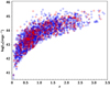 |
Fig. 1. Observed X-ray luminosity as a function of redshift. Blue and red symbols refer to the unabsorbed and absorbed sources, respectively. There is a selection bias against low-luminosity sources (log LX < 43 erg s−1) at high redshifts (z > 1). The effect of this incompleteness is taken into account (see Sect. 4.2 for details). |
Number of spectroscopic and photometric sources with SDSS, WISE, or Herschel photometry in our sample.
3. Analysis
In this section we describe the steps we followed in our analysis. The AGN host galaxy properties were estimated through SED fitting (Sect. 3.1). Section 3.2 describes the estimation of the X-ray properties of our sample and the methodology we followed to account for selection biases.
3.1. Host galaxy properties
The SFR and M* were estimated using version 0.12 of the Code Investigating GALaxy Emission (CIGALE; Burgarella et al. 2005; Noll et al. 2009; Boquien et al. 2019). The emission associated with AGN is modelled using the Fritz et al. (2006) library, as described in Ciesla et al. (2015). This allows us to disentangle the AGN IR emission from the IR emission of the host galaxy and derive more accurate SFR measurements. Sources with reduced χ2 > 5 have been excluded from our analysis. For more details on the SED fitting, the models used, and their parameter values, see Masoura et al. (2018).
Masoura et al. (2018; see their Fig. 7) found that the average SFR of AGN host galaxies presents an evolution with stellar mass and redshift that is similar to that of star-forming systems (e.g., Brinchmann et al. 2004; Elbaz et al. 2007; Daddi et al. 2007; Magdis et al. 2010; Salmon et al. 2015; Schreiber et al. 2015). To account for the evolution of the MS, we follow their approach (see also e.g., Bernhard et al. 2019), and make use of the SFRnorm parameter to examine whether the AGN type plays a systematic role in deviations (or dispersion) around it. This quantity is equal to the observed SFR, divided by the expected SFR at a given M* and redshift (SFRsnorm = SFR/SFRMS). To estimate the SFRMS we use Eq. (9) of Schreiber et al. (2015).
3.2. X-ray absorption
To classify the AGN as X-ray absorbed and unabsorbed we need to estimate their hydrogen column density. For that purpose we first apply a Bayesian method to calculate the HR and then infer the NH of each source. A detailed description of this process is provided below.
3.2.1. X-ray colours
The HR or X-ray colour is used to quantify and characterise weak sources and large samples. To reduce the drawbacks of the classical definition (e.g., Gaussian assumption for the error propagation of counts for faint sources with a significant background, background subtraction), we apply the Bayesian Estimation of Hardness Ratios code (BEHR; Park et al. 2006). This method applies a Bayesian approach to account for the Poissonian nature of the observations. For the estimations we use the number of photons in the soft (0.5−2.0 keV) and the hard (2.0−8.0 keV) bands, provided in the Liu et al. (2016) catalogue. The hardness ratio calculations are based on the equation
 (1)
(1)
where S and H are the counts in the soft and the hard band, respectively.
3.2.2. Hydrogen column density
The NH values for all the sources in our sample are estimated using the calculated HRs. The Portable, Interactive Multi-Mission Simulator (PIMMS; Mukai 1993) tool is used to create a grid of HR and NH values and to convert the HR values from BEHR into NH. PIMMs is also used to estimate the correction factor that is applied for the calculation of the intrinsic fluxes of our sources (see next paragraph). In our calculations we assumed that the power law X-ray spectrum has a fixed photon index (Γ) of 1.8. The value of galactic NH used is log  . The AGN sample is split into X-ray absorbed and unabsorbed sources using a NH cut at log
  . This value has been used in a number of previous studies since it provides good agreement between the X-ray and optical classification of type 1 and 2 AGNs (e.g., Merloni et al. 2014; Masoura et al. 2020). Figure 2 presents the distribution of the hydrogen column density for the examined sources. Its bimodal nature was also observed in previous works (e.g., Civano et al. 2016; Stemo et al. 2020).
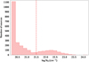 |
Fig. 2. Hydrogen column density (NH) distribution of the AGN sample. The vertical dashed line presents the NH cut applied in our analysis to split the sources into absorbed and unabsorbed. |
Having estimated NH, we compute the correction factor, defined as fint/fabs, where fabs is the absorbed flux and fint the intrinsic flux. The latter is estimated using PIMMS and assuming an unabsorbed power law with Γ = 1.8. Then, each observed X-ray luminosity is corrected using this factor to estimate the intrinsic X-ray luminosity. Figure 3 presents the distribution of redshift (left panel) and intrinsic X-ray luminosity (right panel) of absorbed (red line) and unabsorbed (blue line) AGNs. We note that the distributions of the two AGN subsamples are similar. This can be explained by the low X-ray absorption limit we adopt in our analysis. Adoption of a higher NH cut (log  ), results in different redshift and X-ray luminosity distributions between absorbed and unabsorbed sources, in agreement with the predictions of X-ray luminosity function studies (e.g., Aird et al. 2015).
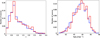 |
Fig. 3. Left: redshift distribution of the examined sample. Right: intrinsic X-ray luminosity distribution of the examined sample. The blue and red histograms refer to the unabsorbed and absorbed sources, respectively. Both histograms have been normalised to the total number of sources. |
4. Results and discussion
In this section we present our main results and compare them with previous studies. Specifically, we examine whether absorbed and unabsorbed AGNs have different host galaxy properties and whether the SFR–LX relation changes with absorption.
4.1. Host galaxy properties of absorbed and unabsorbed AGN
As presented in Fig. 3, the redshift and LX distributions of X-ray absorbed and unabsorbed classified AGN in our sample are similar. However, we account for the small differences between them to facilitate a better comparison of the host galaxy properties of the two populations. For that purpose we join the redshift distributions of the two populations and normalise each one by the total number of sources in each redshift bin (bin size of 0.1). We repeat the same process for the LX distributions of the two subsamples (bin size of 0.2 dex). This procedure provides us with the probability density function (PDF) in this 2D parameter space (i.e. redshift and LX space). Then we use the redshift and LX of each source to weigh it based on the estimated PDF (see also Mendez et al. 2016; Mountrichas et al. 2016). This correction method is similar to that applied in previous studies (e.g., Zou et al. 2019) and allows a fair comparison with their results. Additionally, each source is weighted based on the statistical significance of its stellar mass and SFR measurements (see next sections for details).
4.1.1. Stellar mass distribution
Stellar mass estimations for AGNs may suffer from large uncertainties, in particular in the case of unabsorbed sources. The AGN emission can outshine the optical emission of the host galaxy, thus rendering stellar mass calculations uncertain. The median stellar mass measurements and the median uncertainties, estimated by CIGALE are 10.6 ± 0.4 and 10.9 ± 0.6 for unabsorbed and absorbed AGNs, respectively. Restricting our sample to the most X-ray luminous (LX ≥ 1044 erg s−1) unabsorbed AGNs (∼20% of our total sample) gives 11.1 ± 0.8. Figure 4 presents the distributions of stellar mass uncertainties for absorbed (red shaded area) and unabsorbed (blue line) AGN. The two populations have similar distributions; the bulk of the measurements have errors ≤0.5−0.6 dex. We chose not to exclude sources with large stellar mass errors to avoid reducing the size of the dataset. Instead, we account for the M* uncertainties by estimating the significance (value/uncertainty; σ) of each stellar mass measurement, and weigh each source based on its sigma value (in addition to the weight presented in the previous paragraph). We confirm that excluding the sources that have stellar mass uncertainties larger than 0.6 dex (∼25% of unabsorbed and ∼33% of absorbed AGN) from our analysis does not change our results and conclusions compared to those presented using the weighting method described above.
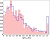 |
Fig. 4. Distributions of the error of the log M* for absorbed (red shaded histogram) and unabsorbed (blue line) AGNs. The two populations have similar error distributions; the bulk of the measurements have errors ≤0.5−0.6 dex. |
Figure 5 presents the distribution of M* for both absorbed and unabsorbed AGNs in bins of 0.2 dex. We apply a two-sample Kolmogorov–Smirnov test (KS-test) to examine whether the two distributions differ. The KS-test reveals that the distributions are similar for both AGN populations (p-value = 0.72). We also split the AGN sample into low- and high-redshift subsamples, using a redshift cut at z = 1.0 and repeat the process. The KS-test shows no statistically significant difference of the M* distribution of absorbed and unabsorbed sources at any redshift. Specifically, at z < 1.0 the KS-test gives p = 0.82, and at z > 1.0 it gives p = 0.39. Our findings are in agreement with Merloni et al. (2014) who used 1310 X-ray selected AGNs from the XMM-COSMOS survey with redshift range 0.3 < z < 3.5. In that study the X-ray population was split into obscured and unobscured AGN using the same NH cut that is applied in our analysis (NH = 1021.5 cm−2). They found no remarkable differences between the mean M* of obscured and unobscured AGNs. On the other hand, Lanzuisi et al. (2017) used approximately 700 X-ray selected AGNs in the COSMOS field in the redshift range 0.1 < z < 4, and found that unobscured AGNs tend to have lower M* than obscured sources. However, they considered as X-ray absorbed sources with NH > 1022 cm−2. To be consistent with Lanzuisi et al. (2017), we apply the KS-test adopting the same NH with them. The estimated p-value, although reduced to 0.56, still indicates that the M* distribution is similar for the two AGN populations. Furthermore, Zou et al. (2019) used 2463 X-ray selected AGNs in the COSMOS field, and found that unobscured AGNs tend to have lower M* than their obscured counterparts. However, in their analysis they divided their sample into type 1 and type 2 AGNs based on their optical spectra, morphologies, and variability. Thus, the disagreement with our results could be attributed to the different method applied in the characterisation of a source as obscured or unobscured.
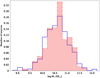 |
Fig. 5. Stellar mass distributions. The blue and red histograms refer to the unabsorbed and absorbed sources, respectively. The histograms have been normalised to the total number of sources. Based on the KS-test (p-value = 0.72), the two AGN populations have similar M* distributions. |
4.1.2. Star formation rate distribution
The left panel of Fig. 6 presents the distributions of the SFR, for both absorbed and unabsorbed AGNs, in bins of 0.3 dex for the total sample. Each source is weighted based on its X-ray luminosity and redshift and on the sigma value of its SFR measurement. Application of the two-sample KS-test reveals that the SFR distributions are similar for both AGN populations, with a p-value equal to 0.95. This is also the case when we split the AGN sample into low- and high-redshift subsamples, using a redshift cut at z = 1.0 (for z < 1.0, p = 0.99, and for z > 1.0, p = 0.86). In the right panel, we present the SFR distributions only for those AGNs that have available Herschel photometry. The results are similar to those for the full sample, i.e. the SFR distributions of X-ray absorbed and unabsorbed AGN present no significant differences (p-value = 0.86). Further restricting the sample to those sources with signal-to-noise ratios greater than 3 for the SPIRE bands (216 AGNs) does not change the results.
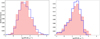 |
Fig. 6. Star formation rate distribution. The blue and red histograms refer to the unabsorbed and absorbed sources, respectively. The histograms have been normalised to the total number of sources. Left: distributions for the total number of sources. The two populations have similar SFR distributions (p-value = 0.95). Right: distributions for the 1276 AGNs with Herschel photometry available. The X-ray absorbed and unabsorbed AGNs have similar SFR distributions (p-value = 0.86). |
Our findings agree with most previous studies (Merloni et al. 2014; Lanzuisi et al. 2017; Zou et al. 2019). On the other hand, Chen et al. (2015) used AGNs from the Böotes field and claimed that type 2 sources have higher IR star formation luminosities (a proxy of star formation) than type 1, by a factor of ∼2. However, their dataset consists of mid-IR selected, luminous quasars. Moreover, they divide their sample into type 1 and type 2 AGNs using optical and mid-IR colour criteria R − [4.5] = 6.1 (e.g., Hickox et al. 2007), where R and [4.5] are the Vega magnitudes in the R and IRAC 4.5 μm bands, respectively.
4.1.3. Normalised star formation rate distribution
We calculate the SFRnorm to take into account the evolution of SFR with stellar mass and redshift (see Sect. 3.1). The distribution of SFRnorm of absorbed and unabsorbed AGN, in bins of 0.2 dex, is presented in Fig. 7. Each source is weighted based on its redshift and luminosity, as described in Sect. 4.1, and is also based on the significance of its stellar mass and star formation rate measurement. The KS-test results in a p-value equal to 0.71, i.e. the two populations have similar SFRnorm distributions. We note that both distributions are bimodal. Further investigation reveals that, for the absorbed and the unabsorbed sources, the first peak is due to low-redshift systems (mean z ≈ 0.7), while the second peak is due to AGNs that lie at high redshifts (mean z ≈ 1.5). This may suggest evolution of the SFRnorm with redshift. To investigate this scenario further, we split the AGN sample into two redshift bins, at z = 1.2. The SFRnorm distributions are presented in Fig. 8. The results confirm that the SFRnorm distribution peaks at different values at low and high redshifts. AGNs in the lower redshift bin have SFRs comparable with galaxies on the star-forming main sequence (log SFRnorm = 0), whereas AGNs at higher redshift have enhanced SFRs compared to galaxies on the main sequence. We discuss this in more detail in the next section.
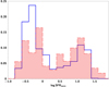 |
Fig. 7. Normalised star formation rate distribution. The blue and red histograms refer to the unabsorbed and absorbed sources, respectively. The histogram has been normalised to the total number of sources. The two populations have similar normalised SFR distributions (p-value = 0.71). Both distributions are bimodal. |
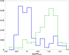 |
Fig. 8. Normalised star formation rate distribution for sources at z < 1.2 (blue line) and at z > 1.2 (green dashed line). The histogram has been normalised to the total number of sources. The AGNs in the lower redshift bin have SFRs comparable with galaxies on the star-forming main sequence (log SFRnorm = 0), whereas AGNs at higher redshift have enhanced SFRs compared to galaxies on the main sequence. This suggests evolution of the SFRnorm with redshift (see text for details). |
Bernhard et al. (2019) examined the SFR distribution of X-ray AGNs, taking into consideration its evolution with M* and redshift. Specifically, they used X-ray sources in the COSMOS field and investigated the SFRnorm distribution as a function of LX. Based on their analysis, more powerful AGNs present a narrower SFRnorm distribution that peaks close to that of the MS galaxies. Their sample consists of AGNs at intermediate redshifts (i.e. 0.8 < z < 1.2). Based on the mean redshift values of the systems contained in the two peaks of our SFRnorm distributions presented above, this would place their sources between our two peaks and close to the SFR of MS galaxies. Furthermore, the Bernhard et al. (2019) sample spans a narrower LX range and lacks sources at low LX, and in particular at high LX, compared to the sample used in our analysis (see our Fig. 1 and their Fig. 1). There are only ∼500 AGNs in our dataset that are within the redshift and luminosity range of Bernhard et al. (2019) Further restricting the sample to only obscured sources, in accordance with Bernhard et al. (2019), results in fewer than 200 sources. Applying their luminosity cut (LX = 2 × 1043 erg s−1) we divide AGNs into high- and low-luminosity systems. We note that there are less than 30 low-luminosity sources in our sample. The SFRnorm distribution of high- and low-LX AGNs (green and blue, respectively) is presented in Fig. 9. High-luminosity AGNs still present a two-peaked SFRnorm. We note, however, that although we have matched the redshift and LX range with that of Bernhard et al. (2019), the LX distributions of the two datasets are still different. Nevertheless, the two results agree that higher X-ray luminosity AGNs exhibit higher SFRnorm values. We conclude that the different results between our study and that of Bernhard et al. (2019) could be due to the different LX, redshift plane probed by the samples of the two studies, and in particular the different luminosity distributions between the two datasets.
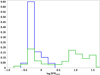 |
Fig. 9. SFRnorm distribution for low (LX < 2 × 1043 erg s−1, blue line) and high (LX > 2 × 1043 erg s−1, green line) X-ray luminosities. Redshift and LX range have been restricted to match that of Bernhard et al. (2019). We only present measurements for the X-ray absorbed AGNs. |
4.2. SFRnorm − LX correlation for different AGN types
In this section we study the effect of obscuration on the SFR–LX relation. To account for the evolution of SFR with stellar mass and redshift (see also Sect. 3.1) we plot SFRnorm estimations versus LX.
Luminous sources are observed within a larger volume compared to their faint counterparts in flux limited surveys (Fig. 1). This introduces a selection bias to our analysis. To account for this effect we adopt the  correction method (Akylas et al. 2006; Page & Carrera 2000). Specifically, we estimate the maximum available volume that can be observed for each source of a given LX using the equation
 (2)
(2)
where Ω(f) is the value of the sensitivity curve at a given flux, corresponding to a source at a redshift z with observed luminosity LX, and zmax is the maximum redshift at which the source can be observed at the flux limit of the survey. The area curve used in our calculations is presented in Liu et al. (2016; see their Fig. 3). Therefore, each source is weighted by the  value, depending on their LX and redshift. An additional weight is also considered, based on the sigma value of the M* and SFR measurements.
In Fig. 10 (left panel), we present our measurements in LX bins, for absorbed and unabsorbed AGNs, in bins of size 0.5 dex. Median SFR and LX values are presented. The error bars represent the 1σ dispersion of each bin, i.e. they do not take into account the errors of the individual SFR and stellar mass measurements. The number of sources varies in each bin, but our results are not sensitive to the choice of the number and size of bins. Based on our findings, both X-ray absorbed and unabsorbed AGNs present a similar SFR–LX relation at all X-ray luminosities spanned by our sample. We present our measurements in SFRnorm bins (bin size 0.5 dex, right panel of Fig. 10). Previous studies have also found that different binning affects the observed trends (e.g., Lanzuisi et al. 2017; Hickox et al. 2014). However, further examination of the underlying reasons that could be responsible for this effect are beyond the scope of this paper. Based on our findings, X-ray absorption does not play a significant role in the SFR–LX relation, regardless of whether our measurements are binned in LX or SFR bins.
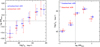 |
Fig. 10. Left: SFRnorm − LX correlation in LX bins, for absorbed and unabsorbed sources. Based on our measurements the AGN enhances the SFR of the host galaxy at all X-ray luminosities spanned by our sample, regardless of whether the source is X-ray absorbed or not. Right: SFRnorm − LX correlation in SFRnorm bins, for absorbed and unabsorbed sources (Masoura et al. 2018). Absorbed and unabsorbed sources approximately follow the same trend. In both plots red and blue triangles refer to the absorbed and unabsorbed sources, respectively. The dashed line corresponds to the star-forming main sequence. Median SFR and LX values are presented in both panels. The error bars represent the 1σ dispersion of each bin. Based on our measurements, the SFRnorm − LX correlation is similar for different AGN types. |
Additionally, we examine if and how the redshift range affects our estimations. The NH values estimated in Sect. 3.2.2 could be considered less secure as we move to higher redshifts because the absorption redshifts out of the soft X-ray band in the observed frame. Moreover, as shown in Fig. 1, our sample lacks low-luminosity sources at high redshifts (z > 1). Thus, in Fig. 11 we plot SFRnorm − LX for the whole sample (left), and the absorbed (middle) and unabsorbed (right) subsamples using three redshift bins (z < 0.5, 0.5 < z < 1.2, and z > 1.2). Results are presented in LX bins. The size of the bins varies from 0.25 to 0.5 dex depending on the available number of sources in each subsample. Median SFR and LX values are shown. The error bars represent the 1σ dispersion of each bin. For X-ray absorbed sources we find no difference in the dependence of the SFR on the AGN power, at all redshifts. However, X-ray unabsorbed sources at high redshift (z > 1.2) present a flat SFRnorm − LX relation.
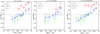 |
Fig. 11. SFRnorm − LX correlation in LX bins, for different redshift intervals (z < 0.5, 0.5 < z < 1.2 and z > 1.2). Left, middle, and right panels: full sample, absorbed population, and unabsorbed population, respectively. The dashed line corresponds to the star-forming main sequence. Trends are similar in all redshift bins. Median SFR and LX values are presented. The error bars represent the 1σ dispersion of each bin. |
Our results also show the evolution of the SFRnorm with redshift for the full sample and for the X-ray absorbed and unabsorbed AGNs (see also Fig. 7). This evolution does not appear statistically significant for redshifts below z < 1.2 (≤1σ), but its statistical significance increases (≈2−2.5σ, estimated by adding in quadrature the errors of the bins) between the lowest and highest of our redshift bins. This result suggests that as we move to higher redshifts, galaxies that host AGNs tend to have a greater increase in their SFRs compared to star-forming galaxies. At higher redshifts, galaxy mergers are more common than at low redshifts (e.g., Lin et al. 2008). These mergers can drive gas towards the centre of galaxies leading to enhanced star formation and AGN activity when some of this gas is deposited on the central black hole, as has been shown by both theoretical (e.g., Barnes & Hernquist 1992; Hopkins & Hernquist 2006; Hopkins et al. 2008) and observational studies (e.g., Hung et al. 2013). Galaxies in the late stages of a merger have increased SFR and AGN activity (e.g., Stierwalt et al. 2013). Therefore, our findings that the SFRs of AGNs increase more rapidly with redshift compared to non-AGN systems may indicate that AGNs are observed at a late(r) evolutionary merger stage when the central black hole has been activated and the SFR of the galaxy is at its peak. Alternatively, the enhanced SFRs of AGNs compared to normal galaxies at high redshifts may be due to the different AGN fueling processes and different star formation trigger mechanisms at high and low redshifts (e.g., mergers versus disc instabilities Somerville et al. 2001; Kereš et al. 2005).
Mullaney et al. (2015), used X-ray AGNs from Chandra Deep Field South and Chandra Deep Field North, and found no evolution of SFRnorm with redshift. However, their sample is extracted from narrow fields and therefore does not probe as many luminous sources as those detected in XXL, nor ones that are as high. Based on our results (see Fig. 11), the SFRnorm evolution becomes apparent at high X-ray luminosities (LX ≥ 1044 erg s−1), which are rare in deep fields.
4.3. Star formation as a function of X-ray absorption
Star formation rate is a galaxy wide quantity, while X-ray obscuration occurs in the regime around the black hole. However, it has been claimed that obscuration can also occur on galaxy scale (e.g., Fabbiano et al. 2017; Malizia et al. 2020). In this case the two properties may be correlated. Thus, in this part of our analysis we investigate whether there is a dependence of SFR on the X-ray absorption.
Rosario et al. (2012) used a sample of AGNs from the GOODS-South, GOODS-North, and COSMOS fields, spanning the redshifts 0.2 < z < 2.5. The NH values were estimated using either spectral fits for the X-ray sources with sufficient counts or scalings based on hardness ratios for faint X-ray sources. They found a mild dependence between the mean far-IR luminosity (SFR proxy) and the X-ray obscuring column (NH). On the other hand, Rovilos et al. (2012) used AGNs from the 3 Ms XMM-Newton survey with z ≃ 0.5−4 and reported that there is no correlation between SFR and NH. They claimed that the absorption is likely to be linked to the nuclear region rather than the host galaxy. Their findings were recently confirmed by Stemo et al. (2020). This group used X-ray and/or IR selected AGNs (Spitzer and Chandra data) and composed a sample of 2585 sources with redshifts in the range 0.2 < z < 2.5. They compiled data from the GEMS, COSMOS, GOODS, and AEGIS surveys. They used extinction parameter, EB − V, and values estimated through SED fitting to infer the NH values, using a conversion factor of EB − V/NH = 1.80 ± 0.15 × 10⁻²³. Based on their findings the relation between the SFR and NH is flat up to z = 2.5. According to their interpretation, this behaviour indicates a difference in fuelling processes or timescales between SMBH growth and host galaxy star formation.
In Fig. 12, we plot star formation as a function of NH for our X-ray AGN sources. All sources are weighted based on the  method, and on the significance of the SFR measurements. Median SFR and NH values are presented. The error bars represent the 1σ dispersion of each bin, i.e. they do not take into account the errors of the individual SFR calculations. Measurements are binned in NH, with bin size of 0.5 dex. We detect a flat relation between the two parameters, at all redshifts spanned by our sample. Our results are in agreement with previous works that have used AGNs with similar X-ray properties (i.e. low to moderate levels of X-ray absorption). We note, however, that this result may not hold at higher NH values.
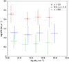 |
Fig. 12. Star formation rate as a function of NH. The sample is split into redshift bins. The green, blue, and red symbols refer to z < 0.5, 0.5 < z < 1.2, and z > 1.2, respectively. Median SFRs and NH values are presented. The error bars represent the 1σ dispersion of each bin. Measurements reveal a flat relation between star formation and X-ray absorption at all redshift ranges. |
5. Summary
In this study we used 3213 AGNs from the XMM-XXL northern field to investigate the relation of the AGN type with the host galaxy properties. About 60% of our sources had available spectroscopic redshift, while for the remaining sources we used photometric redshifts estimated through a machine learning technique (TPZ). The host galaxy properties, SFR, and stellar mass were estimated via the SED fitting code CIGALE. A statistical method based on Bayesian statistics (BEHR) was applied to derive the HRs for the examined sample. AGNs with NH > 1021.5 cm−2 were considered to be absorbed.
First, we studied whether there is a connection between AGN type and the properties of the host galaxy. We estimated the SFR and M* distributions of both X-ray absorbed and unabsorbed AGN. A KS-test revealed that the galaxy properties of the two AGN populations are similar.
Next, we disentangled the effects of M* and redshift on SFR and examined the SFR–LX relation, as a function of AGN type. We find that the SFR–LX relation is similar for absorbed and unabsorbed AGN at all redshifts spanned by our sample. This behaviour indicates that the interplay between the AGN and its host galaxy is independent of the obscuration.
Finally, we explored whether the SFR varies as a function of the absorbing column density. Our results show that there is no relation between the two, suggesting that either the two processes take place on different scales or that it does not relate with the SFR of the host galaxy, even if absorption extends to galactic scales.
Overall, our results suggest that there is no connection between X-ray absorption and the properties of the host galaxy nor the AGN-galaxy co-evolution. This provides support to the unification model, i.e. X-ray absorption seems to be an inclination effect and not a phase in the lifetime of the AGN. We note, however, that in our analysis we have adopted a rather low X-ray absorption limit. XMM-XXL is a shallow exposure field, and thus there is only a small number of heavily absorbed sources (NH ∼ 1023 cm−2). Future surveys that will provide larger datasets of obscured AGNs and/or with higher column densities (eROSITA, ATHENA) will allow us to study whether this picture holds also for the most heavily absorbed AGNs.
The Herschel Extragalactic Legacy Project (HELP, http://herschel.sussex.ac.uk/) is a European funded project to analyse all the cosmological fields observed with the Herschel satellite. HELP data products are accessible on HeDaM (http://hedam.lam.fr/HELP/).
Acknowledgments
The authors thank the anonymous referee for their detailed report that improved the quality of the paper. The authors also thank Dr. A. Akylas for his help in estimating the X-ray properties of the sample and Prof. P. Papadopoulos for a detailed reading of the manuscript and useful comments. VAM and IG acknowledge support of this work by the PROTEAS II project (MIS 5002515), which is implemented under the “Reinforcement of the Research and Innovation Infrastructure” action, funded by the “Competitiveness, Entrepreneurship and Innovation” operational programme (NSRF 2014-2020) and co-financed by Greece and the European Union (European Regional Development Fund). This research is co-financed by Greece and the European Union (European Social Fund-ESF) through the Operational Programme “Human Resources Development, Education and Lifelong Learning 2014–2020” in the context of the project “Anatomy of galaxies: their stellar and dust content though cosmic time” (MIS 5052455). GM acknowledges support by the Agencia Estatal de Investigación, Unidad de Excelencia María de Maeztu, ref. MDM-2017-0765. XXL is an international project based around an XXM Very Large Programme surveying two 25 deg2 extragalactic fields at a depth of ∼6 × 10⁻¹⁵ erg cm−2 s−1 in the [0.5−2] keV band for point-like sources. The XXL website is http://irfu.cea.fr/xxl/. Multi-band information and spectroscopic follow-up of the X-ray sources are obtained through a number of survey programmes, summarised at http://xxlmultiwave.pbworks.com/. This research has made use of data obtained from the 3XMM XMM-Newton serendipitous source catalogue compiled by the 10 institutes of the XMM-Newton Survey Science Centre selected by ESA. This work is based on observations made with XMM-Newton, an ESA science mission with instruments and contributions directly funded by ESA Member States and NASA. Funding for the Sloan Digital Sky Survey IV has been provided by the Alfred P. Sloan Foundation, the US Department of Energy Office of Science, and the Participating Institutions. SDSS-IV acknowledges support and resources from the Center for High-Performance Computing at the University of Utah. The SDSS website is www.sdss.org. SDSS-IV is managed by the Astrophysical Research Consortium for the Participating Institutions of the SDSS Collaboration including the Brazilian Participation Group, the Carnegie Institution for Science, Carnegie Mellon University, the Chilean Participation Group, the French Participation Group, Harvard-Smithsonian Center for Astrophysics, Instituto de Astrofísica de Canarias, The Johns Hopkins University, Kavli Institute for the Physics and Mathematics of the Universe (IPMU)/University of Tokyo, Lawrence Berkeley National Laboratory, Leibniz Institut für Astrophysik Potsdam (AIP), Max-Planck-Institut für Astronomie (MPIA Heidelberg), Max-Planck-Institut für Astrophysik (MPA Garching), Max-Planck-Institut für Extraterrestrische Physik (MPE), National Astronomical Observatories of China, New Mexico State University, New York University, University of Notre Dame, Observatário Nacional/MCTI, The Ohio State University, Pennsylvania State University, Shanghai Astronomical Observatory, United Kingdom Participation Group, Universidad Nacional Autónoma de México, University of Arizona, University of Colorado Boulder, University of Oxford, University of Portsmouth, University of Utah, University of Virginia, University of Washington, University of Wisconsin, Vanderbilt University, and Yale University. This publication makes use of data products from the Wide-field Infrared Survey Explorer, which is a joint project of the University of California, Los Angeles, and the Jet Propulsion Laboratory/California Institute of Technology, funded by the National Aeronautics and Space Administration. The VISTA Data Flow System pipeline processing and science archive are described in Irwin et al. (2004), Hambly et al. (2008), and Cross et al. (2012). Based on observations obtained as part of the VISTA Hemisphere Survey, ESO Program, 179.A-2010 (PI: McMahon). We have used data from the 3rd data release.
References
- Aird, J., Coil, A. L., Georgakakis, A., et al. 2015, MNRAS, 451, 1892 [NASA ADS] [CrossRef] [Google Scholar]
- Aird, J., Coil, A. L., & Georgakakis, A. 2016, MNRAS, 465, 3390 [Google Scholar]
- Aird, J., Coil, A. L., & Georgakakis, A. 2019, MNRAS, 484, 4360 [NASA ADS] [CrossRef] [Google Scholar]
- Akylas, A., & Georgantopoulos, I. 2008, A&A, 479, 735 [NASA ADS] [CrossRef] [EDP Sciences] [Google Scholar]
- Akylas, A., Georgantopoulos, I., Georgakakis, A., Kitsionas, S., & Hatziminaoglou, E. 2006, A&A, 459, 693 [NASA ADS] [CrossRef] [EDP Sciences] [Google Scholar]
- Alexander, D. M., & Hickox, R. C. 2012, New Astron. Rev., 56, 93 [NASA ADS] [CrossRef] [Google Scholar]
- Antonucci, R. 1993, ARA&A, 31, 473 [Google Scholar]
- Barnes, J. E., & Hernquist, L. 1992, ARA&A, 30, 705 [NASA ADS] [CrossRef] [Google Scholar]
- Barvainis, R. 1987, ApJ, 320, 537 [NASA ADS] [CrossRef] [Google Scholar]
- Bernhard, E., Grimmett, L. P., Mullaney, J. R., et al. 2019, MNRAS, 483, L52 [CrossRef] [Google Scholar]
- Boquien, M., Burgarella, D., Roehlly, Y., et al. 2019, A&A, 622, A103 [NASA ADS] [CrossRef] [EDP Sciences] [Google Scholar]
- Bournaud, F., Elmegreen, B. G., & Elmegreen, D. M. 2007, ApJ, 670, 237 [Google Scholar]
- Brinchmann, J., Charlot, S., White, S. D. M., et al. 2004, MNRAS, 351, 1151 [NASA ADS] [CrossRef] [Google Scholar]
- Brown, A., Nayyeri, H., Cooray, A., et al. 2019, ApJ, 871, 87 [CrossRef] [Google Scholar]
- Buchner, J., & Bauer, F. E. 2016, MNRAS, 465, 4348 [NASA ADS] [CrossRef] [Google Scholar]
- Burgarella, D., Buat, V., & Iglesias-Páramo, J. 2005, MNRAS, 360, 1413 [Google Scholar]
- Carrasco Kind, M., & Brunner, R. J. 2013, MNRAS, 432, 1483 [NASA ADS] [CrossRef] [Google Scholar]
- Chen, C.-T. J., Hickox, R. C., Alberts, S., et al. 2013, ApJ, 773, 3 [NASA ADS] [CrossRef] [Google Scholar]
- Chen, C.-T. J., Hickox, R. C., Alberts, S., et al. 2015, ApJ, 802, 50 [NASA ADS] [CrossRef] [Google Scholar]
- Ciesla, L., Charmandaris, V., Georgakakis, A., et al. 2015, A&A, 576, A10 [NASA ADS] [CrossRef] [EDP Sciences] [Google Scholar]
- Ciotti, L., & Ostriker, J. P. 1997, ApJ, 487, L105 [NASA ADS] [CrossRef] [Google Scholar]
- Ciotti, L., & Ostriker, J. P. 2001, ApJ, 551, 131 [NASA ADS] [CrossRef] [Google Scholar]
- Circosta, C., Vignali, C., Gilli, R., et al. 2019, A&A, 623, A172 [NASA ADS] [CrossRef] [EDP Sciences] [Google Scholar]
- Civano, F., Marchesi, S., Comastri, A., et al. 2016, ApJ, 819, 62 [Google Scholar]
- Cross, N. J. G., Collins, R. S., Mann, R. G., et al. 2012, A&A, 548, A119 [NASA ADS] [CrossRef] [EDP Sciences] [Google Scholar]
- Daddi, E., Dickinson, M., Morrison, G., et al. 2007, ApJ, 670, 156 [NASA ADS] [CrossRef] [Google Scholar]
- Di Matteo, T., Springel, V., & Hernquist, L. 2005, Nature, 433, 604 [NASA ADS] [CrossRef] [PubMed] [Google Scholar]
- Di Matteo, T., Colberg, J., Springel, V., Hernquist, L., & Sijacki, D. 2008, ApJ, 676, 33 [NASA ADS] [CrossRef] [Google Scholar]
- Draine, B. T. 2003, ApJ, 598, 1026 [Google Scholar]
- Eales, S., Dunne, L., Clements, D., et al. 2010, PASP, 122, 499 [NASA ADS] [CrossRef] [Google Scholar]
- Elbaz, D., Daddi, E., Borgne, D. L., et al. 2007, A&A, 468, 33 [NASA ADS] [CrossRef] [EDP Sciences] [Google Scholar]
- Elvis, M., Wilkes, B. J., McDowell, J. C., et al. 1994, ApJS, 95, 1 [Google Scholar]
- Fabbiano, G., Elvis, M., Paggi, A., et al. 2017, ApJ, 842, L4 [NASA ADS] [CrossRef] [Google Scholar]
- Fabian, A. C. 1999, MNRAS, 308, L39 [NASA ADS] [CrossRef] [Google Scholar]
- Fanidakis, N., Baugh, C. M., Benson, A. J., et al. 2011, MNRAS, 410, 53 [NASA ADS] [CrossRef] [Google Scholar]
- Ferrarese, L., & Merritt, D. 2000, ApJ, 539, 9 [NASA ADS] [CrossRef] [Google Scholar]
- Florez, J., Jogee, S., Sherman, S., et al. 2020, MNRAS, 497, 3273 [NASA ADS] [CrossRef] [Google Scholar]
- Fritz, J., Franceschini, A., & Hatziminaoglou, E. 2006, MNRAS, 166, 767 [NASA ADS] [CrossRef] [Google Scholar]
- Georgakakis, A., & Nandra, K. 2011, MNRAS, 414, 992 [NASA ADS] [CrossRef] [Google Scholar]
- Georgakakis, A., Salvato, M., Liu, Z., et al. 2017, MNRAS, 469, 3232 [NASA ADS] [CrossRef] [Google Scholar]
- Gilli, R., Comastri, A., & Hasinger, G. 2007, A&A, 463, 79 [NASA ADS] [CrossRef] [EDP Sciences] [Google Scholar]
- Grimmett, L. P., Mullaney, J. R., Bernhard, E. P., et al. 2020, MNRAS, 495, 1392 [CrossRef] [Google Scholar]
- Hambly, N. C., Collins, R. S., Cross, N. J. G., et al. 2008, MNRAS, 384, 637 [NASA ADS] [CrossRef] [Google Scholar]
- Harrison, C. M., Alexander, D. M., Mullaney, J. R., et al. 2012, ApJ, 760, L15 [NASA ADS] [CrossRef] [Google Scholar]
- Hickox, R. C., & Alexander, D. M. 2018, ARA&A, 56, 625 [Google Scholar]
- Hickox, R. C., Jones, C., Forman, W. R., et al. 2007, ApJ, 671, 1365 [NASA ADS] [CrossRef] [Google Scholar]
- Hickox, R. C., Myers, A. D., Brodwin, M., et al. 2011, ApJ, 731, 117 [NASA ADS] [CrossRef] [Google Scholar]
- Hickox, R. C., Mullaney, J. R., Alexander, D. M., et al. 2014, ApJ, 782, 11 [NASA ADS] [CrossRef] [Google Scholar]
- Hopkins, P. F., & Hernquist, L. 2006, ApJS, 166, 1 [NASA ADS] [CrossRef] [Google Scholar]
- Hopkins, P. F., Hernquist, L., Cox, T. J., et al. 2006, ApJ, 639, 700 [NASA ADS] [CrossRef] [Google Scholar]
- Hopkins, P. F., Hernquist, L., Cox, T. J., & Kereš, D. 2008, ApJS, 175, 356 [NASA ADS] [CrossRef] [Google Scholar]
- Hung, C.-L., Sanders, D. B., Casey, C. M., et al. 2013, ApJ, 778, 129 [NASA ADS] [CrossRef] [Google Scholar]
- Hurley, P. D., Oliver, S., Betancourt, M., et al. 2017, MNRAS, 464, 885 [NASA ADS] [CrossRef] [Google Scholar]
- Irwin, M. J., Lewis, J., Hodgkin, S., et al. 2004, Proc. SPIE, 5493, 411 [NASA ADS] [CrossRef] [Google Scholar]
- Kereš, D., Katz, N., Weinberg, D. H., & Dave, R. 2005, MNRAS, 363, 2 [NASA ADS] [CrossRef] [Google Scholar]
- Lanzuisi, G., Delvecchio, I., Berta, S., et al. 2017, A&A, 602, A123 [NASA ADS] [CrossRef] [EDP Sciences] [Google Scholar]
- Lin, L., Patton, D. R., Koo, D. C., et al. 2008, ApJ, 681, 232 [NASA ADS] [CrossRef] [Google Scholar]
- Liu, Z., Merloni, A., Georgakakis, A., et al. 2016, MNRAS, 459, 1602 [NASA ADS] [CrossRef] [Google Scholar]
- Lusso, E., & Risaliti, G. 2016, ApJ, 819, 154 [NASA ADS] [CrossRef] [Google Scholar]
- Lutz, D., Mainieri, V., Rafferty, D., et al. 2010, ApJ, 712, 1287 [NASA ADS] [CrossRef] [Google Scholar]
- Magdis, G. E., Rigopoulou, D., Huang, J.-S., & Fazio, G. G. 2010, MNRAS, 401, 1521 [NASA ADS] [CrossRef] [Google Scholar]
- Magorrian, J., Tremaine, S., Richstone, D., et al. 1998, AJ, 115, 2285 [Google Scholar]
- Maiolino, R., & Rieke, G. H. 1995, ApJ, 454, 95 [NASA ADS] [CrossRef] [Google Scholar]
- Maiolino, R., Ruiz, M., Rieke, G. H., & Papadopoulos, P. 1997, ApJ, 485, 552 [NASA ADS] [CrossRef] [Google Scholar]
- Malizia, A., Bassani, L., Stephen, J. B., Bazzano, A., & Ubertini, P. 2020, A&A, 639, A5 [CrossRef] [EDP Sciences] [Google Scholar]
- Malkan, M. A., Gorjian, V., & Tam, R. 1998, ApJS, 117, 25 [NASA ADS] [CrossRef] [Google Scholar]
- Masoura, V. A., Mountrichas, G., Georgantopoulos, I., et al. 2018, A&A, 618, A31 [NASA ADS] [CrossRef] [EDP Sciences] [Google Scholar]
- Masoura, V. A., Georgantopoulos, I., Mountrichas, G., et al. 2020, A&A, 638, A45 [CrossRef] [EDP Sciences] [Google Scholar]
- Matt, G. 2000, A&A, 355, L31 [NASA ADS] [Google Scholar]
- Mendez, A. J., Coil, A. L., Aird, J., et al. 2016, ApJ, 821, 55 [NASA ADS] [CrossRef] [Google Scholar]
- Menzel, M.-L., Merloni, A., Georgakakis, A., et al. 2016, MNRAS, 457, 110 [NASA ADS] [CrossRef] [Google Scholar]
- Merloni, A., Bongiorno, A., Brusa, M., et al. 2014, MNRAS, 437, 3550 [NASA ADS] [CrossRef] [Google Scholar]
- Mountrichas, G., Georgakakis, A., Menzel, M.-L., et al. 2016, MNRAS, 457, 4195 [NASA ADS] [CrossRef] [Google Scholar]
- Mountrichas, G., Georgantopoulos, I., Secrest, N. J., et al. 2017, MNRAS, 468, 3042 [NASA ADS] [CrossRef] [Google Scholar]
- Mukai, K. 1993, Legacy, 3, 21 [Google Scholar]
- Mullaney, J. R., Alexander, D. M., Aird, J., et al. 2015, MNRAS, 453, L83 [NASA ADS] [CrossRef] [Google Scholar]
- Netzer, H. 2015, ARA&A, 53, 365 [NASA ADS] [CrossRef] [Google Scholar]
- Noll, S., Burgarella, D., Giovannoli, E., et al. 2009, A&A, 507, 1793 [NASA ADS] [CrossRef] [EDP Sciences] [Google Scholar]
- Oliver, S. J., Bock, J., Altieri, B., et al. 2012, MNRAS, 424, 1614 [Google Scholar]
- Page, M. J., & Carrera, F. J. 2000, MNRAS, 311, 433 [NASA ADS] [CrossRef] [Google Scholar]
- Page, M. J., Symeonidis, M., Vieira, J. D., et al. 2012, Nature, 485, 213 [NASA ADS] [CrossRef] [Google Scholar]
- Park, T., Kashyap, V. L., Siemiginowska, A., et al. 2006, AJ, 652, 610 [NASA ADS] [CrossRef] [Google Scholar]
- Pierre, M., Pacaud, F., Adami, C., et al. 2016, A&A, 592, A1 [NASA ADS] [CrossRef] [EDP Sciences] [Google Scholar]
- Rodighiero, G., Brusa, M., Daddi, E., et al. 2015, ApJ, 800, L10 [CrossRef] [Google Scholar]
- Rosario, D. J., Santini, P., Lutz, D., et al. 2012, A&A, 545, 45 [NASA ADS] [CrossRef] [EDP Sciences] [Google Scholar]
- Rosario, D. J., Trakhtenbrot, B., Lutz, D., et al. 2013, A&A, 560, A72 [NASA ADS] [CrossRef] [EDP Sciences] [Google Scholar]
- Rovilos, E., & Georgantopoulos, I. 2007, A&A, 475, 115 [NASA ADS] [CrossRef] [EDP Sciences] [Google Scholar]
- Rovilos, E., Comastri, A., Gilli, R., et al. 2012, A&A, 546, 16 [NASA ADS] [CrossRef] [EDP Sciences] [Google Scholar]
- Ruiz, A., Corral, A., Mountrichas, G., & Georgantopoulos, I. 2018, A&A, 618, A52 [CrossRef] [EDP Sciences] [Google Scholar]
- Salmon, B., Papovich, C., Finkelstein, S. L., et al. 2015, ApJ, 799, 183 [NASA ADS] [CrossRef] [Google Scholar]
- Sanders, D. B., Phinney, E. S., Neugebauer, G., Soifer, B. T., & Matthews, K. 1989, ApJ, 347, 29 [NASA ADS] [CrossRef] [Google Scholar]
- Schmidt, M. 1968, ApJ, 151, 393 [NASA ADS] [CrossRef] [Google Scholar]
- Schreiber, C., Pannella, M., Elbaz, D., et al. 2015, A&A, 575, A74 [NASA ADS] [CrossRef] [EDP Sciences] [Google Scholar]
- Shirley, R., Roehlly, Y., Hurley, P. D., et al. 2019, MNRAS, 490, 634 [CrossRef] [Google Scholar]
- Somerville, R. S., Primack, J. R., & Faber, S. M. 2001, MNRAS, 320, 504 [NASA ADS] [CrossRef] [Google Scholar]
- Somerville, R. S., Hopkins, P. F., Cox, T. J., Robertson, B. E., & Hernquist, L. 2008, MNRAS, 391, 481 [NASA ADS] [CrossRef] [Google Scholar]
- Stanley, F., Harrison, C. M., Alexander, D. M., et al. 2015, MNRAS, 453, 591 [NASA ADS] [CrossRef] [Google Scholar]
- Stemo, A., Comerford, J. M., Barrows, R. S., et al. 2020, ApJ, 888, 78 [CrossRef] [Google Scholar]
- Stierwalt, S., Armus, L., Surace, J. A., et al. 2013, ApJS, 206, 1 [NASA ADS] [CrossRef] [Google Scholar]
- Sutherland, W., & Saunders, W. 1992, MNRAS, 259, 413 [NASA ADS] [CrossRef] [Google Scholar]
- Treister, E., Urry, C. M., Chatzichristou, E., et al. 2004, ApJ, 616, 123 [NASA ADS] [CrossRef] [Google Scholar]
- Treister, E., Urry, C. M., & Virani, S. 2009, ApJ, 696, 110 [NASA ADS] [CrossRef] [Google Scholar]
- Urry, C. M., & Padovani, P. 1995, PASP, 107, 803 [Google Scholar]
- Volonteri, M., Capelo, P. R., Netzer, H., et al. 2015a, MNRAS, 452, L6 [NASA ADS] [CrossRef] [Google Scholar]
- Volonteri, M., Capelo, P. R., Netzer, H., et al. 2015b, MNRAS, 449, 1470 [NASA ADS] [CrossRef] [Google Scholar]
- Zou, F., Yang, G., Brandt, W. N., & Xue, Y. 2019, ApJ, 878, 11 [CrossRef] [Google Scholar]
All Tables
Number of spectroscopic and photometric sources with SDSS, WISE, or Herschel photometry in our sample.
All Figures
|
Fig. 1. Observed X-ray luminosity as a function of redshift. Blue and red symbols refer to the unabsorbed and absorbed sources, respectively. There is a selection bias against low-luminosity sources (log LX < 43 erg s−1) at high redshifts (z > 1). The effect of this incompleteness is taken into account (see Sect. 4.2 for details). |
| In the text | |
|
Fig. 2. Hydrogen column density (NH) distribution of the AGN sample. The vertical dashed line presents the NH cut applied in our analysis to split the sources into absorbed and unabsorbed. |
| In the text | |
|
Fig. 3. Left: redshift distribution of the examined sample. Right: intrinsic X-ray luminosity distribution of the examined sample. The blue and red histograms refer to the unabsorbed and absorbed sources, respectively. Both histograms have been normalised to the total number of sources. |
| In the text | |
|
Fig. 4. Distributions of the error of the log M* for absorbed (red shaded histogram) and unabsorbed (blue line) AGNs. The two populations have similar error distributions; the bulk of the measurements have errors ≤0.5−0.6 dex. |
| In the text | |
|
Fig. 5. Stellar mass distributions. The blue and red histograms refer to the unabsorbed and absorbed sources, respectively. The histograms have been normalised to the total number of sources. Based on the KS-test (p-value = 0.72), the two AGN populations have similar M* distributions. |
| In the text | |
|
Fig. 6. Star formation rate distribution. The blue and red histograms refer to the unabsorbed and absorbed sources, respectively. The histograms have been normalised to the total number of sources. Left: distributions for the total number of sources. The two populations have similar SFR distributions (p-value = 0.95). Right: distributions for the 1276 AGNs with Herschel photometry available. The X-ray absorbed and unabsorbed AGNs have similar SFR distributions (p-value = 0.86). |
| In the text | |
|
Fig. 7. Normalised star formation rate distribution. The blue and red histograms refer to the unabsorbed and absorbed sources, respectively. The histogram has been normalised to the total number of sources. The two populations have similar normalised SFR distributions (p-value = 0.71). Both distributions are bimodal. |
| In the text | |
|
Fig. 8. Normalised star formation rate distribution for sources at z < 1.2 (blue line) and at z > 1.2 (green dashed line). The histogram has been normalised to the total number of sources. The AGNs in the lower redshift bin have SFRs comparable with galaxies on the star-forming main sequence (log SFRnorm = 0), whereas AGNs at higher redshift have enhanced SFRs compared to galaxies on the main sequence. This suggests evolution of the SFRnorm with redshift (see text for details). |
| In the text | |
|
Fig. 9. SFRnorm distribution for low (LX < 2 × 1043 erg s−1, blue line) and high (LX > 2 × 1043 erg s−1, green line) X-ray luminosities. Redshift and LX range have been restricted to match that of Bernhard et al. (2019). We only present measurements for the X-ray absorbed AGNs. |
| In the text | |
|
Fig. 10. Left: SFRnorm − LX correlation in LX bins, for absorbed and unabsorbed sources. Based on our measurements the AGN enhances the SFR of the host galaxy at all X-ray luminosities spanned by our sample, regardless of whether the source is X-ray absorbed or not. Right: SFRnorm − LX correlation in SFRnorm bins, for absorbed and unabsorbed sources (Masoura et al. 2018). Absorbed and unabsorbed sources approximately follow the same trend. In both plots red and blue triangles refer to the absorbed and unabsorbed sources, respectively. The dashed line corresponds to the star-forming main sequence. Median SFR and LX values are presented in both panels. The error bars represent the 1σ dispersion of each bin. Based on our measurements, the SFRnorm − LX correlation is similar for different AGN types. |
| In the text | |
|
Fig. 11. SFRnorm − LX correlation in LX bins, for different redshift intervals (z < 0.5, 0.5 < z < 1.2 and z > 1.2). Left, middle, and right panels: full sample, absorbed population, and unabsorbed population, respectively. The dashed line corresponds to the star-forming main sequence. Trends are similar in all redshift bins. Median SFR and LX values are presented. The error bars represent the 1σ dispersion of each bin. |
| In the text | |
|
Fig. 12. Star formation rate as a function of NH. The sample is split into redshift bins. The green, blue, and red symbols refer to z < 0.5, 0.5 < z < 1.2, and z > 1.2, respectively. Median SFRs and NH values are presented. The error bars represent the 1σ dispersion of each bin. Measurements reveal a flat relation between star formation and X-ray absorption at all redshift ranges. |
| In the text | |
Current usage metrics show cumulative count of Article Views (full-text article views including HTML views, PDF and ePub downloads, according to the available data) and Abstracts Views on Vision4Press platform.
Data correspond to usage on the plateform after 2015. The current usage metrics is available 48-96 hours after online publication and is updated daily on week days.
Initial download of the metrics may take a while.