| Issue |
A&A
Volume 646, February 2021
|
|
|---|---|---|
| Article Number | A76 | |
| Number of page(s) | 18 | |
| Section | Extragalactic astronomy | |
| DOI | https://doi.org/10.1051/0004-6361/202038607 | |
| Published online | 10 February 2021 | |
The ALPINE–ALMA [C II] survey
Luminosity function of serendipitous [C II] line emitters at z ∼ 5
1
Università di Bologna, Dipartimento di Fisica e Astronomia (DIFA), Via Gobetti 93/2, 40129 Bologna, Italy
e-mail: This email address is being protected from spambots. You need JavaScript enabled to view it.
2
INAF – Osservatorio di Astrofisica e Scienza dello Spazio, Via Gobetti 93/3, 40129 Bologna, Italy
3
INAF – Osservatorio Astrofisico di Arcetri, Largo E. Fermi 5, 50125 Firenze, Italy
4
The Caltech Optical Observatories, California Institute of Technology, Pasadena, CA 91125, USA
5
Department of Astronomy, Cornell University, Space Sciences Building, Ithaca, NY 14853, USA
6
Max-Planck-Institut für Astronomie, Königstuhl 17, 69117 Heidelberg, Germany
7
IPAC, California Institute of Technology, 1200 East California Boulevard, Pasadena, CA 91125, USA
8
The Cosmic Dawn Center, University of Copenhagen, Vibenshuset, Lyngbyvej 2, 2100 Copenhagen, Denmark
9
Niels Bohr Institute, University of Copenhagen, Lyngbyvej 2, 2100 Copenhagen, Denmark
10
Cavendish Laboratory, University of Cambridge, 19 J.J. Thomson Ave., Cambridge CB3 0HE, UK
11
Kavli Institute for Cosmology, University of Cambridge, Madingley Road, Cambridge CB3 0HA, UK
12
Space Telescope Science Institute, 3700 San Martin Dr., Baltimore, MD 21218, USA
13
Leiden Observatory, Leiden University, PO Box 9500 2300 RA Leiden, The Netherlands
14
Dipartimento di Fisica e Astronomia, Université di Padova, Vicolo dell’Osservatorio 3, 35122 Padova, Italy
15
Observatoire de Genéve, Université de Genéve, 51 Ch. des Maillettes, 1290 Versoix, Switzerland
16
INAF, Istituto di Radioastronomia, Via Piero Gobetti 101, 40129 Bologna, Italy
17
Centro de Astronomia (CITEVA), Universidad de Antofagasta, Avenida Angamos 601, Antofagasta, Chile
18
Aix Marseille Univ., CNRS, CNES, LAM, Marseille, France
19
Department of Physics, University of California, Davis, One Shields Ave., Davis, CA 95616, USA
20
INAF, Osservatorio Astronomico di Padova, Vicolo dell’Osservatorio 5, 35122 Padova, Italy
21
Kavli Institute for the Physics and Mathematics of the Universe, The University of Tokyo Kashiwa, Chiba 277-8583, Japan
22
Department of Astronomy, School of Science, The University of Tokyo, 7-3-1 Hongo, Bunkyo, Tokyo 113-0033, Japan
Received:
8
June
2020
Accepted:
3
November
2020
Abstract
We present the first [C II] 158 μm luminosity function (LF) at z ∼ 5 from a sample of serendipitous lines detected in the ALMA Large Program to INvestigate [C II] at Early times (ALPINE). A study of the 118 ALPINE pointings revealed several serendipitous lines. Based on their fidelity, we selected 14 lines for the final catalog. According to the redshift of their counterparts, we identified eight out of 14 detections as [C II] lines at z ∼ 5, along with two as CO transitions at lower redshifts. The remaining four lines have an elusive identification in the available catalogs and we considered them as [C II] candidates. We used the eight confirmed [C II] and the four [C II] candidates to build one of the first [C II] LFs at z ∼ 5. We found that 11 out of these 12 sources have a redshift very similar to that of the ALPINE target in the same pointing, suggesting the presence of overdensities around the targets. Therefore, we split the sample in two (a “clustered” and “field” subsample) according to their redshift separation and built two separate LFs. Our estimates suggest that there could be an evolution of the [C II] LF between z ∼ 5 and z ∼ 0. By converting the [C II] luminosity to the star-formation rate, we evaluated the cosmic star-formation rate density (SFRD) at z ∼ 5. The clustered sample results in a SFRD ∼10 times higher than previous measurements from UV–selected galaxies. On the other hand, from the field sample (likely representing the average galaxy population), we derived a SFRD ∼1.6 higher compared to current estimates from UV surveys but compatible within the errors. Because of the large uncertainties, observations of larger samples will be necessary to better constrain the SFRD at z ∼ 5. This study represents one of the first efforts aimed at characterizing the demography of [C II] emitters at z ∼ 5 using a mm selection of galaxies.
Key words: galaxies: evolution / galaxies: ISM / galaxies: high-redshift / galaxies: luminosity function / mass function / submillimeter: galaxies
© ESO 2021
1. Introduction
Our pursuit of knowledge on the early phases of galaxy evolution cannot prescind from the study of cold gas. High-redshift galaxies are indeed more gas-rich than present day objects with gas fractions up to unity, as has been witnessed by large observing campaigns (e.g., Tacconi et al. 2018). The rate at which the Universe forms stars varies significantly across cosmic time (Madau & Dickinson 2014). However, the drivers of this trend are still poorly known. Up to z ∼ 3, we have a robust understanding of the star-formation history thanks to more than twenty years of multiwavelength investigations (e.g., Takeuchi et al. 2003; Schiminovich et al. 2005; Cucciati et al. 2012; Gruppioni et al. 2013; Magnelli et al. 2013; Bouwens et al. 2015; Finkelstein 2016; Oesch et al. 2018; Bowler et al. 2020). Nevertheless, at z > 3, our constraints are almost exclusively based on observations sampling the rest-frame ultraviolet (UV) emission, which is very sensitive to dust reddening. Studies at longer wavelengths (e.g., Karim et al. 2013; Rowan-Robinson et al. 2016; Novak et al. 2017; Maniyar et al. 2018) hint at the presence of a population of gas- and dust-rich galaxies that may be missed by the UV selection. However, the demography of such dusty galaxies, and thus their role in shaping the cosmic star-formation rate density (SFRD) at z > 3, is still very uncertain.
Over the past few years, we have been witnessing a true revolution with the Atacama Large Millimeter/submillimeter Array (ALMA) opening a window on the high-z obscured Universe. Thanks to its unprecedented sensitivity, ALMA allows us to detect, for the first time, the dust continuum and the bright infrared (IR) lines in normal galaxies at z > 3 and constrain the cosmic star-formation history (Bouwens et al. 2016; Scoville et al. 2017; Liu et al. 2019). In particular, the [C II] 158 μm line can easily be detected because it is one of brightest galaxy lines in the IR, radiating up to a hundredth of the entire far-infrared (FIR) luminosity of a galaxy (Díaz-Santos et al. 2013) and it is conveniently redshifted into relatively transparent atmospheric windows. This line is mainly excited by collision with neutral hydrogen atoms in the so-called photo-dissociation regions (PDRs; Hollenbach & Tielens 1999) and in the neutral diffuse gas (Wolfire et al. 2003). Nevertheless, it can also trace diffuse ionized gas where it is excited by collisions with free electrons (e.g., Cormier et al. 2012). Thanks to its brightness, [C II] is a powerful tool for deriving accurate redshifts of distant galaxies (e.g., Walter et al. 2012; Riechers et al. 2013; Capak et al. 2015). Spatially resolved observations of this line can be used to characterize the kinematics of the cold interstellar medium (ISM; Smit et al. 2018; Kohandel et al. 2019). In addition, when other lines are also available, flux ratios can be used to study the physical properties of the ISM in terms of gas density, strength of the radiation field, and excitation source (e.g., Pavesi et al. 2016, 2018; Novak et al. 2019). Finally, [C II] has also been found to be a star-formation rate (SFR) indicator at low and possibly at high-z thanks to observations (De Looze et al. 2014; Magdis et al. 2014; Carniani et al. 2018; Matthee et al. 2019; Schaerer et al. 2020) and model predictions (Vallini et al. 2015; Lagache et al. 2018).
The main limitation of mm-based interferometers such as ALMA is their relatively small field of view, which makes surveys of blank fields expensive in terms of telescope time. Most of the studies at high-z have therefore focused on the exploration of properties of “targeted” galaxies that were pre-selected based on their stellar mass, SFR or IR luminosity (e.g., Daddi et al. 2015; Tacconi et al. 2018). These kind of studies have been instrumental in shaping our understanding of the connection between the inner gas reservoirs and the build-up of galaxies. However, the pre-selection may introduce biases associated to our prior knowledge of the emitting systems. On the other hand, “blind” surveys, as well as serendipitous discoveries in observations targeting other sources, aid in circumventing selection biases, thus enabling a proper census of the cold gas properties in a volume-limited region of the universe (Decarli et al. 2016; Riechers et al. 2019). In particular, blind selections of lines in the mm-domain are sensitive to heavily obscured galaxies that can be missed in the UV surveys. Properly accounting for these objects is crucial when estimating global quantities such as the cosmic SFRD and building luminosity functions (LFs).
Recently, the ALMA Large Program to INvestigate [C II] at Early times (ALPINE) was completed (Le Fèvre et al. 2020; Bethermin et al. 2020; Faisst et al. 2019). This project is aimed at the study of the [C II] emission in 118 spectroscopically confirmed and UV-selected star-forming galaxies at 4 < z < 6. A search for spectral lines in the 118 ALPINE pointings unveiled a wealth of unexpected lines, that is, serendipitous discoveries in a wide redshift range. Most of the lines are due to [C II] emission. We use these lines to build the [C II] LF at z ∼ 5. This is the first [C II] LF based on galaxies purely selected for their [C II] emission. On the other hand, the companion paper from Yan et al. (2020) presents the [C II] LF from the UV-selected central targets. Despite being well-constrained at z ∼ 0 from statistical samples, at high redshift, the number density of [C II] emitters represents an uncharted territory. A knowledge of their LF is crucial to constrain the semi-analytical models and cosmological zoom-in simulations (e.g., Pallottini et al. 2019). Furthermore, it is also pivotal for quantifying the SFRD at high redshift with an unbiased tracer that is not affected by obscuration.
The paper is organized as follows. In Sect. 2, we briefly describe the ALPINE data and the ancillary photometry. In Sect. 3, we present the search for the serendipitous lines and the fidelity and completeness assessment. Section 4 is devoted to the identification of the lines. In Sect. 5 we show the [C II] LF and compare it with other observational studies and models predictions. Section 6 deals with the cosmic SFRD. Finally, we summarize our main results in Sect. 7. Throughout this paper, we adopt a ΛCDM cosmology using ΩΛ = 0.7, ΩM = 0.3 and H0 = 70 km s−1 Mpc−1. We assume a Chabrier (2003) initial mass function (IMF).
2. ALPINE in a nutshell
In this section, we briefly describe the ALPINE project and the ALMA and ancillary data used in this work. Rather than being used to study the main UV-selected targets, the ALPINE datacubes were employed to look for serendipitous sources, as described more fully in Sect. 3. We refer to every line that is detected at a distance larger than 1″ from the targeted UV galaxies as “serendipitous” (see also Bethermin et al. 2020).
2.1. Data description
The primary goal of ALPINE is to study the [C II] emission in a statistical sample of galaxies (Le Fèvre et al. 2020). The targets are 118 UV-selected star-forming galaxies placed on the “main sequence” (e.g., Rodighiero et al. 2011; Speagle et al. 2014; Faisst et al. 2019). Their redshifts are robustly constrained by UV-optical spectroscopy. The galaxies are located in well-studied sky regions, such as the Cosmic Evolution Survey field (COSMOS; Scoville et al. 2007) and the Extended Chandra Deep Field-South (ECDFS; Giavalisco et al. 2004; Cardamone et al. 2010). For 75 out of 118 galaxies (64% of the sample), the [C II] emission was successfully detected while only 23 sources show significant continuum emission (20% of the sample). For a comprehensive description of the targets catalogs, see Bethermin et al. (2020).
The observations were carried out using ALMA band 7 during Cycles 5 and 6. Two frequency settings were adopted to observe two redshift windows at 4.40 < z < 4.58 and 5.13 < z < 5.85. The achieved noise is, on average, 0.14 Jy beam−1 km s−1 over a line width of 235 km s−1 and 39 μJy beam−1 over the continuum. The data reduction and processing was handled with the software CASA (see Bethermin et al. 2020 for a full description). The visibilities were imaged using a natural weighting of the uv plane, as the best compromise between spatial resolution and sensitivity. We used a pixel size of 0.15″ and an image size of 256 × 256 pixels in order to properly sample the primary beam (∼21″ at 300 GHz). The final 118 datacubes have a channel width varying from 26 km s−1 (highest frequency setting) to 33 km s−1 (lowest frequency setting). The average spatial resolution is 0.85″ × 1.13″. The total area covered by each pointing is 0.41 arcmin2. However, in order to guarantee an adequate sensitivity, we limited the search of the serendipitous lines to a smaller area (see Sect. 3.2 for the details). We also excluded a circle of 1″ radius around the phase center to avoid the emission due to the central UV targets. This entails a final effective sky area of 27.42 arcmin2 (0.23 arcmin2 per pointing) where the serendipitous sources can be detected1.
2.2. Ancillary photometry
Since ALPINE observed extensively studied fields, all the sources located in the 118 pointings benefit from a wealth of multiwavelength ancillary data (see Faisst et al. 2019 for a comprehensive description). The UV to near-infrared (NIR) photometry is widely covered by the COSMOS–2015 and 3D–HST catalogs (Laigle et al. 2016; Brammer et al. 2012) and HST imaging (Koekemoer et al. 2007, 2011). These catalogs also contain estimates of the photometric redshifts, which were used to guide the line identification (see Sect. 4). In addition, for the two fields, there are also Spitzer–IRAC images at 3.6, 4.5, 5.8, and 8 μm (Capak et al. 2012; Ashby et al. 2013; Guo et al. 2013; Sanders et al. 2007; Laigle et al. 2016), MIPS (Dickinson et al. 2003; Le Floc’h et al. 2009), and Herschel data (Lutz et al. 2011; Elbaz et al. 2011). Also, Chandra data are available for the sources located in the COSMOS field (Marchesi et al. 2016). Finally, at the longest wavelengths, deep JVLA observations at 3 GHz provide estimate of the radio continuum (Smolčić et al. 2017). The study of the spectral energy distribution (SED) of the serendipitous sources based on their photometric properties will be presented in another paper (Loiacono et al., in prep.).
3. Search for serendipitous emission lines
3.1. Code description
We performed a search for the serendipitous lines using findclumps (Decarli et al. 2016), a code designed to look for sources without any prior knowledge of their frequency or spatial position, which have already been exploited in the ASPECS survey (e.g., Walter et al. 2016; Decarli et al. 2019). The robustness of this line search method has been successfully tested by González-López et al. (2019); see their work for details. In short, the algorithm performs a floating average of the channels over a range of kernels (number of channels) and searches for peaks exceeding a given signal-to-noise ratio (S/N). The latter is defined as the peak flux density as measured in the averaged map divided by the root mean square (rms) computed within the entire map.
We executed the search on the 118 ALPINE datacubes adopting a S/N threshold of 3. For each pointing the search was repeated on datacubes of different channel width, from ∼90 km s−1 to 550 km s−1, since these values are compatible with the typical widths of mm-lines at high-z (Capak et al. 2015; Aravena et al. 2019). The probability of a detection is indeed maximized when the channel width is on the order of the full-width at half-maximum (FWHM) of the line, while it is lowered when the channel width is larger or narrower.
After the search, we removed the double detections from the output list, that is, all the peaks at a distance lower than the beam size and in contiguous channels for each detection. We also repeated the search after subtracting the continuum for the lines for which its emission was also detected in order to obtain the S/N referring to the line emission only (for the continuum source-detection method, see Bethermin et al. 2020). Moreover, for those lines detected in datacubes with different channel widths, we considered the detection with the highest S/N as the final entry for our catalog. In this way, we obtained the final list of the line candidates, where a mixture of real lines and spurious detections (i.e., noise peaks exceeding the S/N threshold) is expected.
3.2. Fidelity
In order to disentangle the genuine lines from the noise peaks in the output list, we compared the number of the positive peaks detected in the datacubes (i.e., real lines and noise peaks) with the number of negative peaks above the threshold as a function of the S/N. Unlike the positive ones, the negative peaks indeed provide the distribution of the pure noise of our data. This comparison provides the fidelity, that is, the probability that one detection is a genuine line. Following the approach of Decarli et al. (2016), we defined the fidelity f as:
 (1)
(1)
where Nneg and Npos are the number of negative and positive peaks, respectively. Defined in this way, the fidelity looks like a function of solely the S/N of a detection. We note that, in principle, there are other factors that could influence it. For instance, the fidelity could be also a function of the line width since, for two detections of equal S/N, a larger line has a higher fidelity than a narrower one (see González-López et al. 2019). Moreover, the fidelity can also depend on the line location in the field of view (FOV) since the sensitivity within the primary beam is not uniform. However, because of the low statistics of the positive and negative peaks above S/N = 5.6 (below ten counts per bin even considering the 118 pointings; see Fig. 1), it was not possible to split the peaks in sub-samples based on their distance from the pointing center and their width. This S/N range is indeed crucial for assessing the fidelity, as the number of genuine detections starts to be significant compared to the noise peaks at S/N ∼ 5.8 (Fig. 1). We thus consider only one fidelity curve that is valid for the entire sample (Fig. 2). We note that the curve was computed after having excluded the peaks located in the regions with a primary beam attenuation larger than 90% as we do not expect sources at those radii. We also excluded the region within 1″ from the phase center to remove the positive peaks due to the central targets. The inclusion of the central targets would bias indeed the fidelity to higher values. We note that the fidelity is very steep, jumping from 0.2 to 0.8 in a narrow range of S/N.
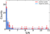 |
Fig. 1. Number of positive (red) and negative (i.e., noise; blue) peaks detected in the 118 ALPINE pointings as a function of the S/N. The errorbars are the Poissonian uncertanties. We can see that for S/N > 5.8 the number of positive peaks becomes higher than the number of the negative ones as the number of genuine detections with regard to spurious sources increases. |
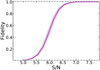 |
Fig. 2. Fidelity curve (purple solid line) for the serendipitous lines detected in ALPINE. The shaded area corresponds to the 1σ errorbars. The fidelity was computed by comparing the number of positive (genuine lines and noise peaks) and negative (only noise) peaks detected in the 118 ALPINE pointings. We see that the fidelity is a very steep function of the S/N. We adopted a fidelity threshold of 85% (corresponding to a S/N cutoff of 6.3) for the final catalog of the serendipitous lines. |
We used the fidelity to define the final catalog of the serendipitous lines. The fidelity threshold adopted at this step is crucial since the fraction of genuine detections in the final catalog depends on it. We included in it the lines with a fidelity higher than 85% (corresponding to a S/N = 6.30 cutoff), that is, there is a very low probability that they are spurious sources (see also the results of González-López et al. 2019; Decarli et al. 2020). This sample includes 12 robust line detections, with 10/12 sources with fidelity equal to unity. We added two more lines with lower fidelity (∼50%, corresponding to S/N ∼ 5.98) based on the fact that they present an optical/NIR counterpart2 (see Sect. 4). This provides a final catalog of 14 robust serendipitous line detections over the entire ALPINE pointings3. We note that the possibility that a (low) fraction of spurious sources with fidelity < 1 entering our sample does not constitute a problem in the computation of the [C II] LF, as each line is weighted by its fidelity value (see Sect. 5).
It is equally true that the adopted fidelity cut certainly excludes some genuine detections with low S/N from our catalog. Indeed, if we push the fidelity down to 20% (S/N = 5.69), we find ten more sources. According to their fidelity, we expect that the fraction of true sources is low (∼30%). However, their exclusion could have an impact on the derivation of the LF (see Sect. 5). We address this point in Sect. 5 and in Appendix B.
3.3. Completeness
Given the purpose of the present work, we need to also estimate the completeness of the sample, that is, the fraction of recovered lines with respect to the underlying population. We assessed the completeness by simulating ∼50 000 Gaussian-like lines with various peak flux F and FWHM and by injecting them in datacubes containing pure noise representative of the survey (0.14 Jy beam km s−1 over a line width of 235 km s−1). We injected the lines in random locations in the FOV and along the spectral axis, splitting them in groups of 15 lines per datacube in order to not artificially increase the source confusion. We simulated point sources (0.78″ × 1.16″) since the sources in our catalog are point-like or marginally resolved. However, we note that recent studies reported the existence of extended [C II] structures (e.g., Fujimoto et al. 2019, 2020; Ginolfi et al. 2020a,b), which may cause incompleteness for some faint objects (see Fig. 5 in Fujimoto et al. 2017). The simulated FWHM range is between 50 and 550 km s−1, while the peak flux varies between 1.0 mJy beam−1 and 12 mJy beam−1 in order to widely sample the parameter space of the detected lines (see Fig. 3). In particular, for each line the primary beam attenuation is taken into account, that is, its peak flux is lowered based on the primary beam response depending on its spatial position. We hence derived the completeness C in the jth cell of the (FWHM, F) grid as:
 (2)
(2)
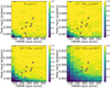 |
Fig. 3. Completeness (color scale) as a function of the flux peak and the FWHM of a line. The four diagrams correspond to the R< 30, R30−50, R50−70, and R70−90 regions respectively. As is evident from their comparison, the completeness is a strong function of the line location in the FOV because of the degrading sensitivity from the phase center to larger radii. The lines used to build the [C II] LF (see Sect. 5) are also shown (filled circles), except for the two brightes ones (i.e., S848185 and S842313), which are located outside the plotted ranges and have completeness equal to 1 everywhere in the FOV. We show the [C II] serendipitous detections in all the panels, independently from the line location in the FOV, since we computed their completeness in each ring when building the LF (see Eq. (3)). |
where  and
and  are the number of injected lines and recovered lines by findclumps in the cell. We considered cells of 50 km s−1 and 0.5 mJy beam−1 width. This cell size allows us to accurately evaluate the completeness, with an average number of 60 lines in each cell. We note that completeness is a strong function of the line location in the FOV since the sensitivity decreases significantly as the distance from the phase center increases. We thus evaluated it locally, splitting the lines in four regions based on the primary beam response. In particular, we defined four rings with radius R< 30, R30−50, R50−70, and R70−90, in which the primary beam attenuation goes from zero to a 30% (distance from the phase center R< 30 ≤ 7.1″), from 30% to 50% (7.1″ < R30−50 ≤ 10.4″), from 50% to 70% (10.4″ < R50−70 ≤ 13.1″), and from 70% to 90% (13.1″ < R70−90 ≤ 16.4″). We computed the completeness for each of these regions. We avoided the separation in narrower rings since it would have implied a poor statistics of fake sources to adequately sample the completeness.
The diagrams showing the completeness in the four rings are presented in Fig. 3. It seems clear from the plots that, for equal FWHM and peak flux, lines that are easily detected close to the phase center may become more difficult to detect when observed in the outskirts of the FOV. In addition, at a fixed flux peak, the completeness is higher for larger lines. We also show the location of the lines used to build the [C II] LF (see Sect. 5.1 and Table 1) in the parameter space (FWHM, F). All the lines have a completeness higher than 95% in the two most internal regions except for two cases that have completeness between 90% and 70%. In the remaining less sensitive rings the completeness is still higher than 65% in all the cases except for three sources with completeness values below 50%. This fact guarantees that we applied minimal completeness corrections to our lines when evaluating the LF (see Sect. 5).
Catalog of the serendipitous emitters in ALPINE (confirmed and candidates; the latter are marked with an *).
4. Identification and sources properties
In order to identify the detected lines, we cross–matched their spatial position with the entries in the COSMOS–2015 and 3D–HST photometric catalogs (Brammer et al. 2012; Laigle et al. 2016). The astrometry offsets between these catalogs and the ALMA maps are on the order of 0.1″ (Faisst et al. 2019). In addition, we checked for counterparts also in the SPLASH (Capak et al. 2012), UltraVista-DR4 (McCracken et al. 2012), 24 μm–selected (Le Floc’h et al. 2009) and 3 GHz-selected JVLA catalogs (Smolčić et al. 2017). Moreover, we also visually inspected the images from UV to mid–infrared (MIR) wavelegths in order to look for faint emissions not reported in the catalogs. We classified a galaxy as a physical counterpart of a serendipitous line if their spatial distance is less than 1″. The choice of this value derived from the distance distribution between the serendipitous lines and all the galaxies lying within 10″, which clearly presents a minimum for a distance ∼1″ for all the catalogs.
Based on the photometric or spectroscopic redshift available, we identified eight lines as [C II] and two lines as CO(Jup = 7, 5) transitions. The remaining four detections have an ambiguous identification because of the lack of an optical/NIR or uncertain photometric redshift from ancillary data4. All the images and spectra of the serendipitous lines are reported in Appendix A. We refer to a future paper for an analysis of the CO emitting galaxies (Loiacono et al., in prep.). Hereafter, we focus on the [C II] emitters and on the ambiguous lines (i.e., 12 objects in total).
4.1. [C II] serendipitous emitters at 4.3 < z < 5.4
We identified eight lines as [C II] based on the photometric or spectroscopic redshift of the optical/NIR counterpart available from ancillary data. Namely, four out of eight detections have an UV-optical spectroscopic redshift (M. Salvato, priv. comm.; Capak et al. 2008, 2011). The remaining four sources have photometric redshifts compatible with [C II] emission (Laigle et al. 2016). The sources have redshift of 4.3 < z < 5.4, which is as expected given the spectral coverage of ALPINE. We note that among the serendipitous [C II] emitters, we recovered the well-studied sub-mm galaxies of AzTEC–C17 (referred to here as S842313; Laigle et al. 2016; Schinnerer et al. 2008; Jones et al. 2017) and AzTEC–3 (S848185; Capak et al. 2011; Riechers et al. 2010, 2014).
In addition to these eight detections, we found four lines whose identification based on the available photometry is ambiguous. Two of them (S818760 and S859732) do not present any counterpart in the available catalogs or in the multiwavelength images (from UV to MIR). The lack of counterparts suggests that these emissions are produced from highly dusty and high-z sources or from gas-rich galaxies with low stellar masses. The most likely associations are thus [C II] at 4 < z < 6 or CO transitions at lower redshifts. However, S818760 is located within 3″ and has a velocity separation of < 300 km s−1 from the central target in the same pointing (see Fig. 4). As a consequence, it is very likely that it is produced by a companion or interacting source with the UV-target emitting [C II] but also proving to be optically faint (see also Jones et al. 2020). A similar argument applies to S51008226625. We note that the narrow FWHM of this line (∼50 km s−1, see Table 1 and Appendix A) could be suspicious and indicative of a spurious line, despite the high fidelity (89%) of the detection. However, this source has been detected in two independent ALPINE pointings targeting the same galaxy (i.e., vuds cosmos 5100822662 and DEIMOS COSMOS 514583, see Bethermin et al. 2020 for the details) so the notion that the spurious emission is due to a noise peak is very unlikely. Moreover, S5100822662 is detected in the multiwavelength photometric images (see Fig. 4), suggesting that the detection is indeed genuine. Based on the Laigle et al. (2016) catalog, it has a photometric redshift of 0.69. However, the strict association with the ALPINE target in the same pointing (Fig. 4) favors a high-z interpretation for this source with the ALMA emission likely due to the [C II] line. We also cannot rule out that the emission in the photometric images is produced by a foreground source that is not related to the ALMA detection (see also Pavesi et al. 2018). Finally, S665626 does not present any counterpart in any other band apart from K-band UltraVista image (Romano et al. 2020). This source was studied in detail by Romano et al. (2020) and their modeling seems to favor a [C II] interpretation rather than a CO line. Follow-up observations are needed to unambiguously confirm the nature of these four sources.
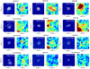 |
Fig. 4. Images cutouts of the 12 serendipitous lines used to build the [C II] LF. The HST-ACS 0.78 μm (Koekemoer et al. 2007, 2011) and Spitzer–IRAC 4.5 μm (Capak et al. 2012) are reported. The white contour shows the [C II] emission in steps of 2σ (lowest level at 3σ). We indicate with a white cross the location of the serendipitous detection while the red cross shows the position of the central target. We can see that for 6 out of 12 lines the distance between the central target and the serendipitous line is < 3″, hence, there is a possibility that we are witnessing interacting systems. For S5100822662, the [C II] emission is blended with that of the central target. |
In the rest of this work, we assume that the four unidentified lines are due to [C II] emission. We used both them and the confirmed [C II] to build the LF (Sect. 5). We note that the exclusion of the unidentified lines from it does not alter significantly any of the results. The optical/NIR images of the 12 serendipitous [C II] lines (confirmed and candidates) are shown in Fig. 4.
We estimated the main properties of the [C II] lines (i.e., frequency, FWHM, total fluxes) by performing a single-component Gaussian fit to the continuum subtracted spectrum, with the exception of source S842313, where two Gaussians were adopted to model the line profile (Appendix A) as it shows signs of rotation (Jones et al. 2017; see also Sect. 4.2 for further details about this source). To compute the line flux, we used the peak flux if the source size is comparable with the beam or we extracted it from a 3σ aperture in case the emission is resolved. To distinguish between resolved and unresolved sources, we compared the number of pixels within a 3σ aperture with the beam size in pixels. In case the number of pixels exceeds the beam size, we labeled the source as resolved. Otherwise, we considered the source as not resolved. Then we evaluated the deconvolved sizes of the resolved sources using the 2D fitting tool of CASA. We also measured the line fluxes on the moment zero maps, but we do not report them here since they show consistent results. All the fitted values are reported in Table 1.
4.2. Overdensities around the central targets
The detection of eight confirmed [C II] lines in targeted [C II] observations of 4 < z < 6 galaxies suggests that we are witnessing possible overdensities around the central UV-selected galaxies. This is highlighted by the velocity separation Δv between the central target and the serendipitous line in the same pointing. Indeed, seven out of eight [C II] lines have |Δv|< 750 km s−1, corresponding to a redshift separation |Δz|< 0.0154. Such a velocity difference suggests that the two galaxies in the same pointing could be physically connected or associated to the same large-scale structure. An extended protocluster at z ∼ 4.5 (PCI J1001+0220) in the COSMOS field was discovered by Lemaux et al. (2018). Capak et al. (2011) found another protocluster of galaxies in COSMOS at higher redshift (z ∼ 5.3; AzTEC–3 protocluster). In fact, some of the serendipitous lines in our sample (e.g., S848185) are well known members of these protoclusters. However, there are other detections in our catalog that could constitute potential new members of these protoclusters.
This is likely valid for two confirmed [C II] emitters (S5101209780, S5100969402) and one [C II] candidate (S665626) that lie in the spatial region corresponding to PCI J1001+0220 and have a redshift in the range 4.53 < z < 4.6 (Lemaux et al. 2018, 2020) while other three [C II] lines (two candidates and one confirmed) are possibly located in the outskirts of the same protocluster (Fig. 5; see also Ginolfi et al. 2020a). Further observations are necessary to confirm whether these three galaxies on the periphery are part of a greater structure associated with this protocluster. The same applies to the other sources in our sample (S787780, S873321, S378903, and S5100822662) that show a very low velocity separation with the UV-target in the same pointing but at the moment, it is unclear whether they are part of possible unknown protoclusters.
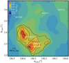 |
Fig. 5. Galaxy overdensity map of the PCI J1001+0220 protocluster at z ∼ 4.5 (Lemaux et al. 2018). The contour levels correspond to 2.5, 3.75, 5, 6.25, 7.5, 8.5σ. We see that three serendipitous sources (S665626, S5101209780, and S5100969402) are clearly associated to the protocluster, as their location is very close to two density peaks. On the other hand, S842313, S818760, and S859732 lie in the periphery of the overdense region of PCI J1001+0220. The spectroscopic data used to construct this map combines VUDS, zCOSMOS, and followup Keck/Deep Imaging Multi–Object Spectrograph (DEIMOS; Faber et al. 2003) observations. These spectroscopic data are used in conjunction with COSMOS–2015 photometric redshifts (Laigle et al. 2016) to generate the galaxy density map following Monte Carlo Voronoi tesselation technique (see Cucciati et al. 2018; Ginolfi et al. 2020a; Lemaux et al. 2020 for details on the method and data). |
Besides the low velocity and redshift separation, we also see that for four out of eight confirmed [C II] lines, the spatial separation from the central target is less then 3″, corresponding to a physical distance of < 20 kpc at z ∼ 5 (Fig. 4). The number of sources increases to six if we include also the [C II] candidates S818760 and S5100822662. These sources are galaxies that are likely interacting with the central targets. This is also suggested from the [C II] morphologies, which appear irregular as we can see for S5101209780 (Fig. 4). This source has been found to be part of a merging system of two massive galaxies (M⋆ ≳ 1010 M⊙) including two small satellites (Ginolfi et al. 2020a). Also large FWHM (> 500 km s−1) could be indicative of a merger. This scenario has been indeed suggested to explain the emission of S842313 (FWHM = 889 ± 35 km s−1; see Capak et al. 2008; Schinnerer et al. 2008). However, the regularity of the velocity field suggests that a disk interpretation is favored for this source (Jones et al. 2017).
Therefore, we could be in presence of two kind of overdensities: one on a very small scale (< 20 kpc) due to galaxy pairs or mergers and another on a larger scale (up to ∼90 kpc, i.e., the maximum distance allowed by the size of our pointings), related to possible more extended structures. We will analyze the overdense environment in more detail in a future paper (Loiacono et al., in prep.). The effect of clustering around the central UV targets has been taken into account when building the [C II] LF (see Sect. 5).
4.3. Relation between [C II] luminosity and SFR
Within the sample of the serendipitous [C II] lines, there are five sources for which also the continuum has been detected (Bethermin et al. 2020; Gruppioni et al. 2020). It is well known that there is a correlation between the [C II] luminosity and the SFR (De Looze et al. 2014). Since the latter is well-traced by the total IR luminosity (8−1000 μm), we used the five lines to test if this relation is also valid at z ∼ 5. We included also the two unconfirmed [C II] lines for which the ALMA continuum has been detected (S818760 and S665626).
The [C II] fluxes were converted to luminosities using Eq. (1) from Solomon et al. (1992) and we propagated the errors from the fitted quantities in Table 1. The total IR luminosity LIR was estimated from a SED fitting of the galaxies. We assumed the template of a star-forming galaxy that reproduces most of the Herschel galaxies at z ∼ 2−3 (Gruppioni et al. 2013). We note that the uncertainty on the total IR luminosity can be up to a factor of 5 depending on the assumed dust temperature (see Faisst et al. 2017; Fudamoto et al. 2020). This uncertainty accounts for about a factor ∼2.5 on the derived SFR, which we assumed as the typical error of this quantity. Then the LIR was converted to SFR using the Kennicutt (1998) relation.
If we compare our values with the local relation of De Looze et al. (2014, see their Table 3, case HII/starburst), we can see that they are broadly consistent within the 1σ errorbars (Fig. 6). On the other hand, our points suggest a slightly different slope compared to the model predictions at z = 5 of Lagache et al. (2018). The same trend is also shown by the ALPINE targets (Schaerer et al. 2020; Bethermin et al. 2020), which do not present any evidence of evolution of the SFR–L[C II] relation between z ∼ 0 and z ∼ 5. The only difference is that compared to the central UV-galaxies, the serendipitous sources reach higher SFRs and [C II] luminosities. In addition, we note that the SFR of the ALPINE targets takes into account both the UV and IR estimates; otherwise the UV–targets would not lie on the De Looze et al. (2014) relation (see Schaerer et al. 2020 for the details). On the other hand, we considered the IR-derived SFR only for the serendipitous galaxies. This means that the serendipitous sources detected both in line and continuum have SFRs dominated by the IR emission, with little or negligible contribution from the UV.
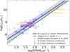 |
Fig. 6. SFR–L[C II] relation for the five serendipitous lines detected in continuum. The SFR of the serendipitous sources was computed from the IR luminosity. We can see that the sample is quite consistent at 1σ (colored area) with the De Looze et al. (2014) relation (purple line), suggesting that the contribution from the UV–traced SFR is negligible. We compare our results also with the models of Lagache et al. (2018) at z = 5 that suggest a slightly different slope. We also show the ALPINE UV–targets from Schaerer et al. (2020). Both the serendipitous sources and the ALPINE targets seems to suggest no evolution of the relation of De Looze et al. (2014). |
Therefore, both the ALPINE targets and the serendipitous sources appear to independently suggest that there is no significant variation of the relation of De Looze et al. (2014) up to z ∼ 5.
5. The [C II] luminosity function at z ∼ 5
5.1. Building the LF: “clustered” and “field” sources
The 14 [C II] lines (eight confirmed and four candidates) were used to build the LF. We populated each luminosity bin dlog L according to the relation:
 (3)
(3)
where Φ(L)d log L is the number density of [C II] emitters, Fj and  are the fidelity and completeness of the jth source associated to the comoving volume Vk. The latter was evaluated for the regions R< 30, R30−50, R50−70, and R70−90 in order to take into account the completeness variation in the FOV, hence the k index goes by the four rings. Only the sources with completeness and fidelity equal to unity everywhere in the FOV would have been indeed observable within the total comoving volume VTOT covered by the 118 ALPINE pointings. This volume was evaluated as
  Mpc3, where Ai is the area with a primary beam attenuation < 90% covered by each ALPINE pointing and ΔDc(zi) is the difference between the comoving distances of the [C II] line at the beginning and at the end of the ALMA sidebands for the ith pointing. This difference was computed after having excluded three to four channels at the beginning and at the end of each sideband to account for border effect (i.e., noisy channels). We note that we excluded the central R < 1″ region from each pointing in the computation of the volume. As the luminosity bin size, we considered 0.5 dex in order to have at least one source per bin. The adopted bin spacing is 0.25 dex in luminosity. Although the bins are not independent, this choice offers the advantage of better highlighting the luminosity distribution of the sample. We point out that we did not split the [C II] lines in different redshift bins because of the poor statistics, hence, our LF refers to an average redshift z ∼ 5. As done in Sect. 4.3, we evaluated the [C II] luminosities following Solomon et al. (1992) (see Table 1 for the values). The errorbars associated to each luminosity bin are computed as the Poissonian uncertainties corresponding to 1σ since the source number in each bin is small (Gehrels 1986), thus constituting the primary uncertainty.
Before computing the LF, we splitted the [C II] lines in two subsamples. As we see in Sect. 4, seven out of eight confirmed [C II] have a redshift separation from the central targets in the same pointings |Δz|< 0.015 (corresponding to a velocity separation < 750 km s−1). This number increases to 11 out of 12 if we include also the four unconfirmed [C II]. This means that their LF could be not representative of the field galaxy population since it is likely biased by the presence of overdensities around the UV-selected targets. The only exception is S510327576, which has a redshift separation of |Δz| = 0.2195 (|Δv|∼1.2 × 10⁴ km s−1) and is not, thus, related to the central target. This could be the only [C II] line not associated to clustered structures, that is, the only genuine field source in our sample.
In order to study the effect of clustering on the LF, we thus considered two separate subsamples, each of them containing the lines with a frequency offset from the central target lower or higher than one ALMA sideband (Δν ∼ 3.6 GHz; see Fig. 7). This separation corresponds to a redshift difference ≷0.04 and to a velocity separation ≷2000 km s−1 (see also Hennawi et al. 2010 who used a similar velocity separation in a study on quasars pairs). In this way we defined the “clustered” and “field” subsamples, containing 11 and 1 sources, respectively. Also the survey volume was split consistently, obatining a total comoving volume of 5026 Mpc3 for the clustered subsample and 4784 Mpc3 for the field one. Thus we built a separate [C II] LF for each sub–sample (Fig. 8 and Table 2). The median luminosity of the clustered sample (log(L/L⊙) = 8.96 ± 0.14) is very similar to the luminosity of the field one (log(L/L⊙) ∼ 9.0). However, we recall that the field LF is based on one object only and therefore it could also present galaxies at higher luminosity that we do not detect for the limited survey volume. Despite the similar median luminosity, the clustered LF shows objects with luminosity of about one order of magnitude higher than the field. If this trend were confirmed by a larger sample of galaxies, it would highlight a dependence between clustering and the [C II] luminosity, as has already been shown based with other tracers (e.g., Hawkins et al. 2001).
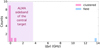 |
Fig. 7. Offset in frequency between the central UV target and the serendipitous [C II] in the same pointing. We see that the distribution is non-uniform, with several sources lying at a frequency (and hence a redshift) close to that of the central target. We thus defined two subsamples (named “clustered” and “field”, respectively) and evaluated two distinct LFs in order to account for any bias due to overdense regions. The separation between the two sample relies on the frequency width of one ALMA sideband (3.6 GHz), corresponding to a velocity separation ≷2000 km s−1. |
LFs for the clustered and field sample considering the eight confirmed and four candidates [C II].
In Appendix B, we report the LFs, including sources with a fidelity as low as 20% (see Fig. B.1). In Sect. 3.2, we cut indeed our catalog of serendipitous detections at a fidelity of 85%, with only one [C II] line (S5100969402) having a fidelity of ∼50% in order to study a very robust sample. However this sample is obviously incomplete at low luminosity. We thus calculated the clustered and field LFs for two new subsamples, in which we included also low fidelity (i.e., low luminosity) sources. The fidelity cut of 20% adds nine lines to our catalog of [C II] emitters (we excluded one single source that is possibly associated to CO emission; see Sect. 4). We note that none of these lines presents an optical/NIR counterpart, hence their redshift is unconstrained from ancillary data. Therefore, for these sources we can only assume that their emission is due to [C II]. We see that the shapes of both clustered and field LFs remain relatively unchanged, with the field LF sampled by more sources at this point. Also, in this case, the field sources lie at lower luminosities compared to the clustered sample. However, this is not surprising because as the fidelity is reduced, the line flux decreases and, hence, we expect the population of the low luminosity bins only for both field and clustered sources.
Finally, in Sect. 4.2 we show that the clustered sources are possibly part of two different types of overdensity – one associated to interactions and mergers (scale < 20 kpc) with the central UV-selected galaxy and the other associated to a more extended structure (up to ∼90 kpc). In order to overcome the bias introduced by the interacting systems, we excluded from the LF the six sources with a spatial distance of < 3″ from the central target (Fig. 4). We report the derived LF in Appendix B. The new points are consistent within the errors with the LF computed using all the clusterd sources. Overall, the faint end of the LF is lower compared to the case in which all the 11 clustered [C II] are considered. However, this has a negligible effect on the derivation of quantities, such as the fitted parameters of the Schechter function and the SFRD (see Sects. 5.3 and 6).
5.2. Comparison with observations and models
5.2.1. LFs from ALPINE
In this section, we discuss our LFs in relation to those from other works (Fig. 8). Overall, we consider the field LF as representative of the average population of galaxies while the clustered LF is likely biased to an high-density environment that is due to clustering around the central UV targets. The galaxies of the clustered sample are indeed companions of the ALPINE targets (see Sect. 5.1), which might not have been observed in a pure blind survey.
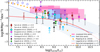 |
Fig. 8. [C II] LFs at z ∼ 5 from the serendipitous sources in ALPINE compared to other works in the literature. We split the lines in two subsamples, called “clustered” (pink) and “field” (azure), respectively, and we built two separate LFs. Compared to the clustered LF, the field one lies at lower luminosities. We compare our [C II] LFs at z ∼ 5 with other [C II] LFs at high and low-z. Overall, the estimates from the clustered sample lie above the LFs of the ALPINE targets (Yan et al. 2020) likely because they include UV-dark galaxies and because of the clustering effect. On the other hand, the field LF seems to be quite consistent with the targets ones except in the case of the highest luminosity bin. There is agreement between the field [C II] LF and the IR-derived [C II] LF based on the ALPINE serendipitous sources detected in continuum (Gruppioni et al. 2020). The agreement persists at L[C II] > 109.5 L⊙ for the clustered sample if the companions of the central targets are included in the IR-derived [C II] LF of Gruppioni et al. (2020). The clustered LF is up to > 1 dex higher than the local [C II] LF (Hemmati et al. 2017). Also the field LF predicts an excess of [C II] emitters at L[C II] > 109 L⊙, suggesting a possible evolution of the [C II] LF between z ∼ 5 and z ∼ 0. The field LF appears in agreement with the models predictions of Popping et al. (2019). |
We start by comparing our results with the other z ∼ 5 LFs based on the ALPINE data. First of all, we consider the [C II] LFs presented in the companion paper of Yan et al. (2020). These LFs were built using the 75 [C II] central UV targets in the two redshift ranges 4.40 < z < 4.58 and 5.13 < z < 5.85. Globally, we see that the clustered LF predicts more [C II] emitters than the Yan et al. (2020) sample. This was expected due to clustering effects and also because the LF of the central targets is based on UV-selected galaxies, hence it is likely to be missing the most obscured galaxies. On the other hand, the field LF is quite consistent with the targets LFs, showing a slight excess in the highest luminosity bin.
Thereafter, we compare our sample with the LF based on the sources serendipitously detected in the rest-frame FIR continuum (Gruppioni et al. 2020; Bethermin et al. 2020). The 118 ALPINE pointings have indeed revealed a wealth of serendipitous continuum emitters across a wide range of redshifts. These sources were used to build a LF at 250 μm (rest-frame) and a total IR LF from z = 0.5 to z = 6 (see Gruppioni et al. 2020 for details). For the purposes of our comparison, we considered the IR LF in the highest redshift interval 4.5 < z < 6, where the companions of the central targets have been removed (green water hexagons; see Table 4 of Gruppioni et al. 2020). The IR luminosities (8−1000 μm) were first converted to SFRs according to the Kennicutt (1998) relation. We note that the computed SFRs do not include the UV contribution, therefore, they can be considered as lower limits. However, we do not expect the UV contribution to be significant since the sources are selected to be dusty (i.e., FIR/sub-mm emitters). The SFRs were then used to derive the [C II] luminosities following the De Looze et al. (2014) relation (case of HII/starburst), scaled for a Chabrier (2003) IMF. Globally, the clustered LF presents a higher number density (up to about 1 dex) and higher luminosity objects than the IR-derived [C II] LF of Gruppioni et al. (2020). The difference in the lower luminosity bins is, however, enhanced by the fact that these bins are strongly incomplete in the continuum survey (see Bethermin et al. 2020). On the other hand, there is agreement between the field LF and the LF derived from Gruppioni et al. (2020). However, if we show the IR-derived [C II] LF that also includes the companions of the central targets for L[C II] > 109.5 L⊙ (magenta hexagons; see Gruppioni et al. 2020), we find that in this luminosity range the clustered [C II] LF and the IR-derived [C II] LF are nicely consistent within the errorbars. This is due to the fact that some of the sources included in these luminosity bins are the same, clustered around the central targets, detected both in line and in continuum.
5.2.2. Observed LFs at high and low-z
Now we can move on to comparing our results to other works in the literature, at both high and low-z. We see that our LFs are consistent with previous estimates at z = 4.4 and z ∼ 5 from Swinbank et al. (2012) and Capak et al. (2015). Swinbank et al. (2012) started from an original 870 μm selection of galaxies with LABOCA (Weiß et al. 2009) and considered the only two galaxies for which the [C II] line was detected in a subsequent ALMA follow-up. However, the low continuum detection rate of the ALPINE targets (20%; Bethermin et al. 2020) compared to the line detection rate (64%) suggests that a considerable fraction of [C II] emitting galaxies can be missed when starting from continuum pre-selected samples, hence the LF of Swinbank et al. (2012) likely provides a lower limit to the number density of the [C II] emitters. In case of the estimate from Capak et al. (2015), we use the value reported in Hemmati et al. (2017). Also, in this case, the data likely provide a lower limit to the true distribution, since the targets of Capak et al. (2015) are Lyman break galaxies, that is, UV-selected objects and, hence, [C II]-bright but optically-faint objects are not taken into account in this LF. Moreover, in this estimate the [C II] serendipitous emitters in the ten pointings of Capak et al. (2015) are not considered (e.g., AzTEC–3, Riechers et al. 2010; CRLE, Riechers et al. 2010).
Our values are consistent with the lower limit to the [C II] LF of Cooke et al. (2018). This study also provides a lower limit because it considers [C II] emitting galaxies pre-selected based on their SCUBA2 850 μm flux density (Geach et al. 2017).
We also compared our estimates with measurements at higher redshift (Yamaguchi et al. 2017). The points in Yamaguchi et al. (2017) represent upper limits to the [C II] LF at z ∼ 6. We can see that the field LF is consistent with the upper limits. On the other hand, the clustered LF seems to predict more [C II] emitters than Yamaguchi et al. (2017) at L[C II] = 108.75 L⊙ and that is probably because it is biased in favor of an overdense environment.
It is interesting to additionally compare our work with an extrapolation of the Herschel LF at z ∼ 5 (Gruppioni et al. 2013, and in prep.). The extrapolation was performed using the SCUBA2 number counts (Geach et al. 2017) to constrain the evolution at high redshift (Gruppioni & Pozzi 2019). The IR luminosities were thus converted to SFRs using the Kennicutt (1998) relation and the SFRs were transformed in [C II] luminosities following De Looze et al. (2014). We note that the same approach has been already used for deriving the CO LF in Vallini et al. (2016), which successfully reproduces the observed CO LF of ASPECS (Decarli et al. 2019). Interestingly, we see that the global shapes of the clustered LF and the Herschel–derived one are in good agreement, with both LFs predicting [C II] emitters with very high luminosities (L[C II] > 109 L⊙), with at least some of the discrepancy coming from the fact that the Herschel extrapolation was not intended to account for the clustering inherent in the ALPINE serendipitous sample.
Finally, we discuss how the z ∼ 5 [C II] LF compares with the z ∼ 0 values (Hemmati et al. 2017) to underline potential evolutionary effects. We can see that the clustered LF shows a strong evolution both in number density (up to > 1 dex) and in luminosity between z ∼ 0 and z ∼ 5. The field LF suggests also a possible excess of objects at L[C II] > 109 L⊙ compared to the local value. The two LFs are however consistent within 2σ. A higher statistics for the field sample is necessary to draw robust conclusions about any evolutionary trend that is independent from clustering.
5.2.3. Theoretical predictions
We also compare our results with model predictions for the early Universe. First of all, we considered the models for the [C II] LF by Popping et al. (2019). These are semi-analytical models that include radiative transfer modeling. We can see that the clustered [C II] LF predicts a higher number of objects than the models expectations at z ∼ 5, with a disagreement that rises with increasing luminosity. A similar disagreement with models predictions is seen also for the CO LFs at high-z (Riechers et al. 2019) and for the IR LF at z ∼ 2 (Gruppioni et al. 2015). On the other hand, the field LF appears quite consistent with the models. Further statistics would be useful to constrain the bright end of the field LF and disentangle if it remains flat at L[C II] > 109 L⊙ (as for the clustered sample) or if it declines as shown by models.
Then we examine the predictions at z ∼ 5 by Lagache et al. (2018). This is also a semi-analytic model combined with a photoionization code. We note that at luminosities between 109 L⊙ and 1010.5 L⊙ the Lagache et al. (2018) curve is not very different from the Herschel extrapolation. Compared to Popping et al. (2019), this model predicts more [C II] emitters at L[C II] > 109.5 L⊙, with luminosities consistent with the observed values for the clustered sample. However, we see that our observed LFs (especially the clustered one) show a higher number density of objects (> 1 dex), which is not predicted by this model.
5.3. Fitting with a Schechter function
We performed a fit to the [C II] LFs with the Schechter (1976) function written in logarithmic form (Fig. 9). Given the element of luminosity dlog L, the number of objects Φ(L)d log L falling in the bin is:
 (4)
(4)
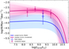 |
Fig. 9. Schechter functions for the clustered (pink) and field (azure) [C II] LFs. Also, the observed LFs corresponding to the independent luminosity bins are indicated (same color code). We fitted log Φ*, log L*, and α for the clustered LF using a Markov chain Monte Carlo (MCMC) method. We assumed for the field sample the same α and log L* of the clustered LF and we scaled the normalization of the clustered LF by a factor of 11 (corresponding to the ratio between the number of clustered and field sources). The shaded area (pink; clustered sample) shows the MCMC realizations within the 16th and 84th percentile, hence, it corresponds approximately to 1σ errorbars. In case of the scaled field LF, the 1σ errors (blue area) were computed from the uncertainties of log Φ* of the clustered sample and the Poissonian uncertainty (at 1σ) on 11 counts. |
where α is the faint-end slope and L* and Φ* are the luminosity and the value of the LF at the “knee”, respectively. For simplicity, we fitted the log Φ(L) and thus also the logarithms of L* and Φ*. We fitted the clustered LF only because of the low statistics of the field LF and the only one independent bin. Before perfoming the fit, we rebinned the clustered and field LF adopting a bin spacing of 0.5 dex instead of 0.25 dex (the bin width in Sect. 5.1). This ensures that the number counts in the bins are independent as well as the uncertainties on the fitted points.
To derive a first estimate of the fitted parameters, we performed a fit based on the maximum likelihood criterion. The best-fit values were used as initial guesses for a Markov chain Monte Carlo (MCMC) method with the Python package emcee (Foreman-Mackey et al. 2013). We assumed uniform priors for α, log L*, log Φ*. We preferred uniform priors over Gaussian ones as they represent the simplest possible choice since the probability distribution of these parameters is not known a priori. We note that the knee of the clustered LF is quite unconstrained by our data. This fact could clearly impact the derivation of the cosmic SFRD (see Sect. 6). In order to estimate log L*, we thus limited the upper boundary for the luminosity prior to 10.5, corresponding to an IR luminosity of 1013.5 L⊙ and assuming a fiducial ratio between [C II] and IR luminosity of 10−3 (Díaz-Santos et al. 2013). This is a reasonable upper boundary to the IR luminosity motivated by pre-existing IR LFs at lower redshifts (Gruppioni et al. 2013; Vallini et al. 2016). The validity of the L[C II]–SFR relation where the latter quantity is derived from continuum estimates for our sample (see Sect. 4.3) suggests that this is a trustworthy assumption.
The best values for α, log L*, log Φ* for the clustered LF are reported in Table 3. These values were evaluated as the medians of the posterior probability distributions. The reported uncertainties correspond to the 16th and 84th percentile of the posteriors (equivalent to about 1σ in the case of Gaussian posteriors).
Schechter parameters for the clustered and field LFs.
We then computed the Schechter function for the field LF as well. Since it was not possible to directly fit the data, we scaled Φ* by a factor 1/11 (i.e., the ratio between the number of field and clustered sources) based on the assumption that the shape of the two LFs is similar. In this way, the integration of the LF over the accessible volume and luminosity predicts a number of sources equal to the observed one (i.e., one source); see also Marshall et al. (1983). Moreover, this approach has the advantage of being independent of the binning of the LF. We obtained a value for  where the errors were propagated from the uncertainty on log Φ* of the clustered sample and the Poissonian error on the ratio 11:1. We note that the normalization determined in this way results consistent with the normalization that would be obtained by performing a Schechter fit to the field LF in which α and log L* are fixed to the clustered values. The Schechter functions of the clustered and field samples were used to estimate the cosmic SFRD (Sect. 6).
6. Star formation rate density at z ∼ 5
We know that the [C II] line is a SFR indicator (De Looze et al. 2014). Therefore the [C II] LF providing the total [C II] luminosity budget can be used to estimate the cosmic SFRD. First, we integrated the Schechter functions for the field and clustered sample in order to obtain the [C II] luminosity density ρL[C II] = ∫Φ(L′)L′d log L′. We considered in the integration all the luminosities higher than 107 L⊙. However, integrating from lower luminosities does not alter significantly the final estimates because the LFs are quite flat. In case of the clustered sample, the integration was performed for all the realizations of the MCMC. On the other hand, for the field sample, we integrated the best curve and the curves corresponding to the 1σ errorbars. Then we converted the luminosity densities to SFRDs using the relation (see Table 3 of De Looze et al. 2014; case HII/starburst)
![Mathematical equation: $$ \begin{aligned} \log {\dot{\rho }_{\star }} = - 7.06 + 1.00 \log {\rho _{L_{\rm [C\,II]}}} + \log {0.94}, \end{aligned} $$](/articles/aa/full_html/2021/02/aa38607-20/aa38607-20-eq24.gif) (5)
(5)
where  is the SFRD and the last term accounts for scaling the De Looze et al. (2014) relation from Kroupa (2001) to a Chabrier (2003) IMF. We note that the working assumption of a non-evolving L[C II]–SFR relation is not trivial (Vallini et al. 2015; Carniani et al. 2018). However, as we mention in Sect. 4.3, it seems to work at least for the serendipitous [C II] detected in continuum. Furthermore, the validity of this conversion is independently confirmed by the ALPINE targets which, as discussed in Bethermin et al. (2020) and Schaerer et al. (2020), lie within 1σ on the De Looze et al. (2014) relation. In this way, for the clustered sample we obtained a SFRD probability distribution based on all the MCMC realizations. We considered the median value of the distribution as the best estimate of the SFRD from the clustered sample and as done previously, we reported the uncertainties corresponding to the 16th and 84th percentile (Table 4). On the other hand, for the field sample, we considered the SFRD value corresponding to the integration of the best curve with the associated errorbars (see Fig. 9).
Cosmic SFRD from the clustered and field [C II] LFs.
In Fig. 10, we compare our results with previous estimates from the literature6 that are based on UV surveys (Schiminovich et al. 2005; Wyder et al. 2005; Dahlen et al. 2007; Reddy & Steidel 2009; Robotham & Driver 2011; Bouwens et al. 2012a,b, 2015; Cucciati et al. 2012; Schenker et al. 2013) as well as IR, mm, and radio selections of galaxies (Sanders et al. 2003; Takeuchi et al. 2003; Magnelli et al. 2011, 2013; Gruppioni et al. 2013; Rowan-Robinson et al. 2016; Dunlop et al. 2017; Novak et al. 2017). We also show the measurements derived from optical/NIR observations (Driver et al. 2018) and gamma-ray bursts (Kistler et al. 2009). We also plot the models predictions of Maniyar et al. (2018) based on the cosmic microwave background. Finally, we compare our results with other independent measurements of the SFRD based on the ALPINE data. In particular, we show the results derived from the serendipitous sources detected in continuum (Gruppioni et al. 2020) and the SFRD inferred from the ALPINE central targets (Khusanova et al. 2020).
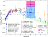 |
Fig. 10. Cosmic SFRD across cosmic time. Both the estimates from the “field” and “clustered” samples are shown (azure and pink box respectively). We compare our measurements with estimates available from the literature based on multiwavelength observations. The SFRD derived from the clustered [C II] LF at z ∼ 5 is about one order of magnitude higher than the current measurements at that redshift. On the other hand, the SFRD of the field sample spans values compatible with both UV and IR-derived estimates, with an average value a factor of ∼1.6 higher than the estimates based on UV surveys. We consider the SFRD from the field sample as representative of the overall galaxy population since the clustered estimate is biased by overdensities around the targeted [C II]. |
We can see that the SFRD derived from the clustered sample is almost 10× higher than the field value and the current estimates of the SFRD at z ∼ 5 from the literature. The high SFRD value predicted by the clustered sample could be indicative of the reversal of the SFR-density relation at high-z. This could be driven by the higher stellar mass content of clustered galaxies and by mechanisms due to the environment (Lemaux et al. 2020). However, we recall that only a fraction of the sources in the clustered sample are part of well-known overdensities (see Fig. 5 and Sect. 4.2), while the others are associated to galaxy pairs and mergers. A further investigation of the environment around these sources will be an important goal for future observations and facilities (e.g., JWST). We consider the SFRD computed using the field sample as the most likely estimate of the cosmic star formation activity at z ∼ 5. The measurement based on the clustered LF could indeed be biased by companions around the targeted [C II], which might not have been observed if we had started from a purely “blind” survey. Therefore, the clustered estimate may not be representative of the overall population of galaxies.
We do know that a relevant question deals with the relative contribution of the unobscured versus obscured star formation across cosmic time. The former is well-sampled by UV surveys from z ∼ 0 up to z ∼ 10 (Bouwens et al. 2015; Oesch et al. 2018). On the other hand, the latter is captured by surveys at longer wavelengths, typically IR and sub-mm. At the moment, the obscured star formation is well constrained by statistically robust samples up to z ∼ 3, whereas at higher redshift, its contribution to the total budget of star formation is quite uncertain. If we look at the average value of the SFRD based on the field LF, we can see that it is a factor of ∼1.6 higher than the measurement based on UV surveys (Bouwens et al. 2015). This means that it might be a fraction of (obscured) star formation that is not captured by UV surveys. However, when looking at the errors, we see that our estimate varies between values that are completely consistent with the UV estimates (i.e., neglible obscured star formation) to values that are about ten times higher than the UV measurements. A scenario consisting of a significant fraction of dust-obscured star formation already in place at z > 4 is suggested by IR, mm, and radio selections of galaxies (Bouwens et al. 2015; Novak et al. 2017; Gruppioni et al. 2020). Because of the large uncertainties, our measurement does not allow us to assess the importance of obscured versus unobscured star formation at z ∼ 5. Further observations of larger volumes of the sky are thus necessary to better constrain the [C II]-derived SFRD.
7. Summary and conclusions
In this work, we study the [C II] LF by using the lines serendipitously discovered in the ALMA ALPINE large program. This is the first LF at z ∼ 5 based on galaxies purely selected based on their [C II] line emission. We summarize the main results of this work:
-
First, we performed a blind search in the 118 ALPINE pointings, which revealed several unexpected lines. We assessed the fidelity and the completeness of the detections. The final catalog of the serendipitous sources includes 14 line emitters with high fidelity (> 85% for 12 out of 14 detections). We identified the line emission by comparing its spatial position with the available photometric catalogs and multiwavelength images. Out of the 14 lines, eight are [C II] lines at 4.3 < z < 5.4, supported by a spectroscopic or photometric redshift from ancillary data. Two out of 14 lines are CO transitions at lower redshift. Finally, four out of 14 lines exhibit a more tricky nature because they are not associated to any optical/NIR counterpart or they have an uncertain photometric redshift. However, three of them are very likely [C II] emitters based on the strict association with the central target or individual SED modeling. Observational follow-ups are necessary to allow us to unambiguously confirm the nature of these sources.
-
The eight [C II] emitters and the four lines with an ambiguos identification were used to build the [C II] LF. We found that 11 out of 12 sources are strongly clustered around the central target in the same poining since they are located at very similar redshifts (|Δz|< 0.0154, corresponding to |Δv|< 750 km s−1). The discovery of these sources could be very useful to investigate the properties of overdense regions at high-z and their study will be exhaustively addressed in a future work. In order to take the clustering into account when building the [C II] LF, we split our sample in two (i.e., “clustered” and “field” subsamples) based on the redshift separation between the serendipitous line and the central target in the same pointing and built two separate LFs. The median luminosity of the field and clustered samples is very similar; however, the clustered LF includes objects with luminosities that are a factor of ∼10 higher than the luminosity of the one galaxy in the field sample. If this trend were confirmed by a larger sample of galaxies, it could highlight the already known dependence between clustering and luminosity, which is witnessed for the first time from the [C II] line at z ∼ 5.
-
We compared our LFs with other works, both observational and theoretical. We found that, globally, the clustered LF suggests an excess of sources compared to the LFs of the ALPINE targets (Yan et al. 2020). This is not surprising since the clustered LF is likely biased to an overdense environment around the UV targets that is not representative of the average population of galaxies. Moreover, this discrepancy could be due to the fact that the targets LFs are based on UV-selected galaxies, hence, they do not include highly dusty objects. The clustered LF shows also an excess when compared to models predictions (Lagache et al. 2018; Popping et al. 2019) probably due to clustering. On the other hand, the field LF is quite consistent with the targets LFs. Our measurements, especially the field one, are quite in agreement with the estimates from the serendipitous continuum sources found in ALPINE (Gruppioni et al. 2020). The estimates from the field LF are also in agreement with the semi-analytical models of Popping et al. (2019) at L[C II] ∼ 109 L⊙. Observations of more extended volumes will be useful to assess whether this agreement persists also at higher luminosities. Finally, both the clustered and field LFs suggest a possible evolution of the [C II] LF from z ∼ 5 to z ∼ 0. Also, in this case, observations of larger samples are necessary to confirm this trend.
-
We performed a Schechter fit to the clustered LF. Then we scaled the fitted normalization function for a factor of 11 (corresponding to the ratio between the number of clustered and field sources) to reproduce the field LF under the assumption that they have the same shape. From the Schechter fits, we estimated the [C II] luminosity density. This value was then converted to the SFRD using the relation of De Looze et al. (2014) for the case of HII/starburst. We found that the clustered sample shows values that are up to a factor of ∼10 higher than the current estimates from the literature. This high SFRD value could be a hint of the reversal of the SFR-density relation (Lemaux et al. 2020). Further observations of the environment around the ALPINE targets will be useful in confirming this aspect. We considered the estimate obtained for the field sample as representative of the average galaxy population since the clustered estimate could be biased towards a high-density environment. The average SFRD is a factor of ∼1.6, on average, higher than the current estimates from UV surveys. However, because of the large errorbars, it is not possible for us to determine whether this value could be indicative of a significant fraction of obscured star formation at z ∼ 5, as has been suggested by IR and mm selections of galaxies. Observations of larger samples are necessary to better constrain the SFRD of the Universe.
This work represents the first effort to study the luminosity function of [C II] emitters at z ∼ 5 with sources strictly selected based on their [C II] emission. It provides new insights into the properties of the star-forming medium in a poorly known cosmic epoch.
We note that this survey area is higher than the area reported by Bethermin et al. (2020) since we included in our estimate a region where the primary beam attenuation reaches the 90%, while in Bethermin et al. (2020), the 80% region has been considered.
We note that in addition to present a counterpart, one of the sources with fidelity ∼50% (i.e., S460378, see Table 1) has been detected also in continuum with high significance (Bethermin et al. 2020), so despite its low fidelity, it is likely to be associated to genuine emission.
We note that among the detections in the final catalog, there is one source (S848185, see Table 1) that is located at the periphery of the primary beam, i.e., in a region with very poor sensitivity (≲20%). Despite this, the high S/N (∼16) of the detection makes it one of the most reliable sources in our sample.
We note that if we consider the sources with a fidelity down to 20%, nine out of the ten new sources do not show any optical/NIR counterpart. There is only one detection associated to a galaxy with a photometric redshift that makes the line emission compatible with a CO(4–3), CO(5–4) or [C I] transition.
We note that this particular source was included also in the LF of Yan et al. (2020), as they used the total flux of the central target vuds cosmos 5100822662 (see also Fig. 4), which was not deblended from the serendipitous companion (see Bethermin et al. 2020). However, since the latter respects the criterion to be a non-target source (i.e., distance from the phase higher than 1″), we included it in our calculations. We note that its exclusion from our sample does not alter the result significantly.
For works prior to 2014, we show the values reported in Table 1 of Madau & Dickinson (2014), except for Kistler et al. (2009), which is not included in the table.
Acknowledgments
This paper is dedicated to the memory of Olivier Le Févre, PI of the ALPINE survey. This paper is based on data obtained with the ALMA Observatory, under Large Program 2017.1.00428.L. ALMA is a partnership of ESO (representing its member states), NSF (USA) and NINS (Japan), together with NRC (Canada), MOST and ASIAA (Taiwan), and KASI (Republic of Korea), in cooperation with the Republic of Chile. The Joint ALMA Observatory is operated by ESO, AUI/NRAO and NAOJ. Based on data products from observations made with ESO Telescopes at the La Silla Paranal Observatory under ESO programme ID 179.A-2005 and on data products produced by TERAPIX and the Cambridge Astronomy Survey Unit on behalf of the UltraVISTA consortium. This program is supported by the national program Cosmology and Galaxies from the CNRS in France. Some of the material presented in this paper is based upon work supported by the National Science Foundation under Grant No. 1908422. Some of the spectrographic data presented herein were obtained at the W.M. Keck Observatory, which is operated as a scientific partnership among the California Institute of Technology, the University of California, and the National Aeronautics and Space Administration. The Observatory was made possible by the generous financial support of the W.M. Keck Foundation. We thank the indigenous Hawaiian community for allowing us to be guests on their sacred mountain, a privilege without which this work would not have been possible. We are most fortunate to be able to conduct observations from this site. F.L., C.G., A.C., F.P., and M.T. acknowledge the support from the grant PRIN MIUR 2017. D.R. acknowledges support from the National Science Foundation under grant numbers AST-1614213 and AST-1910107 and from the Alexander von Humboldt Foundation through a Humboldt Research Fellowship for Experienced Researchers. G.C.J. acknowledges ERC Advanced Grant 695671 “QUENCH” and support by the Science and Technology Facilities Council (STFC). GL acknowledges support from the European Research Council (ERC) under the European Union’s Horizon 2020 research and innovation programme (project CONCERTO, grant agreement No 788212) and from the Excellence Initiative of Aix-Marseille University-A*Midex, a French “Investissements d’Avenir” programme.
References
- Aravena, M., Decarli, R., Gónzalez-López, J., et al. 2019, ApJ, 882, 136 [CrossRef] [Google Scholar]
- Ashby, M. L. N., Willner, S. P., Fazio, G. G., et al. 2013, ApJ, 769, 80 [NASA ADS] [CrossRef] [Google Scholar]
- Bethermin, M., Fudamoto, Y., Ginolfi, M., et al. 2020, A&A, 643, A2 [CrossRef] [EDP Sciences] [Google Scholar]
- Bouwens, R. J., Illingworth, G. D., Oesch, P. A., et al. 2012a, ApJ, 754, 83 [NASA ADS] [CrossRef] [Google Scholar]
- Bouwens, R. J., Illingworth, G. D., Oesch, P. A., et al. 2012b, ApJ, 752, L5 [NASA ADS] [CrossRef] [Google Scholar]
- Bouwens, R. J., Illingworth, G. D., Oesch, P. A., et al. 2015, ApJ, 803, 34 [Google Scholar]
- Bouwens, R. J., Aravena, M., Decarli, R., et al. 2016, ApJ, 833, 72 [NASA ADS] [CrossRef] [Google Scholar]
- Bowler, R. A. A., Jarvis, M. J., Dunlop, J. S., et al. 2020, MNRAS, 493, 2059 [CrossRef] [Google Scholar]
- Brammer, G. B., van Dokkum, P. G., Franx, M., et al. 2012, ApJS, 200, 13 [Google Scholar]
- Capak, P., Carilli, C. L., Lee, N., et al. 2008, ApJ, 681, L53 [Google Scholar]
- Capak, P. L., Riechers, D., Scoville, N. Z., et al. 2011, Nature, 470, 233 [Google Scholar]
- Capak, P., Aussel, H., Bundy, K., et al. 2012, SPLASH: Spitzer Large Area Survey with Hyper-Suprime-Cam, (Spitzer Proposal) [Google Scholar]
- Capak, P. L., Carilli, C., Jones, G., et al. 2015, Nature, 522, 455 [NASA ADS] [CrossRef] [Google Scholar]
- Cardamone, C. N., van Dokkum, P. G., Urry, C. M., et al. 2010, ApJS, 189, 270 [NASA ADS] [CrossRef] [Google Scholar]
- Carniani, S., Maiolino, R., Amorin, R., et al. 2018, MNRAS, 478, 1170 [NASA ADS] [CrossRef] [Google Scholar]
- Chabrier, G. 2003, PASP, 115, 763 [Google Scholar]
- Cooke, E. A., Smail, I., Swinbank, A. M., et al. 2018, ApJ, 861, 100 [Google Scholar]
- Cormier, D., Lebouteiller, V., Madden, S. C., et al. 2012, A&A, 548, A20 [NASA ADS] [CrossRef] [EDP Sciences] [Google Scholar]
- Cucciati, O., Tresse, L., Ilbert, O., et al. 2012, A&A, 539, A31 [NASA ADS] [CrossRef] [EDP Sciences] [Google Scholar]
- Cucciati, O., Lemaux, B. C., Zamorani, G., et al. 2018, A&A, 619, A49 [NASA ADS] [CrossRef] [EDP Sciences] [Google Scholar]
- Daddi, E., Dannerbauer, H., Liu, D., et al. 2015, A&A, 577, A46 [NASA ADS] [CrossRef] [EDP Sciences] [Google Scholar]
- Dahlen, T., Mobasher, B., Dickinson, M., et al. 2007, ApJ, 654, 172 [NASA ADS] [CrossRef] [Google Scholar]
- De Looze, I., Cormier, D., Lebouteiller, V., et al. 2014, A&A, 568, A62 [NASA ADS] [CrossRef] [EDP Sciences] [Google Scholar]
- Decarli, R., Walter, F., Aravena, M., et al. 2016, ApJ, 833, 69 [Google Scholar]
- Decarli, R., Walter, F., Gónzalez-López, J., et al. 2019, ApJ, 882, 138 [Google Scholar]
- Decarli, R., Aravena, M., Boogaard, L., et al. 2020, ApJ, 902, 110 [Google Scholar]
- Díaz-Santos, T., Armus, L., Charmandaris, V., et al. 2013, ApJ, 774, 68 [NASA ADS] [CrossRef] [Google Scholar]
- Dickinson, M., Giavalisco, M., & GOODS Team 2003, in The Mass of Galaxies at Low and High Redshift, eds. R. Bender, & A. Renzini, 324 [CrossRef] [Google Scholar]
- Driver, S. P., Andrews, S. K., da Cunha, E., et al. 2018, MNRAS, 475, 2891 [NASA ADS] [CrossRef] [Google Scholar]
- Dunlop, J. S., McLure, R. J., Biggs, A. D., et al. 2017, MNRAS, 466, 861 [Google Scholar]
- Elbaz, D., Dickinson, M., Hwang, H. S., et al. 2011, A&A, 533, A119 [NASA ADS] [CrossRef] [EDP Sciences] [Google Scholar]
- Faber, S. M., Phillips, A. C., Kibrick, R. I., et al. 2003, in Instrument Design and Performance for Optical/Infrared Ground-based Telescopes, eds. M. Iye, & A. F. M. Moorwood, SPIE Conf. Ser., 4841, 1657 [Google Scholar]
- Faisst, A. L., Capak, P. L., Yan, L., et al. 2017, ApJ, 847, 21 [NASA ADS] [CrossRef] [Google Scholar]
- Faisst, A. L., Schaerer, D., Lemaux, B. C., et al. 2019, ApJS, 247, 61 [CrossRef] [Google Scholar]
- Finkelstein, S. L. 2016, PASA, 33, e037 [NASA ADS] [CrossRef] [Google Scholar]
- Foreman-Mackey, D., Hogg, D. W., Lang, D., & Goodman, J. 2013, PASP, 125, 306 [Google Scholar]
- Fudamoto, Y., Oesch, P. A., Faisst, A., et al. 2020, A&A, 643, A4 [CrossRef] [EDP Sciences] [Google Scholar]
- Fujimoto, S., Ouchi, M., Shibuya, T., & Nagai, H. 2017, ApJ, 850, 83 [NASA ADS] [CrossRef] [Google Scholar]
- Fujimoto, S., Ouchi, M., Ferrara, A., et al. 2019, ApJ, 887, 107 [NASA ADS] [CrossRef] [Google Scholar]
- Fujimoto, S., Silverman, J. D., Bethermin, M., et al. 2020, ApJ, 900, 1 [CrossRef] [Google Scholar]
- Geach, J. E., Dunlop, J. S., Halpern, M., et al. 2017, MNRAS, 465, 1789 [Google Scholar]
- Gehrels, N. 1986, ApJ, 303, 336 [NASA ADS] [CrossRef] [Google Scholar]
- Giavalisco, M., Ferguson, H. C., Koekemoer, A. M., et al. 2004, ApJ, 600, L93 [NASA ADS] [CrossRef] [Google Scholar]
- Ginolfi, M., Jones, G. C., Bethermin, M., et al. 2020a, A&A, 643, A7 [CrossRef] [EDP Sciences] [Google Scholar]
- Ginolfi, M., Jones, G. C., Béthermin, M., et al. 2020b, A&A, 633, A90 [CrossRef] [EDP Sciences] [Google Scholar]
- González-López, J., Decarli, R., Pavesi, R., et al. 2019, ApJ, 882, 139 [CrossRef] [Google Scholar]
- Gruppioni, C., & Pozzi, F. 2019, MNRAS, 483, 1993 [NASA ADS] [CrossRef] [Google Scholar]
- Gruppioni, C., Pozzi, F., Rodighiero, G., et al. 2013, MNRAS, 432, 23 [NASA ADS] [CrossRef] [Google Scholar]
- Gruppioni, C., Calura, F., Pozzi, F., et al. 2015, MNRAS, 451, 3419 [NASA ADS] [CrossRef] [Google Scholar]
- Gruppioni, C., Bethermin, M., Loiacono, F., et al. 2020, A&A, 643, A8 [CrossRef] [EDP Sciences] [Google Scholar]
- Guo, Y., Ferguson, H. C., Giavalisco, M., et al. 2013, ApJS, 207, 24 [NASA ADS] [CrossRef] [Google Scholar]
- Hawkins, E., Maddox, S., Branchini, E., & Saunders, W. 2001, MNRAS, 325, 589 [NASA ADS] [CrossRef] [Google Scholar]
- Hemmati, S., Yan, L., Diaz-Santos, T., et al. 2017, ApJ, 834, 36 [NASA ADS] [CrossRef] [Google Scholar]
- Hennawi, J. F., Myers, A. D., Shen, Y., et al. 2010, ApJ, 719, 1672 [NASA ADS] [CrossRef] [Google Scholar]
- Hollenbach, D. J., & Tielens, A. G. G. M. 1999, Rev. Mod. Phys., 71, 173 [Google Scholar]
- Jones, G. C., Carilli, C. L., Shao, Y., et al. 2017, ApJ, 850, 180 [NASA ADS] [CrossRef] [Google Scholar]
- Jones, G. C., Béthermin, M., Fudamoto, Y., et al. 2020, MNRAS, 491, L18 [Google Scholar]
- Karim, A., Swinbank, A. M., Hodge, J. A., et al. 2013, MNRAS, 432, 2 [NASA ADS] [CrossRef] [Google Scholar]
- Kennicutt, R. C., Jr. 1998, ApJ, 498, 541 [NASA ADS] [CrossRef] [Google Scholar]
- Khusanova, Y., Béthermin, M., Le Fèvre, O., et al. 2020, A&A, submitted [arXiv:2007.08384] [Google Scholar]
- Kistler, M. D., Yüksel, H., Beacom, J. F., Hopkins, A. M., & Wyithe, J. S. B. 2009, ApJ, 705, L104 [NASA ADS] [CrossRef] [Google Scholar]
- Koekemoer, A. M., Aussel, H., Calzetti, D., et al. 2007, ApJS, 172, 196 [NASA ADS] [CrossRef] [Google Scholar]
- Koekemoer, A. M., Faber, S. M., Ferguson, H. C., et al. 2011, ApJS, 197, 36 [NASA ADS] [CrossRef] [Google Scholar]
- Kohandel, M., Pallottini, A., Ferrara, A., et al. 2019, MNRAS, 487, 3007 [NASA ADS] [CrossRef] [Google Scholar]
- Kroupa, P. 2001, MNRAS, 322, 231 [NASA ADS] [CrossRef] [Google Scholar]
- Lagache, G., Cousin, M., & Chatzikos, M. 2018, A&A, 609, A130 [NASA ADS] [CrossRef] [EDP Sciences] [Google Scholar]
- Laigle, C., McCracken, H. J., Ilbert, O., et al. 2016, ApJS, 224, 24 [NASA ADS] [CrossRef] [Google Scholar]
- Le Fèvre, O., Béthermin, M., Faisst, A., et al. 2020, A&A, 643, A1 [CrossRef] [EDP Sciences] [Google Scholar]
- Le Floc’h, E., Aussel, H., Ilbert, O., et al. 2009, ApJ, 703, 222 [NASA ADS] [CrossRef] [Google Scholar]
- Lemaux, B. C., Le Fèvre, O., Cucciati, O., et al. 2018, A&A, 615, A77 [NASA ADS] [CrossRef] [EDP Sciences] [Google Scholar]
- Lemaux, B. C., Cucciati, O., Le Fèvre, O., et al. 2020, A&A, submitted [arXiv:2009.03324] [Google Scholar]
- Liu, D., Schinnerer, E., Groves, B., et al. 2019, ApJ, 887, 235 [Google Scholar]
- Lutz, D., Poglitsch, A., Altieri, B., et al. 2011, A&A, 532, A90 [NASA ADS] [CrossRef] [EDP Sciences] [Google Scholar]
- Madau, P., & Dickinson, M. 2014, ARA&A, 52, 415 [NASA ADS] [CrossRef] [Google Scholar]
- Magdis, G. E., Rigopoulou, D., Hopwood, R., et al. 2014, ApJ, 796, 63 [Google Scholar]
- Magnelli, B., Elbaz, D., Chary, R. R., et al. 2011, A&A, 528, A35 [NASA ADS] [CrossRef] [EDP Sciences] [Google Scholar]
- Magnelli, B., Popesso, P., Berta, S., et al. 2013, A&A, 553, A132 [NASA ADS] [CrossRef] [EDP Sciences] [Google Scholar]
- Maniyar, A. S., Béthermin, M., & Lagache, G. 2018, A&A, 614, A39 [NASA ADS] [CrossRef] [EDP Sciences] [Google Scholar]
- Marchesi, S., Civano, F., Elvis, M., et al. 2016, ApJ, 817, 34 [Google Scholar]
- Marshall, H. L., Tananbaum, H., Zamorani, G., et al. 1983, ApJ, 269, 42 [Google Scholar]
- Matthee, J., Sobral, D., Boogaard, L. A., et al. 2019, ApJ, 881, 124 [NASA ADS] [CrossRef] [Google Scholar]
- McCracken, H. J., Milvang-Jensen, B., Dunlop, J., et al. 2012, A&A, 544, A156 [NASA ADS] [CrossRef] [EDP Sciences] [Google Scholar]
- Novak, M., Smolčić, V., Delhaize, J., et al. 2017, A&A, 602, A5 [NASA ADS] [CrossRef] [EDP Sciences] [Google Scholar]
- Novak, M., Bañados, E., Decarli, R., et al. 2019, ApJ, 881, 63 [NASA ADS] [CrossRef] [Google Scholar]
- Oesch, P. A., Bouwens, R. J., Illingworth, G. D., Labbé, I., & Stefanon, M. 2018, ApJ, 855, 105 [NASA ADS] [CrossRef] [Google Scholar]
- Pallottini, A., Ferrara, A., Decataldo, D., et al. 2019, MNRAS, 487, 1689 [NASA ADS] [CrossRef] [Google Scholar]
- Pavesi, R., Riechers, D. A., Capak, P. L., et al. 2016, ApJ, 832, 151 [NASA ADS] [CrossRef] [Google Scholar]
- Pavesi, R., Riechers, D. A., Sharon, C. E., et al. 2018, ApJ, 861, 43 [NASA ADS] [CrossRef] [Google Scholar]
- Popping, G., Narayanan, D., Somerville, R. S., Faisst, A. L., & Krumholz, M. R. 2019, MNRAS, 482, 4906 [Google Scholar]
- Reddy, N. A., & Steidel, C. C. 2009, ApJ, 692, 778 [NASA ADS] [CrossRef] [Google Scholar]
- Riechers, D. A., Capak, P. L., Carilli, C. L., et al. 2010, ApJ, 720, L131 [NASA ADS] [CrossRef] [Google Scholar]
- Riechers, D. A., Bradford, C. M., Clements, D. L., et al. 2013, Nature, 496, 329 [Google Scholar]
- Riechers, D. A., Carilli, C. L., Capak, P. L., et al. 2014, ApJ, 796, 84 [NASA ADS] [CrossRef] [Google Scholar]
- Riechers, D. A., Pavesi, R., Sharon, C. E., et al. 2019, ApJ, 872, 7 [Google Scholar]
- Robotham, A. S. G., & Driver, S. P. 2011, MNRAS, 413, 2570 [Google Scholar]
- Rodighiero, G., Daddi, E., Baronchelli, I., et al. 2011, ApJ, 739, L40 [NASA ADS] [CrossRef] [Google Scholar]
- Romano, M., Cassata, P., Morselli, L., et al. 2020, MNRAS, 496, 875 [CrossRef] [Google Scholar]
- Rowan-Robinson, M., Oliver, S., Wang, L., et al. 2016, MNRAS, 461, 1100 [NASA ADS] [CrossRef] [Google Scholar]
- Sanders, D. B., Mazzarella, J. M., Kim, D. C., Surace, J. A., & Soifer, B. T. 2003, AJ, 126, 1607 [Google Scholar]
- Sanders, D. B., Salvato, M., Aussel, H., et al. 2007, ApJS, 172, 86 [Google Scholar]
- Schaerer, D., Ginolfi, M., Bethermin, M., et al. 2020, A&A, 643, A3 [CrossRef] [EDP Sciences] [Google Scholar]
- Schechter, P. 1976, ApJ, 203, 297 [Google Scholar]
- Schenker, M. A., Robertson, B. E., Ellis, R. S., et al. 2013, ApJ, 768, 196 [NASA ADS] [CrossRef] [Google Scholar]
- Schiminovich, D., Ilbert, O., Arnouts, S., et al. 2005, ApJ, 619, L47 [NASA ADS] [CrossRef] [Google Scholar]
- Schinnerer, E., Carilli, C. L., Capak, P., et al. 2008, ApJ, 689, L5 [Google Scholar]
- Scoville, N., Aussel, H., Brusa, M., et al. 2007, ApJS, 172, 1 [NASA ADS] [CrossRef] [Google Scholar]
- Scoville, N., Lee, N., Vanden Bout, P., et al. 2017, ApJ, 837, 150 [NASA ADS] [CrossRef] [Google Scholar]
- Smit, R., Bouwens, R. J., Carniani, S., et al. 2018, Nature, 553, 178 [NASA ADS] [CrossRef] [Google Scholar]
- Smolčić, V., Novak, M., Bondi, M., et al. 2017, A&A, 602, A1 [NASA ADS] [CrossRef] [EDP Sciences] [Google Scholar]
- Solomon, P. M., Downes, D., & Radford, S. J. E. 1992, ApJ, 398, L29 [NASA ADS] [CrossRef] [Google Scholar]
- Speagle, J. S., Steinhardt, C. L., Capak, P. L., & Silverman, J. D. 2014, ApJS, 214, 15 [NASA ADS] [CrossRef] [Google Scholar]
- Swinbank, A. M., Karim, A., Smail, I., et al. 2012, MNRAS, 427, 1066 [Google Scholar]
- Tacconi, L. J., Genzel, R., Saintonge, A., et al. 2018, ApJ, 853, 179 [NASA ADS] [CrossRef] [Google Scholar]
- Takeuchi, T. T., Yoshikawa, K., & Ishii, T. T. 2003, ApJ, 587, L89 [NASA ADS] [CrossRef] [Google Scholar]
- Vallini, L., Gallerani, S., Ferrara, A., Pallottini, A., & Yue, B. 2015, ApJ, 813, 36 [NASA ADS] [CrossRef] [Google Scholar]
- Vallini, L., Gruppioni, C., Pozzi, F., Vignali, C., & Zamorani, G. 2016, MNRAS, 456, L40 [Google Scholar]
- Walter, F., Decarli, R., Carilli, C., et al. 2012, Nature, 486, 233 [Google Scholar]
- Walter, F., Decarli, R., Aravena, M., et al. 2016, ApJ, 833, 67 [Google Scholar]
- Weiß, A., Kovács, A., Coppin, K., et al. 2009, ApJ, 707, 1201 [NASA ADS] [CrossRef] [Google Scholar]
- Wolfire, M. G., McKee, C. F., Hollenbach, D., & Tielens, A. G. G. M. 2003, ApJ, 587, 278 [NASA ADS] [CrossRef] [Google Scholar]
- Wyder, T. K., Treyer, M. A., Milliard, B., et al. 2005, ApJ, 619, L15 [Google Scholar]
- Yamaguchi, Y., Kohno, K., Tamura, Y., et al. 2017, ApJ, 845, 108 [NASA ADS] [CrossRef] [Google Scholar]
- Yan, L., Sajina, A., Loiacono, F., et al. 2020, ApJ, 905, 147 [Google Scholar]
Appendix A: Images and spectra
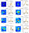 |
Fig. A.1. Continumm-subtracted ALMA maps and spectra of the 14 serendipitous lines found in the 118 ALPINE pointings. Each panel is labeled according to the number of the ALPINE source in the same pointing. We report the contours in steps of 2σ. The lowest level corresponds to 3σ. We fitted the line emission (black) using a sigle Gaussian component (orange). In the case of S842313, we fitted the line profile using two Gaussian components (cyan and red); the total model is shown in orange. For S5100822662, the serendipitous source is the small blob above the ALPINE target. The blob is marked with a cross and we present a spectrum extracted from its peak spaxel. |
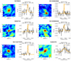 |
Fig. A.1. continued. |
Appendix B: Luminosity function
In this section, we show the [C II] LF computed including sources with a fidelity of > 20% (Fig. B.1 and Table B.1). In Sect. 3.2 we included in our catalog only the detections with fidelity > 85%, with only one [C II] emitter (S5100969402) having a fidelity of ∼50%, in order to study a very robust sample. However, this sample is obviously incomplete at the lowest luminosities. We thus derived the clustered and field LFs for two new subsamples, in which we included also low fidelity (i.e., low luminosity) sources. The fidelity cut of 20% adds 10 lines to our catalog of serendipitous detections. Based on their individual fidelities, we expect that only ∼3 out of the 10 lines are genuine detections, thus, this new sample is expected to contain a high fraction of spurious sources. One line is possibly associated to CO emission at z < 5 (see Sect. 4). The remaining nine do not present any optical/NIR counterpart, hence their redshift is unconstrained from ancillary data. Therefore, for these sources we can only assume that their emission is due to the [C II] line. We see that the shape of both clustered/field LFs remains quite unchanged, with the field LF sampled by more sources now. The field sources lie at lower luminosities compared to the clustered sample. However, this is not surprising given that as the fidelity is reduced, the line flux also decreases and, hence, we expect to obtain the population of the low-luminosity bins only for both field and clustered sources. We show also the [C II] LF (clustered sample) we obtained, excluding the six [C II] lines that are possibly associated to mergers or interactions (Fig. B.2 and Table B.2). The new points are consistent within the errors with respect to the old ones.
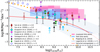 |
Fig. B.1. [C II] LFs at z ∼ 5 of the serendipitous sources in ALPINE including the sources with low fidelity. Compared to the clustered LF, the field one lies at lower luminosity. Both LFs result compatible with those based on the sources with higher fidelity. The main difference is at the low luminosity end since more sources are included in this sample. |
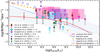 |
Fig. B.2. [C II] LF at z ∼ 5 of the clustered sources after removing the six [C II]–emitters associated to interacting galaxies with the central targets (see Fig. 4). Compared to the LF presented in Sect. 5, this one results in lower values at the faint end. |
LFs for the clustered and field sample considering the 21 sources with fidelity higher than 20%.
LFs for the clustered sample after having excluded the six sources interacting with the central targets.
All Tables
Catalog of the serendipitous emitters in ALPINE (confirmed and candidates; the latter are marked with an *).
LFs for the clustered and field sample considering the eight confirmed and four candidates [C II].
LFs for the clustered and field sample considering the 21 sources with fidelity higher than 20%.
LFs for the clustered sample after having excluded the six sources interacting with the central targets.
All Figures
|
Fig. 1. Number of positive (red) and negative (i.e., noise; blue) peaks detected in the 118 ALPINE pointings as a function of the S/N. The errorbars are the Poissonian uncertanties. We can see that for S/N > 5.8 the number of positive peaks becomes higher than the number of the negative ones as the number of genuine detections with regard to spurious sources increases. |
| In the text | |
|
Fig. 2. Fidelity curve (purple solid line) for the serendipitous lines detected in ALPINE. The shaded area corresponds to the 1σ errorbars. The fidelity was computed by comparing the number of positive (genuine lines and noise peaks) and negative (only noise) peaks detected in the 118 ALPINE pointings. We see that the fidelity is a very steep function of the S/N. We adopted a fidelity threshold of 85% (corresponding to a S/N cutoff of 6.3) for the final catalog of the serendipitous lines. |
| In the text | |
|
Fig. 3. Completeness (color scale) as a function of the flux peak and the FWHM of a line. The four diagrams correspond to the R< 30, R30−50, R50−70, and R70−90 regions respectively. As is evident from their comparison, the completeness is a strong function of the line location in the FOV because of the degrading sensitivity from the phase center to larger radii. The lines used to build the [C II] LF (see Sect. 5) are also shown (filled circles), except for the two brightes ones (i.e., S848185 and S842313), which are located outside the plotted ranges and have completeness equal to 1 everywhere in the FOV. We show the [C II] serendipitous detections in all the panels, independently from the line location in the FOV, since we computed their completeness in each ring when building the LF (see Eq. (3)). |
| In the text | |
|
Fig. 4. Images cutouts of the 12 serendipitous lines used to build the [C II] LF. The HST-ACS 0.78 μm (Koekemoer et al. 2007, 2011) and Spitzer–IRAC 4.5 μm (Capak et al. 2012) are reported. The white contour shows the [C II] emission in steps of 2σ (lowest level at 3σ). We indicate with a white cross the location of the serendipitous detection while the red cross shows the position of the central target. We can see that for 6 out of 12 lines the distance between the central target and the serendipitous line is < 3″, hence, there is a possibility that we are witnessing interacting systems. For S5100822662, the [C II] emission is blended with that of the central target. |
| In the text | |
|
Fig. 5. Galaxy overdensity map of the PCI J1001+0220 protocluster at z ∼ 4.5 (Lemaux et al. 2018). The contour levels correspond to 2.5, 3.75, 5, 6.25, 7.5, 8.5σ. We see that three serendipitous sources (S665626, S5101209780, and S5100969402) are clearly associated to the protocluster, as their location is very close to two density peaks. On the other hand, S842313, S818760, and S859732 lie in the periphery of the overdense region of PCI J1001+0220. The spectroscopic data used to construct this map combines VUDS, zCOSMOS, and followup Keck/Deep Imaging Multi–Object Spectrograph (DEIMOS; Faber et al. 2003) observations. These spectroscopic data are used in conjunction with COSMOS–2015 photometric redshifts (Laigle et al. 2016) to generate the galaxy density map following Monte Carlo Voronoi tesselation technique (see Cucciati et al. 2018; Ginolfi et al. 2020a; Lemaux et al. 2020 for details on the method and data). |
| In the text | |
|
Fig. 6. SFR–L[C II] relation for the five serendipitous lines detected in continuum. The SFR of the serendipitous sources was computed from the IR luminosity. We can see that the sample is quite consistent at 1σ (colored area) with the De Looze et al. (2014) relation (purple line), suggesting that the contribution from the UV–traced SFR is negligible. We compare our results also with the models of Lagache et al. (2018) at z = 5 that suggest a slightly different slope. We also show the ALPINE UV–targets from Schaerer et al. (2020). Both the serendipitous sources and the ALPINE targets seems to suggest no evolution of the relation of De Looze et al. (2014). |
| In the text | |
|
Fig. 7. Offset in frequency between the central UV target and the serendipitous [C II] in the same pointing. We see that the distribution is non-uniform, with several sources lying at a frequency (and hence a redshift) close to that of the central target. We thus defined two subsamples (named “clustered” and “field”, respectively) and evaluated two distinct LFs in order to account for any bias due to overdense regions. The separation between the two sample relies on the frequency width of one ALMA sideband (3.6 GHz), corresponding to a velocity separation ≷2000 km s−1. |
| In the text | |
|
Fig. 8. [C II] LFs at z ∼ 5 from the serendipitous sources in ALPINE compared to other works in the literature. We split the lines in two subsamples, called “clustered” (pink) and “field” (azure), respectively, and we built two separate LFs. Compared to the clustered LF, the field one lies at lower luminosities. We compare our [C II] LFs at z ∼ 5 with other [C II] LFs at high and low-z. Overall, the estimates from the clustered sample lie above the LFs of the ALPINE targets (Yan et al. 2020) likely because they include UV-dark galaxies and because of the clustering effect. On the other hand, the field LF seems to be quite consistent with the targets ones except in the case of the highest luminosity bin. There is agreement between the field [C II] LF and the IR-derived [C II] LF based on the ALPINE serendipitous sources detected in continuum (Gruppioni et al. 2020). The agreement persists at L[C II] > 109.5 L⊙ for the clustered sample if the companions of the central targets are included in the IR-derived [C II] LF of Gruppioni et al. (2020). The clustered LF is up to > 1 dex higher than the local [C II] LF (Hemmati et al. 2017). Also the field LF predicts an excess of [C II] emitters at L[C II] > 109 L⊙, suggesting a possible evolution of the [C II] LF between z ∼ 5 and z ∼ 0. The field LF appears in agreement with the models predictions of Popping et al. (2019). |
| In the text | |
|
Fig. 9. Schechter functions for the clustered (pink) and field (azure) [C II] LFs. Also, the observed LFs corresponding to the independent luminosity bins are indicated (same color code). We fitted log Φ*, log L*, and α for the clustered LF using a Markov chain Monte Carlo (MCMC) method. We assumed for the field sample the same α and log L* of the clustered LF and we scaled the normalization of the clustered LF by a factor of 11 (corresponding to the ratio between the number of clustered and field sources). The shaded area (pink; clustered sample) shows the MCMC realizations within the 16th and 84th percentile, hence, it corresponds approximately to 1σ errorbars. In case of the scaled field LF, the 1σ errors (blue area) were computed from the uncertainties of log Φ* of the clustered sample and the Poissonian uncertainty (at 1σ) on 11 counts. |
| In the text | |
|
Fig. 10. Cosmic SFRD across cosmic time. Both the estimates from the “field” and “clustered” samples are shown (azure and pink box respectively). We compare our measurements with estimates available from the literature based on multiwavelength observations. The SFRD derived from the clustered [C II] LF at z ∼ 5 is about one order of magnitude higher than the current measurements at that redshift. On the other hand, the SFRD of the field sample spans values compatible with both UV and IR-derived estimates, with an average value a factor of ∼1.6 higher than the estimates based on UV surveys. We consider the SFRD from the field sample as representative of the overall galaxy population since the clustered estimate is biased by overdensities around the targeted [C II]. |
| In the text | |
|
Fig. A.1. Continumm-subtracted ALMA maps and spectra of the 14 serendipitous lines found in the 118 ALPINE pointings. Each panel is labeled according to the number of the ALPINE source in the same pointing. We report the contours in steps of 2σ. The lowest level corresponds to 3σ. We fitted the line emission (black) using a sigle Gaussian component (orange). In the case of S842313, we fitted the line profile using two Gaussian components (cyan and red); the total model is shown in orange. For S5100822662, the serendipitous source is the small blob above the ALPINE target. The blob is marked with a cross and we present a spectrum extracted from its peak spaxel. |
| In the text | |
|
Fig. A.1. continued. |
| In the text | |
|
Fig. B.1. [C II] LFs at z ∼ 5 of the serendipitous sources in ALPINE including the sources with low fidelity. Compared to the clustered LF, the field one lies at lower luminosity. Both LFs result compatible with those based on the sources with higher fidelity. The main difference is at the low luminosity end since more sources are included in this sample. |
| In the text | |
|
Fig. B.2. [C II] LF at z ∼ 5 of the clustered sources after removing the six [C II]–emitters associated to interacting galaxies with the central targets (see Fig. 4). Compared to the LF presented in Sect. 5, this one results in lower values at the faint end. |
| In the text | |
Current usage metrics show cumulative count of Article Views (full-text article views including HTML views, PDF and ePub downloads, according to the available data) and Abstracts Views on Vision4Press platform.
Data correspond to usage on the plateform after 2015. The current usage metrics is available 48-96 hours after online publication and is updated daily on week days.
Initial download of the metrics may take a while.