| Issue |
A&A
Volume 681, January 2024
|
|
|---|---|---|
| Article Number | A118 | |
| Number of page(s) | 16 | |
| Section | Extragalactic astronomy | |
| DOI | https://doi.org/10.1051/0004-6361/202347048 | |
| Published online | 23 January 2024 | |
A3COSMOS: The infrared luminosity function and dust-obscured star formation rate density at 0.5 < z < 6
1
Istituto Nazionale di Astrofisica (INAF) – Osservatorio di Astrofisica e Scienza dello Spazio (OAS), via Gobetti 101, 40129 Bologna, Italy
e-mail: This email address is being protected from spambots. You need JavaScript enabled to view it.
2
Dipartimento di Fisica e Astronomia (DIFA), Università di Bologna, via Gobetti 93/2, 40129 Bologna, Italy
3
INAF – Osservatorio Astronomico di Brera 28, 20121, Milano, Italy and Via Bianchi 46, 23807 Merate, Italy
4
INAF – Osservatorio Astronomico di Padova, Vicolo dell’Osservatorio 3, 35122 Padova, Italy
5
Dipartimento di Fisica e Astronomia, Università di Padova, Vicolo dell’Osservatorio 3, 35122 Padova, Italy
6
INAF – Osservatorio Astrofisico di Arcetri, Largo E. Fermi 5, 50125 Firenze, Italy
7
Université Paris-Saclay, Université Paris-Cité, CEA, CNRS, AIM, 91191 Gif-sur-Yvette, France
8
Max Planck Institut für Astronomie, Königstuhl 17, 69117 Heidelberg, Germany
9
Max-Planck-Institut für extraterrestrische Physik, Gießenbachstraße 1, 85748 Garching bei München, Germany
10
Argelander-Institut für Astronomie, Universität Bonn, Auf dem Hügel 71, 53121 Bonn, Germany
11
SISSA, Via Bonomea 265, 34136 Trieste, Italy
12
IRA-INAF, Via Gobetti 101, 40129 Bologna, Italy
13
Hiroshima Astrophysical Science Center, Hiroshima University, 1-3-1 Kagamiyama-Higashi, Hiroshima 739-8526, Japan
14
National Astronomical Observatory of Japan, 2-21-1 Osawa, Mitaka, 169-8555 Tokyo, Japan
15
Cosmic Dawn Center (DAWN), Technical University of Denmark, 2800 Kgs. Lyngby, Denmark
16
DTU-Space, Technical University of Denmark, Elektrovej 327, 2800 Kgs. Lyngby, Denmark
17
NASA Goddard Space Flight Center, Greenbelt, MD 20771, USA
18
Mullard Space Science Laboratory, University College London, Holmbury St. Mary, Dorking, Surrey RH5 6NT, UK
Received:
30
May
2023
Accepted:
26
September
2023
Abstract
Aims. We leverage the largest available Atacama Large Millimeter/submillimeter Array (ALMA) survey from the archive (A3COSMOS) to study infrared luminosity function and dust-obscured star formation rate density of (sub)millimeter galaxies from z = 0.5 − 6.
Methods. The A3COSMOS survey utilizes all publicly available ALMA data in the COSMOS field and therefore has inhomogeneous coverage in terms of observing wavelength and depth. In order to derive the luminosity functions and star formation rate densities, we applied a newly developed method that corrects the statistics of an inhomogeneously sampled survey of individual pointings to those representing an unbiased blind survey.
Results. We find our sample to mostly consist of massive (M⋆ ∼ 1010 − 1012 M⊙) IR-bright (L* ∼ 1011 − 1013.5 L⊙) highly star-forming (SFR ∼100 − 1000 M⊙ yr−1) galaxies. We find an evolutionary trend in the typical density (Φ*) and luminosity (L*) of the galaxy population that respectively decreases and increases with redshift. Our infrared luminosity function (LF) is in agreement with previous literature results, and we were able to extend the constraints on the knee and bright end of the LF to high redshift (z > 3) by using the Herschel data. Finally, we obtained the star formation rate density up to z ∼ 6 by integrating the IR LF, finding a broad peak from z ∼ 1 to z ∼ 3 and a decline toward higher redshifts, in agreement with recent IR/millimeter-based studies, within the uncertainties. These results imply the presence of larger quantities of dust than what is expected based on optical/UV studies.
Key words: galaxies: evolution / galaxies: luminosity function / mass function / galaxies: high-redshift / submillimeter: galaxies / surveys
NPP Fellow.
© The Authors 2024
 Open Access article, published by EDP Sciences, under the terms of the Creative Commons Attribution License (https://creativecommons.org/licenses/by/4.0), which permits unrestricted use, distribution, and reproduction in any medium, provided the original work is properly cited.
This article is published in open access under the Subscribe to Open model. This email address is being protected from spambots. You need JavaScript enabled to view it. to support open access publication.
1. Introduction
Understanding how galaxies formed and evolved is one of the open questions of modern astrophysics. This topic can be addressed in many different ways using information across the whole electromagnetic spectrum. One of the best approaches involves studying galaxy samples across a wide range of redshift and luminosity, as it enables the derivation of statistical properties as a function of the redshift, such as the luminosity function (LF) and the cosmic star formation rate density (cSFRD). These quantities are fundamental to probing the statistical nature of various galaxy populations at different cosmic times, as well as to the study of the mass assembly process in galaxies at different epochs.
Up to z ∼ 2 − 3, the star formation rate density (SFRD) has been well studied and accurately measured thanks to both optical-ultraviolet and infrared facilities, such as the Galaxy Evolution Explorer (GALEX), the Hubble Space Telescope (HST), and the Herschel Space Observatory (see, e.g., Dahlen et al. 2007; Reddy & Steidel 2009; Cucciati et al. 2012; Gruppioni et al. 2013; Magnelli et al. 2013; Madau & Dickinson 2014, for a review). These works have revealed an increase of the SFRD with redshift, which at all epochs is dominated by the obscured IR component (∼80%; Khusanova et al. 2021). In particular, a key element of this IR component comes from dusty star-forming galaxies (DSFGs) or submillimeter galaxies (SMGs; Smail et al. 1997; Hughes et al. 1998; Barger et al. 1998; Blain et al. 2002; Casey et al. 2014). These objects, which are more common at z ∼ 2 − 2.5 (Chapman et al. 2003; Wardlow et al. 2011; Yun et al. 2012), are characterized by a large IR (8 μm < λ < 1 mm) luminosity (> 1012 L⊙), large stellar masses (> 1010 M⊙; Chapman et al. 2005; Simpson et al. 2014), and high star formation rates (SFRs; > 100 M⊙ yr−1; Magnelli et al. 2012; Swinbank et al. 2014), making them the main contributors to the SFRD at these redshifts.
Optical/UV-based studies and recent works with the James Webb Space Telescope (JWST) have made it possible to compute the SFRD up to z ∼ 7 − 8 (see e.g., Bouwens et al. 2014; Oesch et al. 2015, 2018; Laporte et al. 2016) and even z ∼ 10 (e.g., Harikane et al. 2024), extending our knowledge of star formation activity to very early epochs of the universe. However, these studies may be biased by the observing band (i.e., the rest-frame UV), which is highly affected by dust obscuration. Indeed, the dusty contribution is only retrieved from dust correction measured in the UV. These corrections are still very uncertain, as thermalization and re-emission by dust in the IR-millimeter bands has been shown to significantly contribute to the SFRD, even at z > 3 − 4 (see, e.g., Magdis et al. 2012; Magnelli et al. 2013; Béthermin et al. 2015; Casey et al. 2018; Zavala et al. 2018; Gruppioni et al. 2020; Dudzevičiūtė et al. 2020; Algera et al. 2023). Therefore, it is crucial to determine the contribution of galaxies selected in the IR band, where this emission is produced. While attempts have been made to constrain the SFRDIR at z > 3 in the past using single-dish IR-millimeter surveys, only the advent of ALMA opened up this possibility. The unprecedented sensitivity reached by ALMA, coupled with the assembly of unbiased samples in the millimeter bands (Hodge et al. 2013; Staguhn et al. 2014; Zavala et al. 2018; Franco et al. 2018), allows for the study of the evolution of these galaxies up to higher redshifts, thus covering the z > 3 range still affected by many uncertainties (e.g., poor statistics, bias in the IR luminosity). Recent works using submillimeter and millimeter samples (e.g., Gruppioni et al. 2020; Algera et al. 2023) support a scenario in which the SFRD shows a plateau rather than a significant decrease at z = 2 − 6. These first studies are, however, limited by statistics, and larger samples are required to better constrain the SFRD at higher redshift.
In this perspective, the Automated mining of the ALMA Archive in COSMOS (A3COSMOS; Liu et al. 2019a,b), which is a compilation of all ALMA observations in the COSMOS field, represents the largest ALMA survey to date. The fact that the survey is in the COSMOS field (Scoville et al. 2007), where a large wealth of multiwavelength data are available, including the COSMOS2020 catalog (Weaver et al. 2022), makes it an ideal source of data for performing statistical studies on the nature and evolution of star-forming galaxies over a large range of redshifts and luminosities. However, it is not a purely blind survey, which is in fact needed to perform statistical studies. Moreover, the individual pointings composing the survey are at different observing wavelengths and have different sensitivities, making it even more inhomogeneous. For these reasons, we developed, within the A3COSMOS collaboration, a new method specifically tailored to turning a targeted survey composed of an arbitrary number of pointings (isolated or overlapping), each with its own limiting flux (radially varying within the pointing) and observing band, into a “blind-like” (targeted unbiased) survey, thus allowing the derivation of the main statistical properties of large galaxy samples over cosmic time. However, it is important to bear in mind that the conversion into a blind survey can be affected by uncertainties related to the assumptions made (see Sect. 4), mainly on the removal of the pointed target and/or clustered sources as well as on the conversion curves for the RMS. In order to take advantage of the most recent A3COSMOS1 and multiwavelength (COSMOS2020; Weaver et al. 2022) catalogs, we have performed a new catalog match and SED-fitting analysis using the PYTHON “Code Investigating GALaxy Emission” (CIGALE; Boquien et al. 2019) SED-fitting tool. We then derived the IR LF, and we present new estimates for the dust-obscured SFRD from z ∼ 0.5 to z ∼ 6.
The paper is organized as follows. In Sect. 2, we present in detail the A3COSMOS survey and the multiwavelength sample as well as the available photometry. In Sect. 3, we describe the SED fitting and the results obtained for the physical properties. In Sect. 4, we illustrate our new method to turn the A3COSMOS survey from a pointed survey into a blind one. In Sect. 5, we present our estimates of the IR LF. In Sect. 6, we derive the SFRD, and finally, in Sect. 7, we report a summary of our conclusions. Throughout the present work, we assume a Chabrier (2003) stellar initial mass function (IMF) and adopt a ΛCDM cosmology with H0 = 70 km s−1 Mpc−1, Ωm = 0.3, and ΩΛ = 0.7.
2. Catalog descriptions
In this section we present the catalogs used in this work and describe their main features. We also provide a brief description of the automated pipeline used to obtain the catalog and how it was developed. A more detailed description can be found in Liu et al. (2019b) and Adscheid et al. (in prep). The survey was built by downloading the ALMA pointings from the archive with automatic pipelines using the Python package astroquery (Ginsburg et al. 2019). For calibration and creation of continuum images from the raw data, the Common Astronomy Software Application (CASA; McMullin et al. 2007) was used. Sources were extracted blindly and in prior mode using the Python Blob Detector and Source Finder (PyBDSF; Mohan & Rafferty 2015, blind) and GALFIT (Peng et al. 2002, 2010, prior) and utilizing prior source positions from multiwavelength catalogs covering the COSMOS field. The matching with the priors was done with a 1″ radius in order to reduce multiple associations. Finally, to limit the number of spurious sources, a minimum peak signal-to-noise threshold of 4.35 σ (for the prior) was applied, resulting in a global spurious fraction of less than 12% (see Fig. 8 from Liu et al. 2019b).
2.1. A3COSMOS catalog
The large number of observations collected by the ALMA interferometer has already been explored in some recent works (see, e.g., da Cunha et al. 2015; Bouwens et al. 2016; Fujimoto et al. 2017; Scoville et al. 2017; Zavala et al. 2018) that focus on the physical properties of the high-z galaxy population. However, in order to investigate galaxy properties (such as the gas and dust content) of statistically significant samples, a systematic mining of the archive is needed. In this context, the A3COSMOS project (Liu et al. 2019a,b) aims at building a catalog of galaxies from ALMA archival images, processed homogeneously, in the COSMOS field. In this way, it is possible to retrieve both targeted and serendipitously detected objects in the individual pointings, thus building a statistically robust catalog of submillimeter-detected sources.
Within the A3COSMOS survey, two different catalogs are available. The first contains sources blindly extracted from the images, while the second one is a prior-based catalog using optical/near-IR positional priors (see Sect. 2.2). In this work, we used the prior version of the catalog (1620 sources) since it allowed us to construct the broad-band (from UV up to submillimeter and millimeter) spectral energy distribution (SED) of our sample.
2.2. COSMOS2020 catalog
The COSMOS field (Scoville et al. 2007) is among the best studied extragalactic deep fields due to an unparalleled multiwavelength photometric coverage that includes X-rays (Elvis et al. 2009; Civano et al. 2012, 2016; Marchesi et al. 2016), UV (Zamojski et al. 2007), optical (Capak et al. 2007; Leauthaud et al. 2007; Taniguchi et al. 2007, 2015), near-IR (McCracken et al. 2010, 2012), mid-IR (Sanders et al. 2007; Le Floc’h et al. 2009), far-IR (Lutz et al. 2011; Oliver et al. 2012), submillimeter (Geach et al. 2017), millimeter (Bertoldi et al. 2007; Aretxaga et al. 2011), and radio (Schinnerer et al. 2010; Smolčić et al. 2017) bands. This has enabled the construction of large statistical samples of galaxies with measured stellar mass (M⋆) and SFR based on their photometric points via the SED-fitting technique. Over the past years, the release of several COSMOS catalogs based on different selection bands (Capak et al. 2007; Ilbert et al. 2009, 2013; Muzzin et al. 2013; Laigle et al. 2016) has increased the possibility of investigating extended samples of galaxies spanning large ranges of physical properties.
The most recent release of the COSMOS photometric catalog (i.e., COSMOS2020; Weaver et al. 2022) is characterized by the addition of new data from the Hyper Suprime-Cam (HSC) Subaru Strategic Program (SSP) PDR2 (Aihara et al. 2019), new data from the DR4 (Moneti et al. 2023) of the Visible Infrared Survey Telescope for Astronomy (VISTA), and all the Spitzer IRAC data in the COSMOS field. Moreover, the catalog contains two independently derived photometric datasets: one (the CLASSIC) retrieved with classical aperture photometry on PSF-homogenized images using IRACLEAN (Hsieh et al. 2012) and another (the FARMER) derived using a PSF-fitting tool (the Tractor;Lang et al. 2016) to extract the photometry. The covered area is ∼1.77 deg2, and the total number of sources in the CLASSIC version is 1 720 700 (see Weaver et al. 2022 for a detailed description of the two methods and catalogs). In this paper, we used the CLASSIC version of the COSMOS2020 catalog.
2.3. Our sample
In this work, we use the latest version of the A3COSMOS database (Adscheid et al., in prep.). This version combines the already tested process of the automatic mining of the ALMA archive with the new photometry presented in the COSMOS2020 catalog (the new A3COSMOS catalog based on prior extraction from the COSMOS2020 catalog is hereafter called A3C20). The A3C20 catalog is comprised of 3215 individual pointings coming from 171 different ALMA projects covering ALMA Bands 3–9. In Fig. 1, the wavelength distribution of the different pointings is reported. The ALMA bands are shown with different color-shaded areas. Based on the figure, it is clear that the vast majority (∼80%) of the sample comes from ALMA Band 7 (orange area) and Band 6 (blue region), with more than 2500 observations available. In Fig. 2, we show the spatial distribution of the pointings in the survey, color-coded by the observed frame’s wavelength. We also highlight three different pointing configurations in the figure that are representative of their complex spatial distribution in the survey: panel a shows a case of partially overlapping pointings in the same band; panel b shows concentric pointings in different bands; and panel c presents an extreme case of N > 10 overlapping pointings in different bands. (For further details see Sect. 4.)
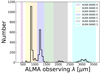 |
Fig. 1. Number of pointings as a function of observing wavelength in the A3COSMOS database. The wavelength ranges of the ALMA bands are plotted as color-shaded regions. The most populated bands are 6 and 7, with ∼2000 pointings. |
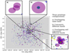 |
Fig. 2. Archival ALMA observations in the COSMOS field used in this study. Individual pointings are plotted with different colors representing the observed ALMA bands. In the background, the COSMOS field is shown in gray. We show three zoom-in regions representative of possible classes of pointing configurations. Panel a: three overlapping pointings in the same band. Panel b: three concentric pointings in different bands. Panel c: overlapping and concentric pointings in different bands. |
We selected galaxies above 4.35σ (with σ being the local RMS at the position of each source (see Adscheid et al., in prep.), and this selection yielded 1620 sources with flux in at least one ALMA band. For our sample, 25% (441/1620) of the sources have a spectroscopic redshift (spec-z), and for 1069 of the 1620 sources, we used the photo-z in the COSMOS2020 catalog. The spec-z in COSMOS2020 are from the literature (e.g., Riechers et al. 2013; Capak et al. 2015; Smolcic et al. 2015; Brisbin et al. 2017; Lee et al. 2017), the catalog by M. Salvato et al. (version 2017 September 1; available internally to the COSMOS collaboration), and the ALMA archive (Liu et al. 2019b). The photo-z used in this work are from Salvato et al. (2011), Davidzon et al. (2017), Delvecchio et al. (2017), Jin et al. (2018) and are derived from either the CLASSIC or FARMER version of the COSMOS2020 catalog. Finally, the remaining 110 of the 1620 sources do not have any redshift information. For this subsample, we computed their photo-z using CIGALE (Boquien et al. 2019) as described in the next section.
3. CIGALE SED fitting
We decided to perform the SED fitting of the A3COSMOS galaxies using CIGALE, a python SED-fitting code based on the energy balance between the UV and optical emission by stars and the re-emission in the IR and mm by the dust. As CIGALE is a highly flexible code, it allows one to choose among different individual templates for each emission component (e.g., stellar optical/UV emission, cold dust emission, active galactic nucleus) across a broad parameter space. Furthermore, one of the most important features is the availability of active galactic nucleus (AGN) templates, which can be easily included in the fit, allowing a decomposition between star formation-powered and AGN-powered IR emission. We note that deriving the IR luminosity from the SED is crucial to computing the IR LF.
In the following sections, we report the available photometry and the individual components used to perform the SED fitting following recent SED-based studies (Ciesla et al. 2017; Lo Faro et al. 2017; Małek et al. 2018; Pearson et al. 2018; Buat et al. 2019; Donevski et al. 2020). Moreover, when needed, we included an input grid of redshifts in the fit spanning between z = 0 and z = 8 (with a step of Δz = 0.1) in order to derive the best photo-z, if missing.
3.1. Photometric coverage
The A3C20 catalog, being a combination of the COSMOS2020 catalog and the archival ALMA observations, takes advantage of a large photometric coverage from the UV to the far infrared (FIR)/mm. To perform the SED fitting, we considered the following filters available in the COSMOS2020 catalog (Weaver et al. 2022): CFHT MegaCam u; Subaru Suprime-Cam i, B, V, r, and z; Subaru HSC y; VISTA VIRCAM Y, J, H, and Ks; and the superdeblended filters (Jin et al. 2018) Spitzer IRAC channel 1, 2, 3, and 4; Spitzer MIPS 24 μm; Herschel PACS at 100 and 160 μm; Herschel SPIRE at 250, 350, and 500 μm; JMCT SCUBA2 at 850 μm; ASTE AzTEC (1 mm); and IRAM MAMBO (1.2 mm).
To deal with all the ALMA frequency setup present in the A3COSMOS database, we built artificial filters to be provided to CIGALE, each corresponding to an observing wavelength in the A3COSMOS catalog. The filters are centered at a specific wavelength and are box-like, with their width being equal to 16 GHz. With this procedure, we added up to 330 continuous ALMA filters between 446 μm and 3325 μm to the CIGALE database.
3.2. CIGALE input templates
We modeled the stellar population with the bc03 stellar population synthesis model (Bruzual & Charlot 2003), to build the SED stellar component, and a delayed star formation history (SFH) with an optional second burst of star formation. We selected the dustatt_modified_CF00 (Charlot & Fall 2000) template to model the attenuation by dust and the dl2014 (Draine et al. 2014) to model the dust emission, both based on the assumption of having two different attenuation and emission sources represented by birth clouds and diffuse ISM.
Finally, we used the fritz2006 module (Fritz et al. 2006; Feltre et al. 2012) to model the AGN component in the SED. The AGN emission is described with a radiative transfer model, which takes into account primary emission coming from the central engine (i.e., the accretion disk), scattered emission produced by dust, and a thermal component of the dust emission. The individual input parameters are described in detail in Appendix A.
3.3. SED-fitting results
We performed the SED fitting for the 1620 sources of our sample using CIGALE with the modules described above. For our purposes, we obtained the following output parameters: dust luminosity (i.e., the IR 8–1000 μm luminosity), stellar mass, AGN fraction (fAGN) contributing to the 5 − 40 μm total emission, and τ (equatorial optical depth at 9.7 μm) and Ψ (angle between equatorial axis and line of sight) parameters of the fritz2006 model and redshift for 110 sources.
Among the 1620 sources for which we performed the fit, we first removed those presenting a high reduced χ2 (>10). Since our goals are strictly linked to the IR emission of these sources, we also computed the ratio between the ALMA observed flux and the best-fit flux at the same wavelength; sources with a ratio greater than the 5σ of the ratio distribution were removed and classified as “bad SED” if we were not able to reperform an acceptable fit. The 5σ threshold was selected in order to be consistent with the “good SED” selection performed by Liu et al. (2019b) and Adscheid et al. (in prep.) in the catalog construction. We obtained a good fit for 1411 of the 1620 galaxies, with 43 of 110 sources having no initial associated redshift. The remaining 67 galaxies without redshift had a bad fit (i.e., the IR-millimeter photometry did not match the optical part of the SED), so we decided to exclude them from the final sample, but we consider them in the incompleteness estimate. In Fig. 3 we show the best-fitting SED of three representative objects: a Type II AGN, a Type I AGN, and a galaxy without an AGN component.
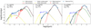 |
Fig. 3. Examples of SED-fitting results for three different classes of objects. From left to right: Unobscured AGN SED, SED without an AGN contribution, and obscured AGN component. The blue circles and the red triangles represent data points and upper limits, respectively. The best-fit model is plotted as a black solid line. The stellar attenuated and unattenuated, the dust emission, and the AGN emission are respectively reported as a yellow solid line, a blue dashed line, a red solid line, and a green solid line. |
In Fig. 4, we report the redshift distribution (top-left panel) of the sample as well as the results from the SED fitting for stellar mass (bottom left), dust luminosity (bottom right), and AGN fraction (top-right panel) for both the initial (1411) and final (189 after the cut; see Sect. 4) sample of galaxies. The redshift distribution peaks between z ∼ 1.5 and z ∼ 3.
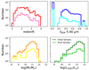 |
Fig. 4. Distributions of the main physical parameters obtained through SED fitting for the initial and final, reduced, sample. Top-left panel: redshift distribution. Top-right panel: AGN fraction distribution, computed in the 5–40 μm range. Bottom-left panel: logarithm of stellar mass distribution, in units of solar masses. Bottom-right panel: logarithm of the dust luminosity in solar luminosities. |
The galaxies in the sample are massive, with a peak in the distribution of stellar mass at log(M⋆/M⊙)∼11, consistent with them being DSFGs (Chapman et al. 2005; Simpson et al. 2014), although our sample contains sources with masses as low as 108 M⊙. The A3C20 galaxies are on average IR-bright, most of which have IR luminosities spanning from 1011 L⊙ to 1013 L⊙. Using the best-fitting templates for each source, we were able to compute the AGN luminosity in a given wavelength range and thus the fractional AGN contribution to the total emission in that range. The 5–40 μm range is particularly sensitive to the presence of an AGN. Therefore, we considered this wavelength interval to derive the fraction of AGN, fAGN, contributing to the luminosity in this range. As can be seen based on Fig. 4, the distribution is bimodal, and most of the sources (∼65%) have an AGN fraction near zero (i.e., they likely do not host an AGN), and the remainder have a fAGN higher than ∼0.2, peaking at ∼0.4, with a tail up to 0.8 − 0.9. The gap between fAGN = 0 and higher values is due to the grid we adopted for the SED fitting. Despite 35% of sources including an AGN component (the mean fAGN is ∼0.4) in the best-fit SED, only a small fraction (∼15%) is AGN dominated (i.e., fAGN > 0.5). Also, since the AGN emission is mostly present in the 5 − 40 μm range, the contribution to the 8 − 1000 μm emission is only a small fraction. For consistency with Gruppioni et al. (2013) and other SFRD estimates, we used the total (AGN+galaxy) IR emission, although we stress the AGN is strongly subdominant, and a more quantitative analysis is left to a future stand-alone work. For these reasons, we did not remove the AGN contribution from the total LIR.
Finally, we derived the dust-obscured SFR for each galaxy using the Kennicutt (1998) relation, which assumes the SFR to be proportional to the IR luminosity:
 (1)
(1)
We compare the SFR against stellar mass distribution (main sequence; MS) in Fig. 5. Our sample is characterized by star-forming galaxies with SFRs up to ∼103 M⊙ yr−1, typical of starbursting galaxies at the considered redshift. In each panel in the figure, we plot the MS from Speagle et al. (2014) computed at the mean redshift of the bin (solid black line) and an upper line (in dashed black line) corresponding to four times the MS, which is indicative of the starbursting regime (Rodighiero et al. 2011). Starburst galaxies tend to cluster on a “sequence” above and parallel to the MS, as also noted in other works (Caputi et al. 2017; Bisigello et al. 2018). As our SFR is derived directly from the IR luminosity, this bimodality cannot be simply explained with the parametrization of the SFH or the presence of dust, and the exact origin of this effect needs further investigation with additional data. However, in our case, the selection of Principal Investigators (PIs) can affect the MS distribution. In particular, we show in Fig. 5 the distribution of the sources on the MS plane before (1411 sources) and after (189 sources) removing the targeted sources (i.e., the target of the individual pointing) in blue and red. As can be noticed, the red circles mostly occupy the region on the MS.
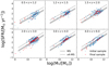 |
Fig. 5. Main sequence of galaxies computed in six different redshift bins: 0.5–1.2, 1.2–1.5, 1.5–2.0, 2.0–3.0, 3.0–4.0, 4.0–6.0. Data of the full sample are reported as blue circles, while the red diamonds represent the final sample (Sect. 4.4) used in our analysis. The black solid line and shaded area indicate the main sequence Speagle et al. (2014; computed at the mean values of the redshift bins) and 1σ dispersion. Finally, the black dashed lines represent the 4x MS, indicative of the starburst regime. |
Finally, for six out of 189 sources, we were unable to obtain a reasonable fit. The common characteristic of these sources is that they have an SED characterized by optical and ALMA photometry that does not appear to belong to the same object and can only be fitted by assuming extreme, unrealistic templates of dust emission. For this reason, and by inspecting the ALMA and optical cutouts, we decided to treat these sources statistically in the derivation of the LF. The details of the procedure, as well as some examples, are shown in Sect. 5.1.
4. Turning the A3C20 sample into a blind survey
The A3COSMOS survey is based on observations with different sensitivities (i.e., limiting fluxes), resolutions, and ALMA observed-frame wavelengths. The result is a survey of observations with unique selection functions. Being a collection of several observations, almost every pointing is centered on a targeted source of interest for that observation. In this perspective, the use of the A3COSMOS survey for statistical purposes (e.g., LF, SFRD) needs a dedicated analysis for turning it into a blind survey. In this section, we discuss the method we used to turn a generic (F)IR-millimeter ensemble of pointed observations into a blind survey (see also Adscheid et al., in prep.).
4.1. Blind surveys
To derive statistical properties of the sample through the corresponding areal coverage, a blind survey is needed. In order to achieve the construction of a blind survey, the next step should be followed and features fulfilled. In determining the limiting flux of A3COSMOS, we scaled the RMS of each individual pointing to the corresponding RMS at our reference wavelength of 1.2 mm (Sect. 4.2). We then determined the total area spanned by our survey, accounting for the primary beam attenuation and overlapping pointings (Sect. 4.3). Finally, any possible bias due to the presence of a target was taken into account (Sect. 4.4).
4.2. Root mean square conversion between different λobs
The first step in obtaining an unbiased survey from the A3COSMOS sample was the conversion of all observing wavelengths to a reference one. In our case, we chose the λref = 1200 μm wavelength in the observed frame, which falls in ALMA Band 6, as it is the most populated. This way, we could rescale all the fluxes at each observing wavelength (λobs) to a reference one (λref) using the fluxes at the observed SEDs in order to infer the observed ratio between λref and λobs for each source. In particular, we expected a decrease of the flux ratios when going to a higher z and shorter wavelengths, since the two fluxes approaches the rest-frame peak of dust emission in the SED.
As reported in Fig. 6, we divided the sample into five redshift bins (z < 1.5, 1.5–2.5, 2.5–3.5, 3.5–4.5, 4.5–6). For visualization purposes, we plotted only the most populated bands as gray circles. The colored points indicate the median value for a certain λobs for a specific redshift bin. It can be seen in the figure that for shorter λobs (close to λref), the ratios are unsurprisingly low and almost redshift independent, while at longer λobs the ratios become larger and more redshift dependent, especially in the highest z-bin.
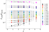 |
Fig. 6. Ratio between the flux at 1200 μm and other bands against redshift. The gray circles in the background indicate the values for individual sources in each band, while the colored circles refer to the median values in each redshift bin and for each ALMA band, as described in Sect. 4.2. |
Figure 7 shows the differences between the ratios in the different z-bins. We note that for z < 4.5, the correction curves are very similar to each other. For this reason, we used only one mean curve (up to z = 4.5) and a different one for z > 4.5 in our analysis.
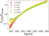 |
Fig. 7. Ratio between the flux at 1200 μm and in other bands against observed wavelength. Each circle is the median value computed as described in Sect. 4.2. The red, brown, gray, and yellow circles are at z < 4.5, while the green circles represent the last redshift bin at z > 4.5. |
4.3. Radial limiting flux
We used the conversion curves obtained as explained in the previous section to convert the RMS in each pointing as if it was observed at 1200 μm. Subsequently, the pointings became characterized by a uniform (in wavelength) sensitivity across their field of view (FoV). However, observing with the ALMA interferometer leads to a primary beam in which the sensitivity of the observation varies radially from the center to the outer regions.
For this reason, we divided the sky region covered by our pointings into 1″ pixels and flagged those inside a pointing with a flux value corresponding to the sensitivity of that pointing (i.e., primary beam correction higher than 0.2). We were then able to parametrize the primary beam correction (pbcor hereafter) as a Gaussian function peaking at the center of the circle with a value of one and decreasing to zero toward the outer regions:
 (2)
(2)
with d being the distance of a pixel from the center of the pointing and σ being the FWHM/2.35.
Working pixel by pixel and dividing the RMS by the pbcor corresponding to a pixel’s distance, we obtained a corrected RMS. We then converted the corrected RMS to the limiting flux by multiplying it by 4.35, which is the sensitivity cutoff of the prior catalog of A3COSMOS. After this procedure, we ended up with a pixel map of limiting fluxes inside the pointings. However, for the pointings that were overlapping, the selection of an exclusive area was not straightforward. Indeed, the common area between two overlapping pointings has to be counted only once, and the limiting flux from one of the two pointings needs to be assigned to the common area.
This issue has been dealt with by following the Avni & Bahcall (1980) method, which coherently combines multiple samples at different depths. As shown in Fig. 8, the limiting flux in the common area covered by two or more pointings is the one corresponding to the most sensitive observation at the reference frequency (i.e., the lowest limiting flux among the pointings).
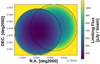 |
Fig. 8. Two overlapping pointings in band 6. The black circle represents the adopted primary beam size (out to a pbcor of 0.2), color-coded by the inferred RMS. Lower RMS values are represented by darker colors and higher values by lighter ones. Outside our primary beam boundary, we set values to the arbitrary high value of 106 μJy. In these types of cases, we adopted the area from the deepest pointing in the overlapping region. |
4.4. Areal coverage
We proceeded by deriving the cumulative areal coverage of our survey by combining the effective area accessible by all pointings at each limiting flux. This was done by counting the number of pixels with a certain limiting flux and deriving their cumulative distribution function. In this way, it would be possible to associate an area with a limiting flux (SLIM), which is the portion of area with a flux lower than SLIM.
In order to minimize potential biases due to pre-targeted ALMA sources contaminating the selection function, we disregarded central targets as follows. We removed pointings in which a target source was not present in the central 1″ (2060/3215). In this way, we took into account the possible positional offset of the SMG-galaxy follow-up with ALMA, which is of about 5″ and therefore could be wrongly addressed as a serendipitous detection. By removing pointings without a target, we were sure to not bias our sample with possible off-center targeted galaxies. The 1″ masking was chosen through a simulation varying the mask radius, increasing its size and comparing the retrieved masked number counts with an input distribution (Adscheid et al., prep.). It has been shown that when increasing the central mask radius, no benefit is observed in the convergence of the retrieved number counts. In addition, we also removed 104 of the 1620 sources that are potentially clustered (i.e., having a similar redshift to the target) following the criterion from Weaver et al. (2022), in which case a source can be considered to be at the same redshift of another if the difference in module between redshifts (zs and zt) is smaller than 0.04(1 + zt). Finally, we removed the target of each pointing.
The final sample, obtained by considering both the target and redshift cuts, consists of 189 sources from our initial sample of 1620 sources. We show in Fig. 9 the areal coverage for the remaining 1155 pointings (i.e., after removing pointings without a central target detection).
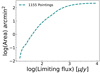 |
Fig. 9. Total areal coverage of the 1155 pointings after the cut for a lack of target detection within 1 arcsec. |
5. A3COSMOS luminosity function
Deriving the areal coverage of our survey allowed us to properly compute the luminosity function with the 1/VMAX method (Schmidt 1970). In the following sections, we describe the method applied to derive the total infrared luminosity function and compare it with previous works.
5.1. The method
We derived the LF using the Schmidt (1970) method that, based on the data, allowed us to derive the LF without making any assumption relative to the LF shape. As already mentioned in Sect. 4, the A3COSMOS survey is composed of approximately 1155 individual pointings (after the cut) that can be considered as independent fields. For this reason, by following the Avni & Bahcall (1980) method, we were able to derive the effective areal coverage at each SLIM across all pointings. We then used the relation between area and limiting fluxes (see Fig. 9) to associate an accessible area above a certain flux with each source.
To compute the LF, we divided our sample into eight redshift bins from z ∼ 0.5 to z ∼ 6 and into luminosity bins of 0.5 dex width from log(LIR/L⊙) = 10 to log(LIR/L⊙) = 14. For each source in a z-LIR bin, we measured the contribution to the LF in that bin by applying a redshift step of dz = 0.02 and K-correcting its SED from the lower to the upper boundary of the corresponding redshift bin, each time computing the observed flux at 1200 μm. We used this flux to infer the corresponding areal coverage at each dz by interpolating the previously derived areal coverage curve (Fig. 9). Lastly, we combined the effective area obtained in this way with the element of volume at each redshift step and obtained a co-moving volume over which a given source is accessible:
 (3)
(3)
where Vzmax and Vzmin are the sum of the subvolume in each dz shell up to the upper and lower limits of the bin, respectively. In particular, Vzmax can either be the volume at the upper bound of each dz bin or the maximum volume reachable by considering the S/N limit of the survey (i.e., corresponding to the z at which the area would be zero). Finally, we corrected the VMAX by taking into account the completeness and spuriousness corrections derived by Liu et al. (2019b), and we obtained the Φ(L, z) by summing each 1/VMAX in a certain luminosity-redshift bin.
5.2. Statistical treatment for potential HST-dark sources
As described in Sect. 3.3, we were unable to obtain a satisfactory fit for the SED of six of the 189 sources. Additionally, we identified these six sources as potential HST-dark objects. Consequently, due to having only ALMA flux information (the photo-z is associated with optical photometry), these objects were treated statistically in the LF analysis. Specifically, we assumed that these sources exist at a redshift greater than three, and we utilized the following procedure: First, we computed the cumulative redshift distribution for the rest of the sample. Next, for each Nth (N = 100) random extraction during the LF calculation, we assigned a redshift to each of the sources by drawing from the cumulative distribution function as a random sampler. Once a redshift was drawn, we used the median SED of the sample to “fit” the ALMA flux and consequently obtained an infrared luminosity to be incorporated into the LF calculation. Figure 10 shows an example for one of these sources, in which the ALMA emission (upper-left panel) is not observed with other instruments (acs-I, UV-j, IRAC1).
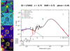 |
Fig. 10. Example of a source with optical identification (photo-z = 0.74) likely distinct from the ALMA galaxy. Left panel (from top to bottom): ALMA, acs-I, UV-j, and IRAC1 images are displayed with ALMA contours overlaid. It can be inferred that the optical/NIR object near the ALMA position is not centered in the ALMA galaxy. Right panel: SED of the same object showing the impossibility of fitting the optical and ALMA millimeter flux simultaneously. |
5.3. Infrared luminosity function
We obtained the IR LF by using the total (i.e., including all the SED components) LIR computed in the 8 − 1000 μm range. The z-bins (0.5–1.0; 1.0–1.5; 1.5–2.0; 2.0–2.5; 2.5–3.0; 3.0–3.5; 3.5–4.5; 4.5–6.0) are nearly equally populated, apart from the first bin, which contains slightly fewer sources than the others. The LF is shown in Fig. 11 as black circles, and the red boxes represent the Poissonian uncertainties, and the values are reported in Table 1. In each panel, we have overplotted the completeness limit as a vertical black dashed line. This threshold was computed by rescaling all the observed 1200 μm fluxes of each SED to the same limiting flux and then taking the LIR of the SED, which gave the highest LIR value at that limit. This latter value represents the value of LIR below which our sample is not 100% complete. The points below the completeness limit are reported as white boxes (with red borders) in Fig. 11. We also report existing estimates obtained from other studies. In particular, we compared our results with the best fit from previous IR works, either from ALMA (ALPINE; Gruppioni et al. 2020) or Herschel (PEP+GOODS-H and PEP+HerMES; Magnelli et al. 2013; Gruppioni et al. 2013), when available for redshifts that are similar to ours.
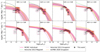 |
Fig. 11. A3COSMOS luminosity function (black circles and red boxes). The individual redshift bin MCMC best fit is plotted as pink solid lines and shaded error bands. The redshift ranges are reported in the upper-right corner of each subplot, while the luminosity bins are centered at each 0.25 dex, with a width of 0.5 dex (overlapping bins). The black vertical dashed lines represent the completeness limit of the LIR. The orange dashed, purple dotted, and green dashed lines are the best-fit LFs obtained by Gruppioni et al. (2013, 2020), Magnelli et al. (2013). |
Infrared luminosity function as inferred using the A3COSMOS database.
As can be seen from Fig. 11, we mostly sampled the bright end of the luminosity function, as our complete points are above log(LIR/L⊙) ≃ 12 at each redshift bin. This is mainly a consequence of the fact that, at lower redshift, ALMA samples down the Rayleigh-Jeans tail, and therefore even if deep pointings are available, they are inefficient compared to Herschel, which samples the peak of the IR SED. The peak of dust emission can be better probed by ALMA (Band 6 and 7 mainly) at high redshifts (z > 3). Despite this, our data points are in good agreement, within the errors, with the black triangles from Herschel (see Fig. 12), whose z < 3 LF estimates are characterized by much higher statistics (smaller error bars) and better sensitivity and are thus able probe the IR LF down to the faint end and the knee region (log(LIR/L⊙) ≃ 11). From this consistency with the LF from Gruppioni et al. (2013), we can assert that despite the poorer statistics in terms of the number of sources, the method used to turn the A3COSMOS into a blind survey is valid and accurate. At z > 3 − 3.5, where Herschel probes further down the peak of the dust emission and ALMA starts probing the peak, our estimates show a systematically higher normalization. Indeed, as stated by Gruppioni et al. (2013), in the 3 < z < 4.2 Herschel redshift bin, most of the sources have a photometric redshift, and the PEP selection may be missing a fraction of high redshift galaxies, making this estimate a lower limit.
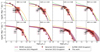 |
Fig. 12. A3COSMOS (red boxes and black circles) + Herschel (black triangles) luminosity function. The dark-red lines and shaded areas are the best fit obtained by using all the LF points from different z-bins together. The redshift ranges are reported in the upper-right corner of each subplot, while the luminosity bins are centered at each 0.25 dex, with a width of 0.5 dex (overlapping bins). The black vertical dashed lines represent the completeness limit of the LIR. The orange dashed, purple dotted, and green dashed lines are the best-fit LFs obtained by Gruppioni et al. (2013, 2020), Magnelli et al. (2013). |
5.4. Luminosity function best fit and evolution
To trace the number density of galaxies at different redshifts and IR luminosities, we quantified the LF using a Schechter function. For this purpose, we modeled our LF with a modified Schechter function (Saunders et al. 1990) described by four free parameters:
![Mathematical equation: $$ \begin{aligned} \Phi (L)d\log L = \Phi ^*\left(\frac{L}{L^*}\right)^{1-\alpha _S} \exp \left[-\frac{1}{2\sigma _S^2}\log _{10}^2 \left(1+\frac{L}{L^*}\right)\right]d \log L, \end{aligned} $$](/articles/aa/full_html/2024/01/aa47048-23/aa47048-23-eq4.gif) (4)
(4)
where αS and σS are the slope of the faint end and the parameter shaping the bright-end slope, respectively, and L* and Φ* represent the luminosity and normalization at the knee, respectively. The modified Schechter function is similar to a power law for L ≪ L* and behaves as a Gaussian for L ≫ L*.
To find the L* and Φ* that best reproduce our LF, we performed a Markov chain Monte Carlo (MCMC) analysis using the PYTHON package emcee (Foreman-Mackey et al. 2013), which uses a set of walkers to explore the parameter space simultaneously. We carried out the MCMC analysis using 50 walkers with 10 000 steps (draws), discarding the first 1000 sampled draws of each walker (burnin). The likelihood was built in the following form:
 (5)
(5)
We ran the MCMC using flat prior distributions for the two free parameters and with αS and σS fixed to the values of Gruppioni et al. (2013; i.e., αS = 1.2 and σS = 0.5), with log(Φ*) between −5 and −2 and log(L*) between 10 and 13. The prior distribution was then combined with the likelihood function to obtain the posterior distribution.
We fitted the ALMA points alone (Fig. 11) in the lower redshift bins (i.e., 0.5 < z < 1.0 and 1.0 < z < 1.5). The individual fit showed a very low normalization with respect to the Herschel best-fit and large error bands, and it did not allow us to constrain the fit parameters L* and Φ* in an accurate way. Between redshift 1.5 and 3.0, the best-fit LF is in good agreement with Herschel, except for a slightly higher but consistent normalization in the 1.5 < z < 2.0 redshift bin. Finally, between z = 3 and z = 3.5, our best fit is consistent with that of the ALPINE survey (Le Fèvre et al. 2020) but has lower Φ* at the knee at z > 3.5.
Since the ALMA-only LF (Fig. 12, red boxes) is not able to trace the lowest luminosities, we decided to take advantage of the great number of statistics and coverage in luminosity of the PEP+HerMES survey by Herschel (Gruppioni et al. 2013) up to z ∼ 3, with which our sample is consistent, while extending to higher redshift using our ALMA measurements. By means of this approach, it became possible to better characterize the faint end and the knee of the LF at z > 3. Indeed, by using Herschel’s LF data at all available redshifts (in Fig. 12, only those within the redshift bins from 0.5 to 6 are shown), the MCMC analysis we conducted managed to characterize the parameters of the Schechter function better and subsequently trace its evolution at higher z.
Previous works already pointed toward a redshift evolution of both a typical density and luminosity of the IR galaxy population (see e.g., Caputi et al. 2007; Béthermin et al. 2011; Marsden et al. 2011; Gruppioni et al. 2013) characterized by an increase in luminosity and a decrease in density with increasing redshift. In particular, both Caputi et al. (2007), Béthermin et al. (2011) and Gruppioni et al. (2013) found a break in the redshift evolution resulting in a steepening of the density evolution a z > 1 and a flattening for the luminosity at z > 2. For these reasons, we performed a second MCMC fit using the multiredshift information from each redshift bin, assuming an exponential shape and two different zbreak values (zρ0 and zl0) for the evolution of Φ(z)* and L(z)*, expressed as:
 (6)
(6)
 (7)
(7)
where  and
and  are the normalization and characteristic luminosity at z = 0 and kρ1, kρ2, kl1, and kl2 are the exponents for values lower and greater than zρ0 and zl0 for Φ and L, respectively. In this second fit, each point of the LF is associated with a redshift corresponding to the median value of the galaxy population inside the individual redshift bin. By using these values, we could trace a more accurate evolution of Φ* and L*. From this fit, we obtained two evolution curves (L* and Φ* versus z) that take into account the shape of the LF at each z. The priors used in this MCMC are given for the parameters that regulate the evolution of the LF, while αS and σS are fixed to 1.2 and 0.5 (found by Gruppioni et al. (2013) at z ∼ 0.15) and anchor Φ* and L* to their value at z ∼ 0.7 found with Herschel-only measurements. In particular, we fixed the L* and Φ* at z ∼ 0.7 to be the same found by Herschel. The best-fit curve at each z-bin is shown in Fig. 12 as a dark-red solid line and shaded errors.
The trend with the redshift of L* and Φ* is reported in Fig. 13, and the results of the MCMC fit are reported in Tables 2 and 3, representing the 16th and 84th percentiles’ error bands and the best-fit values at z = 0. The curve from the evolutionary MCMC and uncertainties are reported as dark-red lines and shaded areas. For comparison, the estimates of the individual fit are plotted as pink diamonds for the ALMA-only case. From Fig. 13, it is possible to observe that the values of L* and Φ* estimated by fitting only the A3COSMOS data points are slightly inconsistent with the results obtained using A3COSMOS plus Herschel (at z > 2). As mentioned before, this is due to the limited ability of ALMA to trace the dust peak emission at z < 2 and to the larger weight of Herschel data (containing more sources) in the combination. The evolution of Φ changes from  to lower values, with an evolutionary trend of Φ* ∝ (1 + z)−0.55 for z < zρ0 and Φ* ∝ (1 + z)−3.41 for z > zρ0. Overall, a decreasing trend was observed. This can be interpreted as a decreasing density of the bulk of star-forming galaxies at a given redshift. Notably, L* shows two different trends with redshift below and above the break. In particular, for
  , the L* evolves as (1 + z)3.41 and as L* ∝ (1 + z)0.59 for z > zl0, thus becoming flatter. The evolutionary trend of L* can be ascribed to downsizing (Thomas et al. 2010), that is, brighter (massive, according to the SFR − M relation) galaxies formed earlier than their fainter counterparts. A similar analysis has already been performed by Gruppioni et al. (2013) using the Herschel PEP/HerMES LF (indicated with black empty circles in Fig. 13), and they found a consistently decreasing Φ* and increasing L*. However, their value of zl0 (i.e., zl0 ∼ 2) is lower than what we obtained (zl0 ∼ 3). The evolution is in very good agreement with the Herschel-only results (empty black circles) and with the ALPINE estimates at z > 4.
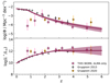 |
Fig. 13. Evolutionary trends of Φ* (top panel) and L* (bottom panel) with redshift. The solid dark-red lines and shaded areas show the behaviors of Φ* and L* at all the redshifts, while the pink diamonds are the estimates obtained when fitting each redshift bin individually in the ALMA-only case. Finally, the empty black circles and yellow circles represent estimates for L* and Φ* from Gruppioni et al. (2013, 2020), which we include for comparison. |
Best-fit parameters at the knee of the IR-LF.
MCMC results from the combined A3COSMOS and Herschel evolutive fit.
6. Dust-obscured star formation rate density
Finally, using the best-fit luminosity function in each redshift bin, we derived the co-moving SFRD. In particular, we first obtained the IR luminosity density (ρIR) by integrating the IR LF in each z bin from log(LIR) = 8 (to be consistent with other IR-based SFRDs) to log(LIR) = 14:
 (8)
(8)
Then, we could convert the IR luminosity density into a SFRD by applying the Kennicutt (1998) relation to convert LIR to SFR, assuming a Chabrier (2003) IMF. As described in Sect. 5.4, in addition to the individual fit, we performed an MCMC fitting taking the information from all the redshift bins together in order to derive the redshift evolution of L* and Φ*. In this way, we obtained the LF at each redshift from z ∼ 0.5 to z ∼ 6, and we integrated the LF[L*(z),Φ*(z)] in the full redshift range (for clarity, we report the results of the fit for the eight bins of our IR LF). The result was an evolution curve of the SFRD with the redshift, shown in Fig. 14. The values of the SFRD and error bands are reported in Table 4. The dark-red solid lines with the shaded area represent the lower and upper boundaries of the curve derived as the errors on the integration of the LF at each redshift. In order to compare our values with those from the literature, we have overplotted previous results on the SFRD from Madau & Dickinson (2014), Béthermin et al. (2017), Lagache (2018) and from the IllustrisTNG simulation (Pillepich et al. 2018) in the figure. Estimates of the dust-obscured SFRD from other IR-millimeter works (Gruppioni et al. 2013, 2015, 2020; Magnelli et al. 2013; Rowan-Robinson et al. 2016; Liu et al. 2018) are reported as empty red circles with different markers. The empty blue circles represent the SFRD from UV works, corrected from dust attenuation, by Dahlen et al. (2007), Reddy & Steidel (2009), Cucciati et al. (2012), Bouwens et al. (2012, 2015).
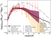 |
Fig. 14. Co-moving SFRD evolution with z. The red diamonds were obtained through the integration of the LF best-fit in each z bin, while the dark-red shaded area was obtained by integrating the evolutionary LF from z= 0.5 to 6. Comparison curves from the literature are reported as gray dash-dotted (pessimistic and optimistic cases; Lagache 2018); dashed (IllustrisTNG), dotted (Béthermin et al. 2017), and black solid lines (Madau & Dickinson 2014). The empty red circles with different symbols represent different IR-millimeter estimates of the SFRD from Gruppioni et al. (2013, 2015, 2020), Magnelli et al. (2013), Rowan-Robinson et al. (2016), Liu et al. (2018), and the orange shaded area is the dust-obscured SFRD by Zavala et al. (2021), from the MORA survey. The SFRD from the UV is plotted as empty blue circles with different markers (Dahlen et al. 2007; Reddy & Steidel 2009; Cucciati et al. 2012; Bouwens et al. 2012, 2015). |
Star formation rate density obtained by integrating the LF best-fit in our eight redshift bins.
Thanks to the use of the Herschel data points, combined with the ALMA ones, in the LF fit, we were able to derive accurate estimates of the dust-obscured SFRD also at z < 3. We found the SFRD computed at z ∼ 0.5 − 1.0 follows the rise described by Madau & Dickinson (2014; dark gray curve) and is consistent with the IR and UV estimates from previous works. Although our points up to z ∼ 2 have a lower normalization with respect to those from Gruppioni et al. (2013) and Magnelli et al. (2013), this discrepancy may be explained by the different types of fit performed, which results in a different extrapolation to the faint end. From z ∼ 2 to z ∼ 3.5, the SFRD follows a flat trend, being above the Madau & Dickinson (2014). This flattening of the SFRD is compatible with predictions from models that envisage the early formation of massive spheroids (see Calura & Matteucci 2003). As mentioned before, at z > 3, our estimates were derived using ALMA alone (last three redshift bins). The observed trend is a decrease of the dust-obscured SFRD up to z ∼ 6, even though the limited number of sources does not allow us to strictly constrain it at those redshifts. We found the z > 3 dust-obscured SFRD to be consistent with the dust-corrected UV estimates and with the estimate of Madau & Dickinson (2014), while in the lower boundary, we found it to be consistent with the dust-obscured SFRD derived by Zavala et al. (2021), although with a ∼0.5 dex difference between the mean values. The upper boundary is consistent with Gruppioni et al. (2020), pointing toward a possibly underestimated SFRD at z > 3. However, this underestimation seems not to be as extreme as suggested by Rowan-Robinson et al. (2016) and Gruppioni et al. (2020).
7. Summary and conclusions
Owing to the photometric coverage of COSMOS2020 + ALMA, we were able to perform SED fittings using the CIGALE code to constrain the SFR, LIR, and M⋆ of the full ALMA sample. Applying the Avni & Bahcall (1980) method, we were able to reconcile the overlapping regions between several pointings and correctly evaluate the depth of such regions. Moreover, we derived an SED-based method to homogenize the pointings at different observing wavelengths, converting the RMS noise into that of the reference wavelength. By removing pointings without a detected target and by correcting for clustering, we were able to turn A3COSMOS into an untargeted, “blind-like” survey. We thus derived the total infrared luminosity function in the 8 − 1000 μm band using the 1/VMAX (Schmidt 1970) method and using the already available data from Herschel. We estimated the LF from z ∼ 0.5 to z ∼ 6 and performed an MCMC simulation to fit the LF data, including the possibility for the characteristic parameters (Φ* and L*) to evolve with redshift. By integrating the LF, we derived the infrared luminosity density and thus the dust-obscured SFRD up to z ∼ 6. We summarize the conclusions of this work as follows:
-
We find the A3COSMOS sample to be characterized by galaxies that are massive (log(M⋆/M⊙) = 10 − 12) and bright in the IR (8 − 1000 μm) band, with log(LIR/L⊙) = 11 − 13.5. Converting LIR into SFR, we obtained values typical of normal star-forming (SFR ∼ 1 − 100 M⊙ yr−1) and starbursting galaxies (SFR ∼ 100 − 1000 M⊙ yr−1).
-
We find our LF to be in good agreement with the existing literature (in particular at z > 1), though it pushes the SFRD to z ∼ 6 with unprecedented statistics.
-
Our MCMC analysis suggests a joint redshift-decreasing number density and a redshift-increasing IR luminosity for ALMA-selected star-forming galaxies. This result is consistent with these galaxies being less frequent and more luminous (i.e., massive) when going toward higher redshift.
-
Our estimates of the dust-obscured SFRD are consistent with those from other IR surveys and with the UV dust-corrected estimates. Also, we found a broader peak in the SFRD, with a smooth decrease at z > 4, which suggests a significant contribution from the obscured SFRD at high redshift. Furthermore, a contribution to the SFRD, particularly at high redshifts, could originate from HST-dark sources (Simpson et al. 2014; Franco et al. 2018; Wang et al. 2019; Talia et al. 2021; Enia et al. 2022; Behiri et al. 2023), which are not, a priori, included in a prior sample, with the exception of the six added sources.
Our study of the physical (i.e., stellar mass, dust luminosity, star formation rate) and statistical (LF and SFRD) properties of the ALMA sample of galaxies in the COSMOS field resulted in the detection and characterization of a star-forming and starbursting dominated population, ∼40% of which likely host an AGN. We also found the A3C20 sample evolves both in luminosity (L*) and density (Φ*) and significantly contributes to the total (IR+UV) SFRD also at z > 3. However, in order to improve our knowledge and put tighter constraints on the evolution and formation of galaxies at higher z, more statistics are needed. Being constantly updated, the A3COSMOS catalog represents a key survey for reaching newer results with better statistics. With JWST, the future COSMOS-Web survey (Casey et al. 2023) will also play an important role in covering the COSMOS field, allowing surveys to obtain better photometric coverage and thus allowing the physical properties of galaxies to be better constrained.
Acknowledgments
I.D. acknowledges support from INAF Minigrant “Harnessing the power of VLBA towards a census of AGN and star formation at high redshift”. L.B. acknowledges the support from grant PRIN MIUR 2017 − 20173ML3WW_001. E.S. acknowledges funding from the European Research Council (ERC) under the European Union’s Horizon 2020 research and innovation programme (grant agreement No. 694343). This work was supported by NAOJ ALMA Scientific Research Grant Code 2021-19A (HA). S.G. acknowledges financial support from the Villum Young Investigator grant 37440 and 13160 and the Cosmic Dawn Center (DAWN), funded by the Danish National Research Foundation (DNRF) under grant No. 140. A.T. acknowledges G. Mazzolari and A. della Croce for all the useful discussions and N. Borghi, L. Leuzzi and C. Perfetti for all the support during the writing of this article.
References
- Aihara, H., AlSayyad, Y., Ando, M., et al. 2019, PASJ, 71, 114 [Google Scholar]
- Algera, H., Inami, H., Oesch, P., et al. 2023, MNRAS, 518, 6142 [Google Scholar]
- Aretxaga, I., Wilson, G. W., Aguilar, E., et al. 2011, MNRAS, 415, 3831 [Google Scholar]
- Avni, Y., & Bahcall, J. N. 1980, ApJ, 235, 694 [NASA ADS] [CrossRef] [Google Scholar]
- Barger, A. J., Cowie, L. L., Sanders, D. B., et al. 1998, Nature, 394, 248 [Google Scholar]
- Behiri, M., Talia, M., Cimatti, A., et al. 2023, ApJ, 957, 63 [NASA ADS] [CrossRef] [Google Scholar]
- Bertoldi, F., Carilli, C., Aravena, M., et al. 2007, ApJS, 172, 132 [Google Scholar]
- Béthermin, M., Dole, H., Lagache, G., Le Borgne, D., & Penin, A. 2011, A&A, 529, A4 [Google Scholar]
- Béthermin, M., Daddi, E., Magdis, G., et al. 2015, A&A, 573, A113 [Google Scholar]
- Béthermin, M., Wu, H.-Y., Lagache, G., et al. 2017, A&A, 607, A89 [Google Scholar]
- Bisigello, L., Caputi, K. I., Grogin, N., & Koekemoer, A. 2018, A&A, 609, A82 [NASA ADS] [CrossRef] [EDP Sciences] [Google Scholar]
- Blain, A. W., Smail, I., Ivison, R. J., Kneib, J. P., & Frayer, D. T. 2002, Phys. Rep., 369, 111 [Google Scholar]
- Boquien, M., Burgarella, D., Roehlly, Y., et al. 2019, A&A, 622, A103 [NASA ADS] [CrossRef] [EDP Sciences] [Google Scholar]
- Bouwens, R. J., Illingworth, G. D., Oesch, P. A., et al. 2012, ApJ, 754, 83 [Google Scholar]
- Bouwens, R. J., Bradley, L., Zitrin, A., et al. 2014, ApJ, 795, 126 [Google Scholar]
- Bouwens, R. J., Illingworth, G. D., Oesch, P. A., et al. 2015, ApJ, 803, 34 [Google Scholar]
- Bouwens, R. J., Aravena, M., Decarli, R., et al. 2016, ApJ, 833, 72 [NASA ADS] [CrossRef] [Google Scholar]
- Brisbin, D., Miettinen, O., Aravena, M., et al. 2017, A&A, 608, A15 [NASA ADS] [CrossRef] [EDP Sciences] [Google Scholar]
- Bruzual, G., & Charlot, S. 2003, MNRAS, 344, 1000 [NASA ADS] [CrossRef] [Google Scholar]
- Buat, V., Ciesla, L., Boquien, M., Małek, K., & Burgarella, D. 2019, A&A, 632, A79 [NASA ADS] [CrossRef] [EDP Sciences] [Google Scholar]
- Calura, F., & Matteucci, F. 2003, ApJ, 596, 734 [NASA ADS] [CrossRef] [Google Scholar]
- Capak, P., Aussel, H., Ajiki, M., et al. 2007, ApJS, 172, 99 [Google Scholar]
- Capak, P. L., Carilli, C., Jones, G., et al. 2015, Nature, 522, 455 [NASA ADS] [CrossRef] [Google Scholar]
- Caputi, K. I., Lagache, G., Yan, L., et al. 2007, ApJ, 660, 97 [NASA ADS] [CrossRef] [Google Scholar]
- Caputi, K. I., Deshmukh, S., Ashby, M. L. N., et al. 2017, ApJ, 849, 45 [Google Scholar]
- Casey, C. M., Narayanan, D., & Cooray, A. 2014, Phys. Rep., 541, 45 [Google Scholar]
- Casey, C. M., Zavala, J. A., Spilker, J., et al. 2018, ApJ, 862, 77 [Google Scholar]
- Casey, C. M., Kartaltepe, J. S., Drakos, N. E., et al. 2023, ApJ, 954, 31 [NASA ADS] [CrossRef] [Google Scholar]
- Chabrier, G. 2003, PASP, 115, 763 [Google Scholar]
- Chapman, S. C., Blain, A. W., Ivison, R. J., & Smail, I. R. 2003, Nature, 422, 695 [NASA ADS] [CrossRef] [Google Scholar]
- Chapman, S. C., Blain, A. W., Smail, I., & Ivison, R. J. 2005, ApJ, 622, 772 [NASA ADS] [CrossRef] [Google Scholar]
- Charlot, S., & Fall, S. M. 2000, ApJ, 539, 718 [Google Scholar]
- Ciesla, L., Elbaz, D., & Fensch, J. 2017, A&A, 608, A41 [NASA ADS] [CrossRef] [EDP Sciences] [Google Scholar]
- Civano, F., Elvis, M., Brusa, M., et al. 2012, ApJS, 201, 30 [Google Scholar]
- Civano, F., Marchesi, S., Comastri, A., et al. 2016, ApJ, 819, 62 [Google Scholar]
- Cucciati, O., Tresse, L., Ilbert, O., et al. 2012, A&A, 539, A31 [NASA ADS] [CrossRef] [EDP Sciences] [Google Scholar]
- da Cunha, E., Walter, F., Smail, I. R., et al. 2015, ApJ, 806, 110 [Google Scholar]
- Dahlen, T., Mobasher, B., Dickinson, M., et al. 2007, ApJ, 654, 172 [Google Scholar]
- Davidzon, I., Ilbert, O., Laigle, C., et al. 2017, A&A, 605, A70 [NASA ADS] [CrossRef] [EDP Sciences] [Google Scholar]
- Delvecchio, I., Smolčić, V., Zamorani, G., et al. 2017, A&A, 602, A3 [NASA ADS] [CrossRef] [EDP Sciences] [Google Scholar]
- Donevski, D., Lapi, A., Małek, K., et al. 2020, A&A, 644, A144 [NASA ADS] [CrossRef] [EDP Sciences] [Google Scholar]
- Draine, B. T., Aniano, G., Krause, O., et al. 2014, ApJ, 780, 172 [Google Scholar]
- Dudzevičiūtė, U., Smail, I., Swinbank, A. M., et al. 2020, MNRAS, 494, 3828 [Google Scholar]
- Elvis, M., Civano, F., Vignali, C., et al. 2009, ApJS, 184, 158 [Google Scholar]
- Enia, A., Talia, M., Pozzi, F., et al. 2022, ApJ, 927, 204 [NASA ADS] [CrossRef] [Google Scholar]
- Feltre, A., Hatziminaoglou, E., Fritz, J., & Franceschini, A. 2012, MNRAS, 426, 120 [Google Scholar]
- Foreman-Mackey, D., Hogg, D. W., Lang, D., & Goodman, J. 2013, PASP, 125, 306 [Google Scholar]
- Franco, M., Elbaz, D., Béthermin, M., et al. 2018, A&A, 620, A152 [NASA ADS] [CrossRef] [EDP Sciences] [Google Scholar]
- Fritz, J., Franceschini, A., & Hatziminaoglou, E. 2006, MNRAS, 366, 767 [Google Scholar]
- Fujimoto, S., Ouchi, M., Shibuya, T., & Nagai, H. 2017, ApJ, 850, 83 [Google Scholar]
- Geach, J. E., Dunlop, J. S., Halpern, M., et al. 2017, MNRAS, 465, 1789 [Google Scholar]
- Ginsburg, A., Sipőcz, B. M., Brasseur, C. E., et al. 2019, AJ, 157, 98 [Google Scholar]
- Gruppioni, C., Pozzi, F., Rodighiero, G., et al. 2013, MNRAS, 432, 23 [Google Scholar]
- Gruppioni, C., Calura, F., Pozzi, F., et al. 2015, MNRAS, 451, 3419 [Google Scholar]
- Gruppioni, C., Béthermin, M., Loiacono, F., et al. 2020, A&A, 643, A8 [NASA ADS] [CrossRef] [EDP Sciences] [Google Scholar]
- Harikane, Y., Nakajima, K., Ouchi, M., et al. 2024, ApJ, 960, 56 [NASA ADS] [CrossRef] [Google Scholar]
- Hodge, J. A., Karim, A., Smail, I., et al. 2013, ApJ, 768, 91 [Google Scholar]
- Hsieh, B.-C., Wang, W.-H., Hsieh, C.-C., et al. 2012, ApJS, 203, 23 [NASA ADS] [CrossRef] [Google Scholar]
- Hughes, D. H., Serjeant, S., Dunlop, J., et al. 1998, Nature, 394, 241 [Google Scholar]
- Ilbert, O., Capak, P., Salvato, M., et al. 2009, ApJ, 690, 1236 [NASA ADS] [CrossRef] [Google Scholar]
- Ilbert, O., McCracken, H. J., Le Fèvre, O., et al. 2013, A&A, 556, A55 [NASA ADS] [CrossRef] [EDP Sciences] [Google Scholar]
- Jin, S., Daddi, E., Liu, D., et al. 2018, ApJ, 864, 56 [Google Scholar]
- Kennicutt, R. C., Jr 1998, ARA&A, 36, 189 [NASA ADS] [CrossRef] [Google Scholar]
- Khusanova, Y., Bethermin, M., Le Fèvre, O., et al. 2021, A&A, 649, A152 [NASA ADS] [CrossRef] [EDP Sciences] [Google Scholar]
- Lagache, G. 2018, in Peering towards Cosmic Dawn, eds. V. Jelić, & T. van der Hulst, 333, 228 [NASA ADS] [Google Scholar]
- Laigle, C., McCracken, H. J., Ilbert, O., et al. 2016, ApJS, 224, 24 [Google Scholar]
- Lang, D., Hogg, D. W., & Mykytyn, D. 2016, Astrophysics Source Code Library [record ascl:1604.008] [Google Scholar]
- Laporte, N., Infante, L., Troncoso Iribarren, P., et al. 2016, ApJ, 820, 98 [NASA ADS] [CrossRef] [Google Scholar]
- Leauthaud, A., Massey, R., Kneib, J.-P., et al. 2007, ApJS, 172, 219 [NASA ADS] [CrossRef] [Google Scholar]
- Lee, G. H., Hwang, H. S., Sohn, J., & Lee, M. G. 2017, ViZieR Online Data Catalog: J/ApJ/835/280 [Google Scholar]
- Le Fèvre, O., Béthermin, M., Faisst, A., et al. 2020, A&A, 643, A1 [Google Scholar]
- Le Floc’h, E., Aussel, H., Ilbert, O., et al. 2009, ApJ, 703, 222 [Google Scholar]
- Liu, D., Daddi, E., Dickinson, M., et al. 2018, ApJ, 853, 172 [Google Scholar]
- Liu, D., Schinnerer, E., Groves, B., et al. 2019a, Astrophysics Source Code Library [record ascl:1910.003] [Google Scholar]
- Liu, D., Schinnerer, E., Groves, B., et al. 2019b, ApJ, 887, 235 [Google Scholar]
- Lo Faro, B., Buat, V., Roehlly, Y., et al. 2017, MNRAS, 472, 1372 [NASA ADS] [CrossRef] [Google Scholar]
- Lutz, D., Poglitsch, A., Altieri, B., et al. 2011, A&A, 532, A90 [NASA ADS] [CrossRef] [EDP Sciences] [Google Scholar]
- Madau, P., & Dickinson, M. 2014, ARA&A, 52, 415 [Google Scholar]
- Magdis, G. E., Daddi, E., Béthermin, M., et al. 2012, ApJ, 760, 6 [NASA ADS] [CrossRef] [Google Scholar]
- Magnelli, B., Lutz, D., Santini, P., et al. 2012, A&A, 539, A155 [NASA ADS] [CrossRef] [EDP Sciences] [Google Scholar]
- Magnelli, B., Popesso, P., Berta, S., et al. 2013, A&A, 553, A132 [NASA ADS] [CrossRef] [EDP Sciences] [Google Scholar]
- Małek, K., Buat, V., Roehlly, Y., et al. 2018, A&A, 620, A50 [Google Scholar]
- Marchesi, S., Civano, F., Elvis, M., et al. 2016, ApJ, 817, 34 [Google Scholar]
- Marsden, G., Chapin, E. L., Halpern, M., et al. 2011, MNRAS, 417, 1192 [NASA ADS] [CrossRef] [Google Scholar]
- McCracken, H. J., Capak, P., Salvato, M., et al. 2010, ApJ, 708, 202 [NASA ADS] [CrossRef] [Google Scholar]
- McCracken, H. J., Milvang-Jensen, B., Dunlop, J., et al. 2012, A&A, 544, A156 [NASA ADS] [CrossRef] [EDP Sciences] [Google Scholar]
- McMullin, J. P., Waters, B., Schiebel, D., Young, W., & Golap, K. 2007, ASP Conf. Ser., 376, 127 [Google Scholar]
- Mohan, N., & Rafferty, D. 2015, Astrophysics Source Code Library [record ascl:1502.007] [Google Scholar]
- Moneti, A., McCracken, H. J., Hudelot, W., et al. 2023, ViZieR Online Data Catalog: II/373 [Google Scholar]
- Muzzin, A., Marchesini, D., Stefanon, M., et al. 2013, ApJS, 206, 8 [Google Scholar]
- Oesch, P. A., Bouwens, R. J., Illingworth, G. D., et al. 2015, ApJ, 808, 104 [Google Scholar]
- Oesch, P. A., Bouwens, R. J., Illingworth, G. D., Labbé, I., & Stefanon, M. 2018, ApJ, 855, 105 [Google Scholar]
- Oliver, S. J., Bock, J., Altieri, B., et al. 2012, MNRAS, 424, 1614 [NASA ADS] [CrossRef] [Google Scholar]
- Pearson, W. J., Wang, L., Hurley, P. D., et al. 2018, A&A, 615, A146 [NASA ADS] [CrossRef] [EDP Sciences] [Google Scholar]
- Peng, C. Y., Ho, L. C., Impey, C. D., & Rix, H.-W. 2002, AJ, 124, 266 [Google Scholar]
- Peng, C. Y., Ho, L. C., Impey, C. D., & Rix, H.-W. 2010, AJ, 139, 2097 [Google Scholar]
- Pillepich, A., Nelson, D., Hernquist, L., et al. 2018, MNRAS, 475, 648 [Google Scholar]
- Reddy, N. A., & Steidel, C. C. 2009, ApJ, 692, 778 [Google Scholar]
- Riechers, D. A., Bradford, C. M., Clements, D. L., et al. 2013, Nature, 496, 329 [Google Scholar]
- Rodighiero, G., Daddi, E., Baronchelli, I., et al. 2011, ApJ, 739, L40 [Google Scholar]
- Rowan-Robinson, M., Oliver, S., Wang, L., et al. 2016, MNRAS, 461, 1100 [Google Scholar]
- Salvato, M., Ilbert, O., Hasinger, G., et al. 2011, ApJ, 742, 61 [Google Scholar]
- Sanders, D. B., Salvato, M., Aussel, H., et al. 2007, ApJS, 172, 86 [Google Scholar]
- Saunders, W., Rowan-Robinson, M., Lawrence, A., et al. 1990, MNRAS, 242, 318 [Google Scholar]
- Schinnerer, E., Sargent, M. T., Bondi, M., et al. 2010, ApJS, 188, 384 [Google Scholar]
- Schmidt, M. 1970, ApJ, 162, 371 [NASA ADS] [CrossRef] [Google Scholar]
- Scoville, N., Aussel, H., Brusa, M., et al. 2007, ApJS, 172, 1 [Google Scholar]
- Scoville, N., Lee, N., Vanden Bout, P., et al. 2017, ApJ, 837, 150 [Google Scholar]
- Simpson, J. M., Swinbank, A. M., Smail, I., et al. 2014, ApJ, 788, 125 [Google Scholar]
- Smail, I., Ivison, R. J., & Blain, A. W. 1997, ApJ, 490, L5 [NASA ADS] [CrossRef] [Google Scholar]
- Smolcic, V., Ciliegi, P., Jelic, V., et al. 2015, ViZieR Online Data Catalog: J/MNRAS/443/2590 [Google Scholar]
- Smolčić, V., Novak, M., Bondi, M., et al. 2017, A&A, 602, A1 [Google Scholar]
- Speagle, J. S., Steinhardt, C. L., Capak, P. L., & Silverman, J. D. 2014, ApJS, 214, 15 [Google Scholar]
- Staguhn, J. G., Kovács, A., Arendt, R. G., et al. 2014, ApJ, 790, 77 [NASA ADS] [CrossRef] [Google Scholar]
- Swinbank, A. M., Simpson, J. M., Smail, I., et al. 2014, MNRAS, 438, 1267 [Google Scholar]
- Talia, M., Cimatti, A., Giulietti, M., et al. 2021, ApJ, 909, 23 [NASA ADS] [CrossRef] [Google Scholar]
- Taniguchi, Y., Scoville, N., Murayama, T., et al. 2007, ApJS, 172, 9 [Google Scholar]
- Taniguchi, Y., Kajisawa, M., Kobayashi, M. A. R., et al. 2015, PASJ, 67, 104 [NASA ADS] [Google Scholar]
- Thomas, D., Maraston, C., Schawinski, K., Sarzi, M., & Silk, J. 2010, MNRAS, 404, 1775 [NASA ADS] [Google Scholar]
- Wang, T., Schreiber, C., Elbaz, D., et al. 2019, Nature, 572, 211 [Google Scholar]
- Wardlow, J. L., Smail, I., Coppin, K. E. K., et al. 2011, MNRAS, 415, 1479 [Google Scholar]
- Weaver, J. R., Kauffmann, O. B., Ilbert, O., et al. 2022, ApJS, 258, 11 [NASA ADS] [CrossRef] [Google Scholar]
- Yun, M. S., Scott, K. S., Guo, Y., et al. 2012, MNRAS, 420, 957 [NASA ADS] [CrossRef] [Google Scholar]
- Zamojski, M. A., Schiminovich, D., Rich, R. M., et al. 2007, ApJS, 172, 468 [NASA ADS] [CrossRef] [Google Scholar]
- Zavala, J. A., Casey, C. M., da Cunha, E., et al. 2018, ApJ, 869, 71 [Google Scholar]
- Zavala, J. A., Casey, C. M., Manning, S. M., et al. 2021, ApJ, 909, 165 [CrossRef] [Google Scholar]
Appendix A: SED-fitting input modules
In this appendix, we discuss the main details of the input modules we selected for the SED fitting with CIGALE. Also, the values used for the individual parameters are reported and described.
A.1. Stellar population and star formation history
Among the CIGALE options, we selected the bc03 module (i.e., the stellar population synthesis model by Bruzual & Charlot (2003)) to build the SED stellar component. To parametrize the SFH we used the sfhdelayed module. The SFR initially increases up to a certain time, defined as t = τ (with τ being the e-folding time of the main stellar population model), and then decreases, as described by the following analytical form:
 (A.1)
(A.1)
with t0 being the age of the onset of star formation. An optional burst representing the latest episode of star formation can be added (Małek et al. 2018). However, in this work, we chose to represent the SFH with a nearly constant shape, selecting 10,000 Myr as the value for the e-folding time of the late starburst population model.
A.2. Dust component
As already explained in Section 1, the emission of DSFGs cannot be entirely reproduced without taking into account the presence of dust in the galaxy. For this reason, we included in the SED fitting the modules representing dust attenuation and re-emission.
We selected the dustatt_modified_CF00 (Charlot & Fall 2000) template to model the attenuation by dust. The dustatt_modified_CF00 assumes the presence of both the diffuse interstellar medium (ISM) and a birth cloud (BC) in the surroundings of stars. In particular, the light of both young and old stellar populations is affected by the ISM attenuation, whereas the BCs attenuate only the emission from young stars, as they recently formed inside the clouds. Considering these two different but coexisting situations, two attenuation laws were computed with different slopes for the ISM and BCs. The V-band attenuation was then derived as the ratio between the ISM and the total attenuation (i.e., ISM + BCs).
To consistently model the dust emission, we used the dl2014 (Draine et al. 2014) template. Indeed, the dl2014 module is based on the same ISM and BCs environment used for the dust attenuation. This module takes the PAH mass fraction and the minimum radiation field as main input parameters.
A.3. Active galactic nucleus component
Finally, we used the fritz2006 module (Fritz et al. 2006; Feltre et al. 2012) to model the AGN component in the SED. The AGN emission is described with a radiative transfer model, which takes into account a primary emission coming from the engine (i.e., the accretion disc), a scattered emission produced by dust, and a thermal component of the dust emission. In particular, the main input parameters were the following: the ratio between the inner and outer radii of the dusty torus; the equatorial optical depth at 9.7 μm; the dust density distribution described by two parameters (∝rβe−γ|cosθ|); the opening angle of the dusty torus; the angle Ψ between the equatorial axis and the line of sight; and the AGN fraction (fAGN), defined as the ratio between the AGN IR luminosity and the total IR luminosity (i.e., AGN + SF) in the same bands. In Figure A.1, we show some AGN models with different τ and Ψ obtained in the SED fitting. It is possible to see how different combinations of these parameters give rise to different shapes and types of AGN (i.e., Type 1 and Type 2). In table A.1 we report a summary of all the input parameters used for SED fitting with CIGALE.
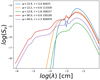 |
Fig. A.1. Examples of AGN templates adopted in the SED fitting with different values of optical depth at 9.7 μm (τ) and the angle between equatorial axis and line of sight (Ψ). |
CIGALE parameters used for the SED fitting.
All Tables
Star formation rate density obtained by integrating the LF best-fit in our eight redshift bins.
All Figures
|
Fig. 1. Number of pointings as a function of observing wavelength in the A3COSMOS database. The wavelength ranges of the ALMA bands are plotted as color-shaded regions. The most populated bands are 6 and 7, with ∼2000 pointings. |
| In the text | |
|
Fig. 2. Archival ALMA observations in the COSMOS field used in this study. Individual pointings are plotted with different colors representing the observed ALMA bands. In the background, the COSMOS field is shown in gray. We show three zoom-in regions representative of possible classes of pointing configurations. Panel a: three overlapping pointings in the same band. Panel b: three concentric pointings in different bands. Panel c: overlapping and concentric pointings in different bands. |
| In the text | |
|
Fig. 3. Examples of SED-fitting results for three different classes of objects. From left to right: Unobscured AGN SED, SED without an AGN contribution, and obscured AGN component. The blue circles and the red triangles represent data points and upper limits, respectively. The best-fit model is plotted as a black solid line. The stellar attenuated and unattenuated, the dust emission, and the AGN emission are respectively reported as a yellow solid line, a blue dashed line, a red solid line, and a green solid line. |
| In the text | |
|
Fig. 4. Distributions of the main physical parameters obtained through SED fitting for the initial and final, reduced, sample. Top-left panel: redshift distribution. Top-right panel: AGN fraction distribution, computed in the 5–40 μm range. Bottom-left panel: logarithm of stellar mass distribution, in units of solar masses. Bottom-right panel: logarithm of the dust luminosity in solar luminosities. |
| In the text | |
|
Fig. 5. Main sequence of galaxies computed in six different redshift bins: 0.5–1.2, 1.2–1.5, 1.5–2.0, 2.0–3.0, 3.0–4.0, 4.0–6.0. Data of the full sample are reported as blue circles, while the red diamonds represent the final sample (Sect. 4.4) used in our analysis. The black solid line and shaded area indicate the main sequence Speagle et al. (2014; computed at the mean values of the redshift bins) and 1σ dispersion. Finally, the black dashed lines represent the 4x MS, indicative of the starburst regime. |
| In the text | |
|
Fig. 6. Ratio between the flux at 1200 μm and other bands against redshift. The gray circles in the background indicate the values for individual sources in each band, while the colored circles refer to the median values in each redshift bin and for each ALMA band, as described in Sect. 4.2. |
| In the text | |
|
Fig. 7. Ratio between the flux at 1200 μm and in other bands against observed wavelength. Each circle is the median value computed as described in Sect. 4.2. The red, brown, gray, and yellow circles are at z < 4.5, while the green circles represent the last redshift bin at z > 4.5. |
| In the text | |
|
Fig. 8. Two overlapping pointings in band 6. The black circle represents the adopted primary beam size (out to a pbcor of 0.2), color-coded by the inferred RMS. Lower RMS values are represented by darker colors and higher values by lighter ones. Outside our primary beam boundary, we set values to the arbitrary high value of 106 μJy. In these types of cases, we adopted the area from the deepest pointing in the overlapping region. |
| In the text | |
|
Fig. 9. Total areal coverage of the 1155 pointings after the cut for a lack of target detection within 1 arcsec. |
| In the text | |
|
Fig. 10. Example of a source with optical identification (photo-z = 0.74) likely distinct from the ALMA galaxy. Left panel (from top to bottom): ALMA, acs-I, UV-j, and IRAC1 images are displayed with ALMA contours overlaid. It can be inferred that the optical/NIR object near the ALMA position is not centered in the ALMA galaxy. Right panel: SED of the same object showing the impossibility of fitting the optical and ALMA millimeter flux simultaneously. |
| In the text | |
|
Fig. 11. A3COSMOS luminosity function (black circles and red boxes). The individual redshift bin MCMC best fit is plotted as pink solid lines and shaded error bands. The redshift ranges are reported in the upper-right corner of each subplot, while the luminosity bins are centered at each 0.25 dex, with a width of 0.5 dex (overlapping bins). The black vertical dashed lines represent the completeness limit of the LIR. The orange dashed, purple dotted, and green dashed lines are the best-fit LFs obtained by Gruppioni et al. (2013, 2020), Magnelli et al. (2013). |
| In the text | |
|
Fig. 12. A3COSMOS (red boxes and black circles) + Herschel (black triangles) luminosity function. The dark-red lines and shaded areas are the best fit obtained by using all the LF points from different z-bins together. The redshift ranges are reported in the upper-right corner of each subplot, while the luminosity bins are centered at each 0.25 dex, with a width of 0.5 dex (overlapping bins). The black vertical dashed lines represent the completeness limit of the LIR. The orange dashed, purple dotted, and green dashed lines are the best-fit LFs obtained by Gruppioni et al. (2013, 2020), Magnelli et al. (2013). |
| In the text | |
|
Fig. 13. Evolutionary trends of Φ* (top panel) and L* (bottom panel) with redshift. The solid dark-red lines and shaded areas show the behaviors of Φ* and L* at all the redshifts, while the pink diamonds are the estimates obtained when fitting each redshift bin individually in the ALMA-only case. Finally, the empty black circles and yellow circles represent estimates for L* and Φ* from Gruppioni et al. (2013, 2020), which we include for comparison. |
| In the text | |
|
Fig. 14. Co-moving SFRD evolution with z. The red diamonds were obtained through the integration of the LF best-fit in each z bin, while the dark-red shaded area was obtained by integrating the evolutionary LF from z= 0.5 to 6. Comparison curves from the literature are reported as gray dash-dotted (pessimistic and optimistic cases; Lagache 2018); dashed (IllustrisTNG), dotted (Béthermin et al. 2017), and black solid lines (Madau & Dickinson 2014). The empty red circles with different symbols represent different IR-millimeter estimates of the SFRD from Gruppioni et al. (2013, 2015, 2020), Magnelli et al. (2013), Rowan-Robinson et al. (2016), Liu et al. (2018), and the orange shaded area is the dust-obscured SFRD by Zavala et al. (2021), from the MORA survey. The SFRD from the UV is plotted as empty blue circles with different markers (Dahlen et al. 2007; Reddy & Steidel 2009; Cucciati et al. 2012; Bouwens et al. 2012, 2015). |
| In the text | |
|
Fig. A.1. Examples of AGN templates adopted in the SED fitting with different values of optical depth at 9.7 μm (τ) and the angle between equatorial axis and line of sight (Ψ). |
| In the text | |
Current usage metrics show cumulative count of Article Views (full-text article views including HTML views, PDF and ePub downloads, according to the available data) and Abstracts Views on Vision4Press platform.
Data correspond to usage on the plateform after 2015. The current usage metrics is available 48-96 hours after online publication and is updated daily on week days.
Initial download of the metrics may take a while.