| Issue |
A&A
Volume 690, October 2024
|
|
|---|---|---|
| Article Number | A84 | |
| Number of page(s) | 10 | |
| Section | Extragalactic astronomy | |
| DOI | https://doi.org/10.1051/0004-6361/202451113 | |
| Published online | 02 October 2024 | |
A3COSMOS: Dust mass function and dust mass density at 0.5 < z < 6
1
Istituto Nazionale di Astrofisica (INAF) – Osservatorio di Astrofisica e Scienza dello Spazio (OAS), Via Gobetti 101, 40129 Bologna, Italy
2
Dipartimento di Fisica e Astronomia (DIFA), Università di Bologna, Via Gobetti 93/2, 40129 Bologna, Italy
3
Université Paris-Saclay, Université Paris Cité, CEA, CNRS, AIM, 91191 Gif-sur-Yvette, France
4
INAF, Osservatorio Astronomico di Brera 28, 20121, Milano, Italy and Via Bianchi 46, 23807 Merate, Italy
5
SISSA, Via Bonomea 265, 34136 Trieste, Italy
6
INAF, Osservatorio Astronomico di Trieste, Via Tiepolo 11, 34131 Trieste, Italy
7
Dipartimento di Fisica e Astronomia “G. Galilei”, Università di Padova, Via Marzolo 8, 35131 Padova, Italy
8
INAF, Istituto di Radioastronomia, Via Piero Gobetti 101, 40129 Bologna, Italy
9
INAF – Osservatorio Astrofisico di Arcetri, Largo E. Fermi 5, 50125 Firenze, Italy
Received:
14
June
2024
Accepted:
11
July
2024
Abstract
Context. Although dust in galaxies represents only a few percent of the total baryonic mass, it plays a crucial role in the physical processes occurring in galaxies. Studying the dust content of galaxies, particularly at high z, is therefore crucial for understanding the link between dust production, obscured star formation, and the build-up of galaxy stellar mass.
Aims. We study the dust properties (mass and temperature) of the largest Atacama Large Millimeter/submillimeter Array (ALMA)-selected sample of star-forming galaxies available from the archive (A3COSMOS), and we derive the dust mass function and dust mass density of galaxies from z = 0.5 − 6.
Methods. We fit the spectral energy distribution (SED) with the CIGALE code to constrain the dust mass and temperature of the A3COSMOS galaxy sample based on the UV-to-near-infrared photometric coverage of each galaxy combined with the ALMA (and Herschel when available) coverage of the Rayleigh-Jeans tail of their dust-continuum emission. We then computed and fit the dust mass function by combining the A3COSMOS and the most recent Herschel samples in order to obtain the best estimate of the integrated dust mass density up to z ∼ 6.
Results. The dust masses in galaxies in A3COSMOS lie between ∼108 and ∼109.5 M⊙. From the SED fitting, we were also able to derive a dust temperature. The distribution of the dust temperature peaks at ∼30 − 35 K. The dust mass function at z = 0.5 − 6 evolves with an increase in M* and a decrease in the number density (Φ*), and it agrees well with literature estimates. The dust mass density decreases smoothly in its evolution from z ∼ 0.5 to z ∼ 6, which is steeper than what is found by models at z ≳ 2.
Key words: surveys / galaxies: evolution / galaxies: high-redshift / galaxies: luminosity function / mass function / galaxies: star formation / submillimeter: galaxies
Corresponding author; This email address is being protected from spambots. You need JavaScript enabled to view it.
© The Authors 2024
 Open Access article, published by EDP Sciences, under the terms of the Creative Commons Attribution License (https://creativecommons.org/licenses/by/4.0), which permits unrestricted use, distribution, and reproduction in any medium, provided the original work is properly cited.
This article is published in open access under the Subscribe to Open model. This email address is being protected from spambots. You need JavaScript enabled to view it. to support open access publication.
1. Introduction
Recent studies have revealed a higher value of the dust-obscured star formation rate density (SFRD) even at high redshift (e.g., Khusanova et al. 2021; Gruppioni et al. 2020; Traina et al. 2024). To understand the origin of this high dust-obscured SFRD, one possibility is to study the dust mass content of the Universe at different cosmic times. This study is crucial for our understanding of the dust-obscured SFRD, and the dust also plays a major role in most astrophysical processes in the evolution of galaxies and active galactic nuclei (AGN) (McKee & Ostriker 2007; Cazaux & Tielens 2002; Hopkins et al. 2012). The reason for and time of the dust emergence is still debated. Deriving the dust mass function (DMF) and the evolution with redshift of the dust mass density (DMD) offers us the opportunity to address this issue via a statistical approach.
In the past years, a number of works have been devoted to the estimation of the dust mass in galaxies and how it scales with other galactic properties in local and distant galaxies (Calura et al. 2017; Herrera-Camus et al. 2018; Pastrav 2020; Casasola et al. 2022), mostly using the Herschel observatory (Dunne et al. 2011; Pozzi et al. 2020; Eales & Ward 2024). However, while these studies were able to trace the DMD from z ∼ 2 − 3 to the present day, they did not probe its evolution at higher redshift because of the limitation of the far-infrared (FIR) in tracing the Rayleigh-Jeans (hereafter R–J) regime of the dust emission (which is needed to derive MD). A sampling of the dust emission at longer wavelengths such as the submillimeter (submm) and millimeter (mm) bands is then crucial to explore the high-z dust content of the Universe. Different studies used submm and mm facilities (e.g., IRAM, ALMA) have investigated the DMD at higher redshift (Magnelli et al. 2019, 2020; Pozzi et al. 2021), and their estimates indicate different contents of dust at high z. Moreover, simulations (Popping et al. 2017; Aoyama et al. 2018; Li et al. 2019; Vijayan et al. 2019) failed to accurately reproduce the observed evolution of the DMD with redshift, and in particular, very few of them were able to reproduce the observed drop at z < 1 (Gioannini et al. 2017; Parente et al. 2023). In this context, deep submm surveys of large galaxy samples and covering a wide redshift range are critical in order to shed light on the evolution of the galaxy dust content across cosmic time.
Although ALMA is characterized by a small field of view, which makes wide-area surveys too demanding observationally, the recent A3COSMOS survey (Liu et al. 2019a,b; Adscheid et al. 2024) circumvents this limitation by collecting and homogeneously analyzing archival ALMA images of dusty star-forming galaxies. This unique survey can also be exploited to characterize the dust mass content and evolution. Even though the A3COSMOS is by construction an inhomogeneous collection of ALMA archival observations, significant effort has been made to statistically turn it from a pointed to a blind-like survey (reducing possible bias sources). This effort has enable a variety of relevant statistical quantities to be derived (i.e., number counts, luminosity function, SFRD; Adscheid et al. 2024; Traina et al. 2024). Continuing to exploit the A3COSMOS database, in this work we characterize the dust properties for the galaxies in the A3COSMOS sample, and estimate the DMF and DMD over a wide (0.5 − 6) redshift range.
The paper is organized as follows. In Section 2 we present the A3COSMOS sample. In Section 3 we describe the methods we used to derive the MD and discuss their differences. In Section 4 we present the results for the DMF and DMD, which we compare to predictions from semi-analytical models and simulations in Section 5. We assume a Chabrier (2003) stellar initial mass function (IMF) throughout and adopt a ΛCDM cosmology with H0 = 70 

 , Ωm = 0.3, and ΩΛ = 0.7.
2. Data sample: A3COSMOS database
The A3COSMOS survey, described by Liu et al. (2019b) and recently updated by Adscheid et al. (2024), consists of the collection of all the archival ALMA observations within the COSMOS field. We used the most recent version of the A3COSMOS combined with the COSMOS2020 photometry (Adscheid et al. 2024), which was already adopted in Traina et al. (2024). Due to the inhomogeneous nature of this database, which arises because each ALMA pointing has its own observing frequency, sensitivity, and particular targeted source, a reduction of all the possible biases affecting the sample is needed. We used the final sample obtained by Traina et al. (2024) (see also Adscheid et al. 2024), in which a blinding process was applied, in order to use this database as a blind survey for statistical purposes. First, to account for possible positional errors between the ALMA target and submm priors from other catalogs, all the pointings without a source in the inner 1’ were removed, together with the area of the inner circle. Clustered galaxies with a redshift similar to that of the target were also removed. Finally, specific conversions to account for different wavelenghts and sensitivities were applied during the calculation of the areal coverage for the so-built A3COSMOS survey. The final sample consists of 189 galaxies, which are considered to be serendipitously detected in the ALMA pointings.
The main integrated galaxy properties (i.e., stellar mass, dust luminosity, and star formation rate) were inferred by Traina et al. (2024), who reported a massive (M⋆ ∼ 1010 − 1012 M⊙), infrared-luminous (LIR, 8 − 1000 ∼ 1011 − 1013 L⊙), and highly star-forming (SFR ∼10 − 1000 M⊙yr−1) population. Based on the SED fitting performed in Traina et al. (2024) (see Fig. 4 in the paper), we also find that ∼30 − 40% of these galaxies probably host an AGN. The AGN contribution to the total SED emission of most of these galaxies is low (i.e., the fraction of the AGN emission to the total IR emission in the 5–40 μm range, fAGN, with a mean value of ∼35%). This sample of star-forming galaxies that were detected at submm and mm with ALMA is particularly well suited for the characterization of the dust properties of SFGs.
3. Dust mass estimation
The IR emission in galaxies originates from dust that is heated either by UV emission from recently formed stars or from the AGN. The dust thermalizes with the radiation and re-emits at longer wavelengths in the IR bands, with a spectrum that can reliably be described by graybody emission (i.e., less efficient than a black body, Bianchi 2013), whose shape is linked to the different dust phases in a galaxy. The warm dust component, close to the heating source (stars or AGN), emits large quantities of luminosity per unit of mass and dominates the FIR emission (where the dust emission peaks). The diffuse dust component in the galaxy, which dominates in mass, is instead heated by a weaker radiation field and therefore has a lower temperatures. This implies a much lower luminosity per unit mass and an emission that peaks at longer wavelengths (submm and mm). The composite contribution of the different dust phases produces the observed peak of the dust emission (λpeak). At λ > λpeak, the graybody emission is in the R–J regime (where cold dust peaks) and can be used to trace the global dust mass in the galaxy. In particular, the R-J emission traces the bulk of the dust reservoir in the galaxy, which is at the mass-weighted temperature, in contrast to the luminosity-weighted temperature, which would be associated with strongly heated dust that emits in the FIR, but is not representative of the total dust mass (see Liang et al. 2019, for a detailed discussion on the different dust temperature definitions). We computed MD relying on the SED fitting or directly from the observed ALMA flux. In the following Sections 3.1 and 3.2, we describe these two possible approaches to deriving MD.
3.1. MD from a spectral energy distribution fitting
The first method for inferring MD of a galaxy is to perform a complete SED fitting of the FIR/mm photometry that traces dust emission. We used the PYTHON SED-fitting tool called Code Investigating GALaxy Emission (CIGALE; Boquien et al. 2019). CIGALE is based on the energy balance between the UV and optical emission by stars and on the re-emission in the IR and mm by the dust, and it allows us to choose among different individual templates for each emission component (e.g., stellar optical/UV emission, cold dust emission, or AGN emission) across a broad parameter space. For the dust emission component, we used the DL14 (Draine et al. 2014) module. Consistently with the dust attenuation component we used, DL14 assumed the diffuse interstellar medium (ISM), heated by the general stellar population in the galaxy, and birth clouds (BCs), heated by newly formed massive stars. The main input parameters are the PAH mass fraction and the minimum radiation field, along with the slope of the dust emission (α) and the illuminated fraction (γ; see Table A.1 in Traina et al. 2024 for the input parameters). The dust mass of the cold component was computed by dividing the dust luminosity (i.e., the luminosity arising from the dust heated by stars) by the dust emissivity, and it was returned as output from the SED fitting. The radiation field (Umin, returned from CIGALE) that heats the dust can be linked to the mass-weighted dust temperature as follows (Aniano et al. 2012):
![Mathematical equation: $$ \begin{aligned} T_{\rm D, CIGALE} = 18 \cdot U_{\rm min}^{1/6} \mathrm{[K]}. \end{aligned} $$](/articles/aa/full_html/2024/10/aa51113-24/aa51113-24-eq4.gif) (1)
(1)
Figure 1 shows the TD, CIGALE distribution, which follows a smoothly rising trend, with a large number of sources having TD, CIGALE ∼ 34K. The median value is ∼31K, which agrees with what is found by Pozzi et al. (2020) from a sample of ∼6000 galaxies observed with Herschel at z ∼ 0 − 2.5.
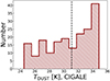 |
Fig. 1. Dust temperature computed using the output radiation field given by the CIGALE SED-fitting analysis (see Eq. (1)). The vertical dashed line indicates the median value for the sample. |
3.2. MD from the R–J flux density
An alternative method for deriving MD consists of using the flux at a certain wavelength in the R–J part of the SED. Following the optically thin approximation, MD can be computed as follows:
 (2)
(2)
where Bνobs(Tobs) is the blackbody Planck function computed at the observed frame mass-weighted temperature (Tobs = TD/(1 + z)), Sνobs is the flux density at the observed frequency νobs, with νrest = (1 + z)νobs, κνo is the photon cross-section to mass ratio of dust at the rest-frame ν0, and β is the dust emissivity spectral index (see e.g., Magnelli et al. 2020). The approximation of being in the optically thin regime has already been assumed in several works in the literature (see e.g., Magnelli et al. 2020; Pozzi et al. 2021) and has been proved to be valid when the bulk of the galaxy population has a cold dust component (as in our case) and when the observed flux is in the R–J regime (Scoville et al. 2014, 2016, 2017). In our analysis, we adopted a value of κ = 0.0469 m2kg−1, derived for a wavelength of 850 μm (Draine et al. 2014), to be consistent with the CIGALE estimates. For the spectral index of the dust emissivity, β, typical values are between 1.5 and 2.0 (with a good agreement between empirical measurements and theoretical predictions Dunne & Eales 2001; Clements et al. 2010; Draine 2011). We used β = 1.8, as suggested by Scoville et al. (2014) based on the findings of the Planck Collaboration XXV (2011).
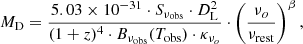
After κν0 and β were fixed, the main parameters that affect MD are the flux at the observed frequency νobs and the rest-frame mass-weighted temperature TD. Several works suggested (or used) a dust temperature in a range between ∼15K and ∼40K (see e.g., Dunne et al. 2011; Dale et al. 2012; Magnelli et al. 2014; Pozzi et al. 2020, 2021). As can be inferred from Eq. (2), lower dust temperatures correspond to higher dust masses and vice versa, leading to uncertainties between 25% and 50% for MD with a different TD assumption (Magnelli et al. 2020). We chose to use two values of the rest-frame temperature, namely TD = 25K and TD = 35K, which encompass the range of possible values for the mass-weighted TD. This is supported by observations and models (see e.g., Magnelli et al. 2014; Sommovigo et al. 2020). Magnelli et al. (2014) indeed found that only a small fraction of galaxies with a high sSFR have a TD > 35K. To estimate MD from the observed flux, we chose to use the ALMA flux at the longest available wavelength (SALMA, long). In our sample, the longest observed ALMA band always corresponds to rest-frame values above λ ∼ 200μm, enabling us to to probe the R–J tail for every galaxy in our sample (see Figure 2).
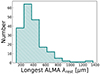 |
Fig. 2. Rest-frame wavelength corresponding to the longest observed ALMA band fluxes for each galaxy in the sample. |
In Figure 3, we show the distributions for MD computed with the two different methods (SED fit or single MBB) and with two different temperatures of the MBB (25K and 35K). The median values of the 25K and 35K dust masses are  M⊙ (hereafter MD, 25K) and
  M⊙ (hereafter MD, 35K). In this case, the 25K MD is higher by a factor ∼2 than that of 35K. Moreover, as expected from the TD distribution of the CIGALE SEDs (see Fig. 1), the MD, 35K and MD, CIGALE agree very well, with a difference of only ∼0.04 dex in their median values.
 |
Fig. 3. Dust mass distribution as inferred using our three different approaches, i.e., the longest observed ALMA fluxes and assuming a single MBB with a dust temperature of 25K (cyan histogram) and 35K (magenta histogram). The dark red distribution corresponds to the dust masses given as an output of the CIGALE SED fitting. |
In the rest of our analysis, we decided to derive the DMF and DMD using these three different dust mass estimates, that is, MD, cigale, MD, 25K, and MD, 35K. MD, cigale can be considered as our fiducial estimate because it is independent of the assumption made on the dust temperature and of the reference wavelength of the monochromatic flux. MD, 35K should provide a very consistent measurement, but has the advantage compared to MD, cigale that it solely rely on the observed mm flux without the need for the UV-to-IR energy balance assumption made in CIGALE. Finally, while MD, 25K seems to be disfavored in Fig. 3, we decided to keep it because the 25K assumption is commonly made in the literature (Magnelli et al. 2020; Pozzi et al. 2021).
4. Dust mass function and dust mass density
4.1. VMAX method and the dust mass function
In order to derive the DMF, we applied the Schmidt (1970) maximum comoving volume (VMAX) method. Based on the data, this method allowed us to derive the observed DMF without making any assumption relative to its shape. The areal coverage as a function of the flux has already been derived by Traina et al. (2024) for the A3COSMOS survey at a reference observed wavelength of 1200 μm. This relation between cumulative area and limiting fluxes was used to associate an accessible area above a certain flux with each source.
We derived the DMF in eight redshift bins from z ∼ 0.5 to z ∼ 6 and into dust mass bins with a width of 0.5 dex from log( to log(
 . For each source in a z-MD bin, the contribution to the DMF was obtained as follows. At first, we shifted the best-fit SED in redshift and K-corrected it from the lower to the upper boundary of the corresponding redshift bin and computed its flux at 1200 μm. Then, we used this flux to infer the corresponding areal coverage at each dz (i.e., the redshift step used to shift the SED of each source) by interpolating the areal coverage versus flux density curve derived in Traina et al. (2024). We finally combined the effective area obtained in this way with the element of the volume at each redshift step and obtained a comoving volume over which a given source is accessible,
 (3)
(3)
where Vzmax and Vzmin are the sum of the subvolume in each dz shell up to the upper and lower limits of the bin, respectively. In particular, Vzmax can either be the volume at the upper bound of each dz bin or the maximum volume that can be reached by considering the S/N limit of the survey (i.e., corresponding to the z at which the area would be zero). Finally, we corrected VMAX by taking into account the completeness and spuriousness corrections derived by Liu et al. (2019b), and we obtained the Φ(M, z) by summing each 1/VMAX in a certain luminosity-redshift bin. The completeness threshold was computed by rescaling all the observed 1200 μm fluxes of each SED to the faintest observed 1200 μm flux density in this redshift bin and then taking the highest MD of these SEDs. This latter value represents the MD below which our sample is not entirely complete. We derived the DMFs using either the dust mass inferred from CIGALE or from the ALMA observed flux at the longest wavelength available and assuming TD = 25K, TD = 35K. In each case, we divided the sample into eight similarly populated redshift bins (0.5–1.0, 1.0–1.5, 1.5–2.0, 2.0–2.5, 2.5–3.0, 3.0–3.5, 3.5–4.5, and 4.5–6.0). Fig. 4 shows the three dust mass functions derived with the different assumptions (i.e., DMFcigale, DMF25K, and DMF35K), and the data points of our fiducial DMF are reported in Table 1.
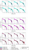 |
Fig. 4. Dust mass function derived using the VMAX method for dust masses of the galaxies computed assuming TD = 25K (cyan squares and black circles with errors, computed following Gehrels 1986, upper panel), TD = 35K (magenta squares and black circles with errors, central panel) and using the dust mass from CIGALE (red squares and black circles with errors, lower panel). The best fit, computed using the A3COSMOS data points, is displayed as a solid red line, with shaded error bands of the same color. For this fit, MD*, ΦD*, and α were free to vary. For comparison, different estimates from the literature are reported. The light blue circles and squares are the values obtained by Pozzi et al. (2020), and the dashed cyan lines correspond to the best fit. The dashed gray curves are from Dunne et al. (2003). The blue circle show the estimate by Magnelli et al. (2019), and the dotted line shows the ALPINE dust mass function by Pozzi et al. (2021), assuming TD = 25K. |
Dust mass function inferred from the A3COSMOS database.
We compared our DMF data points with the few estimates that are available in similar redshift ranges from the literature. In particular, at 0.5 < z < 2.5, we compared the A3COSMOS DMFs with the results by Pozzi et al. (2020). It is first important to underline the main differences between the two samples. The Herschel data sample is much larger than the A3COSMOS sample (∼6000 and ∼190 galaxies, respectively), which leads to lower uncertainties on the estimated DMFs. Moreover, the Herschel sample traces a wider range of dust masses at the faint (due to a better sensitivity) and at the bright ends (larger comoving volume). In the redshift and luminosity range in common, in the A3COSMOS and the Herschel results, we find a weak agreement with the DMF25K and a much better consistency when using the 35K dust masses, as well as the CIGALEMD. This agreement could be explained by the method used by Pozzi et al. (2020) to derive TD, which considered the dust temperature as a function of the redshift and the specific star formation rate (Magnelli et al. 2014), which led to TD > 25K (i.e., lower MD values) that increased with redshift to ∼35 − 40 K at z ∼ 2. At higher redshift, very few works have investigated the DMF. In Figure 4 and 5, we report the Dunne et al. (2003) DMF at 1 < z < 5 (obtained from a SCUBA sample of dusty galaxies), the point by Magnelli et al. (2019) at 3.1 < z < 4.6, derived using the IRAM/GISMO 2mm Survey in the COSMOS field, and the ALPINE DMF at z ∼ 4.5 (Pozzi et al. 2021). Within the large uncertainties of our data points, the three DMF estimates agree with the best fit by Dunne et al. (2003). While DMF35K and DMFCIGALE agree very well with the data point by Magnelli et al. (2019) at z ∼ 3.5, the DMF25K is weakly consistent within the errors. Finally, as expected, our DMF25 agrees very well with the ALPINE DMF estimate, which was derived assuming TD = 25K.
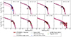 |
Fig. 5. Dust mass functions derived using the VMAX method for dust masses of the galaxies obtained via SED fitting (red boxes and black circles with errors, computed following Gehrels 1986). The evolutive best fit of the CIGALE + Herschel is displayed as a solid red line, with shaded error bands of the same color, and the individual A3COSMOS fit is shown as the shaded pink area. The errors on the evolutive best fit are computed by bootstrapping on the dust masses of the sources. For comparison, different estimates from the literature are reported. The light blue circles and squares show the values obtained by Pozzi et al. (2020), and the dashed cyan lines correspond to the best-fit. The dashed gray curves are from Dunne et al. (2003). The blue circle shows the estimate by Magnelli et al. (2019), and the dashed line is the ALPINE dust mass function by Pozzi et al. (2021). |
4.2. Markov chain Monte Carlo fitting analysis
To obtain the best-fit parameters characterizing the DMF at different redshifts, we performed a Markov chain Monte Carlo (MCMC) fitting analysis and modeled the DMF with a Schechter function (that has been found to be a better parametrization than the modified-Schechter, often used to fit the IR-LF, Pozzi et al. 2020),
![Mathematical equation: $$ \begin{aligned} \Phi (M_{\rm D})\mathrm{dlog}M_{\rm D} = \Phi ^*\left(\frac{M_{\rm D}}{M^*_{\rm D}}\right)^{\alpha } \mathrm{exp}\left[-\frac{M_{\rm D}}{M^*_{\rm D}}\right]\mathrm{dlog}M_{\rm D}, \end{aligned} $$](/articles/aa/full_html/2024/10/aa51113-24/aa51113-24-eq61.gif) (4)
(4)
where α is the slope of the faint end, and MD* and Φ* represent the dust mass and normalization at the knee, respectively. Pozzi et al. (2020) also reported an evolutionary trend with redshift for these parameters, expressed as
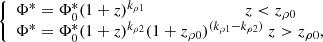 (5)
(5)
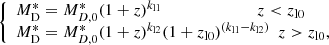 (6)
(6)
where Φ0* and MD, 0* are the normalization and characteristic dust mass at z = 0 and kρ1, kρ2, kl1, and kl2 are the exponents for values lower and greater than zρ0 and zl0 for Φ and MD, respectively. We thus performed an MCMC fit using simultaneously each point of the DMF associated with a redshift corresponding to the median redshift value of the underlying galaxy population in the bin.
We carried out the MCMC analysis using the PYTHON package emcee (Foreman-Mackey et al. 2013), using a set of 50 walkers and 10 000 steps to explore the parameter space, discarding the first 1000 sampled draws of each walker (burn-in). The log-likelihood was built in the following form:
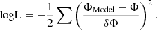 (7)
(7)
With this procedure, we obtained a first best fit of the three DMFs by running the MCMC and leaving the Schechter parameters (i.e, α, Φ*, and M*) free to vary (see Fig. 4). For DMF25K, MD* is significantly higher than reported by Pozzi et al. (2020), and the best fit has a very different shape. The DMF35K is instead more consistent with the Pozzi et al. (2020) estimate and the best fit also agrees better, even though MD* is still higher. By fitting the DMF using only the A3COSMOS data, we cannot constrain all parameters of the Schechter function robustly.
To improve the quality of our fit, as done by Traina et al. (2024) to derive the LF best fit, we exploited the Herschel data derived by Pozzi et al. (2020) to fit a combined A3COSMOS + Herschel DMF. The greater statistic of the Herschel data at 0 < z < 2.5 allowed us to combine the accuracy of the DMF by Pozzi et al. (2020) at lower-medium redshifts, with the capability of ALMA to explore the dust content of galaxies in the high-z Universe. With these combined datasets, we were able to constrain the shape of the DMF better and to derive more reliable best-fit parameters. The Herschel DMF was derived by assuming that the dust temperature is a function of z and of the sSFR, as reported in Magnelli et al. (2014). This means that the galaxies in that sample do not have a fixed temperature, so that it is not possible to coherently combine these estimates of the DMF with our DMF25K or DMF35K. For this reason, we decided to combine the Pozzi et al. (2020) DMF with the CIGALE DMF because it does not assume a fixed temperature and is also more consistent with the Pozzi et al. (2020) data. We ran the MCMC with α fixed to the values found by Pozzi et al. (2020) (i.e., α = 1.48) using flat prior distributions for the two free parameters (Φ* and M*), with log(Φ0*) between −2.5 and −2 and log(MD, 0*) between 6 and 7.5. The results of this DMF fit are shown in Figure 5 and are summarized in Table 2. We consider this best fit our fiducial DMF. As a comparison, we also overplot the best fit obtained considering the A3COSMOS DMF data points in each redshift bin separately. This fit shows larger errors due to the lower number of data, and the Schechter parameters also differ from what we obtained with the evolutive fit. The typical dust mass at each redshift bin (i.e., MD*) from our fiducial best fit increases almost constantly by ∼1 dex from z ∼ 0.5 to z ∼ 6. This means that because for LIR*, massive galaxies are typically more dust rich at higher redshifts than their local counterparts. Similarly, the density Φ* decreases steeply toward higher redshifts (by ∼2 dex). Comparing these values with those from the individual fit (see Figure 6), we note that without the combination with the Herschel data, the typical MD* is nearly constant, while the density (Φ*) decreases at z > 3.
Best-fit parameters at the knee of the DMF inferred by combining the A3COSMOS dataset with the Herschel data points.
 |
Fig. 6. Evolution with redshift of MD* and Φ* obtained by fitting the A3COSMOS and Herschel DMFs (dashed red lines and shaded areas), compared to the same parameters derived by fitting the A3COSMOS CIGALE DMF in each redshift bin separately (pink circles). |
4.3. Dust mass density
By integrating the DMF best fit (at 4 < log(MD/M⊙) < 11) in each redshift bin, we can measure the amount of dust per unit of comoving volume and obtain the DMD. Figure 7 shows the DMD obtained by integrating the combined A3COSMOS CIGALE and Herschel DMF best fit. We report the values of the DMD in Table 3. To allow the comparison of the results by Magnelli et al. (2020) and Pozzi et al. (2021) with ours, we rescaled their DMDs from T = 25K to T = 35K (i.e., MD, 35K = 0.54 × MD, 25K; see Section 3). The DMD follows the shape of the Pozzi et al. (2020) DMD, with a smoother decrease from z = 1 to higher redshifts. Our results agree excellently with the estimates by Ménard & Fukugita (2012), which were obtained for MgII absorbers. We are also consistent with the DMD from Driver et al. (2018), who studied galaxies from the GAMA, G10-COSMOS, and 3D-HST surveys, between z ∼ 1 and z ∼ 2. Our results are consistent with those of Magnelli et al. (2020) at z ∼ 1.5 − 3. The DMD by Péroux & Howk (2020) is instead significantly lower between z ∼ 1.5 and z ∼ 4. The reason for the discrepancy with our result may be ascribed to a possible selection bias in the estimate by Péroux & Howk (2020) (also mentioned in their paper) toward dust-poor galaxies. Their results are indeed based on a sample of optically selected quasars, for which they derived the DMD by combining the gas mass density and the dust-to-gas ratio. At z ∼ 4.5, our results are fully consistent with the results obtained from the rest-frame FIR-selected galaxies in the ALPINE ALMA survey (Pozzi et al. 2021). Comparing our results with the recent estimates by Eales & Ward (2024), obtained using Herschel-ATLAS, we find a good agreement at z ∼ 1.5, while our DMD is lower at 2 < z < 3 and slightly higher at 3 < z < 5.
 |
Fig. 7. DMD evolution with redshift, derived by integrating the CIGALE + Herschel dust mass function in each redshift bin (shaded red area). The pink circles with errors represent the DMD obtained by fitting the DMF individually at each redshift bin. The red plus marker shows the values by Dunne et al. (2003), the green triangles show the estimates by Vlahakis et al. (2005), the red triangles show the DMD points by Dunne et al. (2011), the blue triangles indicate the estimate by Ménard & Fukugita (2012), the red crosses show the data points by Driver et al. (2018); the red circles show the data by Beeston et al. (2018), the estimate by Magnelli et al. (2019) is shown as a filled green circle, the empty green circles are the points by Péroux & Howk (2020), the estimates by Pozzi et al. (2021) are shown as blue and red circles; the DMDs from Magnelli et al. (2020) are displayed as filled blue circles; the black points show the DMD estimates by Eales & Ward (2024), and finally, the light blue shaded area represents the estimate of the DMD by Pozzi et al. (2020). For a self-consistent comparison, we rescaled the data by Magnelli et al. (2020) and Pozzi et al. (2021) to TD = 35K. |
DMDy obtained by integrating the DMF best fit in our eight redshift bins for the CIGALE A3COSMOS + Herschel fit.
5. Discussion
In this section, we compare our results with the predictions for the DMF and DMD from models in the literature. In particular, we considered the semi-analytical model by Parente et al. (2023) for comparison to the DMF and the predictions by Gioannini et al. (2017), Popping et al. (2017), Aoyama et al. (2018), Li et al. (2019), Vijayan et al. (2019), Triani et al. (2020), Parente et al. (2023), and Yates et al. (2024) to compare with the DMD.
Although different in the details implementation, the dust models in the aforementioned works are conceptually similar. They all include (i) dust production by stellar sources (SNe and AGB stars), (ii) dust evolution in the ISM, in particular, accretion of gas-phase metals onto preexisting grains, and destruction of grains in hostile environments (e.g., SN shocks and the hot phase), and (iii) astration of grains, that is, grains returning into newly formed stars. All these processes play a role in determining the amount of dust present in galaxies. Specifically, the evolution of dust within the ISM turns out to be very important. Simulations indeed indicate that the bulk of the dust mass observed today originates from grain accretion within the ISM, while stellar production only contributes a small fraction (≲10%) to the overall dust budget (e.g., Vijayan et al. 2019; Parente et al. 2023).
The DMD predicted by the aforementioned model is shown in Fig. 8. There is a great dispersion that spans about one order of magnitude at all redshifts. There is also no agreement in terms of shape. In some of the models (e.g., Triani et al. 2020; Popping et al. 2017), a ρdust increases with cosmic time, while some others (e.g. Gioannini et al. 2017; Aoyama et al. 2018; Li et al. 2019; Parente et al. 2023) predict a clear drop from z ≃ 1 − 2 to z = 0, which is more in line with observations. In general, none of the models is able to match both the shape and normalization of the observed ρdust.
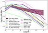 |
Fig. 8. Comparison between our DMD (derived using the CIGALE dust masses) and the predictions from simulations. The solid purple line shows the DMD by Gioannini et al. (2017), and the dashed purple line represents the prediction by Popping et al. (2017). The dotted magenta line shows the prediction by Aoyama et al. (2018), the dotted cyan line shows the DMD predicted by Vijayan et al. (2019), the dotted light green curve shows the results by Triani et al. (2020), the dotted red line shows the prediction by Li et al. (2019), and the solid pink line shows the DMD from Yates et al. (2024). The dashed gray, light blue, yellow, green, and blue lines are the DMDs estimated using the models by Parente et al. (2023) with different prescriptions. |
The different performances of the various models in predicting the cosmic dust abundance originate in distinct underlying reasons that are challenging to determine. First, while the theoretical frameworks of these models are conceptually similar, their practical numerical implementation can vary significantly. Second, a major contributing factor could be that the dust model is implemented in addition to different galaxy evolution models, each incorporating subgrid recipes for processes (e.g., star formation and chemical enrichment) that are crucial for the production and evolution of dust mass. It is not trivial to analyze these disparities, and it goes beyond the scope of the current work. We instead adopted an alternative approach with the aim to quantify the influence of specific dust-related mechanisms, namely, stellar production, ISM accretion, and SN-driven destruction, on the overall dust budget. To do this, we standardized the galaxy evolution framework to accentuate the impacts of the targeted processes. Specifically, we conducted multiple simulations using the Parente et al. (2023) model1 to explore potential ways to increase the dust mass at the redshifts investigated here. The conducted simulations are listed below.
-
cond_enhancedx5: The dust condensation efficiency was enhanced by a factor of 5 to mimic a larger dust production by stellar sources (both AGBs and SNe).
-
acc_time_reducedx3: The ISM grain accretion timescale was reduced by a factor of 3 to mimic a more efficient accretion in molecular clouds.
-
acc_time_reducedx10: The same as before, but the timescale was reduced by a factor of 10.
-
no_SNe_destruction: Grains destruction in SN shocks was switched off.
In Fig. 8 we present the DMD results from these experiments. Switching off grain destruction by SNe increases the overall dust abundance only marginally compared to the fiducial run. This occurs because the metals generated by the SNe-driven destruction rapidly recombine into dust grains through the highly efficient accretion process. Similarly, increasing the AGBs and SNe production of grains has a minor effect on the DMD, raising it by a factor of ≃1.4 at z ≳ 1. Conversely, increasing the efficiency of grain accretion has a stronger impact on the DMD, boosting it by a factor of ≳2 compared to the fiducial model, which brings it closer to our A3COSMOS estimate. Nevertheless, both the acc_time_reducedx3 and acc_time_reducedx10 simulations overestimate the DMD at z ≲ 0.5.
At higher redshifts, in the range probed by our data (z > 1.5 − 2), any of the reported models is able to reproduce the normalization and the shape of the observed DMD. In particular, the slope of the predicted DMDs is typically steeper than what is found observationally at z > 1.5. This lack of dust in high-z galaxies in the models could be due to a lack of the most highly star-forming IR-bright galaxies in the simulations, as found by Gruppioni et al. (2015), Katsianis et al. (2017). Based on our analysis performed by modifying the model by Parente et al. (2023), we argue that the currently implemented dust physics alone does not cause the observed discrepancies. Other sources of a difference might arise from the different physical processes incorporated in the models. This is further supported by the large variation among the other models, which are based on different galaxy evolution simulations. Building on this clue, we might speculate that one way of improving the models would then be to make a cross-comparison with a variety of different observables. For example, it would be interesting to investigate how the dust-richest high-z galaxies appear in terms of SFR, size, and morphology. This study would enable us to improve the galaxy evolution model in several aspects, and hopefully achieve a better match with observations.
Since the A3COSMOS DMD is derived from the integration of the observed DMF, it is also interesting to compare the latter for the aforementioned SAM-based experiments, as shown in Fig. 9. As previously mentioned, modifying the stellar production and switching off the SNe-driven grain destruction has very little impact on the predicted DMF. Conversely, enhancing the accretion efficiency brings the SAM predictions closer to the observed DMF, particularly at z ≳ 2 in the accx10 run. In our experiments, this is the only way to generate objects with dust masses similar to the observed masses (≃109 M⊙). We additionally note a discrepancy between the simulated DMFs and the extrapolated Schechter fit at Mdust ≲ 108 M⊙, where direct observations are unavailable.
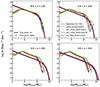 |
Fig. 9. Comparison between the DMF derived in this work (solid black line with shaded area and red points) and the predictions by Parente et al. (2023), with different prescriptions. |
We conclude this section with two caveats regarding our numerical experiments. The first caveat concerns the underlying galaxy evolution framework of the model. Specifically, the SAM by Parente et al. (2023) has been noted to exhibit a lack of highly star-forming galaxies at z ≳ 1 (Traina, in prep.). These galaxies also host substantial amounts of dust, the same dust that is missing in Fig. 9. Second, while increasing accretion alleviates discrepancies with observations, we caution that it may affect the relation between the dust-gas ratio and ISM metallicity (Parente et al. 2022). This topic is beyond the scope of this study.
6. Summary and conclusions
We have investigated the properties of the dust mass budget in high-redshift galaxies. To this end, we studied a sample of 189 ALMA-selected star-forming galaxies in a wide redshift range (0.5 < z < 6), drawn from the A3COSMOS database. By performing an SED-fitting analysis, we measured the dust content of each galaxy (i.e., dust mass and temperature), and we used these estimates to derive the DMF and the DMD. We summarize our results below.
-
The A3COSMOS star-forming galaxies are dust rich, with SED-based dust masses between 108 and 109 M⊙. Most of them show a TD ∼ 30 − 35K.
-
RJ-based dust masses agree well with masses based on the SED fit when the assumed dust temperature is roughly consistent with those inferred from our SED fit (∼35K), while the dust mass estimate with TD = 25 is ∼54% higher.
-
The DMF inferred from the MD derived from the SED fit agrees well with those derived by Pozzi et al. (2020) in the mass and redshift range in common between these two studies.
-
Combining the Herschel and ALMA DMFs, we inferred for the first time the evolution of the DMFs over a wide range of redshifts (0.5 < z < 6). The characteristic density (Φ*) and mass (MD*) of the DMFs evolve with a decreasing (∼2 dex) and increasing (∼1dex) trend with redshift, respectively.
-
Integrating the DMFs, we found that the DMD evolves with a smoothly decreasing trend from z ∼ 0.75 to z ∼ 5.25. It shows no drastic drop toward higher redshifts.
-
None of the models available in literature is able to match both the shape and the normalization of the observed DMD at 0.5 < z < 5. Through dedicated numerical experiments, we find that the grain accretion in the ISM is the most effective dust-related process for increasing the dust content of galaxies.
This is based on the L-GALAXIES SAM (Henriques et al. 2020). It is noteworthy that this model is able to reproduce the general trend of redshift evolution of the DMD within the uncertainties (see Fig. 10 of Parente et al. 2023).
Acknowledgments
We would like to thank the anonymous referee for the positive and constructive report. I.D. acknowledges funding by the European Union – NextGenerationEU, RRF M4C2 1.1, PRIN 2022JZJBHM: “AGN-sCAN: zooming-in on the AGN-galaxy connection since the cosmic noon” – CUP C53D23001120006
References
- Adscheid, S., Magnelli, B., Liu, D., et al. 2024, A&A, 685, A1 [NASA ADS] [CrossRef] [EDP Sciences] [Google Scholar]
- Aniano, G., Draine, B. T., Calzetti, D., et al. 2012, ApJ, 756, 138 [Google Scholar]
- Aoyama, S., Hou, K.-C., Hirashita, H., Nagamine, K., & Shimizu, I. 2018, MNRAS, 478, 4905 [NASA ADS] [CrossRef] [Google Scholar]
- Beeston, R. A., Wright, A. H., Maddox, S., et al. 2018, MNRAS, 479, 1077 [NASA ADS] [Google Scholar]
- Bianchi, S. 2013, A&A, 552, A89 [NASA ADS] [CrossRef] [EDP Sciences] [Google Scholar]
- Boquien, M., Burgarella, D., Roehlly, Y., et al. 2019, A&A, 622, A103 [NASA ADS] [CrossRef] [EDP Sciences] [Google Scholar]
- Calura, F., Pozzi, F., Cresci, G., et al. 2017, MNRAS, 465, 54 [Google Scholar]
- Casasola, V., Bianchi, S., Magrini, L., et al. 2022, A&A, 668, A130 [NASA ADS] [CrossRef] [EDP Sciences] [Google Scholar]
- Cazaux, S., & Tielens, A. G. G. M. 2002, ApJ, 575, L29 [NASA ADS] [CrossRef] [Google Scholar]
- Chabrier, G. 2003, PASP, 115, 763 [Google Scholar]
- Clements, D. L., Dunne, L., & Eales, S. 2010, MNRAS, 403, 274 [NASA ADS] [CrossRef] [Google Scholar]
- Dale, D. A., Aniano, G., Engelbracht, C. W., et al. 2012, ApJ, 745, 95 [NASA ADS] [CrossRef] [Google Scholar]
- Draine, B. T. 2011, Physics of the Interstellar and Intergalactic Medium [Google Scholar]
- Draine, B. T., Aniano, G., Krause, O., et al. 2014, ApJ, 780, 172 [Google Scholar]
- Driver, S. P., Andrews, S. K., da Cunha, E., et al. 2018, MNRAS, 475, 2891 [Google Scholar]
- Dunne, L., & Eales, S. A. 2001, MNRAS, 327, 697 [Google Scholar]
- Dunne, L., Eales, S. A., & Edmunds, M. G. 2003, MNRAS, 341, 589 [NASA ADS] [CrossRef] [Google Scholar]
- Dunne, L., Gomez, H. L., da Cunha, E., et al. 2011, MNRAS, 417, 1510 [NASA ADS] [CrossRef] [Google Scholar]
- Eales, S., & Ward, B. 2024, MNRAS, 529, 1130 [NASA ADS] [CrossRef] [Google Scholar]
- Foreman-Mackey, D., Hogg, D. W., Lang, D., & Goodman, J. 2013, PASP, 125, 306 [Google Scholar]
- Gehrels, N. 1986, ApJ, 303, 336 [Google Scholar]
- Gioannini, L., Matteucci, F., & Calura, F. 2017, MNRAS, 471, 4615 [NASA ADS] [CrossRef] [Google Scholar]
- Gruppioni, C., Calura, F., Pozzi, F., et al. 2015, MNRAS, 451, 3419 [Google Scholar]
- Gruppioni, C., Béthermin, M., Loiacono, F., et al. 2020, A&A, 643, A8 [NASA ADS] [CrossRef] [EDP Sciences] [Google Scholar]
- Henriques, B. M. B., Yates, R. M., Fu, J., et al. 2020, MNRAS, 491, 5795 [NASA ADS] [CrossRef] [Google Scholar]
- Herrera-Camus, R., Sturm, E., Graciá-Carpio, J., et al. 2018, ApJ, 861, 95 [Google Scholar]
- Hopkins, P. F., Quataert, E., & Murray, N. 2012, MNRAS, 421, 3522 [Google Scholar]
- Katsianis, A., Blanc, G., Lagos, C. P., et al. 2017, MNRAS, 472, 919 [NASA ADS] [CrossRef] [Google Scholar]
- Khusanova, Y., Bethermin, M., Le Fèvre, O., et al. 2021, A&A, 649, A152 [NASA ADS] [CrossRef] [EDP Sciences] [Google Scholar]
- Li, Q., Narayanan, D., & Davé, R. 2019, MNRAS, 490, 1425 [CrossRef] [Google Scholar]
- Liang, L., Feldmann, R., Kereš, D., et al. 2019, MNRAS, 489, 1397 [NASA ADS] [CrossRef] [Google Scholar]
- Liu, D., Schinnerer, E., & Groves, B. 2019a, Astrophysics Source Code Library [record ascl: 1910.003] [Google Scholar]
- Liu, D., Schinnerer, E., Groves, B., et al. 2019b, ApJ, 887, 235 [Google Scholar]
- Magnelli, B., Lutz, D., Saintonge, A., et al. 2014, A&A, 561, A86 [NASA ADS] [CrossRef] [EDP Sciences] [Google Scholar]
- Magnelli, B., Karim, A., Staguhn, J., et al. 2019, ApJ, 877, 45 [NASA ADS] [CrossRef] [Google Scholar]
- Magnelli, B., Boogaard, L., Decarli, R., et al. 2020, ApJ, 892, 66 [NASA ADS] [CrossRef] [Google Scholar]
- McKee, C. F., & Ostriker, E. C. 2007, ARA&A, 45, 565 [Google Scholar]
- Ménard, B., & Fukugita, M. 2012, ApJ, 754, 116 [Google Scholar]
- Parente, M., Ragone-Figueroa, C., Granato, G. L., et al. 2022, MNRAS, 515, 2053 [NASA ADS] [CrossRef] [Google Scholar]
- Parente, M., Ragone-Figueroa, C., Granato, G. L., & Lapi, A. 2023, MNRAS, 521, 6105 [NASA ADS] [CrossRef] [Google Scholar]
- Pastrav, B. A. 2020, MNRAS, 493, 3580 [NASA ADS] [CrossRef] [Google Scholar]
- Péroux, C., & Howk, J. C. 2020, ARA&A, 58, 363 [CrossRef] [Google Scholar]
- Planck Collaboration XXV. 2011, A&A, 536, A25 [NASA ADS] [CrossRef] [EDP Sciences] [Google Scholar]
- Popping, G., Somerville, R. S., & Galametz, M. 2017, MNRAS, 471, 3152 [NASA ADS] [CrossRef] [Google Scholar]
- Pozzi, F., Calura, F., Zamorani, G., et al. 2020, MNRAS, 491, 5073 [NASA ADS] [CrossRef] [Google Scholar]
- Pozzi, F., Calura, F., Fudamoto, Y., et al. 2021, A&A, 653, A84 [NASA ADS] [CrossRef] [EDP Sciences] [Google Scholar]
- Schmidt, M. 1970, ApJ, 162, 371 [NASA ADS] [CrossRef] [Google Scholar]
- Scoville, N., Aussel, H., Sheth, K., et al. 2014, ApJ, 783, 84 [CrossRef] [Google Scholar]
- Scoville, N., Sheth, K., Aussel, H., et al. 2016, ApJ, 820, 83 [Google Scholar]
- Scoville, N., Lee, N., Vanden Bout, P., et al. 2017, ApJ, 837, 150 [Google Scholar]
- Sommovigo, L., Ferrara, A., Pallottini, A., et al. 2020, MNRAS, 497, 956 [NASA ADS] [CrossRef] [Google Scholar]
- Traina, A., Gruppioni, C., Delvecchio, I., et al. 2024, A&A, 681, A118 [NASA ADS] [CrossRef] [EDP Sciences] [Google Scholar]
- Triani, D. P., Sinha, M., Croton, D. J., Pacifici, C., & Dwek, E. 2020, MNRAS, 493, 2490 [NASA ADS] [CrossRef] [Google Scholar]
- Vijayan, A. P., Clay, S. J., Thomas, P. A., et al. 2019, MNRAS, 489, 4072 [NASA ADS] [CrossRef] [Google Scholar]
- Vlahakis, C., Dunne, L., & Eales, S. 2005, MNRAS, 364, 1253 [NASA ADS] [CrossRef] [Google Scholar]
- Yates, R. M., Hendriks, D., Vijayan, A. P., et al. 2024, MNRAS, 527, 6292 [Google Scholar]
All Tables
Best-fit parameters at the knee of the DMF inferred by combining the A3COSMOS dataset with the Herschel data points.
DMDy obtained by integrating the DMF best fit in our eight redshift bins for the CIGALE A3COSMOS + Herschel fit.
All Figures
|
Fig. 1. Dust temperature computed using the output radiation field given by the CIGALE SED-fitting analysis (see Eq. (1)). The vertical dashed line indicates the median value for the sample. |
| In the text | |
|
Fig. 2. Rest-frame wavelength corresponding to the longest observed ALMA band fluxes for each galaxy in the sample. |
| In the text | |
|
Fig. 3. Dust mass distribution as inferred using our three different approaches, i.e., the longest observed ALMA fluxes and assuming a single MBB with a dust temperature of 25K (cyan histogram) and 35K (magenta histogram). The dark red distribution corresponds to the dust masses given as an output of the CIGALE SED fitting. |
| In the text | |
|
Fig. 4. Dust mass function derived using the VMAX method for dust masses of the galaxies computed assuming TD = 25K (cyan squares and black circles with errors, computed following Gehrels 1986, upper panel), TD = 35K (magenta squares and black circles with errors, central panel) and using the dust mass from CIGALE (red squares and black circles with errors, lower panel). The best fit, computed using the A3COSMOS data points, is displayed as a solid red line, with shaded error bands of the same color. For this fit, MD*, ΦD*, and α were free to vary. For comparison, different estimates from the literature are reported. The light blue circles and squares are the values obtained by Pozzi et al. (2020), and the dashed cyan lines correspond to the best fit. The dashed gray curves are from Dunne et al. (2003). The blue circle show the estimate by Magnelli et al. (2019), and the dotted line shows the ALPINE dust mass function by Pozzi et al. (2021), assuming TD = 25K. |
| In the text | |
|
Fig. 5. Dust mass functions derived using the VMAX method for dust masses of the galaxies obtained via SED fitting (red boxes and black circles with errors, computed following Gehrels 1986). The evolutive best fit of the CIGALE + Herschel is displayed as a solid red line, with shaded error bands of the same color, and the individual A3COSMOS fit is shown as the shaded pink area. The errors on the evolutive best fit are computed by bootstrapping on the dust masses of the sources. For comparison, different estimates from the literature are reported. The light blue circles and squares show the values obtained by Pozzi et al. (2020), and the dashed cyan lines correspond to the best-fit. The dashed gray curves are from Dunne et al. (2003). The blue circle shows the estimate by Magnelli et al. (2019), and the dashed line is the ALPINE dust mass function by Pozzi et al. (2021). |
| In the text | |
|
Fig. 6. Evolution with redshift of MD* and Φ* obtained by fitting the A3COSMOS and Herschel DMFs (dashed red lines and shaded areas), compared to the same parameters derived by fitting the A3COSMOS CIGALE DMF in each redshift bin separately (pink circles). |
| In the text | |
|
Fig. 7. DMD evolution with redshift, derived by integrating the CIGALE + Herschel dust mass function in each redshift bin (shaded red area). The pink circles with errors represent the DMD obtained by fitting the DMF individually at each redshift bin. The red plus marker shows the values by Dunne et al. (2003), the green triangles show the estimates by Vlahakis et al. (2005), the red triangles show the DMD points by Dunne et al. (2011), the blue triangles indicate the estimate by Ménard & Fukugita (2012), the red crosses show the data points by Driver et al. (2018); the red circles show the data by Beeston et al. (2018), the estimate by Magnelli et al. (2019) is shown as a filled green circle, the empty green circles are the points by Péroux & Howk (2020), the estimates by Pozzi et al. (2021) are shown as blue and red circles; the DMDs from Magnelli et al. (2020) are displayed as filled blue circles; the black points show the DMD estimates by Eales & Ward (2024), and finally, the light blue shaded area represents the estimate of the DMD by Pozzi et al. (2020). For a self-consistent comparison, we rescaled the data by Magnelli et al. (2020) and Pozzi et al. (2021) to TD = 35K. |
| In the text | |
|
Fig. 8. Comparison between our DMD (derived using the CIGALE dust masses) and the predictions from simulations. The solid purple line shows the DMD by Gioannini et al. (2017), and the dashed purple line represents the prediction by Popping et al. (2017). The dotted magenta line shows the prediction by Aoyama et al. (2018), the dotted cyan line shows the DMD predicted by Vijayan et al. (2019), the dotted light green curve shows the results by Triani et al. (2020), the dotted red line shows the prediction by Li et al. (2019), and the solid pink line shows the DMD from Yates et al. (2024). The dashed gray, light blue, yellow, green, and blue lines are the DMDs estimated using the models by Parente et al. (2023) with different prescriptions. |
| In the text | |
|
Fig. 9. Comparison between the DMF derived in this work (solid black line with shaded area and red points) and the predictions by Parente et al. (2023), with different prescriptions. |
| In the text | |
Current usage metrics show cumulative count of Article Views (full-text article views including HTML views, PDF and ePub downloads, according to the available data) and Abstracts Views on Vision4Press platform.
Data correspond to usage on the plateform after 2015. The current usage metrics is available 48-96 hours after online publication and is updated daily on week days.
Initial download of the metrics may take a while.