| Issue |
A&A
Volume 645, January 2021
|
|
|---|---|---|
| Article Number | A110 | |
| Number of page(s) | 20 | |
| Section | Interstellar and circumstellar matter | |
| DOI | https://doi.org/10.1051/0004-6361/202038608 | |
| Published online | 22 January 2021 | |
A population of hypercompact H II regions identified from young H II regions★
1
Max Planck Institute for Radio Astronomy,
Auf dem Hügel 69,
53121
Bonn,
Germany
e-mail: ayyang@mpifr-bonn.mpg.de
2
Centre for Astrophysics and Planetary Science, University of Kent,
Canterbury,
CT2 7NH,
UK
3
Centre for Astrophysics Research, School of Physics Astronomy & Mathematics, University of Hertfordshire,
College Lane, Hatfield, AL10 9AB,
UK
4
CAS Key Laboratory of FAST, National Astronomical Observatories, Chinese Academy of Sciences, Beijing 100012, PR China
5
University of Chinese Academy of Sciences,
19A Yuquan Road,
Shijingshan District,
Beijing 100049,
PR China
6
Kavli Institute for Astronomy and Astrophysics, Peking University,
Beijing 100871,
PR China
Received:
8
June
2020
Accepted:
13
November
2020
Context. The derived physical parameters for young H II regions are normally determined assuming the emission region to be optically thin. However, this assumption is unlikely to hold for young H II regions such as hyper-compact H II (HC H II) and ultra-compact H II (UC H II) regions and leads to underestimation of their properties. This can be overcome by fitting the SEDs over a wide range of radio frequencies.
Aims. The two primary goals of this study are (1) to determine the physical properties of young H II regions from radio SEDs in the search for potential HC H II regions, and (2) to use these physical properties to investigate their evolution.
Methods. We used the Karl G. Jansky Very Large Array (VLA) to observe the X-band and K-band with angular resolutions of ~1.7′′ and ~0.7′′, respectively, toward 114 H II regions with rising-spectra (α1.4 GHz5 GHz>0). We complement our observations with VLA archival data and construct SEDs in the range of 1−26 GHz and model them assuming an ionization-bounded H II region with uniform density.
Results. Our sample has a mean electron density of ne = 1.6 × 104 cm−3, diameter diam = 0.14 pc, and emission measure EM = 1.9 × 10⁷ pc cm−6. We identify 16 HC H II region candidates and 8 intermediate objects between the classes of HC H II and UC H II regions. The ne, diam, and EM change, as expected, but the Lyman continuum flux is relatively constant over time. We find that about 67% of Lyman-continuum photons are absorbed by dust within these H II regions and the dust absorption fraction tends to be more significant for more compact and younger H II regions.
Conclusions. Young H II regions are commonly located in dusty clumps; HC H II regions and intermediate objects are often associated with various masers, outflows, broad radio recombination lines, and extended green objects, and the accretion at the two stages tends to be quickly reduced or halted.
Key words: H II regions / evolution / radio continuum: stars / stars: massive / stars: formation
Full Tables 1, 3 and 5 are only available at the CDS via anonymous ftp to cdsarc.u-strasbg.fr (130.79.128.5) or via http://cdsarc.u-strasbg.fr/viz-bin/cat/J/A+A/645/A110
© A. Y. Yang et al. 2021
 Open Access article, published by EDP Sciences, under the terms of the Creative Commons Attribution License (https://creativecommons.org/licenses/by/4.0), which permits unrestricted use, distribution, and reproduction in any medium, provided the original work is properly cited.
Open Access funding provided by Max Planck Society.
1 Introduction
One key question regarding massive star formation in the youngest H II region relates to how accretion proceeds against the outward pressure therein (e.g., Keto & Wood 2006), as massive stars reach the main sequence while still accreting (e.g., Zinnecker & Yorke 2007; Motte et al. 2018). However, many details of the earliest stages of H II regions are unclear. Simple analytic models suggest that the H II region can be created by either the inner, ionized part of the inflowing material (Keto 2002, 2003) or the ionized photoevaporative outflow (Hollenbach et al. 1994) fed by accretion (Keto 2007). The onset time for the development of a H II region is found to be early in the McKee & Tan (2003) and Peters et al. (2010) turbulent core and ionization feedback models, but the models of Hosokawa & Omukai (2009) and Hosokawa et al. (2010) for a bloated protostar suggest that this onset is later on. After the birth of H II regions, the subsequent expansion has been modeled as uniform spherical bubbles (Spitzer 1978), or asymmetrical flows into outflow-driven cavities (Peters et al. 2010), and the expansion rates predicted by different models could also be different (e.g., Bisbas et al. 2015). Detailed observations toward the youngest H II regions are crucial to investigate their initial development and constrain theoretical models (Thompson et al. 2015, 2016).
The two youngest H II region stages are commonly known as hyper-compact H II (HC H II) and ultra-compact H II (UC H II) regions (e.g., Kurtz 2005). The youngest is the HC H II region with a typical physical size (diam) of diam ≲ 0.05 pc, an electron density (ne) of ne ≳105 cm−3, an emission measure (EM) of EM ≳ 108 pc cm−6, and a radio recombination line (RRL) with a line width of ΔV ≳ 40 km s−1 (Kurtz et al. 2000; Sewilo et al. 2004; Hoare et al. 2007; Murphy et al. 2010). The UC H II region is thought to be the next evolutionary stage after the HC H II region, with diam ≲ 0.1 pc, ne ≳104 cm−3, EM ≳ 107 pc cm−6, and ΔV ~ 25−30 km s−1 (e.g., Wood & Churchwell 1989; Afflerbach et al. 1996; Hoare et al. 2007). The defining characteristics of these two stages (i.e., diam, ne, and EM) are somewhat arbitrary, as the evolution from HC H II regions to UC H II regions is thought to be continuous (e.g., Garay & Lizano 1999; Yang et al. 2019). Compared to the hitherto discovered ~600 UC H II regions (Urquhart et al. 2007, 2009a, 2013; Lumsden et al. 2013; Cesaroni et al. 2015; Kalcheva et al. 2018; Djordjevic et al. 2019), only 16 HC H II regions have been identified in previous studies (summarized by Yang et al. 2019 and references therein). It is not yet clear at what stage and how an HC H II region evolves into an UC H II region. Given the fact that the observed sizes of young H II regions are found to vary with observing frequency (Panagia & Felli 1975; Avalos et al. 2006), it has been suggested that the classical quantitative criteria for identifying HC H II regions should be modified in order to consider the variations (Yang et al. 2019), which could lead to a better understanding of the intermediate object between an HC H II region and an UC H II region. However, to understand the relation between the two classes, and eventually to understand the early stages of newly formed massive stars, reliable properties toward a large sample of HC H II regions and UC H II regions are needed to be determined.
Although young H II regions around massive stars are heavily obscured by a thick cocoon of molecular gas, they can nevertheless be studied at radio wavelengths thanks to the ability of radio radiation to penetrate the dense molecular gas. Therefore, most studies of young H II regions are based on radio continuum observations (e.g., Wood & Churchwell 1989; Kurtz et al. 1994; van der Tak & Menten 2005; Gibb & Hoare 2007). The radio continuum spectrum of an H II region with spectral index α (Sν ∝ να) varies from + 2 (optically thick) at low frequency to − 0.1 (optically thin) at high frequency. The turnover frequency between the optically thick and thin regimes for thermal bremsstrahlung is essentially a linear function of the electron density (Mezger & Henderson 1967). A younger H II region with higher density will remain optically thick at higher frequencies. For instance, UC H II regions have a typical turnover frequency of νt ~ 5 GHz, while HC H II regions have νt = 10 to 100 GHz (e.g., Beltrán et al. 2007; Hoare et al. 2007; Keto et al. 2008; Zhang et al. 2014). Therefore, young H II regions with spectra still rising in a higher frequency are potentially young and dense, which might correspond to an early stage of UC H II region or a stage connecting UC H II and HC H II regions.
The physical properties of young H II regions have been measured in several previous studies (e.g., Wood & Churchwell 1989; Murphy et al. 2010; Urquhart et al. 2013; Kalcheva et al. 2018; Medina et al. 2019), either by a targeted multi-band observation on small samples of UC H II regions (e.g., Murphy et al. 2010) or using single-band surveys assuming that the gas is optically thin to free-free emission (e.g., Urquhart et al. 2013; Kalcheva et al. 2018). The assumption that H II regions are optically thin would give unreliable physical properties if the H II region is actually optically thick at the observed frequency. Therefore, multi-band data taken over a large range of frequencies are crucial in order to reliably determine the physical properties of young H II regions.
In this work, we present the results of multi-band observations with the Karl G. Jansky Very Large Array1 (VLA) in X-band (8–12 GHz) and K-band (18–26 GHz) of a sample of 114 young H II regions. These sources were selected from a sample of H II regions with rising spectra between 1.4 GHz and 5 GHz, that is,  (Yang et al. 2019). Together with archival VLA data at 1.4 and 5 GHz (see Sect. 2.1 for details), we measure the spectral energy distribution (SED) between 1 and 26 GHz for each source in the sample, which covers both optically thick and thin portions of their radio spectra. We model every SED to find the best estimates for the physical properties.
This paper is organized as follows: Sect. 2 describes the details of the sample, observation, and data reduction. Section 3 presents and discusses the observational results, the modeled SEDs, and the radio properties of the sources and their distributions. In Sect. 4, we discuss HC H II region candidates, plus a small sample of objects considered to be in an intermediate phase between HC H II and UC H II regions. In Sect. 5 we discuss the relations and distribution of all of the UC H II and HC H II regions. We present a summary of this work and highlight our conclusions in Sect. 6.
2 Observation
2.1 Sample selection
In Yang et al. (2019), we constructed a parent sample of 534 objects with rising radio spectral indexes between 1.4 and 5 GHz using three JVLA surveys, THOR (The HI, OH, Recombination line survey of the Milky Way, Bihr et al. 2016; Beuther et al. 2016), MAGPIS (The Multi-Array Galactic Plane Imaging Survey, White et al. 2005; Helfand et al. 2006), and CORNISH (Coordinated Radio “N” Infrared Survey for High-mass star formation, Hoare et al. 2012; Purcell et al. 2013). From an analysis of the combined radio, infrared, and submillimeter emission properties (Yang et al. 2019), we identified 120 young H II regions from the parent sample. This sample not only recovers previously known HC H II regions, but also includes broad RRL objects with line widths of ΔV > 40 km s−1 and a number ofUC H II regions with positive spectra (Yang et al. 2019). We observed 114 young H II regions in X- and K-band data taken with the VLA. We use the data from archives and the literature for the four sources in the initial sample that have not been observed in the project, marked with a star in Tables 1 and 7. The final sample includes 118 young H II regions.
The flux densities and angular diameters of the 118 observed sources are given in Table 1. The 1.4 and 5 GHz flux densities are taken from Yang et al. (2019) and references therein. The distances and bolometric luminosities are mainly drawn from the results reported in Urquhart et al. (2018)2, which includes 105 objects of the sample. For the remaining 13 sources with no measurements in Urquhart et al. (2018), their distances and bolometric luminosities are taken from three studies, namely Cesaroni et al. (2015), Urquhart et al. (2013), and Kalcheva et al. (2018). The kinematic distances were computed by fitting the radial velocity of each source to the Galactic rotation curve. The kinematic distances near/far ambiguity (KDA) for sources within the solar circle was resolved by CO emission line data and H I absorption (e.g., Urquhart et al. 2013; Cesaroni et al. 2015; Yang et al. 2016; Kalcheva et al. 2018) or using a combination of H I analysis, maser parallax, and spectroscopic measurements (Urquhart et al. 2018). The bolometric luminosity of the sample was taken from the same reference as the distance and was determined by integrating the SED from near-infrared to submillimeter wavelengths (e.g., König et al. 2017).
Observed 114 rising spectra H II regions.
Summary of VLA observation parameters.
2.2 Observations and data reduction
Observations of 114 young H II regions were carried out using the VLA in C configuration. Instrument parameters used are shown in Table 2. The observations were made at X-band (8–12 GHz) and K-band (18–26 GHz), split into two subbands with 30 channels at X-band, and four subbands with 60 channels at K-band, each channel with a bandwidth of 128 MHz, full stokes. The synthesized beams in C configuration at X-band and K-band are ~ 1.8′′ and ~ 0.7′′, and the FWHM primary beams sizes are ~ 4.2′ and ~ 2′, respectively. The typical on-source time for each target is about one minute and the total observation time is 4.5 h. The phase calibrators (J1832-1035, J1851-0035, and J1922+1530) were observed every half hour at X-band and every 12 min at K-band to correct the amplitude and phase of the interferometer data by atmospheric and instrumental effects. The pointing corrections at the high-frequency K-band were determined by observing the nearby phase calibrators in interferometric pointing mode. The absolute flux density scale at X-band and K-band was calibrated by comparing the observations of the standard flux density scale calibrator J1331+305 (3C286) with its models provided by the NRAO.
Standard calibration and data reduction were performed using the Common Astronomy Software Applications package (CASA, McMullin et al. 2007). Raw VLA data were calibrated and reduced by running the CASA pipeline. We discarded the first 3 s of data of every scan for calibrators to exclude the antenna settling time. Flux and phase calibrator data were carefully examined to ensure high-quality data. A calibration table was produced and applied to all targeted data. Each target was inspected by eye to flag bad data such as phase scatters, errant amplitudes, system-temperature spikes, which resulted in a mean on-source integration time of ~50 s for each source.
Images were constructed using the default Briggs robust parameter of zero, which provides a good trade-off between the low thermal noise of natural weighting and the high resolution of uniform weighting. Because of short on-source time (~50 s), we adopted to widest possible frequency ranges for each image to do the clean task in CASA. In order to measure flux density at different frequencies, we produced multi-band images at X-band and K-band. At X-band, three images were produced at central frequencies of 9 GHz (8–10 GHz), 10 GHz (8–12 GHz), and 11 GHz (10–12 GHz). Also, at K-band, three images were produced at central frequencies of 20 GHz (18–22 GHz), 22 GHz (18–26 GHz), and 24 GHz(22–26 GHz). The final beam size of images at the central frequency of X-band, namely 10 GHz, and at the central frequency of K-band, that is 22 GHz, are ~2.1′′× 1.4′′ and ~ 0.7′′ × 0.6′′, respectively. Sources with θ <1.8′′ (X-band) and θ <0.8′′ (K-band) are considered to be unresolved. Sources with angular size θ >1.8′′ (X-band) and θ >0.8′′ (K-band) are considered to be resolved and the deconvolved sizes are given in Table 3.
3 Results and analysis
3.1 Observational results
In Fig. 1, we present images of three sources that show the typical variation in emission structure observed in our sample. Thecontour levels shown in these images were determined using a dynamic range power-law fitting scheme to meaningfully represent both high and low dynamic range images (e.g., Thompson et al. 2006; Urquhart et al. 2009a; Yang et al. 2018). This has been slightly altered from the scheme described by Thompson et al. (2006) and can be described as the following relationship D = 5 × Ni + 5, where D is the dynamic range of the map (defined as the ratio between the peak brightness and the 1σ RMS noise), N is the number of contour lines, and ‘i’ is the contour power-law index. Here, the minimum power-law index was one, which resulted in linearly spaced contours starting at 5σ and increasing in steps of 5σ. The starting contour level we adopted for each target is variable, ranging from 5σ to 7σ according to the RMS level of each image. The RMS noise level (σ) of each image was determined using the standard deviation (STDEV = 1.4826 × MADFM), where MADFM is the median absolute deviation from the median (MADFM = median  , where X is one element in the data set), in order to reduce the effects of outliers on noise measurement (e.g., Purcell et al. 2013). The short on-source integration time of the target observation (~ 50 s) could lead to a rather high RMS level on the observed field for some sources located in complex star formation regions.
The compact sources in the sample are directly fitted by 2D Gaussian models using the imfit task in CASA (see upper panels of Fig. 1). The resolved UC H II regions are classified into a variety of morphologies ranging from spherical to irregular (e.g. Wood & Churchwell 1989; Urquhart et al. 2007, 2009a, 2013; Purcell et al. 2013). The properties of the extended sources (see the middle row of Fig. 1) and UC H II regions located within a cluster (see the lower row of Fig. 1) are determined from the flux enclosed within a polygon fitted around the emission profile of the source; this is determined by the noise level for an extended source manually fitted around the emission for a cluster source, which follows the same strategy used in the construction of the CORNISH survey catalog (Purcell et al. 2013). The observational results of the extended sources or cluster sources in the sample such as flux density (defined as the difference between the aperture summed flux and background flux density divided by the beam-area) and angular diameter (defined as intensity-weighted diameter), as well as their uncertainties, can be measured by aperture photometry (for details of the aperture photometry method that we used see Sect. 5.3.2 of Purcell et al. 2013).
Analysis of the poor-quality X-band and K-band data for seven young H II regions (marked by † in Table 1) revealed that their images are too confused to obtain reliable results and so these have been excluded. We also add five sources identified as UC H II regions in CORNISH by Purcell et al. (2013) that are located within our fields and have rising spectra between C-band and X band in this work. Thus, the final observed sample consists of 112 H II regions. In Table 3, we give the observational results and the derived properties for all of these sources.
In Table4, we provide a statistical summary of the observed and derived properties for each source at both the X-band and K-band. We estimate the uncertainties on the flux density and angular size at both frequencies to typically be ~10% by considering the calibration errors and errors of the measurement method (e.g., Murphy et al. 2010; Sánchez-Monge et al. 2013). In Fig. 2, we show the distributions of the derived parameters. The distributions of integrated flux Sint and peak flux density Speak in the left and middle panels of Fig. 2 are similar at X-band and K-band, which suggests that the majority of sources are optically thin between these frequencies. The X-band shows a slightly higher peak value of Sint and Speak than K-band, some of which may be due to the majority of sources having a turnover frequency below X-band and the fluxes start to decrease afterwards following the power-law of Sν ∝ ν−0.1 at the optically thin regime of an H II region. Some sources may be due to the larger beam at X-band collecting more flux. The X-band has a larger field of view and is more sensitive to larger angular scales than K-band, which is why a larger proportion of the sources detected at X-band are more extended in the right panel of Fig. 2.
Observational results of 112 young H II regions at X-band (8–12 GHz) and K-band (18–26 GHz).
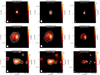 |
Fig. 1 Example images of three radio sources at C-band (left-column), X-band (middle-column), and K-band (right-column). The position of the H II region is marked with a plus. Upper, middle, and lower rows: maps for the compact H II region G032.7441−00.0755, the extendedH ii region G035.4669+00.1394, and the H II region G043.1665+00.0106 located in a cluster (see Sect. 3.1), respectively. C-band images are from the CORNISH survey. The white contour levels of each image are equally spaced by 5σ and start at a level of 5σ. The green outline shown in the lower row shows the polygon that was manually drawn around the H II region located in acluster. The image size and beam size are shown in the upper-middle and lower-left of each image. The C-band, X-band, and K-band images for the whole sample are available in electronic form at the Zenodo via https://doi.org/10.5281/zenodo.4293684. |
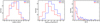 |
Fig. 2 Distributions of observation results such as integrated flux density Sint, peak flux density Speak, and angular size θ, of 116 young H II regions at X-band (blue solid line) and K-band (red solid line). The bin sizes are 0.5 dex, 0.5 dex, and 1′′ for Sint, Speak, and θ, respectively. |
Summary of observational results and the derived physical parameters for 116 young H II regions.
3.2 Radio properties from the SED models
The physical characteristics of H II regions (e.g., EM, ne, Lyman-continuum flux NLy) can be estimated by the observed angular sizes and flux densities at a given frequency, assuming that the continuum emission comes from a homogeneous, optically thin ionized gas (e.g., Urquhart et al. 2013; Kalcheva et al. 2018). However, one should keep in mind that the physical properties of young H II regions might be underestimated or overestimated by using a single frequency observation for two reasons: (i) the young H II region might be optically thick at the observed frequency (e.g., Cesaroni et al. 2015); and (ii) the apparent angular size depends on the observing frequency (e.g., Panagia & Felli 1975; Avalos et al. 2006; Yang et al. 2019). Therefore, to determine the properties of young H II regions, it is essential to know their spectral energy distribution (SED) over a wide frequency range that covers both optically thick and thin emission (e.g., Murphy et al. 2010).
We use our multi-wavelength VLA data to construct SEDs for the free-free emission in order to measure the radio properties of our sample of young H II regions. We model each SED for an ionization-bounded H II region using the standard uniform electron density model given by Mezger & Henderson (1967). In this standard model, the integrated flux density at a given frequency ν is given by 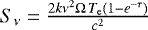 using the Rayleigh Jeans approximation, where Ω is the solid angle related to the physical diameter diam and distance d of each source. The optical depth τ of free–free radiation can also be represented as a function of frequency (Mezger & Henderson 1967; Dyson & Williams 1997),
 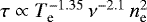 diam, where we assume an electron temperature Te = 104 K (Dyson & Williams 1997). Therefore, the radio SED of an H II region from the standard model is expected to have a rising spectrum at low frequencies sν ∝ ν+2 (τ ≫ 1) and a flat spectrum at high frequencies sν ∝ ν−0.1 (τ ≪ 1). Based on the distances d in Table 1 and the observed fluxes sν in Table 2, the SED model of each source has two free parameters: the electron density ne and the physical diameter diam. The best estimate for the two parameters can be obtained by fitting the radio-frequency continuum spectrum of each source. The uncertainties on flux measurements at these points are taken into account in the fitting process. For compact and spherical H II regions in the sample, the derived density ne and diameter diam from SED fitting represent averaged properties over the ionized gas that are responsible for the free–free emission between 1 and 26 GHz. For the H II regions with non-spherical geometry, this spherical morphology model might introduce additional uncertainty into the determination of the geometry-dependent parameters such as the electron density and diameter. Ideally, the calculation should consider the three-dimensional structure of the volume responsible for the radio emission; however, we do not know the internal structure and any model of the source geometry would introduce additional unknown parameters. Moreover, the morphologies of the nonspherical H II regions are variable between X-band and K-band as shown in Fig. 1. To avoid the complication when calculating the geometry-dependent parameters, the peak physical properties averaged over the beam rather than the entire source are commonly used for these nonspherical and irregular H II regions in previous studies (e.g., Wood & Churchwell 1989; Kurtz et al. 1994). In this work, the uniform spherical model is sufficient to match the SEDs of the nonspherical H II regions, and the SED of each source takes into account the multi-band radio emission of the entire source. Therefore, the fitted ne and diam represent averaged properties over the entire emission gas at multi-bands and can be usedto shed light on the physical condition of these nonspherical H II regions as a whole.
Figure 3 shows examples of the fitted SEDs for a compact source G032.7441−0.076 and an extended source G035.4669+00.1394. Owing to the lack of short baseline spacings, the K-band flux measurements have been excluded from the SED fitting of the extended sources in the sample. Including the four sourceswith data from archives and references (see Sect. 4 and Table 8), the SEDs and best-fitting models of all 116 H II regions are presented in electronic form at the Zenodo3. The EM of each H II region is then calculated using  diam. Considering a mean error of ~10% both in the flux density at each frequency and the distance measurement, this gives typical errors of ~20% in ne, ~10% in diam, and ~40% in EM. The typical errors that we adopted refer to the uncertainty on measurements, as in previous studies (e.g., Sánchez-Monge et al. 2013; Kalcheva et al. 2018), and would be larger if the uncertainty on the assumptions in the model were considered.
The fitted parameters from radio SEDs are given in Table 5 along with the physical parameters derived from the analysis presented in the following section. In panels a–c of Fig. 4, we presentthe distributions of the fitted parameters. The physical sizes peak at 0.02 pc in panel a, and 57% of the sources (66/116) have physical diameters of less than 0.1 pc, as shown in the subplot of that panel. This is consistentwith the majority of these being classified as UC H II regions or smaller. There are 9 sources with diam < 0.01 pc and the mean diameter is diam = 0.006 pc, corresponding to ~1000 AU. This physical scale implies that the sample could have coincidences with radio jets and jet candidates from massive young stellar objects (MYSOs; Purser et al. 2016).
Figure 4b shows the distribution of ne, which peaks at 104 cm−3. About 60% (70/116) of the sources have high densities with ne > 104 cm−3. The 70 high-density H II regions are compact with a mean diameter of diam = 0.06 pc, implying that there might exist small-scale and high-density objects in the sample such as HC H II regions (Kurtz 2005) and MYSO jets (Purser et al. 2016).
Figure 4c shows the distribution of EM, which peaks at 107 pc cm−6, and most sources have EM between 3.2 × 10⁶ pc cm−6 and 1.0 × 10⁸ pc cm−6. There are two groups in the distribution of EM: one with EM < 108 pc cm−6 and the other with EM > 108 pc cm−6, which indicates that there are sources in the sample connected to the very early stages of H II regions.
The median values of diameter (diam = 0.08 pc), electron density (ne = 1.3 × 104 cm−3), and EM (EM = 1.9 × 10⁷ pc cm−6) of our sample are consistent with typical values for UC H II regions. About 10% of the sources have ne > 105 cm−3, 36% of the sample show diam < 0.05 pc, and 17% of them have EM > 108 pc cm−6, which fulfill the standard quantitative criteria of HC H II regions. We discuss the potential HC H II regions in the sample in Sect. 4.
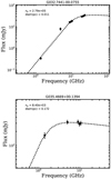 |
Fig. 3 Radio SED fitting to flux density points for example compact and extended sources. Upper panel: SED fitting to flux density points between 1 and 26 GHz for the compact example G032.7441−00.0755 (upper row of Fig. 1). Lower panel: SED fitting to flux density points between 1 and 11 GHz for extended example G035.4669+00.1394 (middle row of Fig. 1) by excluding K-band flux measurements. The best-fitting results for the electron density ne and physical linear diameter diam are shown in the upper-left corner of each plot. The best-fitting SEDs for the whole sample are available in electronic form at the Zenodo via https://doi.org/10.5281/zenodo. 4293684. |
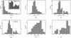 |
Fig. 4 Distributions of the derived physical properties of 116 young H II regions. Panels a–c: distributions of the physical linear diameter diam (a), the electron density ne (b), and the EM (c). The bin sizesare 0.05 pc, 0.25 dex, and 0.25 dex for diam, ne, and EM, respectively. Panels d–f: distributions of the turnover frequency νt (d), the Lyman continuum flux NLy (e), and the dust absorption fraction fd (f). The bin sizesare 0.1, 0.1, and 0.5 dex for νt, fd, and NLy, respectively. |
3.3 Derived physical characteristics
3.3.1 Turnover frequency νt
As a dividing line between the optically thin and thick regimes of the radio spectrum of H II region, the turnover frequency νt is defined as the frequency where τ = 1 (Kurtz 2005). The flux density of H II region peaks at ν > νt, and decreases as the square of frequency at ν < νt. Using the formula provided in Mezger & Henderson (1967) for a homogeneous H II region, the optical depth can be expressed as a function of observing frequency ν, electron temperature Te, which is assumed to be 104 K, and emission measure EM:
![\begin{equation*}\tau = 0.082\;{\times}\;{\left[\frac{T_{\textrm{e}}}\textrm{K}\right]}^{-1.35}\;{\times}\;\,{\left[\frac{\nu}\textrm{GHz}\right]} ^{-2.1}\;{\times}\;\,\left[\frac{\textrm{EM}}{\textrm{pc\,cm}^{-6}}\right], \end{equation*}](/articles/aa/full_html/2021/01/aa38608-20/aa38608-20-eq7.png) (1)
(1)
Setting τ = 1, the turnoverfrequency can be expressed as (Kurtz 2005):
![\begin{equation*}\left[\frac{\nu_{\textrm{t}}}\textrm{GHz}\right] = 0.082\;{\times}\;{\left[\frac{T_{\textrm{e}}}\textrm{K}\right]}^{-1.35}\;{\times}\; \left[\frac{n_{\textrm{e}}^{2}\;{\times}\; \textrm{diam}}{\textrm{cm}^{-3}\,pc}\right]^{0.476}\,\\ \end{equation*}](/articles/aa/full_html/2021/01/aa38608-20/aa38608-20-eq8.png) (2)
(2)
The typical error for the νt is 30% by considering the typical 20% error in density estimation and 10% in diameter measurements. Panel d of Fig. 4 presents the distribution of the turnover frequency νt for this sample of young H II regions (i.e., young UC H II regions), which peaks at νt ~ 2 GHz and has a mean value of νt ~ 3.3 GHz. Both of the peak and mean turnover frequencies of this sample of young H II regions are lower than the expected value of ~ 5 GHz of UC H II regions in Kurtz (2005) with typical ne ~ 3 × 104 cm−3 and diam ~ 0.1 pc. This lower turnover frequency found in the sample may be due to a large fraction of detected emission from the optically thin low-density region surrounded by a H II region, as suggested in Steggles (2016, 2017). Alternatively, many of these H II regions are simply optically thin.
Figure 4d indicates two populations of H II regions: one with νt < 5 GHz and the other with νt > 5 GHz, which are referred to as optically thin and optically thick H II regions in this work, respectively. The optically thick H II regions are found to have higher density, higher emission measure, and smaller physical linear size compared to optically thin H II regions, as shown in Table 6.
3.3.2 Lyman continuum flux
For an optically thin H II region in the photoionization equilibrium, the Lyman continuum ionizing flux NLy emitted by the embedded massive star can be calculated from the radio continuum flux and heliocentric distance to the source (Sánchez-Monge et al. 2013), as
![\begin{equation*}\left[\frac{N_{\textrm{Ly}}}{\mathrm{s}^{-1}}\right]\,=\,8.9\;{\times}\;10^{40}~\left[\frac{S_{\nu}}{\mathrm{Jy}}\right] \left[ \frac{\nu}{\textrm{GHz}} \right]^{0.1} \left[\frac{T_{\mathrm{e}}}{10^4\mathrm{K}}\right]^{-0.45} \left[\frac{d}{\mathrm{pc}}\right]^2, \end{equation*}](/articles/aa/full_html/2021/01/aa38608-20/aa38608-20-eq9.png) (3)
(3)
where Sν is the integrated flux density at frequency ν, Te is electron temperature assumed to be 104 K, and d is the distance to the source. For each source in thesample, we use the Sν measured in the optically thin part of the radio SED to calculate the Lyman continuum flux. The distance for each source is taken from the literature (as discussed in Sect. 2.1). The typical error of the derived Lyman continuum flux is ~ 40% considering the error in both kinematic distance and the integrated flux measurement (e.g., Urquhart et al. 2013).
The distribution of the derived Lyman continuum flux is shown in Fig. 4e, which peaks at 1048 s−1 and ranges from 1045.4 to 1049.9 s−1. The corresponding spectral types of the zero-age main sequence (ZAMS) stars are between B0 and O4 listed in Table 5, assuming that a single star is responsible for the ionization and there is no dust in the ionization-bounded H II region (e.g., Garay et al. 1993; Wood & Churchwell 1989). The derived spectral type of the ZAMS star would be earlier or later (e.g., Wood & Churchwell 1989), if multiple stars are responsible for the ionization or if there is dust absorption within the H II region (e.g., Garay et al. 1993). For instance, the presence of dust may lower the flux by a factor of two or more as the dust absorption fraction ranges from ~50% to ~90% for UC H II regions (e.g., Wood & Churchwell 1989; Garay et al. 1993; Kurtz et al. 1994), but if the emission was from a cluster then the spectral type would be typically earlier by a subclass or two (Wood & Churchwell 1989; Urquhart et al. 2013). The effects of cluster and dust on determining the spectral type are probably comparable and counterbalance each other. Therefore, the values we estimated are reliable within a few subclasses.
3.3.3 Dust within H II regions
Previous studies found that a significant fraction of the Lyman continuum photons are absorbed by the dust within H II regions (Garay et al. 1993; Wood & Churchwell 1989; Kim & Koo 2001). By assuming that a single star is responsible for the observed luminosity and the observed Lyman continuum flux of an H II region, the fraction of UV photons absorbed by dust within H II regions is defined as 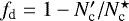 (e.g., Wood & Churchwell 1989), where
  is the number of observed ionizing photons and
  the predicted Lyman continuum photons derived from spectral type based on the total infrared luminosity. As discussed in previous studies (e.g., Garay et al. 1993; Wood & Churchwell 1989), fd should be taken as an upper limit as it is very likely to be overestimated if the expected Lyman continuum photons are excited by clusters of young stars rather than by a single star. For instance, at a given total luminosity, the spectral type estimated assuming a cluster that provides the entire infrared luminosity is typically two or three subclasses later than the spectral type estimated assuming a single star (Wood & Churchwell 1989), and thus leads to a lower expected Lyman continuum flux
  than derived assuming a single star. The observed
  would be dominated by the earliest spectral type in the clusters as the properties of O-type stars change so dramatically between two subclasses (e.g., Panagia 1973; Wood & Churchwell 1989), which has also been found by Urquhart et al. (2013) who suggested that the most massive stars within clumps dominate the observed properties. The upper limit of the fraction of Lyman continuum photons absorbed by dust within H II regions can range from 50% (Garay et al. 1993; Kim & Koo 2001) to 90% (Wood & Churchwell 1989; Kurtz et al. 1994).
There is evidence of dust existing in the H II regions in our sample: all of them show bright 24 μm emission in the MIPSGAL survey (Carey et al. 2009) and strong 70 μm emission in the Hi-GAL survey (Molinari et al. 2010), at a high angular resolution (~6′′). After excluding ~40% of the sources with Lyman excess (see Sect. 5.2), the upper limit of the mean fraction absorbed by dust within H II regions for our sample is fd = 0.67 ± 0.03, which is consistent with previous results (e.g., Garay et al. 1993; Kim & Koo 2001; Wood & Churchwell 1989), as shown in panel f of Fig. 4. Among the 67 H II regions with dust absorption, 43% (29/67) of the sources with physical diameters diam < 0.1 pc have a mean of fd = 0.79 ± 0.04, and 57% (38/67) of the sources withdiam > 0.1 pc have a meanof fd = 0.58 ± 0.04. This indicates that the dust absorption fraction tends to be more significant for the more compact and presumably younger H II regions compared to the larger and more evolved H II regions, which agrees with the model in Arthur et al. (2004) who suggest that the fraction of ionizing photons in H II regions absorbed by dust decreases with time.
4 Classification and properties of the optically thick H II regions
In Sect. 3.3.1 we identified 20 young optically thick H II regions with turnover frequencies larger than 5 GHz. As the turnover frequency of an UC H II region is ~5 GHz (Kurtz 2005), the 20 optically thick H II regions are very likely to be in the HC H II region stage or in an intermediate stage connecting the HC H II region and UC H II region stages. The quantitative criteria for HC H II regions, UC H II regions, and the intermediate objects between the two stages, as summarized from the literature (e.g., Wood & Churchwell 1989; Kurtz et al. 1994; Afflerbach et al. 1996; Kurtz 2005; Hoare et al. 2007), are presented in Table 7.
Among the 20 optically thick H II regions, 7 sources are associated with previously identified HC H II regions that have been summarized in Table 1 of Yang et al. (2019). In Fig. 5 we show the distribution of the ne, EM, and diam of 18 optically thick H II regions, as we excluded two objects (G043.1652 & G043.1665) in the opticallythick sample that are associated with unrecovered HC H II regions listed in Table 8 and marked with an asterisk (see Sect. 4.3). On this plot, we indicate the region of parameter space where HC H II regions are expected to reside (i.e., ne > 105 cm−3 and diam < 0.05 pc), and we show the evolutionary trend from HC H II region to the stage between HC H II region and UC H II region in the physical parameter space. Of the optically thick H II regions, 14 satisfy these criteria. The remaining sources all satisfy the size criterion for HC H II regions but their electron densities are too low and so these are considered to be intermediate between the HC H II andUC H II region stages.
In Figs. 6–8, we present three-color infrared maps of each H II region. In these maps, we include contours of the dust and radio emission and any coincident masers so that we can investigate their environments and associations with other star-formation tracers. We individually discuss the properties of the optically thick H II regions with respect to their environment, their association with dense gas, and star-formation tracers in the following sections, and we follow the order that is presented inTable 8.
Derived physical properties of 116 young H II regions.
Summary of the derived physical parameters for the 96 optically thin H II regions (νt < 5 GHz) and the 20 optically thick H II regions (νt > 5 GHz).
Quantitative criteria for HC H II regions, UC H II regions and intermediate objects (HC H II → UC H II) between the two stages, summarized from the literature.
4.1 HC H II regions and candidate HC H II regions identified in this work
G010.4724+00.0275
This source is located in the G10.47+0.03 complex region that hosts three UC H II regions (Wood & Churchwell 1989), water masers (Hofner & Churchwell 1996), 6.7 GHz methanol masers (Pestalozzi et al. 2005), various complex molecules (Hatchell et al. 1998), and massive molecular outflows along the NE–SW direction (López-Sepulcre et al. 2009). This object is resolved into two compact sources, G10.47+0.03A and G10.47+0.03B, in Wood & Churchwell (1989) with a resolution of 0.4′′, which is alsoseen in the K-band emission shown as contours in the upper-left panel of Fig. 7 with two blended compact components. The radio source is positionally coincident with methanol and water masers, a bright mid-infrared point source and is embedded in a dense molecular clump as traced by the ATLASGAL emission, and therefore clearly associated with star formation activity. Its physical properties such as ne = 1.43 × 105 cm−3, diam =0.022 pc, EM = 4.52 × 10⁸ pc cm−6, and log NLy = 48.11, imply that it is likely an HC H II region. Its natal clump has a mass of 2.57 × 10⁴ M⊙ and a bolometric luminosity of 5.0 × 10⁵ L⊙ (Urquhart et al. 2018). Its spectral type of O5.5 derived from the bolometric luminosity is earlier than O9 derived from Lyman continuum flux, which supports the hypothesis that this source is located in a cluster, as reported in Pascucci et al. (2004).
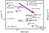 |
Fig. 5 Distribution of properties of 18 optically thick HC H II regions identified in Sect. 4. The vertical and horizontal dotted and dashed lines indicate the standard quantitative criteria of an HC H II region. The red filled circles show HC H II regions and HC H II region candidates identified in this work while the red filled circles with lime circles identify the previously known HC H II regions. The filled blue circles show the intermediate objects between the HC H II andUC H II region stages. The magenta arrow shows the evolutionary trend. |
Summary of the physical parameters and the classification of the 20 optical thick H II regions identified in this work.
G024.7898+0.0833
This source is an HC H II region identified by Beltrán et al. (2007), which is found to be associated with many CH3OH masers (Surcis et al. 2015; Bartkiewicz et al. 2016) and OH masers (Forster & Caswell 2000; Caswell et al. 2013), H2 O masers (Caswell et al. 1983; Forster & Caswell 2000), and outflows traced by CO (Furuya et al. 2002; Beltrán et al. 2011) and SiO (Codella et al. 2013). Its physical properties such as ne, diam, and EM (Table 8) are consistent with previous results (Beltrán et al. 2007; Cesaroni et al. 2019). Its natal clump has a mass of 7.64 × 10³ M⊙ and a bolometric luminosity of 1.58 × 10⁵ L⊙ (Urquhart et al. 2018). The spectral type of this HC H II region O6.5 derived from the infrared luminosity (Table 1) is much earlier than O9.5 derived from the Lyman continuum flux which includes contributions from the nearby UC H II region G024.7889+00.0824 in the field. One possible explanation for the discrepancy of spectral type is that this source is located in a cluster and/or a significant amount of Lyman continuum photons are absorbed by the surrounding dust, with an upper limit on the dust absorption fraction of fd = 92% (see Sects. 3.3.2 and 3.3.3). As this HC H II region shows extended 4.5 μm emission, it is associated with an extended green object as defined by Cyganowski et al. (2008).
G028.2003−0.0494
This source is a known HC H II region identified by Sewilo et al. (2004), which is found to be associated with the 37.7 GHz CH3OH maser (Ellingsen et al. 2011), OH masers (Argon et al. 2000; Caswell et al. 2013), and H2 O masers (Urquhart et al. 2011). Its physical properties such as ne, diam, and EM listed in Table 8 are consistent with previous results (Sewiło et al. 2011). Its natal clump has a mass of 4.45 × 10³ M⊙ and a bolometric luminosity of 1.30 × 10⁵ L⊙ (Urquhart et al. 2018), which is associated with molecular outflows (Maud et al. 2015; Yang et al. 2018). Its spectral type O6.5 derived from the bolometric luminosity is earlier than O7.5 derived from the Lyman continuum flux that includes the contribution from its nearby UC H II region G028.1985−00.0503 with NLy = 5.0 × 1047. This could be the result of this source being located in a cluster, as shown in the middle-left panel of Fig. 6, or could be due to the fact that about 43% of the Lyman continuum photons are absorbed by the surrounding dust.
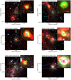 |
Fig. 6 Three-color composition image (or RGB image) from Spitzer GLIMPSE 8 μm (red), 4.5 μm (green), and 3.6 μm (blue) bands (Benjamin et al. 2003; Churchwell et al. 2009) for the HC H II regions discussed in Sect. 4. Lime or red circles show the radio sources in the field from the CORNISH survey. The upper-right zoomed-in images for each panel show the peak position of H2 O maser (magenta cross) and OH maser (black cross), and the linear scale-bar of 0.1 pc in white. Gray contours in the image show 870 μm emission from ATLASGAL (Schuller et al. 2009), and the lime (or red) contours show K-band 22 GHz emission presented in this work. The red contours in the bottom-right panel show X-band 10 GHz emission as the K-band emission is missing for source G045.0694. The FWHM beam of GLIMPSE (2′′) and K-band observationsare indicated by the white circles shown in the lower-left corner of each image. |
G030.0096−00.2734
This compact radio source, located in the W43 star-forming complex (e.g., Blum et al. 1999; Medina et al. 2019; Gao et al. 2019), is the first of the sample that was found to be associated with an infrared dark cloud (G030.01−0.27; Battersby et al. 2011), which itself is associated with many molecular lines (Schlingman et al. 2011) as well as methanol masers (Breen et al. 2015). Its natal clump, AGAL030.008−0.272, is associated with a molecular outflow identified by Yang et al. (2018), which has a maximum outflow velocity of 4.5 km s−1. It is the only radio source in its natal clump, and its spectral type B1 derived from the bolometric luminosity is consistent with B0.5 derived from the Lyman continuum photons, indicating a lack of dust within this H II region. The radio emission is coincident with a compact mid-infrared point source confirming it is associated with an embedded protostellar object. The physical properties of G030.0096−00.2734 are consistent with this source being an HC H II region at a very early evolutionary stage.
G030.5887−00.0428
This source shows compact radio emission at 5 GHz CORNISH, as shown in the middle-right panel of Fig. 8. Its flux densities at high frequencies were obtained in project VLA18A-066, with 217.70 mJy at 15.5 GHz and 223.53 mJy at 16.5 GHz. With flux densities at low frequency of 1.4 and 5 GHz (summarized in Yang et al. 2019), its physical properties can be determined from the radio SED. Water, hydroxyl, and methanol maser sites (Argon et al. 2000; Pestalozzi et al. 2005; Urquhart et al. 2011) are detected in its vicinity, and molecular outflows (Yang et al. 2018) are found to be associated with its natal clump. Its natal clump AGAL030.588−00.042 has a mass of 758 M⊙ and a bolometric luminosity of 1.12 × 10⁴ L⊙ (Urquhart et al. 2018), and shows a broad millimeter RRL H40α with ΔV = 56.2 km s−1 (Kim et al. 2017). It is the only radio source in the parent clump, and its spectral type B0.5, obtained from the bolometric luminosity, is consistent with that of a B0 star derived from the radio luminosity, indicating the absence of dust within this H II region. The broad RRL line, compact size, and high electron density are consistent with this source being classified as an HC H II region.
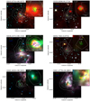 |
Fig. 7 As described in Fig. 6, except in this case the sources include newly identifiedHC H II regions and intermediate objects. The gray contours in the image of G061.4770+00.0892 show the 500μm emission from Hi−GAL. |
G032.7441−00.0755
The radio emission associated with this source is weak and very compact and there is bright emission at 70 μm from the Hi−GAL survey (Molinari et al. 2010), while no counterpart is seen at mid-infrared wavelengths (8 μm; see middle-right panel of Fig. 7). This source was found to host H2 O masers (Caswell et al. 1983), OH masers (Caswell et al. 2013), and CH3OH masers (Bartkiewicz et al. 2016), and is associated with CO outflows (Yang et al. 2018), broad molecular lines such as SiO (2-1) (Csengeri et al. 2016), N2 H+, and HCO+ (Shirley et al. 2013) and millimeter RRLs (ΔV = 40.34 km s−1; Kim et al. 2017). The blueshifted and redshifted methanol masers spots mapped by Bartkiewicz et al. (2016) have a similar orientation to the blueshifted and redshifted outflows mapped by Yang et al. (2018). Its physical parameters (ne = 2.79 × 105 cm−3, diam = 0.011 pc, EM = 8.28 × 10⁸ pc cm−6, νt = 14.37 GHz) are consistent with other HC H II regions and we therefore identify this as a new mid-infrared-dark HC H II region detection. Figure 7 shows that it is the only radio source in its natal clump. Its spectral type O7 derived from the bolometric luminosity is earlier than O9.5 derived from the Lyman continuum flux, indicating that about 88% of the Lyman continuum photons were absorbed by dust within this H II region. It could be the best example to trace the dynamics associated with the final stages of accretion in massive star formation because it is still dark at 8 μm and covers a significant broad component of ionized- (e.g., RRL), shocked- (e.g., SiO), and molecular gas (e.g., CO).
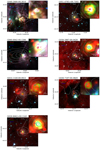 |
Fig. 8 As described in Fig. 6, except in this case the sources are HC H II regions and intermediate objects between HC H II and UC H II regions. The gray contours in the image of G060.8842−00.1286 show the 500μm emission from Hi−GAL. The lime contours in the images of G030.7197−00.0829, G030.8662+00.1143, G030.5887−00.0428 and G33.1328−00.0923 show the 5 GHz emission from CORNISH survey. |
G034.2572, G034.2573 and G034.2581
These three H II regions lie in G34.26+0.15, a well-studied complex region that contains three UC H II regions (Wood & Churchwell 1989; Sewilo et al. 2004): G34.26+0.15A (G034.2573+00.1523), G34.26+0.15B (G034.2581+00.1533) and G34.26+0.15C (G034.2572+00.1535); these are marked with red circles in the middle-left panel of Fig. 7. This complex also hosts H2 O masers (Hofner & Churchwell 1996), OH masers (Forster & Caswell 1999; Ruiz-Velasco et al. 2016), CH3OH masers (Breen et al. 2015) and numerous molecules (Fu & Lin 2016; Kim et al. 2000), as well as infall/outflows traced by CO or water masers (e.g., Wyrowski et al. 2016; van der Tak et al. 2019; Yang et al. 2018; Imai et al. 2011). Broad radio recombination lines (RRLs) are detected in G34.26+0.15B and G34.26+0.15C with a line-width of ΔV > 40 km s−1 (Sewilo et al. 2004). This is also found in their natal clump AGAL034.258+00.154 (Kim et al. 2017, 2018). G34.26+0.15B is considered to be a HC H II region candidate (G034.2581+00.1533, Sewilo et al. 2004; Yang et al. 2019), which is blended with G34.26+0.15C in the C-band and X-band images, and is only resolved in the higher resolution K-band image. G034.2572+00.1535 is associated with G34.26+0.15C, which is an extended source, and can be resolved into three compact sources, all of which have RRL line widths of ΔV > 40 km s−1 (Sewilo et al. 2004).
G034.2572+00.1535 is very likely to host candidates in an evolutionary stage between HC H II region and UC H II region. The nearby source G034.2573+00.1523 is also likelyto be associated with an HC H II region.
G043.1652, G043.1657 and G043.1665
These three sources are located in the well-known star-forming region W49A complex that is associated with CO outflows (Scoville et al. 1986). As shown in the bottom-left panel of Fig. 6, the three sources are associated with three HC H II regions W49A A (G043.1652+00.0129), W49A B (G043.1657+00.0116), and W49A G (G043.1665+00.0106) in the W49A complex (De Pree et al. 1997, 2004; Sewilo et al. 2004), which are found to be associated with many CH3OH (Bartkiewicz et al. 2014; Breen et al. 2015), OH (Argon et al. 2000), and H2 O (De Pree et al. 2000; Urquhart et al. 2011) masers. G043.1657+00.0116 (W49A B) has ne = 1.57 × 105 cm−3, diam = 0.046 pc, EM = 11.32 × 10⁸ pc cm−6, and log NLy = 48.69, which is consistent with the typical value of HC H II regions, as reported by De Pree et al. (2000).
G043.1652+00.0129 (W49A A) is resolved into two compact components at higher resolution ~ 0.05′′ (De Pree et al. 2000, 2004). Its physical properties such as ne = 0.88 × 105 cm−3, diam = 0.053 pc, EM = 4.15 × 10⁸ pc cm−6, and logNLy = 48.91, are consistent with previous results in De Pree et al. (1997) for W49 A at a similar resolution of ~ 1′′. However, the derived properties are slightly below the typical values of HC H II regions and also show smaller ne, smaller EM, and larger diam compared to the results measured at higher resolution (0.05′′) with ne = 6.1 × 105 cm−3, diam = 0.056 pc, and EM = 83 × 108 pc cm−6 (De Pree et al. 2000). This might be due to the fact that our observation includes not only the two compact components but also a larger fraction of optically thin emission around them.
G043.1665+00.0106 (W49A G) is also multiply peaked at higher resolution ~ 0.05′′ (De Pree et al. 2000, 2004). Its physical properties, such as ne = 0.24 × 105 cm−3, diam = 0.24 pc, EM = 1.22 × 10⁸ pc cm−6, and logNLy = 49.55, are consistent with the results in de Pree et al. (1996) for W49A G. The ne is slightly smaller compared to the measurements at higher resolution with ne > 1.0 × 105 cm−3 for the two main compact components (De Pree et al. 2000), which may result from the large amount of optically thin emission around these compact components.
G045.0712 and G045.0694
The radio emission consists of two distinct sources: the stronger source G045.0712+00.1321 and the weaker source G045.0694+00.1323, offset by ~ 6′′ (as shown in bottom-right panel of Fig. 6). G045.0712+00.1321 was identified as an HC H II region by Keto et al. (2008) and Sewiło et al. (2011) (G45.07+0.13 NE). The physical properties ofG045.0712+00.1321 indicate that this HC H II region is associated with a O6.5 type massive star, which supports the previous results and classification by Sewiło et al. (2011). The fainter of the two, G045.0694+00.1323, is likely to be transitioning into an UC H II region based on the distribution of radio properties shown in Fig. 5. Their radio emission is coincident with a bright extended infrared source and a dense submillimeter clump, AGAL045.071+00.132, in Urquhart et al. (2018). The natal clump is associated with extended molecular outflows aligned W to E (Yang et al. 2018). This source is also host to H2 O (Hofner & Churchwell 1996), OH (Argon et al. 2000), and CH3OH masers (Kurtz et al. 2004). The presence of two very young H II regions, molecular outflows, and three different species of masers would suggest that this clump hosts a young proto-cluster.
G045.4656+00.0452
This compact radio source is embedded in a dense molecular clump and is associated with an extended mid-infrared source, as well as water (Forster & Caswell 1999) and OH (Argon et al. 2000) maser emissions (see bottom-left panel of Fig. 7). Its natal clump AGAL045.466+00.046 is also associated with bipolar outflows (Yang et al. 2018) and broad H39α RRL (Δv= 47.8 km s−1; Kim et al. 2017). Cyganowski et al. (2008) identified this source as an extended green object associated with an infrared dark cloud. The physical parameters determined for this source (ne = 1.02 × 105 cm−3, diam = 0.023 pc, EM = 2.36 × 10⁸ pc cm−6, νt = 7.89 GHz) are consistent with this being classified as an HC H II region.
G061.4770+00.0892
This object is very compact with a deconvolved size similar to that of the beam (~ 0.7′′) at K-band, and its radio emission is blended with a nearby cometary UC H II region detected both in 5 GHz CORNISH and X-band observations described in this work. However, the two sources are separated in the high-resolution observations (~ 0.4′′; Wood & Churchwell 1989) and our K-band observations (~ 0.7′′). As shown in the bottom-right panel of Fig. 7, the near-infrared RGB image of this source presents extended 4.5 μm emission and so it could be associated with an extended green object (EGO) as defined by Cyganowski et al. (2008). A bipolar molecular outflow aligned NE to SW (Phillips & Mampaso 1991; White & Fridlund 1992) and water masers (Henkel et al. 1986; Svoboda et al. 2016) are detected toward its parent cloud. Broad RRL components (Garay et al. 1998) and strong OH (1665/67 MHz) absorption (Sarma et al. 2013) are reported towards this source and the other physical properties derived from radio emission indicate that this source is likely to host an HC H II region.
4.2 Intermediate objects between HC H II and UC H II regions
According to their physical properties, there are eight objects located in the evolutionary stages between HC H II regions and UC H II regions in Table 8. Two out of the eight sources (i.e., G034.2572+00.1535 and G045.0694+00.1323) are associated with clusters of H II regions that have already been discussed in Sect. 4.1; in the following sections we provide brief notes on the other six intermediate objects.
G030.7197−00.0829
This source was resolved at 5 GHz by CORNISH. The physical properties (ne = 0.22 × 105 cm−3, diam = 0.09 pc, EM = 0.45 × 10⁸ pc cm−6, νt = 3.6 GHz) can be determined from the radio SED based on flux densities of 464.58 mJy at 1.4 GHz (White et al. 2005), 969.33 mJy at 5 GHz (Purcell et al. 2013), and 570 mJy at 43 GHz (Leto et al. 2009). These results are consistent with the measurements in Leto et al. (2009). Its natal clump AGAL030.718−00.082 has a mass of 6.6 × 10³ M⊙, a bolometric luminosity of 5.5 × 10⁴ L⊙ (Urquhart et al. 2018), and a broad millimeter RRL H40α with ΔV = 43.0 km s−1 (Kim et al. 2017), and is associated with CO outflows (Yang et al. 2018). Its Lyman continuum flux agrees with its bolometric luminosity, indicating a lack of dust within this H II region. Therefore, this source appears to be an intermediate object between HC H II andUC H II regions.
G030.8662+00.1143
The SED of this resolved source was constructed from the flux densities of 137.17 mJy at 1.4 GHz and of 255.2 mJy at 5 GHz from White et al. (2005), 306.0 mJy at 6.7 GHz, and 356.0 mJy at 8.4 GHz from Walsh et al. (1998), as well as 560 mJy at 43 GHz from Leto et al. (2009). Its physical characteristics measured from the radio SED, such as ne = 0.37 × 105 cm−3, diam = 0.03 pc, EM = 0.42 × 10⁸ pc cm−6, and νt =3.5 GHz, are consistent with previous measurements (Leto et al. 2009). Water maser sites (Urquhart et al. 2009b, 2011) are detected in its vicinity and molecular outflows (Yang et al. 2018) are found to be associated with its natal clump. Its natal clump AGAL030.866+00.114 has a mass of 295 M⊙, a bolometric luminosity of 1.30 × 10⁴ L⊙ (Urquhart et al. 2018), and a broad millimeter RRL H39α with ΔV = 44.9 km s−1 (Kim et al. 2017). Its spectral type B0.5 obtained from the bolometric luminosity is consistent with O9.5 derived from radio luminosity, indicating the absence of dust in this H II region. Therefore, this source appears to be an intermediate object.
G033.1328−00.0923
This source shows extended emission at 5 GHz CORNISH, shown as lime contours in the bottom-left panel of Fig. 8. With flux densities of 173.43 mJy at 1.4 GHz and 378.59 mJy at 5 GHz summarized in Yang et al. (2019), as well as 461.2 mJy at 9 GHz and 675.3 mJy at 15 GHz measured by Kurtz et al. (1994), we construct its radio SED between 1 and 15 GHz. Its physical properties from the SED fitting are consistent with results in Kurtz et al. (1994). Water masers (Pestalozzi et al. 2005; Kurtz & Hofner 2005) are detected in its vicinity and molecular outflows (Yang et al. 2018) are found to be associated with its natal clump. Its natal clump AGAL033.133−00.092 has a mass of 5.0 × 10³ M⊙, a bolometric luminosity of 1.1 × 10⁵ L⊙ (Urquhart et al. 2014, 2018), and a broad millimeter RRL H39α with ΔV = 43.0 km s−1 (Kim et al. 2017). As it is only one radio source in the natal clump, its spectral type O7 obtained from the bolometric luminosity is consistent with O7.5 derived from the radio luminosity. Therefore, this source is likely to be an intermediate object between HC H II andUC H II region.
G049.3666−00.3010
This object appears to have a nearby UC H II region to the east referenced as G049.3704−00.3012 (marked with a red circle in the upper-left panel of Fig. 8). Both of these H II regions are embedded towards the center of the dense clump AGAL049.369−00.301, which has been associated with a broad H40α RRL with ΔV = 34.5 km s−1 (Kim et al. 2017). The optically thick radio source is coincident with an extended mid-infrared source, and two water masers have been detected in its vicinity (Valdettaro et al. 2001; Xi et al. 2015).
G051.6785+00.7193
This radio source is very compact at all radio bands presented in this work, while it can be resolved into two sources at high angular resolution ~ 0.2′′ at 1.3 cm using the VLA in Rodríguez-Esnard et al. (2012). The radio source is embedded in a very compact and centrally condensed ATLASGAL clump AGAL051.678+00.719 with a mass of 2.88 × 10³ M⊙ and is associated with a very bright mid-infrared point source that has a luminosity of 1.0 × 10⁵ L⊙. The natal clump is also associated with water and methanol masers (Sridharan et al. 2002; Rodríguez-Esnard et al. 2012), and molecular outflows aligned with extended mid-infrared emission going from NE to SW (Beuther et al. 2004), as presented in the upper-right panel of Fig. 8.
G060.8842−00.1286
This object is southwest of the two H II regions (see middle-left panel of Fig. 8) in the massive star-forming region S87IRS1 (Barsony 1989), the other being a nearby extended and weak H II region (Purcell et al. 2013) that has been resolved out at K-band in this work. The S87IRS1 is associated with the clump JPSG060.886-00.129 in Eden et al. (2017), which is itself associated with a molecular outflow (Barsony 1989; Xue & Wu 2008). The radio source is associated with bright mid-infrared emission and coincident with a water maser (Kurtz & Hofner 2005). At high resolution ~0.4′′, the clump is found to be fragmented into multiple millimeter cores (Beuther et al. 2018). Its bolometric luminosity agrees with its radio luminosity, suggesting a lack of dust within this H II region.
4.3 HC H II regions not resolved in this work
In addition to the optically thick radio sources identified in this work, we include notes on another four HC H II regions that have been identified in previous studies (e.g., Wood & Churchwell 1989, Sewilo et al. 2004 and Zhang et al. 2014) but are unresolved in our observations. Two of the four (G043.1652+00.0129 and G035.5781−00.0305) are unresolved mainly due to the fact that our observations include their nearby UC H II regions as the resolution is not sufficient to resolve the emission into individual sources. The remaining two regions (G043.1665+00.0106 and G010.9584+0.0211) are not recovered by this work primarily because our observations include a large amount of surrounding ionized gas emission as this diffuse gas is optically thin. Therefore, the derived properties in this work represent average values for sources with co-existing emission from HC H II and nearby UC H II regions or represent a complex weighted average over the compact sources plus the surrounding diffuse ionized gas, and thus do not satisfy the criteria for classification as HC H II regions. However, these sources have previously been identified as HC H II regions and we therefore include these sources in this section for completeness. The source names and derived properties are given towards the end of Table 8. Two sources (G043.1652+00.0129 and G043.1665+00.0106) in the W49A complex region have already been discussed together in Sect. 4.1 and are therefore not described again here. Images of the remaining two HC H II regions are presented in Fig. 6 and brief notes are provided below.
G010.9584+0.0221
This source is an HC H II region and is located in the western part of the G10.96+0.01 region and surrounded by more diffuse ionized gas, as suggested by Sewilo et al. (2004). Its physical properties, such as ne = 0.36 × 105 cm−3, diam = 0.029 pc, EM = 0.38 × 10⁸ pc cm−6 and log NLy = 47.35, are all consistent with the results reported by Sewilo et al. (2004) and Sewiło et al. (2011). In spite of the reported broad H92α line with ΔV = 43.8 ± 1.5 km s−1, the derived properties are slightly below the typical values of HC H II regions, which might be due to the previous VLA observations (Sewilo et al. 2004, Sewiło et al. 2011) and this work includes a significant amount of optically thin emission from the diffuse ionized gas around this source, and both results are likely to be underestimates by averaging over the compact source plus its surrounding ionized gas, as mentioned in Sewilo et al. (2004) and Yang et al. (2019). Its natal clump has a mass of 398 M⊙ and a bolometric luminosity of 1.0 × 10⁴ L⊙ (Urquhart et al. 2018), and is associated with high velocity outflow wings identified in CO spectra from the SEDIGISM survey (Schuller et al. 2017). In this case, the luminosity and Lyman continuum flux are both contributed by the same source, meaning that the spectral type derived from the bolometric luminosity is consistent with that derived from the radio luminosity; B0.5 and B0, respectively.
G035.5781−00.0305
This radio emission can be resolved into two extremely close sources at 2 and 3.6 cm with a resolution of < 1′′ (Kurtz et al. 1994): the source to the west has been identified as an HC H II region G35.578−0.030 (Zhang et al. 2014) and the source to the east as an UC H II, G35.578−0.031 (Kurtz et al. 1994). These are seen as a single blended source in our radio maps (see the middle-right panel of Fig. 6). This source is associated with OH masers (Argon et al. 2000) and H2 O masers (Forster & Caswell 1999; Urquhart et al. 2011). The physical properties for the blended source G035.5781−00.0305 are ne = 0.22 × 105 cm−3, diam = 0.093 pc, EM = 0.45 × 10⁸ pc cm−6, and log NLy = 48.36. Thus, G035.5781−00.0305 in this work has smaller ne, smaller EM and larger diam compared to the HC H II region G35.578−0.030 in Zhang et al. (2014) with ne = 3.3 × 105 cm−3, diam = 0.018 pc, EM = 1.9 × 10⁹ pc cm−6. Its natal clump has a mass of 6.8 × 10³ M⊙ and a bolometric luminosity of 2.0 × 10⁵ L⊙ (Urquhart et al. 2018), which is associated with molecular outflows (Yang et al. 2018).
4.4 Summary
In Table 8 we summarize the physical properties of the sources of our sample and the associated discussion in the preceding text. Inspection of this table reveals that in addition to the physical properties (ne, diam, EM and RRL), which are typical for HC H II regions, all the sources of our sample are found to be embedded towards the centres of dense molecular clumps and are also commonly associated with various masers, molecular outflows, broad RRLs, and extended green objects, all of which are all signposts of active star formation. The bolometric luminosities tend to be higher than the radio flux suggests, which is consistent with these being associated with a forming protocluster. These optically thick H II regions are therefore the best examples to investigate the relation between HC H II regions and UC H II regions, to study the birth of H II regions, and therefore to understand the final stages of accretion in massive star formation.
There are 13 HC H II regions, 3 HC H II region candidates, and 8 intermediate objects listed in Table 8. Among them, four HC H II regions and three HC H II region candidates are reported here for the first time. Based on the classification of HC H II regions in Table 7, it is difficult to assess the completeness of the sample of HC H II regions and intermediate H II regions identified in this study because there are four HC H II regions, marked with an asterisk in Table 8, that are in very close proximity to other UC H II regions that we were not able to resolve.
5 Discussion
5.1 Implications of the evolution of young H II regions
As suggested by classical theoretical models (Dyson et al. 1995; Mezger & Henderson 1967), H II regions are expected to expand over time, which results in decreasing ne and EM and increasing diam, as seen in Fig. 5. The plots shown in this figure display a clear evolutionary trend in ne, diam, and EM from HC H II regions to the intermediate objects between the HC H II and UC H II region stages. The mean values of physical properties range from ne = 2.5 × 105 cm−3, diam = 0.012 pc, and EM = 5.5 × 10⁸ pc cm−6 for HC H II regions, to ne = 0.79 × 105 cm−3, diam = 0.03, and EM = 1.58 × 10⁸ pc cm−6 for intermediate objects, and thus ne tends to change quickly compared to the EM and diam at the earliest times of H II region stage.
To investigate the evolution of physical properties of H II regions over a wide range of evolutionary stages, we add the CORNISH UC H II regions from Kalcheva et al. (2018) that are presumably in a later stage compared to our sample. Evolution of the Lyman continuum flux NLy, turnover frequency νt, and emission measure EM is presented in Fig. 9 for the three subsamples discussed here and for the four subsamples by adding the more evolved CORNISH UC H II regions. We see that νt decreases as the H II region evolves, from 11.5 GHz for HC H II regions to 6.4 GHz for intermediate objects, and to 1.8 GHz for UC H II regions, as expected from the theoretical model in Mezger & Henderson (1967). It is interesting to note that there is no obvious correlation between the Lyman continuum flux and the evolution of the H II regions. Furthermore, we find no significant correlation between NLy and EM with ρ = −0.01 and p-value = 0.85, and between NLy and ne with ρ = −0.07 and p-value = 0.3 in the four subsamples. In addition, the mean value of NLy ~ 1048 s−1 is consistent throughout the four evolutionary phases, from the HC H II region and HC H II region candidates, to intermediate objects, to UC H II regions in this work, and to more evolved UC H II regions in CORNISH. These results suggest that there is effectively no evolution of the Lyman continuum photon flux with changes in the νt, ne, and EM, and by extension there is no increase in NLy with evolution of the H II region.
As shown in the bottom-left panel of Fig. 9, the positive correlation between NLy and diam is significant with ρ = 0.5 and p-value ≪ 0.001, using a partial correlation test to control the distance dependence, giving a power-law relation of NLy ∝diam1.4±0.1. However, given the fact that there is little evidence of any sort of significant correlation between Lyman continuum flux and other parameters tracing the evolution of H II regions, such as νt, ne, or EM as discussed above, this correlation is more likely to result from the fact that more luminous H II regions expand more rapidly in their early stages but that the expansion speed will decrease over time, becoming similar to less luminous H II regions. The evolution shown in bottom-left panel of Fig. 9 is therefore from left to right rather than diagonal from bottom-left to upper-right as suggested from the distribution. The flat evolution of NLy indicates that the value of NLy remains constant as the H II region develops, and by extension that the ionizing flux from a young massive star remains constant during the evolutionary phases of H II regions in this sample. This result is in agreement with the classical expansion model without gravity or the model with gravity in Keto (2002) in which the NLy of the H II region tends to stop increasing if it reaches the critical ratios where the accretion is quickly reduced. Also, the constant NLy over time agrees with the results of Hosokawa & Omukai (2009) and Hosokawa et al. (2010) who showed that the luminosity and temperatureof a bloated protostar remain almost unchanged in the last accretion phase. Moreover, the almost unchanged NLy may also supportthe model of Peters et al. (2010) who proposed that a shrinking H II region has small fluctuations of 5–7% in ionizing fluxover time.
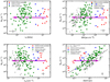 |
Fig. 9 Plots of the evolution and correlation of the derived physical parameters. νt vs. NLy (upper-left), EM vs. NLy (upper-right), ne vs. NLy (bottom-left), and diam vs. NLy (bottom-right) for HC H II regions (red dots), intermediate objects between HC H II region and UC H II regions (blue), UC H II regions in this work (green dots), and CORNISH UC H II regions (gray dots). The CORNISH UC H II regions sample refers to the whole CORNISH UC H II regions sample from Kalcheva et al. (2018) by excluding UC H II regions in this work. The magenta arrow indicates the evolutionary trend of the physical properties. |
5.2 Lyman continuum−bolometric luminosity relationship
The measurements of Lyman continuum flux in the optically thin regime presented in Sect. 3.3.2 and the bolometric luminosity of the sample measured by previous studies (see Table 1) allow us to discuss the relation between Lyman continuum photons (NLy) and bolometric luminosity (Lbol), as well as Lyman continuum flux excess phenomenon in the sample of young H II regions. There exists a significantly positive correlation between Lbol and NLy with ρ = 0.54 and p-value ≪ 0.001 when using the partial correlation test to remove the distance dependence, which is consistent with the correlation (ρ = 0.69) calculated by Urquhart et al. (2013) for a sample of ultra-compact and compact H II regions.
Figure 10 shows NLy as a function of Lbol. The color symbols indicate the physical size of the sample and the black solid line represents the upper limit of the expected Lyman continuum photon rates at specific given bolometric luminosities for ZAMS stars. About 40% of the sources in the sample are located in the forbidden region above this black line, suggesting a Lyman continuum excess. Considering a 50% uncertainty on NLy and Lbol, the fraction of Lyman excess sources in our sample is consistent with ~30% sources in previous work (Sánchez-Monge et al. 2013; Cesaroni et al. 2015). Those sources with Lyman excess are more likely to be associated with young B-type stars (e.g., Sánchez-Monge et al. 2013; Lumsden et al. 2013; Urquhart et al. 2013).
Most of the optically thick H II regions in the sample do not show a Lyman continuum excess; these are marked with red circles in Fig. 10 and located to the right of the black solid line representing the upper limit of the expected Ly continuum photons. The main reason for this is that many are embedded in clusters (as discussed in Sect. 4). Although it is possible that the Lyman flux has been underestimated because of filtering of some of the extended flux in the interferometric observations (e.g., Urquhart et al. 2013), and because of absorption by dust in the H II region (e.g., Wood & Churchwell 1989; Garay et al. 1993), it is unlikely these affects would be significant enough to result in these objects having a Lyman excess (in many cases the Lyman flux would need to have been underestimated by an order of magnitude or more).
It is possible that some of the optically thick objects we have detected are ionized jets whose radio emission also has positive spectral indices (Moscadelli et al. 2016; Purser et al. 2016), and because there are very weak (Sint ~ mJy) and compact (diam ~ 1000 AU) sources (see Sect. 4). We include the empirical relationship between bolometric luminosity (Lbol) and Lyman flux (NLy) derived from young stellar objects (YSOs) in Fig. 10 (dotted diagonal line; Purser et al. 2016). Given that it is likely that the Lyman continuum flux has been underestimated and the bolometric luminosity has been overestimated, only the optically thick sources located to the right of this relation are associated with radio jets; these are G030.0096, G060.8842, G034.2573, G034.2581, and G061.4770. The radio emission of the five sources are point-like as shown in Figs. 7 and 8, and therefore no morphological evidence was found to indicate that they are radio jets, which implies that they are more likely to be HC H II regions as discussed in Sect. 4. Further observations are needed to reliably classify these objects.
In Fig. 10, there are seven young H II regions in Table 8 located close to the black solid line, namely G010.9584, G030.0096, G030.5887, G030.8662, G060.8842, G030.7197, and G033.1328, which means that their Lyman continuum fluxes agree well with their bolometric luminosities, and further indicates the absence of dust within these H II regions to absorb the Lyman continuum photons. These seven objects are the only radio sources in the observed field of this work and in their parent clumps from Urquhart et al. (2018). Three of the seven (G010.9584, G030.0096, and G030.5887) have been suggested to be in the HC H II region stage and the remaining four are expected to be in the intermediate stage between HC H II and UC H II regions. Except for three sources with no RRL information, the remaining five sources show broad RRL with line widths ΔV > 40 km s−1, and all of them are associated with outflows and masers, as shown in Table 8. These dust-free and young H II regions are interesting cases to study the destruction of dust in the very young H II regions because H II regions are often expected to be dusty in the early stages, as discussed in Sect. 3.3.3 and in Arthur et al. (2004). Further investigations are needed to understand the absence of dust in these young H II regions.
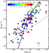 |
Fig. 10 Lyman continuum flux NLy vs. the bolometric luminosity Lbol for young H II regions with rising spectra. The black solid line refers to the expected Lyman continuumphoton rate from a single ZAMS star of a given bolometric luminosity. The top axis lists the spectral type corresponding to a given bolometric luminosity taken from stellar models (Thompson 1984; Panagia 1973; Davies et al. 2011). The error bars in the bottom-right corner correspond to a 50% uncertainty for Lbol and NLy (Urquhart et al. 2018). At the top, we show the color bar for the physical size of the sources, indicating the physical diameter in parsecs. The red circles and black squares refer to optically thick H II regions (νt > 5 GHz) and optically thin H II regions (νt < 5 GHz). About 30% of the sample is located in the forbidden region above the solid curve considering a 50% uncertainty. The dotted line represents the empirical relation between Lbol and NLy for ionized jets from YSOs, with a power-law index of 0.64 derived by Purser et al. (2016). The red arrows for the optically thick H II regions indicate that the bolometric luminosities are upper limits due to the presence of other H II regions in the same clump. |
6 Summary and conclusion
In this work, we report the results of multi-band (8–12 and 18–26 GHz), high angular-resolution (~ 1.7′′ and ~ 0.7′′), VLA observations toward a sample of young H II regions that are selected on the basis of rising spectra between 1 and 5 GHz in Yang et al. (2019). We construct their radio SED between 1 and 26 GHz and measure their physical properties for 116 young H II regions by modeling each SED based on an ionization-bounded H II region with standard uniform electron density. The sample has a mean electron density of 1.6 × 104 cm−3, a mean diameter of 0.14 pc, a mean emission measure of 1.9 × 10⁷pc cm−6, a mean turnover frequency of 3.29 GHz, and a mean Lyman continuum flux of 6.5 × 1047 s−1. Based on these properties, there are a total of 20 HC H II regions and 3 candidates reported so far after combining our findings with the HCH ii region catalog summarized in Yang et al. (2019). This sample consists of a large number of HC H II regions and UC H II regions, which gives us a comprehensive picture of the physical condition and evolution of these young H II regions. The main resultsof our study can be summarized as follows:
- 1.
We identify 16 HC H II regions and 8 intermediate objects located between the class of HC H II and UC H II regions. Four HC H II regions and three candidates are newly reported in this work, along with two new infrared-dark HC H II regions.
- 2.
We discuss how the physical properties of H II regions change as they evolve from HC H II regions to UC H II regions and then to compact H II regions. While ne, diam, EM, and νt all change during this evolution, the Lyman continuum flux stays relatively constant over time, suggesting that the accretion tends to be quickly reduced or could be halted at the earliest HC H II region stage in our sample.
- 3.
These young and compact H II regions are located in dusty clumps. The mean fraction of ionizing flux absorbed by dust in H II regions is 67%, and the absorption fraction tends to be more significant for the more compact and younger H II regions. Nevertheless, about 40% of the sources show Lyman continuum excess and are preferentially associated with young B-type stars.
In conclusion, young H II regions are likely to be located in dusty clumps. The youngest H II regions, namely HC H II regions and intermediate objects between HC H II and UC H II, are found to be associated with star-forming activity such as that found in various masers, molecular outflows, broad RRLs, and extended green objects. Accretion at the two earliest stages of H II region evolution tends to be quickly reduced or stopped, and therefore these regions could be optimal tracers of the final stages of massive star formation.
Acknowledgements
We would like to thank the anonymous referee for the helpful comments. A.Y.Y. thanks Yan Gong for his helpful discussion. W.W.T. acknowledges support from the National Key R&D Programs of China (2018YFA0404203). This work has made use of the SIMBAD database (CDS, Strasbourg, France). The VLA is operated by the National Radio Astronomy Observatory, which is a facility of the National Science Foundation operated under cooperative agreement by Associated Universities, Inc.
References
- Afflerbach, A., Churchwell, E., Acord, J. M., et al. 1996, ApJS, 106, 423 [NASA ADS] [CrossRef] [Google Scholar]
- Argon, A. L., Reid, M. J., & Menten, K. M. 2000, ApJS, 129, 159 [NASA ADS] [CrossRef] [Google Scholar]
- Arthur, S. J., Kurtz, S. E., Franco, J., & Albarrán, M. Y. 2004, ApJ, 608, 282 [NASA ADS] [CrossRef] [Google Scholar]
- Avalos, M., Lizano, S., Rodríguez, L. F., Franco-Hernández, R., & Moran, J. M. 2006, ApJ, 641, 406 [NASA ADS] [CrossRef] [Google Scholar]
- Barsony, M. 1989, ApJ, 345, 268 [NASA ADS] [CrossRef] [Google Scholar]
- Bartkiewicz, A., Szymczak, M., & van Langevelde, H. J. 2014, A&A, 564, A110 [NASA ADS] [CrossRef] [EDP Sciences] [Google Scholar]
- Bartkiewicz, A., Szymczak, M., & van Langevelde, H. J. 2016, A&A, 587, A104 [NASA ADS] [CrossRef] [EDP Sciences] [Google Scholar]
- Battersby, C., Bally, J., Ginsburg, A., et al. 2011, A&A, 535, A128 [NASA ADS] [CrossRef] [EDP Sciences] [Google Scholar]
- Beltrán, M. T., Cesaroni, R., Moscadelli, L., & Codella, C. 2007, A&A, 471, L13 [NASA ADS] [CrossRef] [EDP Sciences] [Google Scholar]
- Beltrán, M. T., Cesaroni, R., Zhang, Q., et al. 2011, A&A, 532, A91 [CrossRef] [EDP Sciences] [Google Scholar]
- Benjamin, R. A., Churchwell, E., Babler, B. L., et al. 2003, PASP, 115, 953 [NASA ADS] [CrossRef] [Google Scholar]
- Beuther, H., Schilke, P., & Gueth, F. 2004, ApJ, 608, 330 [NASA ADS] [CrossRef] [Google Scholar]
- Beuther, H., Bihr, S., Rugel, M., et al. 2016, A&A, 595, A32 [NASA ADS] [CrossRef] [EDP Sciences] [Google Scholar]
- Beuther, H., Mottram, J. C., Ahmadi, A., et al. 2018, A&A, 617, A100 [NASA ADS] [CrossRef] [EDP Sciences] [Google Scholar]
- Bihr, S., Johnston, K. G., Beuther, H., et al. 2016, A&A, 588, A97 [NASA ADS] [CrossRef] [EDP Sciences] [Google Scholar]
- Bisbas, T. G., Haworth, T. J., Williams, R. J. R., et al. 2015, MNRAS, 453, 1324 [NASA ADS] [CrossRef] [MathSciNet] [Google Scholar]
- Blum, R. D., Damineli, A., & Conti, P. S. 1999, AJ, 117, 1392 [NASA ADS] [CrossRef] [Google Scholar]
- Breen, S. L., Fuller, G. A., Caswell, J. L., et al. 2015, MNRAS, 450, 4109 [NASA ADS] [CrossRef] [Google Scholar]
- Carey, S. J., Noriega-Crespo, A., Mizuno, D. R., et al. 2009, PASP, 121, 76 [NASA ADS] [CrossRef] [Google Scholar]
- Caswell, J. L., Batchelor, R. A., Forster, J. R., & Wellington, K. J. 1983, Aust. J. Phys., 36, 443 [NASA ADS] [CrossRef] [Google Scholar]
- Caswell, J. L., Green, J. A., & Phillips, C. J. 2013, MNRAS, 431, 1180 [NASA ADS] [CrossRef] [Google Scholar]
- Cesaroni, R., Pestalozzi, M., Beltrán, M. T., et al. 2015, A&A, 579, A71 [NASA ADS] [CrossRef] [EDP Sciences] [Google Scholar]
- Cesaroni, R., Beltrán, M. T., Moscadelli, L., Sánchez-Monge, Á., & Neri, R. 2019, A&A, 624, A100 [NASA ADS] [CrossRef] [EDP Sciences] [Google Scholar]
- Churchwell, E., Babler, B. L., Meade, M. R., et al. 2009, PASP, 121, 213 [NASA ADS] [CrossRef] [Google Scholar]
- Codella, C., Beltrán, M. T., Cesaroni, R., et al. 2013, A&A, 550, A81 [NASA ADS] [CrossRef] [EDP Sciences] [Google Scholar]
- Contreras, Y., Schuller, F., Urquhart, J. S., et al. 2013, A&A, 549, A45 [NASA ADS] [CrossRef] [EDP Sciences] [Google Scholar]
- Csengeri, T., Leurini, S., Wyrowski, F., et al. 2016, A&A, 586, A149 [NASA ADS] [CrossRef] [EDP Sciences] [Google Scholar]
- Cyganowski, C. J., Whitney, B. A., Holden, E., et al. 2008, AJ, 136, 2391 [NASA ADS] [CrossRef] [Google Scholar]
- Davies, B., Hoare, M. G., Lumsden, S. L., et al. 2011, MNRAS, 416, 972 [NASA ADS] [CrossRef] [Google Scholar]
- de Pree, C. G., Gaume, R. A., Goss, W. M., & Claussen, M. J. 1996, ApJ, 464, 788 [CrossRef] [Google Scholar]
- De Pree, C. G., Mehringer, D. M., & Goss, W. M. 1997, ApJ, 482, 307 [NASA ADS] [CrossRef] [Google Scholar]
- De Pree, C. G., Wilner, D. J., Goss, W. M., Welch, W. J., & McGrath, E. 2000, ApJ, 540, 308 [NASA ADS] [CrossRef] [Google Scholar]
- De Pree, C. G., Wilner, D. J., Mercer, A. J., et al. 2004, ApJ, 600, 286 [NASA ADS] [CrossRef] [Google Scholar]
- Djordjevic, J. O., Thompson, M. A., Urquhart, J. S., & Forbrich, J. 2019, MNRAS, 487, 1057 [NASA ADS] [Google Scholar]
- Dyson, J. E., & Williams, D. A. 1997, The Physics of the Interstellar Medium, 2nd edn. (Bristol: Institute of Physics Publishing) [CrossRef] [Google Scholar]
- Dyson, J. E., Williams, R. J. R., & Redman, M. P. 1995, MNRAS, 277, 700 [NASA ADS] [Google Scholar]
- Eden, D. J., Moore, T. J. T., Plume, R., et al. 2017, MNRAS, 469, 2163 [NASA ADS] [CrossRef] [Google Scholar]
- Ellingsen, S. P., Breen, S. L., Sobolev, A. M., et al. 2011, ApJ, 742, 109 [NASA ADS] [CrossRef] [Google Scholar]
- Forster, J. R., & Caswell, J. L. 1999, A&AS, 137, 43 [NASA ADS] [CrossRef] [EDP Sciences] [Google Scholar]
- Forster, J. R., & Caswell, J. L. 2000, ApJ, 530, 371 [NASA ADS] [CrossRef] [Google Scholar]
- Fu, L., & Lin, G.-M. 2016, Res. A&A, 16, 182 [Google Scholar]
- Furuya, R. S., Cesaroni, R., Codella, C., et al. 2002, A&A, 390, L1 [NASA ADS] [CrossRef] [EDP Sciences] [Google Scholar]
- Gao, X. Y., Reich, P., Hou, L. G., Reich, W., & Han, J. L. 2019, A&A, 623, A105 [CrossRef] [EDP Sciences] [Google Scholar]
- Garay, G., & Lizano, S. 1999, PASP, 111, 1049 [NASA ADS] [CrossRef] [Google Scholar]
- Garay, G., Rodriguez, L. F., Moran, J. M., & Churchwell, E. 1993, ApJ, 418, 368 [NASA ADS] [CrossRef] [Google Scholar]
- Garay, G., Lizano, S., Gómez, Y., & Brown, R. L. 1998, ApJ, 501, 710 [NASA ADS] [CrossRef] [Google Scholar]
- Gibb, A. G., & Hoare, M. G. 2007, MNRAS, 380, 246 [NASA ADS] [CrossRef] [Google Scholar]
- Hatchell, J., Thompson, M. A., Millar, T. J., & MacDonald, G. H. 1998, A&AS, 133, 29 [NASA ADS] [CrossRef] [EDP Sciences] [Google Scholar]
- Helfand, D. J., Becker, R. H., White, R. L., Fallon, A., & Tuttle, S. 2006, AJ, 131, 2525 [NASA ADS] [CrossRef] [Google Scholar]
- Henkel, C., Haschick, A. D., & Guesten, R. 1986, A&A, 165, 197 [Google Scholar]
- Hoare, M. G., Kurtz, S. E., Lizano, S., Keto, E., & Hofner, P. 2007, Protostars and Planets V (Tucson, AZ: University of Arizona Press), 181 [Google Scholar]
- Hoare, M. G., Purcell, C. R., Churchwell, E. B., et al. 2012, PASP, 124, 939 [NASA ADS] [CrossRef] [Google Scholar]
- Hofner, P., & Churchwell, E. 1996, A&AS, 120, 283 [NASA ADS] [CrossRef] [EDP Sciences] [Google Scholar]
- Hollenbach, D., Johnstone, D., Lizano, S., & Shu, F. 1994, ApJ, 428, 654 [NASA ADS] [CrossRef] [Google Scholar]
- Hosokawa, T., & Omukai, K. 2009, ApJ, 691, 823 [NASA ADS] [CrossRef] [Google Scholar]
- Hosokawa, T., Yorke, H. W., & Omukai, K. 2010, ApJ, 721, 478 [NASA ADS] [CrossRef] [Google Scholar]
- Imai, H., Omi,R., Kurayama, T., et al. 2011, PASJ, 63, 1293 [NASA ADS] [CrossRef] [Google Scholar]
- Kalcheva, I. E., Hoare, M. G., Urquhart, J. S., et al. 2018, A&A, 615, A103 [NASA ADS] [CrossRef] [EDP Sciences] [Google Scholar]
- Keto, E. 2002, ApJ, 580, 980 [NASA ADS] [CrossRef] [Google Scholar]
- Keto, E. 2003, ApJ, 599, 1196 [NASA ADS] [CrossRef] [Google Scholar]
- Keto, E. 2007, ApJ, 666, 976 [NASA ADS] [CrossRef] [Google Scholar]
- Keto, E., & Wood, K. 2006, ApJ, 637, 850 [NASA ADS] [CrossRef] [Google Scholar]
- Keto, E., Zhang, Q., & Kurtz, S. 2008, ApJ, 672, 423 [NASA ADS] [CrossRef] [Google Scholar]
- Kim, K.-T., & Koo, B.-C. 2001, ApJ, 549, 979 [NASA ADS] [CrossRef] [Google Scholar]
- Kim, H.-D., Cho, S.-H., Chung, H.-S., et al. 2000, ApJS, 131, 483 [NASA ADS] [CrossRef] [Google Scholar]
- Kim, W.-J., Wyrowski, F., Urquhart, J. S., Menten, K. M., & Csengeri, T. 2017, A&A, 602, A37 [NASA ADS] [CrossRef] [EDP Sciences] [Google Scholar]
- Kim, W. J., Urquhart, J. S., Wyrowski, F., Menten, K. M., & Csengeri, T. 2018, A&A, 616, A107 [NASA ADS] [CrossRef] [EDP Sciences] [Google Scholar]
- König, C., Urquhart, J. S., Csengeri, T., et al. 2017, A&A, 599, A139 [NASA ADS] [CrossRef] [EDP Sciences] [Google Scholar]
- Kurtz, S. 2005, IAU Symp., 227, 111 [NASA ADS] [CrossRef] [Google Scholar]
- Kurtz, S., & Hofner, P. 2005, AJ, 130, 711 [NASA ADS] [CrossRef] [Google Scholar]
- Kurtz, S., Churchwell, E., & Wood, D. O. S. 1994, ApJS, 91, 659 [NASA ADS] [CrossRef] [Google Scholar]
- Kurtz, S., Cesaroni, R., Churchwell, E., Hofner, P., & Walmsley, C. M. 2000, Protostars and Planets IV (Tucson, AZ: University of Arizona Press), 299 [Google Scholar]
- Kurtz, S., Hofner, P., & Álvarez, C. V. 2004, ApJS, 155, 149 [NASA ADS] [CrossRef] [Google Scholar]
- Leto, P., Umana, G., Trigilio, C., et al. 2009, A&A, 507, 1467 [NASA ADS] [CrossRef] [EDP Sciences] [Google Scholar]
- López-Sepulcre, A., Codella, C., Cesaroni, R., Marcelino, N., & Walmsley, C. M. 2009, A&A, 499, 811 [NASA ADS] [CrossRef] [EDP Sciences] [Google Scholar]
- Lumsden, S. L., Hoare, M. G., Urquhart, J. S., et al. 2013, ApJS, 208, 11 [NASA ADS] [CrossRef] [Google Scholar]
- Maud, L. T., Moore, T. J. T., Lumsden, S. L., et al. 2015, MNRAS, 453, 645 [NASA ADS] [CrossRef] [Google Scholar]
- McKee, C. F., & Tan, J. C. 2003, ApJ, 585, 850 [NASA ADS] [CrossRef] [MathSciNet] [Google Scholar]
- McMullin, J. P., Waters, B., Schiebel, D., Young, W., & Golap, K. 2007, ASP Conf. Ser., 376, 127 [Google Scholar]
- Medina, S. N. X., Urquhart, J. S., Dzib, S. A., et al. 2019, A&A, 627, A175 [CrossRef] [EDP Sciences] [Google Scholar]
- Mezger, P. G., & Henderson, A. P. 1967, ApJ, 147, 471 [NASA ADS] [CrossRef] [Google Scholar]
- Molinari, S., Swinyard, B., Bally, J., et al. 2010, PASP, 122, 314 [NASA ADS] [CrossRef] [Google Scholar]
- Moscadelli, L., Sánchez-Monge, Á., Goddi, C., et al. 2016, A&A, 585, A71 [NASA ADS] [CrossRef] [EDP Sciences] [Google Scholar]
- Motte, F., Bontemps, S., & Louvet, F. 2018, ARA&A, 56, 41 [NASA ADS] [CrossRef] [Google Scholar]
- Murphy, T., Cohen, M., Ekers, R. D., et al. 2010, MNRAS, 405, 1560 [Google Scholar]
- Panagia, N. 1973, AJ, 78, 929 [NASA ADS] [CrossRef] [Google Scholar]
- Panagia, N., & Felli, M. 1975, A&A, 39, 1 [Google Scholar]
- Pascucci, I., Apai, D., Henning, T., Stecklum, B., & Brandl, B. 2004, A&A, 426, 523 [NASA ADS] [CrossRef] [EDP Sciences] [Google Scholar]
- Pestalozzi, M. R., Minier, V., & Booth, R. S. 2005, A&A, 432, 737 [NASA ADS] [CrossRef] [EDP Sciences] [Google Scholar]
- Peters, T., Banerjee, R., Klessen, R. S., et al. 2010, ApJ, 711, 1017 [NASA ADS] [CrossRef] [Google Scholar]
- Phillips, J. P.,& Mampaso, A. 1991, A&AS, 88, 189 [Google Scholar]
- Purcell, C. R., Hoare, M. G., Cotton, W. D., et al. 2013, ApJS, 205, 1 [NASA ADS] [CrossRef] [Google Scholar]
- Purser, S. J. D., Lumsden, S. L., Hoare, M. G., et al. 2016, MNRAS, 460, 1039 [NASA ADS] [CrossRef] [Google Scholar]
- Rodríguez-Esnard, T., Trinidad, M. A., & Migenes, V. 2012, ApJ, 761, 158 [CrossRef] [Google Scholar]
- Ruiz-Velasco, A. E., Felli, D., Migenes, V., & Wiggins, B. K. 2016, ApJ, 822, 101 [NASA ADS] [CrossRef] [Google Scholar]
- Sánchez-Monge, Á., Beltrán, M. T., Cesaroni, R., et al. 2013, A&A, 550, A21 [NASA ADS] [CrossRef] [EDP Sciences] [Google Scholar]
- Sarma, A. P., Brogan, C. L., Bourke, T. L., Eftimova, M., & Troland, T. H. 2013, ApJ, 767, 24 [CrossRef] [Google Scholar]
- Schlingman, W. M., Shirley, Y. L., Schenk, D. E., et al. 2011, ApJS, 195, 14 [NASA ADS] [CrossRef] [Google Scholar]
- Schuller, F., Menten, K. M., Contreras, Y., et al. 2009, A&A, 504, 415 [NASA ADS] [CrossRef] [EDP Sciences] [Google Scholar]
- Schuller, F., Csengeri, T., Urquhart, J. S., et al. 2017, A&A, 601, A124 [NASA ADS] [CrossRef] [EDP Sciences] [Google Scholar]
- Scoville, N. Z., Sargent, A. I., Sanders, D. B., et al. 1986, ApJ, 303, 416 [NASA ADS] [CrossRef] [Google Scholar]
- Sewilo, M., Churchwell, E., Kurtz, S., Goss, W. M., & Hofner, P. 2004, ApJ, 605, 285 [NASA ADS] [CrossRef] [Google Scholar]
- Sewiło, M., Churchwell, E., Kurtz, S., Goss, W. M., & Hofner, P. 2011, ApJS, 194, 44 [NASA ADS] [CrossRef] [Google Scholar]
- Shirley, Y. L., Ellsworth-Bowers, T. P., Svoboda, B., et al. 2013, ApJS, 209, 2 [NASA ADS] [CrossRef] [Google Scholar]
- Spitzer, L. 1978, Physical Processes in the Interstellar Medium (Wiley-VCH Verlag GmbH & Co. KGaA) [Google Scholar]
- Sridharan, T. K., Beuther, H., Schilke, P., Menten, K. M., & Wyrowski, F. 2002, ApJ, 566, 931 [NASA ADS] [CrossRef] [Google Scholar]
- Steggles, H. G. 2016, PhD thesis, University of Leeds, UK [Google Scholar]
- Steggles, H. G., Hoare, M. G., & Pittard, J. M. 2017, MNRAS, 466, 4573 [NASA ADS] [CrossRef] [Google Scholar]
- Surcis, G., Vlemmings, W. H. T., van Langevelde, H. J., et al. 2015, A&A, 578, A102 [NASA ADS] [CrossRef] [EDP Sciences] [Google Scholar]
- Svoboda, B. E., Shirley, Y. L., Battersby, C., et al. 2016, ApJ, 822, 59 [NASA ADS] [CrossRef] [Google Scholar]
- Thompson, R. I. 1984, ApJ, 283, 165 [NASA ADS] [CrossRef] [Google Scholar]
- Thompson, M. A., Hatchell, J., Walsh, A. J., MacDonald, G. H., & Millar, T. J. 2006, A&A, 453, 1003 [NASA ADS] [CrossRef] [EDP Sciences] [Google Scholar]
- Thompson, M., Beuther, H., Dickinson, C., et al. 2015, Advancing Astrophysics with the Square Kilometre Array (AASKA14), 126 [CrossRef] [Google Scholar]
- Thompson, M., Goedhart, S., Goedhart, S., et al. 2016, MeerKAT Science: On the Pathway to the SKA, 15 [Google Scholar]
- Urquhart, J. S., Busfield, A. L., Hoare, M. G., et al. 2007, A&A, 461, 11 [NASA ADS] [CrossRef] [EDP Sciences] [Google Scholar]
- Urquhart, J. S., Hoare, M. G., Purcell, C. R., et al. 2009a, A&A, 501, 539 [NASA ADS] [CrossRef] [EDP Sciences] [Google Scholar]
- Urquhart, J. S., Hoare, M. G., Lumsden, S. L., et al. 2009b, A&A, 507, 795 [NASA ADS] [CrossRef] [EDP Sciences] [Google Scholar]
- Urquhart, J. S., Morgan, L. K., Figura, C. C., et al. 2011, MNRAS, 418, 1689 [NASA ADS] [CrossRef] [Google Scholar]
- Urquhart, J. S., Thompson, M. A., Moore, T. J. T., et al. 2013, MNRAS, 435, 400 [NASA ADS] [CrossRef] [Google Scholar]
- Urquhart, J. S., Csengeri, T., Wyrowski, F., et al. 2014, A&A, 568, A41 [NASA ADS] [CrossRef] [EDP Sciences] [Google Scholar]
- Urquhart, J. S., König, C., Giannetti, A., et al. 2018, MNRAS, 473, 1059 [NASA ADS] [CrossRef] [Google Scholar]
- Valdettaro, R., Palla, F., Brand, J., et al. 2001, A&A, 368, 845 [NASA ADS] [CrossRef] [EDP Sciences] [Google Scholar]
- van der Tak, F. F. S., & Menten, K. M. 2005, A&A, 437, 947 [NASA ADS] [CrossRef] [EDP Sciences] [Google Scholar]
- van der Tak, F. F. S., Shipman, R. F., Jacq, T., et al. 2019, A&A, 625, A103 [Google Scholar]
- Walsh, A. J., Burton, M. G., Hyland, A. R., & Robinson, G. 1998, MNRAS, 301, 640 [NASA ADS] [CrossRef] [Google Scholar]
- White, G. J., & Fridlund, C. V. M. 1992, A&A, 266, 452 [Google Scholar]
- White, R. L., Becker, R. H., & Helfand, D. J. 2005, AJ, 130, 586 [NASA ADS] [CrossRef] [Google Scholar]
- Wood, D. O. S., & Churchwell, E. 1989, ApJS, 69, 831 [NASA ADS] [CrossRef] [Google Scholar]
- Wyrowski, F., Güsten, R., Menten, K. M., et al. 2016, A&A, 585, A149 [NASA ADS] [CrossRef] [EDP Sciences] [Google Scholar]
- Xi, H., Zhou, J., Esimbek, J., et al. 2015, MNRAS, 453, 4203 [NASA ADS] [CrossRef] [Google Scholar]
- Xue, R., & Wu, Y. 2008, ApJ, 680, 446 [NASA ADS] [CrossRef] [Google Scholar]
- Yang, A. Y., Tian, W. W., Zhu, H., Leahy, D. A., & Wu, D. 2016, ApJS, 223, 6 [CrossRef] [Google Scholar]
- Yang, A. Y., Thompson, M. A., Urquhart, J. S., & Tian, W. W. 2018, ApJS, 235, 3 [NASA ADS] [CrossRef] [Google Scholar]
- Yang, A. Y., Thompson, M. A., Tian, W. W., et al. 2019, MNRAS, 482, 2681 [NASA ADS] [CrossRef] [Google Scholar]
- Zhang, C.-P., Wang, J.-J., Xu, J.-L., Wyrowski, F., & Menten, K. M. 2014, ApJ, 784, 107 [NASA ADS] [CrossRef] [Google Scholar]
- Zinnecker, H., & Yorke, H. W. 2007, ARA&A, 45, 481 [NASA ADS] [CrossRef] [Google Scholar]
The Karl G. Jansky Very Large Array of the National Radio Astronomy Observatory: https://science.nrao.edu/facilities/vla
This study by Urquhart et al. (2018) is based on the ATLASGAL compact source catalog, which consists of ~10 000 clumps showing submillimeter wavelength emission from dust (Contreras et al. 2013; Urquhart et al. 2014).
All Tables
Observational results of 112 young H II regions at X-band (8–12 GHz) and K-band (18–26 GHz).
Summary of observational results and the derived physical parameters for 116 young H II regions.
Summary of the derived physical parameters for the 96 optically thin H II regions (νt < 5 GHz) and the 20 optically thick H II regions (νt > 5 GHz).
Quantitative criteria for HC H II regions, UC H II regions and intermediate objects (HC H II → UC H II) between the two stages, summarized from the literature.
Summary of the physical parameters and the classification of the 20 optical thick H II regions identified in this work.
All Figures
|
Fig. 1 Example images of three radio sources at C-band (left-column), X-band (middle-column), and K-band (right-column). The position of the H II region is marked with a plus. Upper, middle, and lower rows: maps for the compact H II region G032.7441−00.0755, the extendedH ii region G035.4669+00.1394, and the H II region G043.1665+00.0106 located in a cluster (see Sect. 3.1), respectively. C-band images are from the CORNISH survey. The white contour levels of each image are equally spaced by 5σ and start at a level of 5σ. The green outline shown in the lower row shows the polygon that was manually drawn around the H II region located in acluster. The image size and beam size are shown in the upper-middle and lower-left of each image. The C-band, X-band, and K-band images for the whole sample are available in electronic form at the Zenodo via https://doi.org/10.5281/zenodo.4293684. |
| In the text | |
|
Fig. 2 Distributions of observation results such as integrated flux density Sint, peak flux density Speak, and angular size θ, of 116 young H II regions at X-band (blue solid line) and K-band (red solid line). The bin sizes are 0.5 dex, 0.5 dex, and 1′′ for Sint, Speak, and θ, respectively. |
| In the text | |
|
Fig. 3 Radio SED fitting to flux density points for example compact and extended sources. Upper panel: SED fitting to flux density points between 1 and 26 GHz for the compact example G032.7441−00.0755 (upper row of Fig. 1). Lower panel: SED fitting to flux density points between 1 and 11 GHz for extended example G035.4669+00.1394 (middle row of Fig. 1) by excluding K-band flux measurements. The best-fitting results for the electron density ne and physical linear diameter diam are shown in the upper-left corner of each plot. The best-fitting SEDs for the whole sample are available in electronic form at the Zenodo via https://doi.org/10.5281/zenodo. 4293684. |
| In the text | |
|
Fig. 4 Distributions of the derived physical properties of 116 young H II regions. Panels a–c: distributions of the physical linear diameter diam (a), the electron density ne (b), and the EM (c). The bin sizesare 0.05 pc, 0.25 dex, and 0.25 dex for diam, ne, and EM, respectively. Panels d–f: distributions of the turnover frequency νt (d), the Lyman continuum flux NLy (e), and the dust absorption fraction fd (f). The bin sizesare 0.1, 0.1, and 0.5 dex for νt, fd, and NLy, respectively. |
| In the text | |
|
Fig. 5 Distribution of properties of 18 optically thick HC H II regions identified in Sect. 4. The vertical and horizontal dotted and dashed lines indicate the standard quantitative criteria of an HC H II region. The red filled circles show HC H II regions and HC H II region candidates identified in this work while the red filled circles with lime circles identify the previously known HC H II regions. The filled blue circles show the intermediate objects between the HC H II andUC H II region stages. The magenta arrow shows the evolutionary trend. |
| In the text | |
|
Fig. 6 Three-color composition image (or RGB image) from Spitzer GLIMPSE 8 μm (red), 4.5 μm (green), and 3.6 μm (blue) bands (Benjamin et al. 2003; Churchwell et al. 2009) for the HC H II regions discussed in Sect. 4. Lime or red circles show the radio sources in the field from the CORNISH survey. The upper-right zoomed-in images for each panel show the peak position of H2 O maser (magenta cross) and OH maser (black cross), and the linear scale-bar of 0.1 pc in white. Gray contours in the image show 870 μm emission from ATLASGAL (Schuller et al. 2009), and the lime (or red) contours show K-band 22 GHz emission presented in this work. The red contours in the bottom-right panel show X-band 10 GHz emission as the K-band emission is missing for source G045.0694. The FWHM beam of GLIMPSE (2′′) and K-band observationsare indicated by the white circles shown in the lower-left corner of each image. |
| In the text | |
|
Fig. 7 As described in Fig. 6, except in this case the sources include newly identifiedHC H II regions and intermediate objects. The gray contours in the image of G061.4770+00.0892 show the 500μm emission from Hi−GAL. |
| In the text | |
|
Fig. 8 As described in Fig. 6, except in this case the sources are HC H II regions and intermediate objects between HC H II and UC H II regions. The gray contours in the image of G060.8842−00.1286 show the 500μm emission from Hi−GAL. The lime contours in the images of G030.7197−00.0829, G030.8662+00.1143, G030.5887−00.0428 and G33.1328−00.0923 show the 5 GHz emission from CORNISH survey. |
| In the text | |
|
Fig. 9 Plots of the evolution and correlation of the derived physical parameters. νt vs. NLy (upper-left), EM vs. NLy (upper-right), ne vs. NLy (bottom-left), and diam vs. NLy (bottom-right) for HC H II regions (red dots), intermediate objects between HC H II region and UC H II regions (blue), UC H II regions in this work (green dots), and CORNISH UC H II regions (gray dots). The CORNISH UC H II regions sample refers to the whole CORNISH UC H II regions sample from Kalcheva et al. (2018) by excluding UC H II regions in this work. The magenta arrow indicates the evolutionary trend of the physical properties. |
| In the text | |
|
Fig. 10 Lyman continuum flux NLy vs. the bolometric luminosity Lbol for young H II regions with rising spectra. The black solid line refers to the expected Lyman continuumphoton rate from a single ZAMS star of a given bolometric luminosity. The top axis lists the spectral type corresponding to a given bolometric luminosity taken from stellar models (Thompson 1984; Panagia 1973; Davies et al. 2011). The error bars in the bottom-right corner correspond to a 50% uncertainty for Lbol and NLy (Urquhart et al. 2018). At the top, we show the color bar for the physical size of the sources, indicating the physical diameter in parsecs. The red circles and black squares refer to optically thick H II regions (νt > 5 GHz) and optically thin H II regions (νt < 5 GHz). About 30% of the sample is located in the forbidden region above the solid curve considering a 50% uncertainty. The dotted line represents the empirical relation between Lbol and NLy for ionized jets from YSOs, with a power-law index of 0.64 derived by Purser et al. (2016). The red arrows for the optically thick H II regions indicate that the bolometric luminosities are upper limits due to the presence of other H II regions in the same clump. |
| In the text | |
Current usage metrics show cumulative count of Article Views (full-text article views including HTML views, PDF and ePub downloads, according to the available data) and Abstracts Views on Vision4Press platform.
Data correspond to usage on the plateform after 2015. The current usage metrics is available 48-96 hours after online publication and is updated daily on week days.
Initial download of the metrics may take a while.