| Issue |
A&A
Volume 645, January 2021
|
|
|---|---|---|
| Article Number | A27 | |
| Number of page(s) | 27 | |
| Section | Interstellar and circumstellar matter | |
| DOI | https://doi.org/10.1051/0004-6361/202037871 | |
| Published online | 23 December 2020 | |
Quantitative inference of the H2 column densities from 3 mm molecular emission: case study towards Orion B★
1
Laboratoire d’Astrophysique de Bordeaux, Univ. Bordeaux, CNRS, B18N, Allee Geoffroy Saint-Hilaire,
33615 Pessac,
France
e-mail: This email address is being protected from spambots. You need JavaScript enabled to view it.
2
IRAM,
300 rue de la Piscine,
38406 Saint Martin d’Hères,
France
3
LERMA, Observatoire de Paris, PSL Research University, CNRS, Sorbonne Universités,
75014 Paris, France
4
LERMA, Observatoire de Paris, PSL Research University, CNRS, Sorbonne Universités,
92190 Meudon, France
5
Aix-Marseille Univ, CNRS, Centrale Marseille, Institut Fresnel, Marseille,
France
6
Chalmers University of Technology, Department of Space, Earth and Environment,
412 93 Gothenburg, Sweden
7
University of Toulouse, IRIT/INP-ENSEEIHT, CNRS,
2 rue Charles Camichel, BP 7122,
31071 Toulouse cedex 7, France
8
Univ. Grenoble Alpes, Inria, CNRS, Grenoble INP, GIPSA-Lab,
Grenoble
38000,
France
9
Univ. Lille, CNRS, Centrale Lille, UMR 9189 - CRIStAL,
59651 Villeneuve d’Ascq, France
10
Instituto de Física Fundamental (CSIC). Calle Serrano 121,
28006
Madrid,
Spain
11
Instituto de Astrofísica, Pontificia Universidad Católica de Chile,
Av. Vicuña Mackenna 4860,
7820436 Macul,
Santiago, Chile
12
Institut de Recherche en Astrophysique et Planétologie (IRAP), Université Paul Sabatier,
Toulouse cedex 4, France
13
Laboratoire de Physique de l’Ecole normale supérieure, ENS, Université PSL, CNRS, Sorbonne Université, Université Paris- Diderot, Sorbonne Paris Cité,
Paris,
France
14
National Radio Astronomy Observatory,
520 Edgemont Road,
Charlottesville,
VA,
22903, USA
15
School of Physics and Astronomy, Cardiff University,
Queen’s buildings,
Cardiff CF24 3AA, UK
Received:
3
March
2020
Accepted:
25
August
2020
Abstract
Context. Based on the finding that molecular hydrogen is unobservable in cold molecular clouds, the column density measurements of molecular gas currently rely either on dust emission observation in the far-infrared, which requires space telescopes, or on star counting, which is limited in angular resolution by the stellar density. The (sub)millimeter observations of numerous trace molecules can be effective using ground-based telescopes, but the relationship between the emission of one molecular line and the H2 column density is non-linear and sensitive to excitation conditions, optical depths, and abundance variations due to the underlying physico- chemistry.
Aims. We aim to use multi-molecule line emission to infer the H2 molecular column density from radio observations.
Methods. We propose a data-driven approach to determine the H2 gas column densities from radio molecular line observations. We use supervised machine-learning methods (random forest) on wide-field hyperspectral IRAM-30m observations of the Orion B molecular cloud to train a predictor of the H2 column density, using a limited set of molecular lines between 72 and 116 GHz as input, and the Herschel-based dust-derived column densities as “ground truth” output.
Results. For conditions similar to those of the Orion B molecular cloud, we obtained predictions of the H2 column density within a typical factor of 1.2 from the Herschel-based column density estimates. A global analysis of the contributions of the different lines to the predictions show that the most important lines are 13CO(1–0), 12CO(1–0), C18O(1–0), and HCO+(1–0). A detailed analysis distinguishing between diffuse, translucent, filamentary, and dense core conditions show that the importance of these four lines depends on the regime, and that it is recommended that the N2H+(1–0) and CH3OH(20–10) lines be added for the prediction of the H2 column density in dense core conditions.
Conclusions. This article opens a promising avenue for advancing direct inferencing of important physical parameters from the molecular line emission in the millimeter domain. The next step will be to attempt to infer several parameters simultaneously (e.g., the column density and far-UV illumination field) to further test the method.
Key words: methods: statistical / ISM: clouds / ISM: molecules
Data are only available at the CDS via anonymous ftp to cdsarc.u-strasbg.fr (130.79.128.5) or via http://cdsarc.u-strasbg.fr/viz-bin/cat/J/A+A/645/A27
© P. Gratier et al. 2020
 Open Access article, published by EDP Sciences, under the terms of the Creative Commons Attribution License (https://creativecommons.org/licenses/by/4.0), which permits unrestricted use, distribution, and reproduction in any medium, provided the original work is properly cited.
1 Introduction
Atoms and molecules have long been thought to be versatile tracers of the cold neutral medium in the Universe, from high-redshift galaxies to star-forming regions and protoplanetary disks because their internal degrees of freedom bear a signature that reveals clues about the physical conditions of their environments. Atoms and molecules are affected by many processes: photoionization and photodissociation by far-UV photons, excitation by collisions with neutrals and electrons, radiative pumping of excited levels by far-UV or IR photons, gas phase chemical reactions, condensation on grains, solid state reactions in the formed ice, (non)-thermal desorption, etc. Moreover, this chemical activity is tightly coupled with gas dynamics. Chemistry affects the gas motions because (1) the ionization state controls the coupling to the magnetic field; and (2) the line radiation from molecules (mostly rotational lines) and atoms (fine structure lines in the far-IR) is the main cooling agent of theneutral gas over a broad range of astrophysical environments, controlling the equation of state and therefore affecting the dynamics. Conversely, the gas dynamics affects the chemistry because it produces steep and time-variable density and velocity gradients, which change the rates of molecule formation and destruction. Numerical models of interstellar clouds face the difficulty of combining sophisticated chemical codes (addressing the molecule formation and destruction processes) with turbulent gas dynamics. This is a tremendous challenge given the non-linearity of fluid dynamics, the rigidity of chemical reactions, and the wide range of time scales involved (Valdivia et al. 2017; Clark et al. 2019). It is, therefore, important to acquire self-consistent data sets that can be used as templates for this theoretical work and, at the same time, to document the diagnostic capabilities of molecular lines accurately.
The recent development of spectrometers in the (sub)-millimeter domain (e.g., IRAM-30m/EMIR, NOEMA, ALMA) opens new avenues to fulfill this goal. First, wide band spectrometers now allow us to simultaneously observe tens of lines instead of a single one along each line of sight. The first studies using these capabilities were sensitive (~ 3−8 mK) unbiased spectral surveys at 1, 2, and 3 mm targeting a few specific lines of sight (e.g., Horsehead WHISPER: Pety et al. 2012, TMC1: Gratier et al. 2016, ASAI: Lefloch et al. 2018). Firstly, these studies show the power of multi-line studies to constrain the physics and the chemistry of molecular clouds. Secondly, the increase in sensitivity now makes it possible to detect these lines over large areas (several square degrees), paving the way for an era of quasi systematic hyperspectral imaging in the millimeter domain. The ORION-B project (Outstanding Radio-Imaging of OrioN-B, co-PIs: J. Pety and M. Gerin) is a IRAM Large Project using the 30m telescope that aims to improve the understanding of the physical and chemical processes of the interstellar medium by mapping a large fraction of the Orion B molecular cloud (5 square degrees) with a typical resolution of 27″(~ 50 mpc at 400 pc, the typical distance to the Orion B cloud) and 200 kHz (or 0.6 km s−1) over the full 3 mm atmospheric band.
In an early study, Pety et al. (2017) showed how tracers of different optical depths like the CO isotopologues allow us to fully trace the molecular medium, from the diffuse envelope to the dense cores, while various chemical tracers can be used to reveal different environments. However, extracting the information contained in these multi-line observations requires powerful statistical tools. A clustering algorithm applied to the intensities of selected molecular lines revealed spatially continuous regions with similar molecular emission properties, corresponding to different regimes of volume density or far-UV illumination (Bron et al. 2018). In addition, a global principal component analysis of the line integrated brightnesses revealed that some combinations of lines are sensitive to the column density, the volume density, and the UV field (Gratier et al. 2017). In this paper, we go one step further by checking whether it would be possible to build a quantitative estimate of the H2 column density and if so, how that could be done, based on the molecular emission and valid over a large range of conditions. Indeed, this is a prerequisite to classify the interstellar medium into its different phases such as diffuse, translucent, and dense regimes (Pety et al. 2017), and to identify its underlying structure, in particular, its filamentary nature (André et al. 2010; Orkisz et al. 2019). Such a method could also be used to estimate the mass of the different (velocity-separated) components of a giant molecular cloud, for instance, the linear mass of the filaments relative to their more diffuse environment. The H2 column density is also required to compute molecular abundances from observed molecular column densities and compare these with the outputs of astrochemical codes.
To do this, we focus on supervised learning methods. Supervised learning is a general set of machine learning methods used to learn how to assign a class or infer the value of a given quantity from a set of measured observables. These methods need a training set for which we know both the measured features and the searched class or value. Here, we use: (1) the emission of selected spectral lines over a fraction of the observed field of view as input observables; and (2) the dust-traced column density as a proxy of the gas column density. Indeed, multi-wavelength observations of dust thermal emission in the submillimeter range and the subsequent fit of the spectral energy distribution is one of the most successful methods for deriving total column density maps of the interstellar medium. Between 2009 and 2015, the Herschel Observatory instruments PACS (70, 100, 160 μm) and SPIRE (250, 350, 500 μm) mapped a fraction of the sky with an angular resolution of ~40″ or better. In particular, large programmes have been dedicated to this task, for example, the HiGal survey mapping of the inner Galactic plane (68° > l > −70° and |b| < 1° Molinari et al. 2016), or the Gould Belt survey (André et al. 2010). However, since the end of the Herschel mission, and until its potential successor SPICA that could be launched in the 2030s, only SOFIA/HAWK+ is currently able to measure the far-IR dust emission. Ground-based or ballon-borne submillimeter telescopes will map the interstellar medium with even higher angular resolution but the lack of data at shorter wavelengths will make the estimation of the dust temperature highly uncertain. This means that dust temperatures would have to be approximated when deriving the dust-traced column density. This method will likely lead to systematic errors. Hence, devising an accurate method for estimating the H2 column density, which only relies on ground-based (sub-)millimeter facilities, is important.
This paper is structured as follows. Section 2 introduces the data sets and Sect. 3 formalizes the problem. Section 4 introduces our concepts and methods. Section 5 discusses how we applied them in practice. Section 6 compares the performances of different methods. Section 7 discusses which lines are the most important for inferring the H2 column density. Section 8 presents a discussion on whether the column density predictor can be used on noisier data or on data from sources more distant from the Sun than Orion. In this section, we also discuss how the method can be generalized to other physical parameters, such as the far-UV illumination. Section 9 presents our conclusions.
Spectral properties of the observed lines.
2 Data
2.1 Molecular emission from IRAM-30m observations
The acquisition and reduction of the molecular data set used in this study is presented in detail in Pety et al. (2017), but the field of view has been extended to the North and East by ~ 60%. In short, the data were acquired at the IRAM-30m telescope by the ORION-B project in only three frequency tunings: the first from 92.0 to 99.8 GHz (LSB band) and from 107.7 to 115.5 GHz (USB band); the second from 84.5 to 92.3 GHz (LSB band) and from 100.2 to 108.0 GHz (USB band); and the third from 71.0 to 78.8 GHz (LSB band) and from 86.7 to 94.4 GHz (USB band). The data were acquired from August 2013 to February 2015 for the two first tunings and in August 2016 for the third tuning.
The selection of the studied lines was performed based on the spectra averaged over the observed field of view. Table 1 lists the 18 selected lines and their associated tuning setup. A velocity interval of 80 km s−1 was extracted around each line and the spectral axis was resampled onto a common velocity grid. The systemic velocity of the source is set to 10.5 km s−1 and the channel spacing is set to 0.5 km s−1, which is the highest velocity resolution achieved for the 12CO (1− 0) line. This impliesthat the noise is more and more correlated from one channel to the next as the rest frequency of the line decreases.
The studied field of view covers 0.9° × 1.6° towards the Orion B molecular cloud part that contains the Horsehead nebula, and the H II regions NGC 2023, NGC 2024, IC 434, and IC 435. Compared to Pety et al. (2017), Gratier et al. (2017), Orkisz et al. (2017), Bron et al. (2018), it additionally comprises the northern molecular edge that contains the hummingbird filament studied in Orkisz et al. (2019). All the cubes were gridded onto the same spatial grid to ease the analysis. The projection center is located on the Horsehead at  . The maps are rotated counter-clockwise by 14° around this position. The angular resolution ranges from 22.5 to 35.6″. The position-position-velocity cubes of each line were smoothed to a common angular resolution of 40″ to avoid resolution effects during the analysis. This was done by convolution with a Gaussian kernel of width
  where θbeam is the telescope beam for each observed line in arcsec. A pixel size of 20″ was used to ensure Nyquist sampling and to avoid too strong correlations between pixels. At a distance of 400 pc (Menten et al. 2007; Zucker et al. 2019, 2020), the sampled linear scales range from ~80 mpc to ~ 11 pc.
From the position-position-velocity cubes, we computed maps of both the peak temperature and the integrated intensity (moment 0)1. The peak temperature is just the maximum of the spectrum intensity over the 80 km s−1 velocity range. The integrated intensity is computed over a velocity window that is decided as follows. Starting from the peak intensity velocity, all adjacent channels whose intensity is larger than zero are added to the velocity window (Pety 1999). This process is iterated five times, each time starting from the next intensity maximum. Up to five velocity components may, hence, be present on each line of sight.
While the line integrated intensity can be used as a proxy for the column density of the species along the line of sight, at least for some column density interval, we also include the line peak temperature to take into account the possible effect of the excitation temperature on the relationship between the column density and the integrated intensity. As discussed by Pety et al. (2017), we expect variations of the gas temperature (and thus of the excitation temperature) across the targeted field of view because it is exposed to the intense far-UV illumination produced by young OB stars in the more or less embedded H II regions. For optically thick lines, the line peak temperature can be viewed as a proxy for the line excitation temperature where the brightness temperature approaches the excitation temperature. For an (faint) optically thin line, the map of peak temperature is proportional to the excitation temperature times the column density per velocity bin. Using both the line area and the peak temperature partly lifts the degeneracy between excitation and amount of gas along the line of sight (see e.g., the companion article by Roueff et al. 2020).
2.2 N(H2) column density derived from dust thermal emission observed with Herschel
To get an independent measurement of the column density for the Orion B cloud, we use the dust continuum observations from the Herschel Gould Belt Survey (André et al. 2010; Schneider et al. 2013) and from the Planck satellite (Planck Collaboration I 2011). The fit of the spectral energy distribution by Lombardi et al. (2014) gives us access to the spatial distributions of the dust opacity at 850 μm and of the effective dust temperature. As in Pety et al. (2017), we converted τ850 μm to visual extinctions using AV = 2.7 × 10⁴ τ850 mag, and we use NH∕AV = 1.8 × 1021 cm−2 mag−1 as conversion factor between visual extinction and hydrogen column density:  . Over the observed field of view, the column density of atomic hydrogen accounts for less than one visual magnitude of extinction (Pety et al. 2017). We thus choose to neglect this contribution in this study. Figure 1 shows the spatial distribution of this dust-traced column density.
We do not claim that the dust-traced column density used here is a perfect measure of the underlying N(H2) column density. We just wish to check whether the molecular emission alone is able to predict this dust-traced column density. If this method is efficient, the next step will be to anchor it on additional sources of information (see Sect. 8.5).
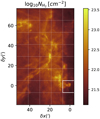 |
Fig. 1 Spatial distribution of the dust-traced H2 column density derived from Herschel data (André et al. 2010; Lombardi et al. 2014). The dotted grid is used to define the training and test sets. The white square in the bottom right around the Horsehead region corresponds to the test set where the random forest predictions will be compared to the observations. This subset is never used during the training phase. Only the remainder of the map is used as the training set. |
2.3 Information content
Figures 2 and 3 show the spatial distribution of the input variables (integrated intensities and peak temperatures of the lines) and target variable (the dust-traced H2 column density). Table 2 lists, among other properties, the minimum and maximum values of the peak temperature maps for the 18 selected lines, as well as the derived dynamic range computed as the ratio of the maximum over the minimum value. The dynamic range spans values between ~ 20 and ~ 700. The dynamic range of the column density is ~400.
The input and targeted variables have different noise properties. Indeed, the dust-traced H2 column density is derived at high signal-to-noise ratio (S/N) over the full field of view. We can safely assume that the targetedvariable is noiseless even though it may be affected by systematic biases in its derivation. On the contrary, large fractions of the field of view is measured at low S/N of the input variables. This is particularly clear on the maps of the peak temperature, which emphasize the noise pattern at S/N lower than 3. The noise pattern suggests that setups #1 and #2 were mainly observed through vertical scanning, while setup #3 was only observed through horizontal scanning. It also suggests non-negligible variations of the noise levels either because of the weather (mostly summer versus winter weather but also degrading weather during one observing session) or because of the large variation of the telescope elevation between the beginning and the end of an observing session.
3 Astrophysical goal: to determine whether it is possible to accurately predict the H2 column density based on molecular emission
Figure 10 of Pety et al. (2017) shows the joint distributions of the dust visual extinction (proportional to the dust-traced column density of matter along the line of sight,  ) and of the line integrated intensity (Wl) for a selection of the detected lines, l. This figure shows a clear monotonic relationship with low scatter between
  and Wl for most of the lines. On one hand, there often exists an interval of column densities for which the relationship between
  and Wl is linear to a good approximation for one line, but the column density interval depends on the line. On the other hand, these relationships are in general non-linear. This is clear when looking at the relationship between
  and
and  . The integrated intensity stays undetected at low column density and it saturates at high column density. This property is generic for any single molecular line, implying that setting up a predictor of the column density from a single line will always fail in some regime.
Taking into consideration that: (1) the relationships between  and Wl are monotonic; and (2) the interval of column densities over which
  ∝ Wl to first order depends on the line, this opens up the interesting possibility that a joint analysis of the molecular lines could allow us to devise a predictor of the column density. Building on these empirical facts, Gratier et al. (2017) applied the simplest global analysis of the existing correlations in a multi-dimensional data set, that is, the principal component analysis. Figure 10 from Gratier et al. (2017) shows the joint histogram of the first principal component and the dust-traced column density. This histogram shows a tight correlation between these two quantities with a Spearman’s rank correlation of 0.90 over more than two orders of magnitude in column density, from 1021 to 1023 H2 cm−2. Moreover, this correlation does not saturate any more at either low or high column density. However, it is not exactly linear.
We now assume that there exists a non-linear continuous function F of the line intensities that predicts the dust-traced column density. Our goal in this article is to quantitatively estimate an approximation (noted f) of this function, F. This estimation will be affected by S/N issues since the line intensity measurements are limited by the sensitivity of the observations, that is, our measurements are generally done at an intermediate S/N. We can write our estimation problem as
 (1)
(1)
where Tl, Wl is the vector of the peak temperatures and integrated intensities of lines l, and e represents the sum of all uncertainties. In this estimation problem, the measurements may also suffer from systematic biases. For instance, the dust-traced column density may underestimate the amount of matter along the line of sight when the emission from warm dust hides the emission from colder dust (Pagani et al. 2015). In the absence of a more quantitative knowledge of such systematic biases, they cannot be separated from the physical relationship in the estimation, f. They will therefore be de facto included in the function, f, which we try to recover.
Getting an accurate estimate of the H2 column density from molecular line emissions is a long-standing quest in the study of stellar formation. Methods followed the development of (sub)millimeter telescopes, receivers, and spectrometers. They can be divided into two main categories. The first category relies on an empirical linear relationship between the H2 column density and the integrated emission of the (1–0) line of the most abundant tracer of molecular gas, namely, 12CO. Bolatto et al. (2013) explain that this method, known as the XCO-factor method, relies on the fact that giant molecular clouds seem, on average, close to the virial equilibrium. The statistical nature of the basis for this method implies that it mostly works at relatively large linear scale (≳10−50 pc). Several studies (Leroy et al. 2011; Genzel et al. 2012) have shown that the XCO factor depends on the metallicity of the inter-stellar medium to take into account varying fraction of CO dark gas, i.e., H2 gas without enough dust to shield the destruction of CO from the surrounding far UV field.
The second category of methods invert a radiative transfer model to obtain the column density of the associated molecular species from the line intensities or observed spectra. Chemical models estimating the abundances relative to H2 are then used to infer  from the molecular column densities. This method is usually applied on the main CO isotopologues. In this category, Dickman (1978); Dickman et al. (1986) derived the mean 13CO abundance relative to H2. Frerking et al. (1982), Bachiller & Cernicharo (1986) and Cernicharo & Guelin (1987) expanded to other CO isotopologues, showing that the threshold for detecting C18O is higher than that for 12CO or 13CO. Goldsmith et al. (2008) and Pineda et al. (2010) used a modified version with a variable [CO]/[H2] abundance ratio deduced from the Black and van Dishoeck PDR models (see e.g., Visser et al. 2009). By comparing 12CO and 13CO (1–0) emission maps with dust extinction maps, Ripple et al. (2013) showed that the relationship between the 13CO column density and Av is non-linear, indicating variations of the 13CO abundance. Barnes et al. (2018) analyzed a recent large survey of the main CO isotopologues to determine a
  -dependent XCO conversion factor. Their analysis assumes that the excitation temperature is the same for the 12CO and 13CO lines, as well as a constant [13CO]/[12CO] abundance. These two assumptions are shown to be incorrect at least in the Orion B molecular cloud by Bron et al. (2018) and Roueff et al. (2020).
In summary, the first category pursues a a direct connection between the line intensity and the H2 column density, while the second category relies on the estimation of the species abundances. Beam filling factor may be an issue in the latter category if it changes the apparent abundance. The current study belongs to the first category.
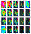 |
Fig. 2 Spatial distribution of the line integrated intensity for some of the detected lines in the 3 mm band, plus the dust-traced far-UV illumination (bottom left panel) and the dust-traced H2 column density (top right corner). The color-scales are logarithmic to reveal the distribution of faint signal and positive noise. The maps are rotated counter-clockwise by 14 degrees from the RA/Dec J2000 reference frame. The spatial offsets are given in arcsecond from the projection center located at |
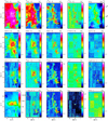 |
Fig. 3 Spatial distribution of the line peak temperature for some of the detected lines in the 3 mm band, plus the dust-traced far-UV illumination (bottom left panel) and the dust-traced H2 column density (top right corner). The color-scales are logarithmic to reveal the distribution of faint signal and positive noise. The maps are rotated counter-clockwise by 14 degrees from the RA/Dec J2000 reference frame. The spatial offsets are given in arcsecond from the projection center located at |
Observed spectral lines and dust-traced properties.
4 Principle: regression in machine learning
In this section, we briefly define the different machine-learning concepts that we use later in this article. It is mostly an intuitive presentation aimed at astronomers who don’t necessarily have a background in machine-learning methods. The main algorithm we use in this paper is called random forest, which was invented by Leo Breiman. Details of its theoretical basis can be found in Breiman (2001)2. An introduction can be found in Hastie et al. (2001, Chap. 15).
4.1 Supervised machine-learning method called regression
Trying to solve Eq. (1) for an approximation of F is a generic machine-learning class of problems known as regression. This approximation of F, which we note as f, is called the regression model. The quantity to be predicted is often called the “dependent” or “target” variable. In our case, it will be the dust-traced column density. The function variables (that is, the observables) are often called “features.” In our case, these will be the measured molecular integrated intensities and peak temperatures. Each line of sight (image pixel) constitutes one measurement of Eq. (1). The regression consists in finding an estimate of F based on the data set. It is a “supervised” method, meaning that it needs to be trained on a dataset for which the solution of the problem is known before the trained method is applied to other datasets.
4.2 Training set, test set, and quality of fit
We use a standard supervised learning workflow by first dividing the full data set into a “training set,” comprising the majority of the observed data on which the best internal parameters of the model are fitted, and a “test set,” which is not seen by the fitting or training algorithm. The quality of the fit is checked by computing the mean square error (MSE) between the value predicted by the model and the observed quantity. There are two kinds of MSE. On one hand, the training MSE is used to fit the model on the training set. On the other hand, the test MSE is computed to assess how the model behaves with regard to data it has not been trained on.
While the regression fit minimizes the training MSE, the final goal is to predict correct values for samples outside of the training set, that is, to minimize the “test” MSE. Small test and training MSE values are expected when the model function is estimated well. This indicates that the model can predict the dust-traced column density based on the values of the molecular intensities on data that have never been used during the fitting procedure. However, finding a test MSE that is much larger than the training MSE is a symptom of a problem known as “overfitting.” In this case, the estimated model function learned not only the searched underlying physics, but also the specifics of the data set measurements, in particular, the noise properties. This can occur, for instance, when the model complexity (i.e., the number of unknown parameters) is too large compared to the information content of the data.
4.3 Variance and bias of the model estimation
The accuracy of the fitted model, that is, achieving the minimum test MSE, always results from a trade-off between the varianceand the bias of the estimated model function (see Sect. 7.3 of Hastie et al. 2001 and Sect. 3.2 of Bishop 2006).
The variance refers to the amount of variation that would affect our estimate of F if the training data set was different. There are different causes of variability in the estimation of F. Firstly, the training set may cover only part of the relevant physical conditions. In our case, we could have failed to sample one of the different column density regimes well enough: either the diffuse or translucent gas, dense cores, etc. Secondly, the condition of the observations, for example, the S/N, can be different from one training set to another.
The bias refers to the fact that there can be a mismatch between the actual complexity of F and the complexity implied by a choice of function family. No matter the amount of data you have in your training sample, trying to fit a non-linear function by an hyper-plane will result in a bias.
Minimizing the test MSE requires selecting a supervised learning method that will find the best trade-off between the variance and the bias. Achieving a low bias but a high variance is easy: any model that goes through all the points of the training data set will do this; it is then completely dependent on the specific noise of the training set and, thus, it is overfitted. Conversely, achieving a low variance but a high bias is just as easy: using the mean of the training data set as model will give this result. The challenge is to find the optimal trade-off between the variance and the bias. As a function of model complexity, variance is minimized at zero complexity and bias is minimized at infinite complexity (or one that is large enough to be an interpolation).
4.4 Decreasing the regressor variance through bagging
Bagging is one of the two standard algorithms used to decrease the variance of a regression method. The other one, called boosting, is not treated in this article. Bagging is an abbreviation for bootstrap aggregating. It is thus related to the bootstrap method, which is often used in astrophysics to estimate random uncertainties in properties inferred from a given data set.
The bootstrap method randomly creates a large number of subsamples of the input data set. In this drawing, replacement is authorized, meaning that the same data point can be chosen multiple times. A regression is then carried out on each sub-sample and the predicted values are computed for each point of each subsample. The aggregation part computes the average of all the predictions. This average becomes the predicted model. It is intuitive to assume that the reduction of the variance comes from the averaging process. This, nevertheless, also assumes that the errors of individual models are uncorrelated. The bias is conserved in this algorithm. In particular, a low bias method will give a low-bias bagged method. A practical advantage of bagging is that it is easily parallelisable, implying short computation times.
4.5 Regression trees
Regression trees are a type of regression method that uses a recursive set of binary splitting on the values of the input variables to estimate thetarget variable. The choice of the split point is made to minimize a cost function. To put it simply, the regression tree poses a series of binary questions to the data, each question narrowing the possible prediction until the method gains enough confidence to assert that this prediction is the right one.
To explain in further detail, at one dimension, the training set is made of couples (xi, yi) that are linked by a to-be-estimated function, f, and the residuals, ei:
 (2)
(2)
The function, f, is an approximation of the data in the form of a step function with steps of variable heights and lengths. To obtain it, the method explores all the potential ways to split the values of the x axis into two categories. For each potential split, it computes the MSE of the two resulting classes. It then chooses the split value that minimizes the average of the two MSE weighted by the number of elements in each class. The outcome of this process is a threshold value of x that splits the data set into two classes called tree branches. The decision point is a node of the tree. The process is then iterated in each branch leading to new nodes and branches. The process is stopped when the maximum depth of the tree is reached or a branch contains less than a given number of data points. The predicted value is then computed as the mean of the y values for these points. The first decision point is called the root node. By construction, it’s the one that reduces the final MSE the most. It is called the strongest predictor. A generalization to a multi-dimensional function is straightforward. All the dimensions are split one after the other and the first decision is made along the dimension that minimizes the weighted average of the MSE of the two resulting branches.
Regression trees have several advantages. They make no assumption, either on the basis of the functional form of the learned relationship or on the shape of the underlying probability density of the data set. They thus belong to the class of non-parametric methods. Regression trees are non-linear regressors by nature. They are easy to understand and, thus, to interpret. In particular, the relative importance of the features is easy to extract. Finally, they do not require any normalization nor centring of the data. This last point is a key advantage for us as Gratier et al. (2017) showed that normalization is difficult when the S/N is low for a number of features.
Regression trees, nevertheless, have several drawbacks. A large tree depth brings high flexibility and thus ensures a low bias, but it also makes these trees prone to overfitting. They are unstable, meaning that a small variation in the training set can lead to a completely different regression tree. This implies that their variance is large and that there is no guarantee that the outcome is the globally optimal regression tree. However, most of the drawbacks can be overcome by using a random forest method.
4.6 Random forest
A random forest can overcome the instability and high variance of a regression tree by averaging the predictions from many such trees that include two sources of randomness. First, the input data set is bootstrapped. However, introducing only this kind of randomness would produce highly correlated trees in case the data set contains several strong predictors (i.e., a split decision along a given dimension that largely decreases the MSE). Indeed, these strong predictors will be consistently chosen at the top levels of the tree. So, random forests introduce a second source of randomness at each decision point: instead of minimising the MSE along all the dimensions, it minimizes it along a random subset of the dimensions. Hence, a random forest is a regression method made of bagged regression trees (first kind of randomness) that are split on random subsets of features at each split (second kind of randomness). This not only reduces the variance but it also speeds up the computations because the introduction of randomness is done on both a subset of the data and a subset of the dimensions.
4.7 Model complexity versus interpretability
Later in thispaper, we show that linear regressors fall short in capturing all of the non-linearities of the relationships between molecular emission and N(H2) column density. This calls for a more flexible method. Neural networks are a well-known example of a method that performs well in complex machine learning tasks (see, e.g., Boucaud et al. 2020) but the interpretation of their output is usually difficult. Having an interpretable result is an important criterion for us as we aim to understand the properties of the interstellar medium. Firstly, we put more confidence in the predictions if the interpretation is physically and chemically sound. Secondly, the learned relationships between features and predicted values should provide meaningful insights into the physical and chemical properties of the molecular interstellar medium. Random forests represent a good compromise in complexity versus interpretability as they are able to learn non-linear relationships while keeping the properties that make physical interpretation possible and that allow us to understand a posteriori how the predictions have been obtained.
5 Application
The random forest implementation that we use is the RandomForestRegressor class from the sklearn python module (Pedregosa et al. 2011).
5.1 Quality of the regression and generalization: mean error and RMSE
We monitor the quality of the regressor and its generalization power by computing the mean error and the root mean square error (RMSE) either on the test or training sets. To do this, we compute the residuals, that is, the difference between the observed and predicted values of the column density for each pixel, and then we compute its mean and RMSE. The RMSE quantifies the distance between the observations and the predictions, while the mean error informs us on potential global biases of the regressors and predictors.
While the mean square error (MSE) is used in machine learning because it is simpler and, thus, makes it faster to compute as it does not involve the computation of the square root, the results we present from this point on use the root mean square error. This choice enables us to have values that can be directly compared to the predicted quantity and it gives to first order an estimation of the uncertainty on the predictions. Moreover, there is no loss of generality as the square root is a monotonous function.
5.2 Separation of the data into training and test sets
The molecular emission is spatially coherent over a large number of pixels for two reasons. First, Nyquist sampling implies that neighbor pixels are correlated. Second, the underlying physical properties of the molecular emission are spatially correlated across pixels. Standard methods to divide the data sets into training and test sets, which are based on random draws of the observations, would lead to two correlated sets, weakening the results obtained on the test set. Furthermore, choosing a test region where the physical and chemical properties are well-known is desirable to ease the interpretation of the regression results. Figure 1 shows our choice of training and test sets. We divide the observed region into 40 rectangles of 12.7′ × 13.3′ or 38 × 40 pixels.
The test set is chosen as the rectangle containing the Horsehead Nebula, which has been extensively studied (Pety et al. 2005, 2012; Goicoechea et al. 2006; Gerin et al. 2009; Guzmán et al. 2011, 2012; Gratier et al. 2013; Fuente et al. 2017) and is shown as a bold white rectangle in Fig. 1. Figure 4 zooms in into this test set in all tracers used in this study. For the first tuning setup of the IRAM-30 m data set, the noise increases by about a factor two on an horizontal band towards the southern edge of the test set. This is due to degrading weather conditions when observing this particular region. The Horsehead is a pillar that has been sculpted through photoionization of the Orion B molecular cloud by the O star σ-Ori located about 0.5 of a degree away or 3.5 pc. The Horsehead is thus surrounded by the IC 434 H II region that is not completely devoid of diffuse molecular emission either in the background or in the foreground. As a pillar, it contains two dense cores: one at the top of its head and the other one in its throat. These nevertheless exhibit lower column density than some of the dense cores in the NGC 2024 region. The Horsehead dense cores are surrounded by translucent or diffuse gas whose contact with the far-UV illuminationproduces several photo-dissociation regions. To the south of the pillar, there are a few isolated clumps that contain less column density and which are more illuminated in far-UV. The test set thus contains many different physical and chemical regimes. This region is never used during the training part. The 39 other rectangles are used to train the algorithm.
5.3 Considering whether the test set belongs to the same parameter space as the training set
Supervised learning methods are often biased when used to predict points outside the span of the training set. It is thus important to be able to check whether another data set (e.g., the test set) will belong to the same parameter space as the training set. We need to compute the likelihood that a point belongs to the probability distribution function (PDF) of the training set. To do this, we model this PDF with a sum of simple analytic functions (instead of e.g., using kernel density estimators) because this method is still tractable for high-dimensional data sets.
Gaussian mixture models (GMM, see Sect. 6.8 of Hastie et al. 2001 or Sect. 2.3.9 and 9.2 of Bishop 2006) are flexible methods that give a synthetic probabilistic description of a data set in terms of a finite sum of multidimensional Gaussian PDF. Here, we use the GaussianMixture class from sklearn to fit a sum of n 36-dimensional Gaussians to the training set. The number of Gaussian components in the mixture is a free parameter that we optimize as follows. For each n in  , we train a Gaussian Mixture Model on two-thirds of the training set, selected randomly. We then compute the mean likelihood, that is, the average of the values taken by the GMM for each of the points belonging to the third part not seen during training. This process is repeated three times to improve the estimation of the mean likelihood. The number n of Gaussians that maximizes the mean likelihood is then selected. We find that n = 10 is the optimal value. We also checked different kinds of constraints on the covariance matrix and we found that the best results are obtained when the covariance matrix is left unconstrained.
Once the Gaussian mixture model (i.e., the PDF consisting of the sum of the weighted individual 10 36-D Gaussians) is fitted to the training set, we compute the value that the Gaussian mixture PDF takes for each point of any data set. Figure 5 shows the histogram of the negative log2 -likelihood values for the training set, the test set, a random set following the GMM PDF, and a random set uniformly sampling the hypercube spanning the whole training set. This latter set is obtained by sampling independently each parameter from a uniform distribution between the minimum and maximum values that are defined in the third and fourth columns of Table 2, which list the minimum and maximum values of the peak temperature for each line. The top panel of this figure shows that the test andtraining sets are well related compared to the random sampling. When zooming on the negative log2 -likelihood range that only contains the test and training sets, the histograms are slightly different (the test-set histogram has a higher wing at low negative log2 -likelihood), but most of the points of both sets span the same range of negative log2 -likelihood.
Appendix A shows that the negative log2 -likelihood of a sample X with respect to a PDF f can be interpreted as the quantity of information, that is the number of bits necessary to encode X with f (up to the constant offset − log2Δ related to the resolution Δ of the quantification). Figure 5 can thus be interpreted as the histogram of the quantity of information necessary to encode the different sets. The mean cost for a uniformly drawn set of points (green histogram) is much larger than for the three others samples, by approximately 3500 bits, computed as the difference between the means of two histograms. The encoding of this set with the estimated Gaussian mixture is clearly not adapted. Conversely, the mean number of bits needed to encode the three other random sample is comparable, i.e., the mean costs in bits to encode the training set, the test set, or a set of points drawn from the GMM are similar. The Gaussian mixture is thus adapted for these three sets.
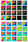 |
Fig. 4 Zoomof the spatial distribution of the integrated intensity (top) and peak temperature (bottom) towards the Horsehead nebula. |
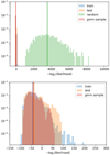 |
Fig. 5 Probability distribution function of the value of the Gaussian mixture fitted on the training set, for each data point. The log2-likelihood shown on the horizontal axis can be interpreted as the number of bits (to within a constant value) required to encode each point of the sample. The blue, orange, green, and pink colors show the distributions for the training set, the test set, a set of points uniformly drawn in the same multi-dimensional space, and a set of points randomly drawn in the Gaussian Mixture, respectively. The vertical lines show the associated means of the negative log2 -likelihood. Bottom panel: zoom of the top one. |
5.4 Optimization of the random forest regressor
Some algorithms have additional parameters, named hyper-parameters, which can be tuned to improve the quality of the regressor. In the case of random forests, the generalization performance can be optimized by tuning three hyper-parameters: (1) the maximum tree depth; (2) the fraction of features randomly chosen to train each node of each individual regression tree; and (3) the number of trees in the forest.
The values of these hyper-parameters are optimized to obtain the best generalization behavior of the predictor to previously unseen data. The goal is to have a predictor that is general enough to learn the complex non-linear relationship between observed features and the predicted quantity without learning the noise in the data set. The standard way of tuning the values of these hyper-parameters is to isolate a part of the training set as a validation set. We randomly put aside 4 out of 39 training rectangles as the validation set. The training procedure is repeated for different (fixed) values of the hyper-parameters. The best hyper-parameter values are then chosen as the ones that minimize the RMSE on the validation set. We also wish to maximize the amount of data used for training in case the validation set contains rare meaningful events (e.g., dense cores). To achieve this, random permutations of the validation sets are implemented and the hyper-parameters are chosen as the ones that are optimal over the average of the different validation sets. In our case, the best parameters are the ones that give the best average performance over ten such cross-validation draws.
We implemented a grid search to optimize these three hyper-parameters. Figure 6 shows the RMSE averaged over the ten cross-validation draws as a function of the three hyper-parameters as described in Sect. 5.2. The red cross shows the values of the hyper-parameters that minimize the RMSE: 300 for the number of trees, 32 for the tree maximum depth, and 30 randomly selected features (i.e., 75% of the total number of features). The optimization of the number of trees and maximum tree depth is particular because we expect that adding more trees monotonically increases the performance by reducing the variance. The most important piece of information here is that that the RMSE does not vary much when the number of trees is larger than 10, the maximum tree depth is larger than 16, and the fraction of randomly selected features is larger than 25%. This makes the overall random forest estimator robust to changes of these hyper-parameter values.
6 Comparison of the random forest prediction with two simpler methods
In order to show the power of the random forest predictor, we compare its performance with two other methods. We focus on the generalization performance of the predictors. This implies that we only check the prediction power on the test data set that has never been seen during the training phase.
 |
Fig. 6 Variations of the root mean square error (RMSE) between the predicted and the observed |
6.1 Multi-linear regression with or without a non-linear processing of the line intensities
Firstly, a standard ordinary least square method gives us the minimal achievable regression accuracy. We use the LinearRegression class from sklearn with the keyword normalize=True to apply a standard pre-whitening, that is, subtracting the mean and dividing by the standard deviation.
Secondly, we compare to the result obtained by Gratier et al. (2017). In this study, the linear principal component analysis (PCA) was preceded by the application of a asinh function to the original data set:
 (3)
(3)
where a is a constant cutoff. This non-linear transformation allowed us to take care of the specific properties of the histograms of the molecular emission. They are made of a Gaussian core around zero reflecting the noise properties and a power law tail that reflects the signal. The application of the asinh function had the double advantage of (i) applying a logarithm transform to the values above the asinh cutoff a to linearize the power law tail, while (ii) keeping the noise unchanged below the asinh cutoff a. This latter property allowed us to keep all the data set without noise clipping in the analysis. We use a common value of the asinh threshold a = 0.08 K or = 0.08 K km s−1 for the peak temperatures and integrated intensities, respectively, as in Gratier et al. (2017). After applying this transformation, we again use the LinearRegression class from sklearn with the keyword normalize=True as above.
6.2 Spatial distributions of the predictions and of the residuals
The first two columns of Fig. 7 show the spatial distribution of the observed and predicted column densities. The last column shows the ratios of the observed and predicted column densities for the three methods, on a logarithmic scale. It is thus equal to the difference between the logarithms of the predicted and observed column densities.
The residuals (right column of Fig. 7) indicate that all three regressions deliver column density predictions within a typical factor of two (i.e., ±0.3 dex). This means that it is indeed possible to predict the column density of the gas within a factor of two based only on the 3 mm line emission. However, the residuals between the predicted and observed values of  never look like random noise. This implies that the generalization of the column density predictor is imperfect in the three cases.
The comparison of the spatial distributions of the predicted column densities and the residuals for the three regression methods clearly shows that the linear regression is less successful than the other two non-linear methods. The left-right blue-red pattern indicates that the dense gas column density is clearly underestimated while the diffuse-translucent gas column density is overestimated for the linear predictor. The non-linear predictors perform better overall (lower contrast in the residuals).
The difference between the asinh pre-processing predictor and the random forest one is more subtle. The contrast of the residual image is slightly less pronounced for the random forest predictor. It does better than the asinh pre-processing in the dense cores, under the Horsehead muzzle, and in the diffuse-translucent gas above the Horsehead pillar. However, the back of the Horsehead (its mane) appears bluer in the residual maps of the random forest predictor.
6.3 Jointdistributions of the predicted and observed column density, and the histograms of their ratios
In order to quantitatively compare the three different methods, Fig. 8 shows the joint distributions of the predicted and observed column densities, as well as the histograms of their ratios. Table 3 lists the RMSE over the test set, the maximum root square error, as well as the mean of the ratios. These values here quantify the performance of the generalization of the method.
A linear regression gives a double-peaked histogram of the column density log-residuals (i.e., the base-10 logarithm of the ratio of the predicted over observed column density). This comes from the fact that the prediction overestimates the low column densities and underestimates the high column densities. The linear regression on the asinh of the intensities delivers a much better statistical agreement. Most of the predictions are close to the measured values even though there still is some scatter in particular at intermediate column densities. The joint histograms show that the asinh slightly underestimates the column density around 6.3 × 1021 cm−2 and slightly overestimates it above 1.6 × 1022 cm−2. The random forest predictor shows the least dispersion around the actual column density. All these properties translate into the fact that the histogram of the log-residuals is closest to a Gaussian for the random forest predictor.
These results are quantitatively confirmed by the values of the RMSE and the maximum absolute error listed in Table 3. The RMSE indicates that the predictors infer the column density within 20, 30, and 40% with a maximum error of a factor 1.8, 2.1, and 2.3, for the random forest, the asinh pre-processing, and the linear predictor, respectively. An additional piece of information is that all three methods over-estimate the column density by 20, 10, and 6% for the asinh pre-processing, the random forest and the linear predictors, respectively. This could be due to the fact that we tried to infer a positive quantity from noisy measurements where the centered noise sometimes hides the signal.
More quantitatively, we estimated the standard deviation on the mean error and MSE as
 (4)
(4)
where N is the number of pixels in the test set, and var is the variance of the error, that is, the difference between the logarithm of the predicted and observed values. The values listed in Table 3 shows that the difference between the mean errors associated with the random forest, and the asinh pre-processing methods is much larger than the sum of the associated standard deviations. A similar result is obtained for the mean square errors of the two methods. These two results mean that the random forest method yields a significantly better prediction than the asinh pre-processing.
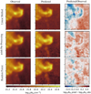 |
Fig. 7 Comparison of the generalization performances of three predictors. Top row: linear method. Middle row: linear method with a non-linear pre-processing. Bottom row: random forest. All results are computed on the Horsehead pillar, i.e., the test set. Left and middle columns: spatial distribution of the observed and predicted column density. Both images share the same color scale. Right column: ratio of the predicted column density over the observed one. The limits of the color scale correspond to a ratio interval from 1∕3 to 3. |
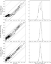 |
Fig. 8 Comparison of the generalization performances of three predictors. Top row: linear method. Middle row: linear method with a non-linear pre-processing. Bottom row: random forest. All results are computed on the Horsehead pillar, i.e., the test set. Left column: joint Probability Distribution Function (PDF) of the predicted column density and of the observed one. The contours are the PDF isocontours enclosing 25, 50, and 75% of the datapoints. Points whose density falls below these values are shown as black dots. The oblique lines have a slope of 1. They indicates ratio values of 1.0 (plain), 0.5 and 2.0 (dashed), 0.1 and 10.0 (dotted). Right column: histogram of the ratio of the predicted column density over the observed one on a logarithmic scale. The dotted lines show the Gaussian of same mean and width. |
6.4 Uncertainty
The fact that a random forest is an ensemble method can be leveraged to associate an uncertainty value to each predicted quantity. Atthe prediction step, the regression trees yield a set of 300 values and the mean of these values is the prediction of the random forest algorithm. It is thus possible to compute the value at a given percentile of the cumulative distribution of these 300 values. Specifically, we compute the values for the {2.3%, 15.9%, 84.1%, 97.7%} percentiles, which would correspond to 1 and 2σ uncertainty intervals for a Gaussian distribution.
Figure 9 compares the median prediction surrounded by the uncertainty intervals that comprise 68 and 95% of the trees with the column density of each pixel with the observed value. This confirms that column densities are well estimated between 2.5 × 1021 cm−2 and 1.6 × 1022 cm−2, and slightly over-estimated outside this interval. Nevertheless, the observed values are within the 95%–uncertainty interval for more than 90% of the test set.
The largest discrepancies between the observed and predicted values happen when the observed column density is lower than 2.5 × 1021 cm−2. In this range, the column densities are most often over-predicted for the three methods tested in this section. This could be related to the fact that 12CO (1–0) is overluminous in the diffuse gas, as already observed by Liszt & Pety (2012). Indeed, diffuse gas is actually present around the Horsehead pillar in the second velocity component between 2 and 8 km s−1, as mentioned in Pety et al. (2017). This behavior may have not been properly learned due to the lack of a clean example in the training set.
Statistical comparison of the performances of three regression methods on the test set (the Horsehead pillar).
 |
Fig. 9 Median column density and quantile intervals for each pixel of the test set ordered by increasing observed column density. Theblue dots display the associated observed column densities. |
7 Contribution of the different lines to the performance of the predictor
In the previous section, we show that the random forest predictor is able to approximate the column density with a precision of 20% on data points that belong to the same parameter space as the training set. We now try to quantify the contribution of the different molecular lines to this result. This question can be answered on both the training and test sets, as they belong to similar distributions of the input observables and targeted physical quantity. The advantage of the training set is that it contains 40 times as many points. The advantage of the test set is that the spatial variations of the input and targeted variables show shapes that are easy to describe. We thus use the training set to obtain global trends and the test set to discuss finer trends.
7.1 Lines that contribute the most
A first interpretative tool is the quantification of the line importance, that is, how much each line contributes to the prediction of  . To do this, we first keep the value of the RMSE computed on the training set as a reference. We then randomly permute the values of the intensities for a given line, all other intensities remaining constant. We finally compute the RMSE on the prediction using this shuffled data set. The increase in RMSE is the importance associated with the line. This importance has the same unit as the predicted quantity and it measures how much the performance would be degraded when the species is replaced by a noise that keeps the shape of the probability distribution function. For each line of sight, we simultaneously shuffle the values of the peak intensities and of the integrated intensity values of a given molecular line to estimate the overall importance of this line. Moreover, we try to check whether all lines have a significant contribution. We thus added two random data sets as additional input features to check which lines bring in more information than plain noise. We used two different random data sets to check that the result is not biased by any given random drawing.
The top panel of Fig. 10 shows the line importance by decreasing value for our data set. We first see that all lines bring more information than plain noise. Second, the (J = 1−0) line of 13CO, 12CO, C 18 O, HCO+, HNC, N2 H+, CCH, and the (J = 2−1) line of 12 CS have the largest line importance. Shuffling the 13CO samples increases the RMSE by ~0.22 dex (i.e., a factor 1.65 multiplying the reference factor of 1.2). The least important of these eight lines still increases the RMSE by 0.01 dex (or a factor 1.02), when shuffling its samples. Shuffling the data of any other line increases the RMSE by less than 0.01 dex.
Another way of visualising this effect is to build predictors with an increasing number of lines ordered by decreasing feature importance. The bottom panel of Fig. 10 clearly shows that adding more than the four of the most important lines only marginally increases the overall performance of the prediction. In other words, it seems that only four lines (the J = 1−0 line of the three main CO isotopologues, and HCO+) can predict  almost as well as when all the lines are included. We refine this statement further in Sect. 7.3. Adding more than the first eight lines even seems to bring no added value. This also shows that the random forest method is rather insensitive to the presence of “noisy” data in the input features.
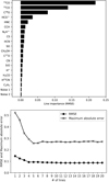 |
Fig. 10 Contribution of the different lines (both integrated intensity and temperature peak) to the quality of the random forest fit of the training data set. Noise #1 and 2 are two additional random sets of input data. Top: quantitative improvement of the quality of the fit (RMSE feature importance) for each available line. Bottom: evolution of the RMSE (filled circles) and maximum absolute error when each line is progressively added into the training phase in the order defined in the top panel. These results are computed on the training set. The RMSE values on each diagram are commensurate to log |
7.2 Where the lines contributes to the prediction
To confirm these quantitative measures, Fig. 11 shows the evolution of the spatial distribution of the predicted column density and of the associated residuals around the Horsehead pillar when building random forest predictors that are trained on an increasing number of lines ordered by their decreasing importance.
We see that the predictor trained only on the 13CO (1–0) line isable to recover the shape of the Horsehead pillar. This implies that this line contributes to differentiatethe column density between translucent and denser gas. Adding the contribution of the 12CO (1–0) line changes the residual maps mostly in the regions made of diffuse gas (red part on the right side). However, a predictor trained on these two lines alone provide a rather poor estimation of the column density in either the halo that surrounds the Horsehead pillar or the dense cores (e.g., the dense core at the top of the Horsehead or in its throat). Adding the C 18 O (1–0) line is important to improve the estimation within the denser parts (Horsehead spine and dense cores), while including the HCO+ (1–0) line improves the estimation of the column density in the far-UV-illuminated transition region between the translucent and denser gas. Completing the line sample with the HNC and N2 H+ (1–0) lines slightly changes the contrasts of the predicted images but this seems a second-order effect as the shape of the residuals does not change much when adding these lines. The most important change comes from the contribution of the N2 H+ (1–0) line tothe dense cores inside the Horsehead pillar.
Looking at the structure of regression trees, and random forests, it is possible to compute the contribution of each line, l, to the H2 column density. Indeed, it is possible to show3 that the predicted value of the column density at pixel (i, j) can be written as
 (5)
(5)
where logN0 is the mean of the column density over the training data set, and logNl is the quantitative contribution of each line (either integrated line profile or peak temperature) to the predicted value of the column density at pixel (i, j). Figure 12 shows the spatial distribution of the contribution of the eight lines most important to predict the column density. The first striking result is that all contribution maps show well-behaved structures (with extremely few exceptions), even though all lines are not detected over the full field of view. This suggests again that the column density estimate is rather insensitive to noise.
The contribution maps also allow us to quantitatively refine the scenario above. They confirm that the 13CO, 12CO, C 18 O, and HCO+ (1–0) lines are the first-order corrections to the mean value of the column density. The integrated intensity of 13CO contributes the most to the predictor. Its contribution map shows that it is important over the whole area. It contributes positively where the column density is high and negatively in the most far-UV illuminated regions. This coincides with the visual impression that the contribution map recovers well the shape of the Horsehead pillar. This is expected because the 13CO line traces most of the gas without being too optically thick. The second biggest contributor is the 12CO (1–0) line. It also contributes positively where the gas is translucent (see e.g., the clumps south of the Horsehead pillar). It is almost neutral (white or light blue around the Horsehead) where the gas is diffuse and it contributes negatively (dark blue) where the H II region dominates. The overall visual impression is that the 12CO line is importantto predict the diffuse to translucent part of the column density along the line of sight. The next two main contributors are the HCO+ and C18O (1–0) lines. They contribute in two complementary physical regimes. The C 18 O line contributes mostly where the gas is dense with a positive contribution at the highest densities (Horsehead spine) and a negative contribution at lower densities (nose, mane, feet). Conversely, the HCO+ line contributes mostly on the photo-dissociation regions that surround more or less dense gas. The comparison of the contribution maps of the integrated intensity and peak temperature for these four lines shows that the integrated intensities contribute more to the estimation of the column density. The peak intensities provide second order corrections, sometimes of opposite signs (clearest on the C 18 O line contributions) to the prediction of  . This suggests that these two parameters indeed play different roles in the estimation of the column density.
The next four most important lines are the J = 1−0 lines of HNC, N2H+, CCH, and the J = 2−1 line of 12CS. HNC, and N2H+COntribute mostly on the densest parts of the Horsehead pillar, that is, the dense cores and their surroundings. A striking feature is that the HNC peak temperature contributes one of the most important corrections in the places where the gas is dense, while its integrated intensity does not play a role in the prediction. This property is probably related to the detection pattern of this line in Fig. 4, which shows that the spatial distribution of the peak temperature is more contrasted or structured than the integrated line emission for the HNC line. Indeed, its integrated intensity varies between about 1 and 3 K km s−1 (it appears mostly red) everywhere it is detected in the horsehead pillar, while its peak temperature varies from about 0.3 to 2 K (its color varies from green to white) on the same region. Another striking feature is that the N2 H+ (1–0) peak temperature contribution map is structured even in regions where this line is not obviously detected. This probably means that the random forest has learned that a correction is needed when the N2 H+ line stays undetected. Finally, the CCH (1–0) and 12CS (2–1) lines contribute smaller corrections in photo-dissociation regions and UV-shielded dense gas, respectively. The peak temperatureand integrated intensity of both lines contribute corrections of similar magnitude.
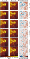 |
Fig. 11 Evolution of the prediction of the column density when adding molecular tracers one by one during the training phase. Left and middle columns: spatial distribution of the observed and predicted column densities. Both images share the same color scale. Right column: ratio of the predicted column density over the observed one. The limits of the color scale correspond to a ratio interval from 1∕5 to 5. |
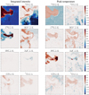 |
Fig. 12 Spatial distribution of the contribution of the integrated intensity and the peak temperature of the eight most important lines to the estimation of |
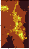 |
Fig. 13 Spatial distribution of the four following masks: 1 ≤ Av < 2 in black, 2 ≤ Av < 6 in brown, 6 ≤ Av < 15 in orange, and 15 ≤ Av in yellow. |
7.3 The physical regime each line contributes to
The line importance discussed in Sect. 7.1 is computed on the full training set that indifferently mixes all physical regimes. However, the contribution maps discussed in the previous section clearly showed that some lines are more important in certain particular physical regimes. We thus now ask whether some other lines are important for a given physical regime of column densities. Using the same categories as discussed in Pety et al. (2017), we compute the line importance on four subsets of the training set (see Fig. 13): 1 ≤ Av < 2 (diffuse gas: 14 377 pixels), 2 ≤ Av < 6 (translucent gas: 34 635 pixels), 6 ≤ Av < 15 (filaments: 8 723 pixels), and 15 ≤ Av (dense cores: 1 545 pixels). Figure 14 shows the line importance diagrams for the four different intervals of visual extinction.
The 13CO line is important for the estimation of the column density in all kinds of environments, except in dense cores. However, it is the most important only in the translucent gas. In diffuse gas, it contributes much less to the accuracy than the 12CO (1–0) line. In the filamentary gas, it contributes less than the C18O and HNC (1–0) lines. The 12CO (1–0) line isimportant in all regimes. However, while it completely dominates the estimation in diffuse gas, its importance regularly decreases when the visual extinction increases. The CCH (1–0) line plays a role in diffuse and translucent gas and almost no role in the two larger visual extinction regimes. The HCO+ (1–0) line plays an important role in diffuse and translucent gas (third line after the 12CO and 13CO (1–0) lines), and some role in relatively dense gas (6th line for filaments) when it is exposed to far-UV illumination. Its role is minor in the prediction for dense cores.
The C18O and HNC (1–0) lines play major roles in relatively dense gas, that is, among the filaments and dense cores. Finally, the N2 H+ and CH3OH lines are the most important ones to accurately predict the column density in dense cores where the CO isotopologues are depleted. This finding clearly indicates that line importance (as defined here) must be interpreted with caution when the populations of the different physical regimes are unbalanced in the training data set. A change in the RMSE value appears larger when a physical regime that is impacted is over-represented and vice-versa.
Figure 15 shows the contribution of the most important lines to the logarithm of the  column density as a function of the visual extinction. One red point per pixel of the test set is plotted. The black histograms show the median values of all data points falling in a regularly sampled interval of the logarithm of the visual extinction. As the test set does not contain many pixels at high visual extinction, the typical contribution of each line at Av ≳10 is not as well constrained as at lower visual extinction. The scatter around each typical value of the histogram comes from two sources. Tunings 2 and 3 are noisier than tuning 1 (see Table 1 for the list of relevant lines). However, noise does not explain all the observed scatter. A large fraction of the scatter comes from the fact that the combined measurement of several lines is indeed required to yield an accurate value of the column density at any given Av.
For each line, the contribution is computed as the sum of the contribution of the line peak temperature and integrated intensity. These contributions have to be added to the mean logarithm of the column density computed over the training set to get the column density value of the considered pixel of the test set. A contribution value of zero implies that the line has no impact at the associated visual extinction. This is clearly the case of the noise feature. A value of −0.2 or 0.2 implies that the line intensities require to multiply the column density by 0.63 or 1.58, respectively. This is the case of the 13CO (1–0) line that requires to multiply the average column density by a factor ~ 0.6 below Av ~ 5 and by a factor ~1.6 above Av ~ 10. Except for the 13CO (1–0) line that contributes at every Av and the noise sample that does not contribute at any Av, the other lines contribute inside a given Av range. The lines are sorted from top to bottom and then from left to right by increasing values of the minimum Av at which they start to contribute. The 12CO (1–0) line contributes at Av≲5, HCO+ (1–0) line in the range of 1≲Av≲10. The C 18 O and HNC (1–0) lines contribute at Av≳5, while the N2H+ (1–0) and CH3OH (2–1) lines start to contribute at Av≳10 and contribute even more at Av≳18.
 |
Fig. 14 Contributions of the different lines (both integrated intensity and temperature peak) to the quality of the |
 |
Fig. 15 Contribution of the most important lines to the logarithm of the H2 column density around the mean column density of the training set as a function of the visual extinction. One red points per pixel of the test set is plotted. The black histograms show the median values of all data points falling in a regularly sampled interval of the logarithm of the visual extinction. The black error bars show the range of values where 50% of the points in the current bin are located. The vertical dotted lines show visual extinctions of 1.1, 2.2., 5.0, 10.0, and 18.0. Except the 13CO (1–0) line that contributes at all Av and the noise sample that does not contribute at any Av, the other lines contribute inside a given Av range. The lines are sorted from top to bottom and then from left to right by increasing values of the minimum Av at which they start to contribute. |
7.4 Comparison with previous works on the Orion B molecular cloud
The results of this analysis shed a new light on the role of the molecular lines in tracing different gas density regimes in previous studies of the Orion B molecular cloud.
The main lines contributing to an accurate estimation of the H2 column density – the J = 1−0 lines of 12CO, 13CO, C 18 O, and HCO+ – had already been identified as effective tracers of the density regime by Bron et al. (2018). In particular, the three main CO isotopologues trace the transition from diffuse (~102 cm−3) to relatively dense (~103 cm−3) gas well, with an increasing importance of the rarer isotopologues at higher densities. Bron et al. (2018) also showed that adding the HCO+ (1–0) line brings sensitivity (1) to higher density regions (up to ~105 cm−3); and (2) to far-UV illuminated regimes in the regions of lower densities (≤ 103 cm−3). While the latter result is confirmed by this study, the former result, that is, the role of HCO+ in detecting regions of higher densities is in opposition to the random forest results, where this tracer only plays a minor role in the dense medium. This probably comes from the methodological differences between the two studies. Firstly, Bron et al. (2018) used a discrete clustering approach, while we use a continuous method here. Secondly, Bron et al. (2018) only used a subset of the lines studied here.
The qualitative study of the correlation between molecular line intensities and column densities performed by Pety et al. (2017) also contains results that are quantitatively confirmed by the current analysis. The 13CO (1–0) and C 18 O (1–0) lines were already identified overall as good tracers of the H2 column density, meaning that they have a monotonous relationship with low scatter over a broad range of column densities. The contribution of the different molecular lines to the random forest estimator of the column density in various extinction regimes (see Fig. 14) is consistent with the earlier results from Pety et al. (2017). In particular, the HCO+ (1–0) line is confirmed to contribute at low extinctions, despite its high critical density, while the actual best tracers of dense gas are the N2 H+ (1–0) and CH3OH (2–1) lines. This latter point was already observed by Gratier et al. (2017), who noted the strong anti-correlation of these lines with the emission of CO isotopologues in dense gas where CO depletion occurs. The role of the CCH (1–0) as a tracer of diffuse, far-UV illuminated regions was noted by Pety et al. (2017); Gratier et al. (2017); Bron et al. (2018), and by earlier studies of the Horsehead photo-dissociation region (e.g., Pety et al. 2005, 2012; Pilleri et al. 2013; Guzmán et al. 2015).
Previous studies of Orion B have also used a single molecular tracer as a simple proxy for the H2 column density, either for the bulk of the cloud (13CO J = 1−0 in Orkisz et al. 2017) or for the dense filaments and pillar regimes (C18O J = 1−0 in Hily-Blant et al. 2005; Orkisz et al. 2019). Figures 14 and 15 show that these qualitative choices of tracers are relatively well-suited for the targeted density regimes.
Statistical comparison of the performances with two simpler regression methods on the test set (the Horsehead pillar).
8 Comparison, generalization, limitations, and perspectives
In this section, we first discuss how random forest predictor of the column density we found compares with simpler approaches as the standard XCO-factor method. Wethen discuss how the found random forest predictor of the column density can be used on noisier or smoothed data sets. We also try to generalize the method to predict the far-UV illumination and discuss the fact that other physical variables partly control the 3 mm line strengths. Finally, we propose additional sources of information that could help to better constrain the physical conditions inside a giant molecular cloud.
8.1 Comparison with simpler approaches to infer the H2 column density from molecular lines
As explained in Sect. 3, the three main CO isotopologues are often used to derive the H2 column density because they are among the easiest detectable molecular lines in molecular clouds. Figures 16 and 17 show the performance to predict  of two simpler approaches. We first use the standard XCO-factor method, that is:

Secondly, we trained a random forest predictor using only (1–0) lines of the three main CO isotopologues, that is, 12CO, 13CO, and C 18 O. Table 4 lists the maximum error, mean error, and RMSE for these two methods and the random forest trained on all lines used in this article.
The XCO-factor method overall yields a poor inference of the column density in the Horsehead pillar. This behavior is well-known: the XCO-factor method only brings reasonable results when considering large fractions of a giant molecular cloud. By fitting the value of the XCO factor, we could, in principle, improve the mean error of the method on the test set but the large dispersion of the results would remain identical. A random forest trained on the three main CO isotopologues yields a much better inference of the column density. Its mean error is even lower than the random forest trained on all our lines. This implies that the simpler method is less biased but the histogram of the difference between the logarithms of the predicted and observed column densities is not centred on zero. This means that the predicted values are more often either under or over-estimated. This also implies a significantly larger RMSE. Lines such as the (1–0) lines of HCO+, CCH, HNC, and N2H+ are important for yielding more consistent results over the full range of visual extinction.
8.2 Noise and distance effects
Our training and test sets have been observed with a decent value for the S/N. We thus wonder whether it is possible to use the random forest prediction of the column density on observations that have low S/N To explore the predictive power of the method when confronted with noisy observations, we have computed the mean error and RMSE on the predicted column density when adding gradually increasing Gaussian noise to each channel of each spectra of the test set. The same noise rms value is used for all lines simultaneously.
The left panel of Fig. 18 shows the results of this procedure. The effect is negligible when the added noise RMS is lower than 0.1 K in channels of 0.5 km s−1. Both the mean error and the RMSE increase slowly for values of added noise between 0.1 and ~ 3 K. They then increase swiftly for larger noise values. These noise values have similar orders of magnitudes than the mean peak temperatures listed in Table 2. The mean peak temperatures belong to the [0.1, 0.5 K] interval for all lines except H40α that anyway plays a negligible role here, and the J = 1−0 line of 13CO and 12CO whose mean temperature are 3.4 and 14.0 K, respectively. This means that the detection of a given line is enough to make a first estimate of the H2 column density. This also implies that the column density predictor could be used on most observations taken today in millimeter astronomy as the ORION-B data set was obtained at the highest telescope velocity possible at the IRAM-30m telescope, that is, between 16 and 18″ s-1 (this limit coming from the data rate).
Our training and test sets also belong to one of the closest giant molecular clouds. We also consider the maximum distance at which it is still possible to use random forest prediction of the column density. We assume that our observations of other molecular clouds at larger distances from the Sun are made with the same telescope. This means that the linear resolution decreases with the distance, that is, the images of the input and predicted variables are consistently smoothed with increasing Gaussian kernels and then downsampled. The right panel of Fig. 18 shows the results. We conclude that it is possible to use the random forest predictor trained at the highest angular resolution up to a distance eight times as great while maintaining a similar level of precision. The predicted column density is then, of course, the beam-diluted column density.
8.3 Generalization to the prediction of the far-UV illumination
The far-UV illumination is another key parameter in the physics of molecular clouds. Thus, our next step is to check whether it is possible to quantitatively infer the far-UV illumination from the 3 mm molecular emission, that is, to check whether the procedure described above can be generalized to other physical quantities.
In far-UV illuminated regions, the dust emission is closely linked to the far-UV photon flux. Pety et al. (2017) converted the dust temperature map into an approximate map of the far-UV radiation field G0 in units of the Habing Interstellar Standard Radiation Field (ISRF, Habing 1968), using the simple approximation of Hollenbach et al. (1991) for face-on PDRs
 (8)
(8)
Shimajiri et al. (2017) compared this estimation with another estimation directly using the far-IR intensities at 70 and 100 μm. Both estimates agree within 30%. Given the complex geometry of molecular clouds with respect to the illuminating stars and the presence of far-UV shielded dust emission, the deduced values of G0 should only be trusted at order-of-magnitude levels. As for the observed column density used to train the random forest (see Sect. 2.2), we do not claim that our dust-traced estimation of the far-UV illumination is a perfect measure of G0. Another way of looking at this is to state that we only aim to predict the dust temperature from the 3 mm molecular emission alone here, as we try to predict log G0 that is linearly related to logTdust. However, our long-term goal is to infer the values of the parameters that control the underlying physics. That is why our main efforts are aimed at checking whether the 3 mm molecular emission alone is able to predict this dust-traced G0 with all its caveats (see also Sect. 8.5).
We used the same input features, the same training and test sets, and the same methods as those used to learn how to infer the H2 column density. Figure 19 shows the results. Quantitatively, the mean error on log G0 is 0.081 dex (i.e., a factor of 1.21), the RMSE is 0.25 dex (a factor of 1.8), and the maximum absolute error is 0.78 dex (a factor of 5.9). The prediction of the observed far-UV illumination is typically off by a multiplicative factor of 1.2 with a multiplicative scatter of 1.8 and errors of up to a factor of six. These values must be interpreted keeping in mind that the observed far-UV illumination around the Horsehead pillar spans slightly more than one order of magnitude. The joint distribution of the predicted and observed values of G0 shows a large scatter in the ranges 10−15 and 50−80. The histogram of the predicted over observed values shows a maximum around a factor 1.6, a secondary maximum around a factor 1.0, plus two other over-densities compared to a Gaussian of same mean and width at factors of 0.5 and 2.5. The comparison of the spatial distributions shows that the predicted G0 has variations that are much less smoothed than those of the observed G0, along with large errors in diffuse gas and dense photo-dissociation regions.
These results are not as good as for the column density. We interpret the lower quality prediction of G0 by the fact that the far-UV illumination is related to the third principal component in the work of Gratier et al. (2017). This only explains ~ 5% of the correlations present in the input data set, compared to 60% for the first principal component that is correlated to the column density. This means that G0 is more difficult to extract from the current set of line intensities detected in the 3 mm band. This set mainly contains one rotational transition per molecular species, most often the ground level one. It has been shown (see e.g., the companion paper Roueff et al. 2020) that these transitions probe the molecular column densities quite well, but that they are less efficient for constraining the excitation conditions of the species. It is expected that the sensitivity to G0 would be increased by adding information on the molecular excitation in warmer gas since the populations in higher energy levels are altered in regions illuminated by a high radiation field. This means that the line set should be complemented by higher level transitions of a subset of the species probed in the 3 mm band. This “excitation signature” will complement the “chemical signature” that is already present in the 3 mm line sample.
 |
Fig. 16 Performance of the standard XCO method to predict the column density from the 12CO (1–0) integrated line intensity. Top: spatial distribution of the observed and predicted H2 column density (left and middle panels), and of the ratio of the predicted column density over the observed one (right panel). Bottom: joint histogram of the predicted column density as a function of the observed one (left panel), and histogram of the ratio of the predicted column density over the observed one on a logarithmic scale. These results are computed on the Horsehead pillar, i.e., the test set. |
 |
Fig. 17 Performance of a random forest regression trained only on the three main CO isotopologues. The layout of the figure is identical to Fig. 16. |
 |
Fig. 18 Evolution of the accuracy (RMSE and mean error) of the |
8.4 Confounding variables
The intensity of a given line depends not only on the total column density of matter, but also on the molecule abundance, and the excitation conditions (kinetic temperature, density of neutrals, and electrons). The latter quantities, thus, can act as confounding variables in the relationship F between the total column density  and the input intensities Il. The lack of knowledge of these confounding variables implies that somewhat different values of the dust-traced column density are possible for a given set of line intensities, and thus acts as a source of uncertainty (of unknown distribution). In the absence of ancillary knowledge beyond the line intensities, the best estimation of the column density predictor nevertheless exists: It is the conditional expectation of the dust-traced column density, given the knowledge of the line brightnesses, mathematically ⟨
  |I1,..., IL⟩. In this paper, we ignore the effect of the confounding variables on the ground that the correlation between the line intensities in the PCA analysis are largely dominated by the first component which is, in turn, highly correlated with the column density. The presence of confounding variables induces a small additional uncertainty on the relationship between the dust-traced column density and the line intensities, which would need additional information to be lifted.
8.5 Other potential sources of information to improve the predictions of the gas column density and far-UV illumination
The dust-traced column density ( ) used in this article to train the random forest represents an approximate measure of the actual gas column density. Given the range of extinction, it is assumed that all gas is molecular and H I represents only a small fraction of the total gas column. Indeed, the column density of atomic-hydrogen-dominated gas (i.e., a very low molecular fraction) accounts for less than one visual magnitude of extinction in the studied field of view (Pety et al. 2017). A second assumption is the constancy of the dust-to-gas ratio over the whole region. Our study shows that the knowledge of the emission of a small number (six to eight) of 3 mm molecular lines is sufficient to predict the dust-traced column density in regions where the visual extinction is mostly associated with molecular gas.
In other regions, and especially when dealing with larger spatial scales, the dust thermal emission is associated with both atomic and molecular gas and is therefore used to determine the total gas column. At large scales (> 10 pc), and because the molecular gas is more concentrated than the atomic gas, the total gas column is often dominated by the contribution of atomic hydrogen. This applies to the large-scale halos around giant molecular clouds in our Galaxy as well as in external galaxies (e.g., Leroy et al. 2009). Remy et al. (2017, 2018b,a) shows that a fraction of the total gas column, called the CO-dark, remains unaccounted for when tracing the atomic gas with the H I 21 cm line and the molecular gas with the 12CO (1–0) emission using a simple linear method. The composition of the CO-dark gas (or more generally dark neutral medium) is actually a mixture of atomic gas when the 21 cm H I line becomes optically thick, and molecular gas with low CO abundance (e.g., Liszt et al. 2018, 2019). The regions dominated by H I or by the CO-dark gas have low to moderate extinctions. The emission in 12CO (1–0) is too weak in this gas to be easily detected at the sensitivity of typical observations.
While the random forest method is efficient for molecular cloud conditions as in those of Orion B, it will have to be tested in other regions to check how it behaves with regard to other data sets. Data sets covering a parameter space too far from that of ORION-B, as defined in Sect. 5.3, will have to be joined to the ORION-B data to generalize the training. When the physicalspace is, finally, correctly sampled, users should be able to apply the predictor. More generally, this method stillneeds to be anchored on more diverse data sets. These could be grids of models of photo-dissociation regions, which predict the line brightness of many species as a function of the column density for different physical regimes (Le Petit et al. 2006). Dust extinction maps derived from star counts (Capitanio et al. 2017) or from maps of the gamma ray fluxes (Remy et al. 2017, 2018b,a) would also provide independent estimates of the total column density, although at a lower spatial resolution than the molecular data. Finally, it would be interesting to complement the 3 mm molecular observations with velocity-resolved observations of the key H I 21 cm and 158 μm [C II] lines. Both lines would provide complementary information about the neutral gas not emitting in 12CO (1–0). As one of the strongest cooling lines, [C II] is also expected be a good probe of the far-UV illumination in combination with the 3 mm lines (Pabst et al. 2017, 2019).
 |
Fig. 19 Top: spatial distribution of the observed and predicted far-UV illumination (left and middle panels), and of the ratio of the predicted illumination over the observed one (right panel). Bottom: joint histogram of the predicted illuminationas a function of the observed one (left panel), and histogram of the ratio of the predicted illumination over the observed one on a logarithmic scale. These results are computed on the Horsehead pillar, i.e., the test set. |
9 Conclusions
In this paper, we show that it is possible to derive an estimator of the H2 column density from a set of molecular line observations. We used observations from the ORION-B data set to train the random forest on both the line integrated intensities and their peak temperatures. We obtained the following results.
-
When compared to linear regression on raw intensities or after a non-linear (asinh) processing of the intensities, the random forest regression delivers the best statistical agreement and thus provides the best generalization power. Indeed, the mean biases have a similar magnitude but the error variances and the maximum errors are the smallest for the random forest predictor.
-
On average, eight lines play the strongest role in the prediction of the H2 column density. The J = 1−0 lines of the three main CO isotopologues and HCO+ dominate the performance of the prediction. The J = 1−0 lines of HNC, N2H+, CCH, and the J = 2−1 line of 12CS make a contribution as second order corrections.
-
A deeper analysis shows that the 12CO (1–0) line is the most important line in diffuse gas (Av≲2), the 13CO (1–0) line in translucent gas (2≲Av≲5), the C18O (1–0) line in the filament gas (5≲Av≲15), and the N2H+ (1–0) and CH3OH(20 − 10) lines in dense cores (15 < Av).
-
The accuracy of the method over a large range of visual extinction depends on the number of lines measured. In particular, the intensity from a single line can not alone bring an accurate H2 column density under all the physical regimes, for example, when the gas is more far UV-illuminated or less.
-
The prediction of the far-UV illumination field using the same method is less successful, probably because the set of lines we use is not sensitive enough to the excitation conditions of the gas.
This work givesfurther support to the use of the CO isotopologues for deriving the total column density in molecular gas. It indicates that acquiring the three main isotopologues should be preferred over targeting a single CO line because they are sensitive to different ranges of visual extinction (e.g., diffuse, translucent, dark lines of sight). To further progress on the understanding of the physical conditions of molecular clouds, a detailed understanding of the variations of the CO isotopologue excitation conditions and relative abundances is needed. This will be the subject of further articles in this series, starting with a companion article by Roueff et al. (2020), which derives accurate excitation temperatures and column densities of the three main CO isotopologues.
Acknowledgements
This work is based on observations carried out under project numbers 019-13, 022-14, 145-14, 122-15, 018-16, and finally the large program number 124-16 with the IRAM 30 m telescope. IRAM is supported by INSU/CNRS (France), MPG (Germany) and IGN (Spain). This research also used data from the Herschel Gould Belt survey (HGBS) project (http://gouldbelt-herschel.cea.fr). The HGBS is a Herschel Key Programme jointly carried out by SPIRE Specialist Astronomy Group 3 (SAG 3), scientists of several institutes in the PACS Consortium (CEA Saclay, INAF-IFSI Rome and INAF-Arcetri, KU Leuven, MPIA Heidelberg), and scientists of the Herschel Science Center (HSC). We thank CIAS for their hospitality during the many workshops devoted to the ORION-B project. This work was supported in part by the Programme National “Physique et Chimie du Milieu Interstellaire” (PCMI) of CNRS/INSU with INC/INP, co-funded by CEA and CNES. This project has received financial support from the CNRS through the MITI interdisciplinary programs. J.R.G. thanks Spanish MICI for funding support under grant AYA2017-85111-P.
Appendix A: Interpreting the negative log2-likelihood of a set of points
If X is a discrete random variable whose probability distribution is pi = P(X = xi) with ∑ipi = 1, Q(X = xi) = −log2pi can be interpreted as the quantity of information associated to the event X = xi (see, e.g., Cover & Thomas 1991). For instance, having knowledge of an unlikely event corresponds to a large quantity of information.
Moreover, the quantity of information of a couple of independent events is simply the sum of both quantities. Indeed, Q(X = xi, Y = yj) = Q(X = Xi) + Q(Y = yj), because P(X = xi, Y = yj) = P(X = xi)P(Y = yj). For a source of information X, the statistical mean of Q(X) is
 (A.1)
(A.1)
According to Shannon coding theory, the quantity H(X) = −∑ipi log2pi, called the (Shannon) entropy, is equal to the number of bits required to encode the information. It thus allows one to quantify the quantity of information of a source X.
In practice, the distribution pi of X may be unknown, but we can postulate that the source X is described by another probability distribution qi. The expectation,
 (A.2)
(A.2)
is the number of bits necessary to encode the same source (i.e., X), but with q (which is known) instead of p (which is unknown). It is a straightforward path to showing that
 (A.3)
(A.3)
We thus yield
 (A.4)
(A.4)
where H(X) is the unknown entropy of the source (i.e., the number of bits necessary to encode the source X) and  is the Kullback-Leibler divergence. We can thenshow that
  . Thus, the entropy is the minimum amount of information required to encode the source, X, and the Kullback-Leibler divergence represents the number of bits that needs to be added when we encode the source X with q instead of p, that is, the cost (in bits) of choosing the wrong probability density, q.
When we quantify a continuous random variable X with resolution Δ to get a discrete random variable XΔ, we can show
 (A.5)
(A.5)
where
 (A.6)
(A.6)
is called thedifferential entropy. An important difference between entropy and differential entropy is that h(X) can be negative because of the logΔ offset. Nevertheless, the previous interpretation of the Kulback-Leibler divergence (i.e., the cost of choosing a different probability density instead of the actual one) remains valid up to a constant offset related to the quantification resolution. In others words, if we assume that there exists an unknown density fX of X, but we use the density g instead of f, we get
 (A.7)
(A.7)
where the Kullback-Leibler divergence  is always positive.
Figure 5 shows the histograms of the negative log2 -likelihood of the estimated Gaussian mixture for different data sets. It thus represents (within an unknown offset) the quantity of information that is necessary to encode the data sets with the Gaussian mixture model. The green histogram shows that the information cost is very high for a uniformly distributed random set, while it is similar for the training set and the test set.
References
- André, P., Men’shchikov, A., Bontemps, S., et al. 2010, A&A, 518, L102 [NASA ADS] [CrossRef] [EDP Sciences] [Google Scholar]
- Bachiller, R., & Cernicharo, J. 1986, A&A, 166, 283 [NASA ADS] [Google Scholar]
- Barnes, P. J., Hernandez, A. K., Muller, E., & Pitts, R. L. 2018, ApJ, 866, 19 [CrossRef] [Google Scholar]
- Bishop, C. M. 2006, Pattern Recognition and Machine Learning (Information Science and Statistics) (Berlin, Heidelberg: Springer-Verlag) [Google Scholar]
- Bolatto, A. D., Wolfire, M., & Leroy, A. K. 2013, ARA&A, 51, 207 [Google Scholar]
- Boucaud, A., Huertas-Company, M., Heneka, C., et al. 2020, MNRAS, 491, 2481 [NASA ADS] [CrossRef] [Google Scholar]
- Breiman, L. 2001, Mach. Learn., 45, 5 [CrossRef] [Google Scholar]
- Bron, E., Daudon, C., Pety, J., et al. 2018, A&A, 610, A12 [NASA ADS] [CrossRef] [EDP Sciences] [Google Scholar]
- Capitanio, L., Lallement, R., Vergely, J. L., Elyajouri, M., & Monreal-Ibero, A. 2017, A&A, 606, A65 [NASA ADS] [CrossRef] [EDP Sciences] [Google Scholar]
- Cernicharo, J., & Guelin, M. 1987, A&A, 176, 299 [NASA ADS] [Google Scholar]
- Clark, P. C., Glover, S. C. O., Ragan, S. E., & Duarte-Cabral, A. 2019, MNRAS, 486, 4622 [NASA ADS] [CrossRef] [Google Scholar]
- Cover, T. M., & Thomas, J. A. 1991, Elements of Information Theory (New York: Wiley-interscience), 144 [CrossRef] [Google Scholar]
- Dickman, R. L. 1978, ApJS, 37, 407 [NASA ADS] [CrossRef] [Google Scholar]
- Dickman, R. L., Snell, R. L., & Schloerb, F. P. 1986, ApJ, 309, 326 [NASA ADS] [CrossRef] [Google Scholar]
- Frerking, M. A., Langer, W. D., & Wilson, R. W. 1982, ApJ, 262, 590 [NASA ADS] [CrossRef] [Google Scholar]
- Fuente, A., Goicoechea, J. R., Pety, J., et al. 2017, ApJ, 851, L49 [NASA ADS] [CrossRef] [Google Scholar]
- Genzel, R., Tacconi, L. J., Combes, F., et al. 2012, ApJ, 746, 69 [Google Scholar]
- Gerin, M., Goicoechea, J. R., Pety, J., & Hily-Blant, P. 2009, A&A, 494, 977 [NASA ADS] [CrossRef] [EDP Sciences] [Google Scholar]
- Goicoechea, J. R., Pety, J., Gerin, M., et al. 2006, A&A, 456, 565 [NASA ADS] [CrossRef] [EDP Sciences] [Google Scholar]
- Goldsmith, P. F., Heyer, M., Narayanan, G., et al. 2008, ApJ, 680, 428 [NASA ADS] [CrossRef] [Google Scholar]
- Gratier, P., Pety, J., Guzmán, V., et al. 2013, A&A, 557, A101 [NASA ADS] [CrossRef] [EDP Sciences] [Google Scholar]
- Gratier, P., Majumdar, L., Ohishi, M., et al. 2016, ApJS, 225, 25 [NASA ADS] [CrossRef] [Google Scholar]
- Gratier, P., Bron, E., Gerin, M., et al. 2017, A&A, 599, A100 [NASA ADS] [CrossRef] [EDP Sciences] [Google Scholar]
- Guzmán, V., Pety, J., Goicoechea, J. R., Gerin, M., & Roueff, E. 2011, A&A, 534, A49 [NASA ADS] [CrossRef] [EDP Sciences] [Google Scholar]
- Guzmán, V., Pety, J., Gratier, P., et al. 2012, A&A, 543, L1 [NASA ADS] [CrossRef] [EDP Sciences] [Google Scholar]
- Guzmán, V. V., Pety, J., Goicoechea, J. R., et al. 2015, ApJ, 800, L33 [NASA ADS] [CrossRef] [Google Scholar]
- Habing, H. J. 1968, Bull. Astron. Inst. Netherlands, 19, 421 [Google Scholar]
- Hastie, T., Tibshirani, R., & Friedman, J. 2001, The Elements of Statistical Learning, Springer Series in Statistics (New York, NY: Springer New York Inc.) [Google Scholar]
- Hily-Blant, P., Teyssier, D., Philipp, S., & Güsten, R. 2005, A&A, 440, 909 [NASA ADS] [CrossRef] [EDP Sciences] [Google Scholar]
- Hollenbach, D. J., Takahashi, T., & Tielens, A. G. G. M. 1991, ApJ, 377, 192 [NASA ADS] [CrossRef] [Google Scholar]
- Le Petit, F., Nehmé, C., Le Bourlot, J., & Roueff, E. 2006, ApJS, 164, 506 [NASA ADS] [CrossRef] [EDP Sciences] [Google Scholar]
- Lefloch, B., Bachiller, R., Ceccarelli, C., et al. 2018, MNRAS, 477, 4792 [NASA ADS] [CrossRef] [Google Scholar]
- Leroy, A. K., Bolatto, A., Bot, C., et al. 2009, ApJ, 702, 352 [Google Scholar]
- Leroy, A. K., Bolatto, A., Gordon, K., et al. 2011, ApJ, 737, 12 [Google Scholar]
- Liszt, H. S., & Pety, J. 2012, A&A, 541, A58 [NASA ADS] [CrossRef] [EDP Sciences] [Google Scholar]
- Liszt, H., Gerin, M., & Grenier, I. 2018, A&A, 617, A54 [NASA ADS] [CrossRef] [EDP Sciences] [Google Scholar]
- Liszt, H., Gerin, M., & Grenier, I. 2019, A&A, 627, A95 [Google Scholar]
- Lombardi, M., Bouy, H., Alves, J., & Lada, C. J. 2014, A&A, 566, A45 [NASA ADS] [CrossRef] [EDP Sciences] [Google Scholar]
- Menten, K. M., Reid, M. J., Forbrich, J., & Brunthaler, A. 2007, A&A, 474, 515 [NASA ADS] [CrossRef] [EDP Sciences] [Google Scholar]
- Molinari, S., Schisano, E., Elia, D., et al. 2016, A&A, 591, A149 [NASA ADS] [CrossRef] [EDP Sciences] [Google Scholar]
- Orkisz, J. H., Pety, J., Gerin, M., et al. 2017, A&A, 599, A99 [NASA ADS] [CrossRef] [EDP Sciences] [Google Scholar]
- Orkisz, J. H., Peretto, N., Pety, J., et al. 2019, A&A, 624, A113 [NASA ADS] [CrossRef] [EDP Sciences] [Google Scholar]
- Pabst, C. H. M., Goicoechea, J. R., Teyssier, D., et al. 2017, A&A, 606, A29 [NASA ADS] [CrossRef] [EDP Sciences] [Google Scholar]
- Pabst, C., Higgins, R., Goicoechea, J. R., et al. 2019, Nature, 565, 618 [NASA ADS] [CrossRef] [Google Scholar]
- Pagani, L., Lefèvre, C., Juvela, M., Pelkonen, V. M., & Schuller, F. 2015, A&A, 574, L5 [NASA ADS] [CrossRef] [EDP Sciences] [Google Scholar]
- Pedregosa, F., Varoquaux, G., Gramfort, A., et al. 2011, J. Mach. Learn. Res., 12, 2825 [Google Scholar]
- Pety, J. 1999, PhD thesis, Paris 6 University, France [Google Scholar]
- Pety, J., Gratier, P., Guzmán, V., et al. 2012, A&A, 548, A68 [NASA ADS] [CrossRef] [EDP Sciences] [Google Scholar]
- Pety, J., Teyssier, D., Fossé, D., et al. 2005, A&A, 435, 885 [NASA ADS] [CrossRef] [EDP Sciences] [Google Scholar]
- Pety, J., Guzmán, V. V., Orkisz, J. H., et al. 2017, A&A, 599, A98 [NASA ADS] [CrossRef] [EDP Sciences] [Google Scholar]
- Pilleri, P., Treviño-Morales, S., Fuente, A., et al. 2013, A&A, 554, A87 [NASA ADS] [CrossRef] [EDP Sciences] [Google Scholar]
- Pineda, J. L., Goldsmith, P. F., Chapman, N., et al. 2010, ApJ, 721, 686 [NASA ADS] [CrossRef] [Google Scholar]
- Planck Collaboration I. 2011, A&A, 536, A1 [NASA ADS] [CrossRef] [EDP Sciences] [Google Scholar]
- Remy, Q., Grenier, I. A., Marshall, D. J., & Casand jian, J. M. 2017, A&A, 601, A78 [NASA ADS] [CrossRef] [EDP Sciences] [Google Scholar]
- Remy, Q., Grenier, I. A., Marshall, D. J., & Casand jian, J. M. 2018a, A&A, 616, A71 [NASA ADS] [CrossRef] [EDP Sciences] [Google Scholar]
- Remy, Q., Grenier, I. A., Marshall, D. J., & Casand jian, J. M. 2018b, A&A, 611, A51 [NASA ADS] [CrossRef] [EDP Sciences] [Google Scholar]
- Ripple, F., Heyer, M. H., Gutermuth, R., Snell, R. L., & Brunt, C. M. 2013, MNRAS, 431, 1296 [NASA ADS] [CrossRef] [Google Scholar]
- Roueff, A., Gerin, M., Gratier, P., et al. 2020, A&A, 645, A26 [Google Scholar]
- Schneider, N., André, P., Könyves, V., et al. 2013, ApJ, 766, L17 [NASA ADS] [CrossRef] [Google Scholar]
- Shimajiri, Y., André, P., Braine, J., et al. 2017, A&A, 604, A74 [NASA ADS] [CrossRef] [EDP Sciences] [Google Scholar]
- Valdivia, V., Godard, B., Hennebelle, P., et al. 2017, A&A, 600, A114 [NASA ADS] [CrossRef] [EDP Sciences] [Google Scholar]
- Visser, R., van Dishoeck, E. F., & Black, J. H. 2009, A&A, 503, 323 [NASA ADS] [CrossRef] [EDP Sciences] [Google Scholar]
- Zucker, C., Speagle, J. S., Schlafly, E. F., et al. 2019, ApJ, 879, 125 [NASA ADS] [CrossRef] [Google Scholar]
- Zucker, C., Speagle, J. S., Schlafly, E. F., et al. 2020, A&A, 633, A51 [CrossRef] [EDP Sciences] [Google Scholar]
The data products associated with this article are available at https://www.iram.fr/~pety/ORION-B
A demonstration can be found at http://blog.datadive.net/interpreting-random-forests/
All Tables
Statistical comparison of the performances of three regression methods on the test set (the Horsehead pillar).
Statistical comparison of the performances with two simpler regression methods on the test set (the Horsehead pillar).
All Figures
 |
Fig. 1 Spatial distribution of the dust-traced H2 column density derived from Herschel data (André et al. 2010; Lombardi et al. 2014). The dotted grid is used to define the training and test sets. The white square in the bottom right around the Horsehead region corresponds to the test set where the random forest predictions will be compared to the observations. This subset is never used during the training phase. Only the remainder of the map is used as the training set. |
| In the text | |
 |
Fig. 2 Spatial distribution of the line integrated intensity for some of the detected lines in the 3 mm band, plus the dust-traced far-UV illumination (bottom left panel) and the dust-traced H2 column density (top right corner). The color-scales are logarithmic to reveal the distribution of faint signal and positive noise. The maps are rotated counter-clockwise by 14 degrees from the RA/Dec J2000 reference frame. The spatial offsets are given in arcsecond from the projection center located at |
| In the text | |
 |
Fig. 3 Spatial distribution of the line peak temperature for some of the detected lines in the 3 mm band, plus the dust-traced far-UV illumination (bottom left panel) and the dust-traced H2 column density (top right corner). The color-scales are logarithmic to reveal the distribution of faint signal and positive noise. The maps are rotated counter-clockwise by 14 degrees from the RA/Dec J2000 reference frame. The spatial offsets are given in arcsecond from the projection center located at |
| In the text | |
 |
Fig. 4 Zoomof the spatial distribution of the integrated intensity (top) and peak temperature (bottom) towards the Horsehead nebula. |
| In the text | |
 |
Fig. 5 Probability distribution function of the value of the Gaussian mixture fitted on the training set, for each data point. The log2-likelihood shown on the horizontal axis can be interpreted as the number of bits (to within a constant value) required to encode each point of the sample. The blue, orange, green, and pink colors show the distributions for the training set, the test set, a set of points uniformly drawn in the same multi-dimensional space, and a set of points randomly drawn in the Gaussian Mixture, respectively. The vertical lines show the associated means of the negative log2 -likelihood. Bottom panel: zoom of the top one. |
| In the text | |
 |
Fig. 6 Variations of the root mean square error (RMSE) between the predicted and the observed |
| In the text | |
 |
Fig. 7 Comparison of the generalization performances of three predictors. Top row: linear method. Middle row: linear method with a non-linear pre-processing. Bottom row: random forest. All results are computed on the Horsehead pillar, i.e., the test set. Left and middle columns: spatial distribution of the observed and predicted column density. Both images share the same color scale. Right column: ratio of the predicted column density over the observed one. The limits of the color scale correspond to a ratio interval from 1∕3 to 3. |
| In the text | |
 |
Fig. 8 Comparison of the generalization performances of three predictors. Top row: linear method. Middle row: linear method with a non-linear pre-processing. Bottom row: random forest. All results are computed on the Horsehead pillar, i.e., the test set. Left column: joint Probability Distribution Function (PDF) of the predicted column density and of the observed one. The contours are the PDF isocontours enclosing 25, 50, and 75% of the datapoints. Points whose density falls below these values are shown as black dots. The oblique lines have a slope of 1. They indicates ratio values of 1.0 (plain), 0.5 and 2.0 (dashed), 0.1 and 10.0 (dotted). Right column: histogram of the ratio of the predicted column density over the observed one on a logarithmic scale. The dotted lines show the Gaussian of same mean and width. |
| In the text | |
 |
Fig. 9 Median column density and quantile intervals for each pixel of the test set ordered by increasing observed column density. Theblue dots display the associated observed column densities. |
| In the text | |
 |
Fig. 10 Contribution of the different lines (both integrated intensity and temperature peak) to the quality of the random forest fit of the training data set. Noise #1 and 2 are two additional random sets of input data. Top: quantitative improvement of the quality of the fit (RMSE feature importance) for each available line. Bottom: evolution of the RMSE (filled circles) and maximum absolute error when each line is progressively added into the training phase in the order defined in the top panel. These results are computed on the training set. The RMSE values on each diagram are commensurate to log |
| In the text | |
 |
Fig. 11 Evolution of the prediction of the column density when adding molecular tracers one by one during the training phase. Left and middle columns: spatial distribution of the observed and predicted column densities. Both images share the same color scale. Right column: ratio of the predicted column density over the observed one. The limits of the color scale correspond to a ratio interval from 1∕5 to 5. |
| In the text | |
 |
Fig. 12 Spatial distribution of the contribution of the integrated intensity and the peak temperature of the eight most important lines to the estimation of |
| In the text | |
 |
Fig. 13 Spatial distribution of the four following masks: 1 ≤ Av < 2 in black, 2 ≤ Av < 6 in brown, 6 ≤ Av < 15 in orange, and 15 ≤ Av in yellow. |
| In the text | |
 |
Fig. 14 Contributions of the different lines (both integrated intensity and temperature peak) to the quality of the |
| In the text | |
 |
Fig. 15 Contribution of the most important lines to the logarithm of the H2 column density around the mean column density of the training set as a function of the visual extinction. One red points per pixel of the test set is plotted. The black histograms show the median values of all data points falling in a regularly sampled interval of the logarithm of the visual extinction. The black error bars show the range of values where 50% of the points in the current bin are located. The vertical dotted lines show visual extinctions of 1.1, 2.2., 5.0, 10.0, and 18.0. Except the 13CO (1–0) line that contributes at all Av and the noise sample that does not contribute at any Av, the other lines contribute inside a given Av range. The lines are sorted from top to bottom and then from left to right by increasing values of the minimum Av at which they start to contribute. |
| In the text | |
 |
Fig. 16 Performance of the standard XCO method to predict the column density from the 12CO (1–0) integrated line intensity. Top: spatial distribution of the observed and predicted H2 column density (left and middle panels), and of the ratio of the predicted column density over the observed one (right panel). Bottom: joint histogram of the predicted column density as a function of the observed one (left panel), and histogram of the ratio of the predicted column density over the observed one on a logarithmic scale. These results are computed on the Horsehead pillar, i.e., the test set. |
| In the text | |
 |
Fig. 17 Performance of a random forest regression trained only on the three main CO isotopologues. The layout of the figure is identical to Fig. 16. |
| In the text | |
 |
Fig. 18 Evolution of the accuracy (RMSE and mean error) of the |
| In the text | |
 |
Fig. 19 Top: spatial distribution of the observed and predicted far-UV illumination (left and middle panels), and of the ratio of the predicted illumination over the observed one (right panel). Bottom: joint histogram of the predicted illuminationas a function of the observed one (left panel), and histogram of the ratio of the predicted illumination over the observed one on a logarithmic scale. These results are computed on the Horsehead pillar, i.e., the test set. |
| In the text | |
Current usage metrics show cumulative count of Article Views (full-text article views including HTML views, PDF and ePub downloads, according to the available data) and Abstracts Views on Vision4Press platform.
Data correspond to usage on the plateform after 2015. The current usage metrics is available 48-96 hours after online publication and is updated daily on week days.
Initial download of the metrics may take a while.


