| Issue |
A&A
Volume 644, December 2020
|
|
|---|---|---|
| Article Number | A151 | |
| Number of page(s) | 13 | |
| Section | Numerical methods and codes | |
| DOI | https://doi.org/10.1051/0004-6361/202039456 | |
| Published online | 14 December 2020 | |
LOC program for line radiative transfer
Department of Physics, PO Box 64, 00014 University of Helsinki, Finland
e-mail: This email address is being protected from spambots. You need JavaScript enabled to view it.
Received:
17
September
2020
Accepted:
29
October
2020
Abstract
Context. Radiative transfer (RT) modelling is part of many astrophysical simulations. It is used to make synthetic observations and to assist the analysis of observations. We concentrate on modelling the radio lines emitted by the interstellar medium. In connection with high-resolution models, this can be a significant computationally challenge.
Aims. Our aim is to provide a line RT program that makes good use of multi-core central processing units (CPUs) and graphics processing units (GPUs). Parallelisation is essential to speed up computations and to enable large modelling tasks with personal computers.
Methods. The program LOC is based on ray-tracing (i.e. not Monte Carlo) and uses standard accelerated lambda iteration methods for faster convergence. The program works on 1D and 3D grids. The 1D version makes use of symmetries to speed up the RT calculations. The 3D version works with octree grids, and to enable calculations with large models, is optimised for low memory usage.
Results. Tests show that LOC results agree with other RT codes to within ∼2%. This is typical of code-to-code differences, which are often related to different interpretations of the model set-up. LOC run times compare favourably especially with those of Monte Carlo codes. In 1D tests, LOC runs were faster by up to a factor ∼20 on a GPU than on a single CPU core. In spite of the complex path calculations, a speed-up of up to ∼10 was also observed for 3D models using octree discretisation. GPUs enable calculations of models with hundreds of millions of cells, as are encountered in the context of large-scale simulations of interstellar clouds.
Conclusions. LOC shows good performance and accuracy and is able to handle many RT modelling tasks on personal computers. It is written in Python, with only the computing-intensive parts implemented as compiled OpenCL kernels. It can therefore also a serve as a platform for further experimentation with alternative RT implementation details.
Key words: radiative transfer / ISM: clouds / ISM: kinematics and dynamics / ISM: lines and bands / ISM: molecules / line: formation
© ESO 2020
1. Introduction
Our knowledge of astronomical sources is mainly based on observations of the radiation that is produced, removed, or reprocessed by the sources. This applies both to continuum radiation and to spectral lines. The sensitivity to the local physical conditions and the velocity information available via the Doppler shifts makes spectral lines a particularly powerful tool. The interpretation of the observations is complicated by the fact that we can view the sources only from a single direction. In reality, the sources are three-dimensional objects with complex variations of density, temperature, chemical abundances, and velocities.
Radiative transfer (RT) models help us to understand the relations between the physical conditions in a source and the properties of the observed radiation. In forward modelling, the given initial conditions lead to a prediction of the observable radiation that is unique, apart from the numerical uncertainties of the calculations themselves. The main challenges are related to the large size of the models (in terms of the number of volume elements), which may call for simplified RT methods, especially when RT is coupled to the fluid dynamics simulations. The model size can also be a problem in the post-processing of simulations, especially when more detailed RT calculations are called for. As a result, supercomputer-level resources may again have to be resorted to.
In the inverse problem, when a physically plausible model for a given set of observations is searched for, the models are usually smaller. However, modern observations can cover a wide range of dynamical scales, thus setting corresponding requirements on the models. The main problems are connected with the large parameter space of possible models. It is difficult to find any model that matches the observations. Moreover, the fact that the problem is inherently ill-posed means that (within observational uncertainties) there may be many possible solutions for which the allowed parameter ranges need to be determined. Therefore the RT modelling of a set of observations (the inverse problem) can be just as time-consuming and computationally demanding as the post-processing of large-scale simulations (the forward problem). Because of this complexity, observations are still often analysed in terms of spherically symmetric models, although 2D and 3D modelling is becoming more common. This is not necessarily a problem forced upon us by the computational cost, but can serve as a useful regularisation of the complex problem.
A number of freely available RT programs are available, some of which were compared in van Zadelhoff et al. (2002) and Iliev et al. (2009), and new programs and new versions of established codes continue to appear (Olsen et al. 2018). Within interstellar medium (ISM) studies, the codes used in the modelling of radio spectral lines range from programs using a simple escape probability formalism, such as RADEX (van der Tak et al. 2007), via 1D-2D codes such as RATRAN (Hogerheijde & van der Tak 2000) or ART (Pavlyuchenkov & Shustov 2004), to programs using full 3D spatial discretisation, often in the form form of adaptive or hierarchical grids. As examples, MOLLIE (Keto & Rybicki 2010) uses Cartesian and nested grids, LIME (Brinch & Hogerheijde 2010) employs unstructured grids, ART3 (Li et al. 2020) uses octree grids, RADMC-3D (Dullemond et al. 2012) is based on patch-based and octree grids, and Magritte (De Ceuster et al. 2020) makes use of even more generic information about the cell locations. Programs are still often based on Monte Carlo simulations. In the list above, only MOLLIE and Magritte appear to use deterministic (non-random) ray-tracing. In 3D models and especially when some form of adaptive or hierarchical grids is used, it is essential for good performance that the RT scheme takes the spatial discretisation into account. Otherwise, information of the radiation field cannot be transmitted efficiently to every volume element. Cosmological simulations deal with analogous problems, and various ray-splitting schemes are used to couple cells with the radiation from discrete sources (Razoumov & Cardall 2005; Rijkhorst et al. 2006; Buntemeyer et al. 2016). This becomes more difficult in Monte Carlo methods when the sampling is random.
On modern computer systems, good parallelisation is essential. After all, even on a single computer, the hardware may be capable of running tens (in the case of central processing units, CPUs) or even thousands (in the case of graphics processing units, GPUs) of parallel threads. Some of the programs already combine local parallelisation (e.g. using OpenMP1) with parallelisation between computer nodes (typically using MPI2). In spite of the promise of theoretically very high floating-point performance of the GPUs, these are not yet common in RT calculations, and within RT, they are more common in other than spectral line calculations (Heymann & Siebenmorgen 2012; Malik et al. 2017; Hartley & Ricotti 2019; Juvela 2019). However, parallel calculations over hundreds or thousands of spectral channels should be particularly well suited for GPUs (De Ceuster et al. 2020).
We present LOC, a new suite of radiative transfer programs for modelling spectral lines in 1D and 3D geometries, using deterministic ray-tracing and accelerated lambda iterations (Rybicki & Hummer 1991). The generated rays closely follow the spatial discretisation, which is implemented using octrees. LOC is parallelised with OpenCL libraries3, making it possible to run the program on both CPUs and GPUs. LOC is intended to be used on desktop computers, with the goal of enabling the processing of even large models with up to hundreds of millions of volume elements. The program includes options for the handling of hyperfine structure lines. Experimental routines handle the general line overlap in the velocity space and the effects from continuum emission and absorption. These features are not discussed in the present paper, which concentrates on the performance of LOC in the basic scenarios, without the dust coupling. In the case of hyperfine spectra, LOC assumes a local thermal equilibirum (LTE) distribution between the hyperfine components.
The contents of the paper are the following. The implementation of the LOC program is described in Sect. 2 and its performance is examined in Sect. 3 in terms of the computational efficiency and the precision in selected benchmark problems. The technical details are discussed further in Appendix A. As a more practical example, we discuss in Sect. 3.3 molecular line emission computed for a large-scale simulation of the ISM. The results are compared with LTE predictions and synthetic dust continuum maps. We discuss the findings and present our conclusions in Sect. 4.
2. Implementation of the LOC program
Line transfer with OpenCL (LOC) is a line radiative transfer program that is based on the tracing of a predetermined set of rays through the model volume4. Unlike in Monte Carlo implementations, the sampling of the radiation field contains no stochastic components.
The calculations use long characteristics that start at the model boundary and extend uninterrupted through the model volume. The only exception are the rays that in the 3D models are created in refined regions; they are discussed in Sect. 2.2. The rays express the radiation field in terms of photons rather than intensity, an approach more typical for Monte Carlo methods. However, LOC uses a fixed set of rays, without any randomness, and therefore is not a Monte Carlo program. Each ray contains a vector of photon numbers that corresponds to a regular velocity discretisation of the spectral line profile (typically some hundreds of channels). When a ray first enters the model, it carries information of the background radiation field. This is expressed as the number of photons that enter the model within each spectral channel in one second. If the background has an intensity of  and there is one ray for a given surface area A and solid angle Ω, the number of photons per channel is
 (1)
(1)
where Δv is the channel width in velocity, h is the Planck constant, and c is the speed of light. The total number of photons coming from different directions is represented with a small number of actual ray directions (typically some tens in 3D models), but the total number of simulated photons is exact. The number of photons per ray depends on the number of ray directions (determining Ω) and the number of rays per direction (determining A). If the rays are equidistant in 3D space, A still varies depending on the angle between the ray direction and the local normal direction of the model surface. If the rays are not equidistant, this causes additional changes in A that are taken into account in the above calculation. Non-equidistant rays are already used for the 1D models (see Sect. 2.1).
As a ray passes through a cell, we count the number of resulting induced upward transitions Slu (from a lower level l to an upper level u) in the examined species. The photons that entered the cell from outside and the photons that were emitted within the cell must be taken into account,
![Mathematical equation: $$ \begin{aligned} S_{lu} = \frac{h \nu s}{4 \pi V} B_{lu} \phi (v) \left( n_{\nu ,0} \frac{1-e^{-\tau _{\nu }}}{\tau _{\nu }} + n_{u} A_{ul} V \phi (\nu ) \left[ 1- \frac{1-e^{-\tau _{\nu }}}{\tau _{\nu }} \right] \right), \end{aligned} $$](/articles/aa/full_html/2020/12/aa39456-20/aa39456-20-eq3.gif) (2)
(2)
(cf. Juvela 1997). Here s is the distance travelled across the cell, τ is the corresponding optical depth in a spectral channel, V is the cell volume, nν, 0 is the number of incoming photons, Aul is the Einstein coefficient for spontaneous emission, and ϕ(ν) is the line profile function. The total number of upward transitions is the sum over all spectral channels. The latter term within the parentheses represents the photons that cause new excitations in the cell where they are emitted. The number of photons within the ray changes similarly because of the absorptions and emissions. At the point where the ray leaves the cell, it is equal to
 (3)
(3)
In practical calculations, ϕ(ν) is replaced by the fraction of emitted photons per channel. Furthermore, in both Eqs. (2) and (3) we must take into account that each cell is traversed by a number of different rays. Each ray is therefore associated only with a fraction of emission events that is proportional to the length s. This can be calculated because the simulations are deterministic and the total length Σs is known.
Equation (2) results in estimates of the transition rates as an effective average over the cell volume, as sampled by the rays. It does not calculate intensities at discrete grid positions. This again recalls the way in which the radiation-matter interactions are typically handled in Monte Carlo RT programs.
The radiation field computation is alternated with the solution of the equilibrium equations that gives updated estimates of the level populations in each cell. There Slu is used directly in place of the normal rate of radiative excitations BluIν, where Blu is the Einstein coefficient. These two steps are iterated until the level populations converge to the required precision. The final state is saved, and spectral line maps are calculated for selected transitions by a final line-of-sight (LOS) integration through the model volume.
LOC is parallelised using OpenCL libraries. The program consists of the main program (written in Python) and a set of OpenCL kernels (written in the C language) that are used for the computationally expensive tasks. In OpenCL parlance, the main program runs on the “host” and the OpenCL kernels are run on the “device”, which could be either the same main computer as for the host (i.e. the kernel running on the CPU), a GPU, or another so-called accelerator device. The simultaneous use of several devices is in principle possible but is not yet implemented in LOC. Whether run on a CPU or a GPU, the goal is to fully utilise the computing hardware for parallel RT calculations. Parallelisation follows naturally from the parallel processing of the individual rays and the parallel solving of the equilibrium equations for different cells. In OpenCL, individual threads are called work items. A group of work items forms a work group that executes the same instructions (on different data) in lock-step. This sets some challenges for the load balancing between the threads, and synchronisation is possible only between the work items of the same work group. GPUs allow parallel execution with a large number of work groups, with even thousands of work items.
To speed up the convergence of the level populations for optically thick models, LOC uses accelerated lambda iterations (ALI). This is implemented in its simplest form, taking into account the self-coupling caused by photons that are absorbed in the cell where they were emitted (the so-called diagonal lambda operator). In practice, this is done by excluding the latter term in Eq. (2) and by scaling the Einstein Aul coefficients in the equilibrium equations with the photon escape probability. The use of ALI does not have a noticeable effect on the time it takes to process a given number of rays, but it requires additional storage, one floating point number per cell to store the escape probabilities. It is also possible to run LOC without ALI. LOC is optimised for low memory usage, especially because the amount of GPU memory can be limited. The main design decision resulting from this is that the RT calculations are executed one transition at a time. This reduces the memory requirements, but has some negative impact on the run times because the same ray-tracing is repeated for each transition separately.
The ray-tracing, including the calculation of the radiative interactions, is implemented as an OpenCL kernel function. Similarly, the solving of the equilibrium equations and the computation of the final spectral line maps are handled by separate kernels. For some kernel routines alternative versions are available, for instance, to handle corresponding calculations in the case of hyperfine structure lines. LOC consists of two host-side programs, one for 1D and one for 3D geometries. These are described below as far as required to understand their performance and limitations.
2.1. LOC in 1D
The 1D model is spherically symmetric and consists of co-centric shells with values for the volume density, kinetic temperature, amount of micro-turbulence, velocity along the radial direction, and fractional abundance of the species. It is not possible to include any rotation in the 1D models. The radiation field is integrated along a set of rays with different impact parameters. These are by default equidistant, but can be set according to a power law. This may be necessary if the innermost shells are very small compared to the model size and could not otherwise be sampled properly without a very large total number of rays. The distance that a ray travels through each shell is pre-calculated. This speeds up the ray-tracing kernel that is responsible for following the rays and counting the radiative interactions in the cells. The 1D version of LOC includes the options for the handling of hyperfine lines, with the LTE assumption or with the general line overlap, as well as the effects of additional continuum emission and absorption (cf. Keto & Rybicki 2010).
The 1D version of LOC processes each ray using a separate thread, or in OpenCL parlance, a separate work item. Even in detailed 1D models, only up to some hundreds of rays are needed. This suggests that 1D calculations will not make full use of GPU hardware, which might be able to provide many more hardware threads. Nevertheless, in practical tests, GPUs often outperformed CPUs by a factor of a few (Appendix A).
2.2. LOC in 3D
The spatial discretisation of the 3D LOC models is based on octree grids, which in principle include regular Cartesian grids as a special case. In practice, the Cartesian grid case is handled by a separate kernel, where the ray-tracing algorithm is simpler and each ray is processed by a single work item. On octree grids, the ray-tracing is more complex, and the computations on a given ray are shared between the work items of a work group. The directions of the rays are calculated based on Healpix pixelisation (Górski et al. 2005) to ensure uniform distribution over the unit sphere.
The 3D ray-tracing is based on two principles. First, for any given direction of the rays, the total length of the ray paths is the same in all cells, except for the dependence on the cell size. There is thus no random variation in the radiation field sampling. Second, we assume that we have no knowledge of the radiation field variations at scales below the local spatial discretisation. This simplifies the creation of new rays by avoiding interpolation. Especially when LOC is run on a GPU, it would be costly (in terms of additional computations and synchronisation overheads) to try to combine the information carried by different rays.
The calculations loop over the different ray directions. When a direction is selected, the vector component with the highest absolute value determines the main direction of ray propagation. This tells which side of the model is most perpendicular to the main direction and thus most illuminated by the radiation with the current ray direction. This side is referred to as the upstream side or border, both for the model and for the individual cells. One ray is started corresponding to each of the surface elements on the upstream border of the model. The step between the rays initially corresponds to the cell size at the root level of the grid hierarchy. In the following, the level of the hierarchy level L = 0 refers to the root grid, L = 1 to the first subdivision to eight sub-cells, an so forth. The initial number of concurrent rays is thus equal to the number of L = 0 surface elements on the upstream border. The exact position of the rays within its surface element is not important.
As rays are propagated through the model volume, they can enter regions with a higher or lower level of refinement. The grid of rays follows the grid of spatial discretisation. When a ray comes from a cell at level L to a cell C that has been split further to eight smaller level L + 1 cells, and when that ray enters on the upstream border of the cell C, new rays are added (cf. Fig. 1). The original ray enters one of the level L + 1 sub-cells of C, and three new rays are added, corresponding to the other level L + 1 sub-cells of C that share the same upstream border. All four upstream rays (the original ray included) are assigned one quarter of the photons of the original ray.
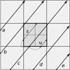 |
Fig. 1. Illustration of the creation of rays for a refined region. Rays a − e give a uniform sampling at the coarser level. Rays s and u are added for the refined region, using the information that ray c has of the radiation field at the upstream boundary of the refined cell. |
To keep the sampling of the radiation field uniform at all refinement levels, it may be necessary to add rays also on the other sides of the cell C that are perpendicular to the upstream border, two of which may also be illuminated by radiation from the current direction. A ray needs to be created if a ray corresponding to the discretisation level L + 1 would enter C through a neighbouring cell that itself is not refined to the level L + 1. If the neighbour is at some level L′< L, all the rays corresponding to the refinement at and below L′ will at some point exist in the neighbouring cell and will be automatically followed into cell C. These need not be explicitly created. However, the side-rays that correspond to discretisation levels above L′ and up to L + 1 have to be added, using the information from the original ray at the upstream border. If the step is ΔL = 1, the number of photons in the newly created ray is one quarter of the photons reaching the upstream cell boundary, as was the case for the new rays on the upstream border. This is not double counting because those photons should have entered cell C from a neighbouring cell, along a ray that did not exist because of the lower discretisation of the neighbouring cell. Unlike in the case of new rays on the upstream border, the need to add rays on the other sides has to be checked one every step, not only when the refinement changes along the original ray path.
The addition of the side-rays constitutes the longest extrapolation of the radiation field information: the ray entering the upstream side of C also provides part of the information for the radiation field at some other sides of C. Because side-rays are added only when the neighbouring cell is not refined to the level L + 1, the extrapolation is over a distance that corresponds to the spatial discretisation, that is, it is smaller than the size of the level L cells. For example, in most ISM models, there is structure at all scales, and if more accuracy is needed, it is usually better to improve the discretisation than to rely on higher-order interpolation of non-smooth functions.
Figure 1 illustrates the creation of new rays when the discretisation level increases by one. The main direction is upwards, and the thick arrows correspond to the rays on the coarser discretisation level. The central cell has been refined, and the shading indicates the extent of the refined region. When ray c enters the refined region, one new ray u is created on the upstream boundary based on ray c. In 3D, this would correspond to three new rays. This can be contrasted with Fig. 2 of Juvela & Padoan (2005), where the creation of a ray requires interpolation between three rays. Because in Fig. 1 the neighbouring cell on the left is less refined than the cells in the refined region, ray s has to be created at the boundary of the refined region. This is based on information from ray c. In Fig. 1, ray b also crosses the shaded refined cell. However, this ray already exists because the neighbouring cell on the left is refined to the same level as the central cell (before it was refined once). If the neighbouring cell had been even less refined, ray b would have been created as well. This would have taken place at the point where ray b enters the refined region and again only using information carried by ray c. In actual calculations, there are no guarantees on the order in which rays a-e are processed. However, rays s and u will be processed by the same work group as ray c. These rays will be followed until they again reach a coarser grid and are thus terminated, and the computation of ray c is resumed thereafter, at the point where it first entered the refined region. The order is important to reduce the required storage space (see below).
If the refinement level changes at a given cell boundary by more than ΔL = 1, the above procedure is repeated recursively. Each of the new rays is tagged with the hierarchy level at which it was first created, in the above example, level L + 1. When a ray reaches a region that is refined only to level L or lower, the ray is terminated. In theory, a better alternative would be to join the photons of the terminated sub-rays back to the ray(s) that continue into the less refined region. However, this would again require synchronisation and interpolation between rays that otherwise would not yet or would no longer exist (as they may be computed by other work groups, possibly during entirely different kernel calls). However, the termination of rays and thus the associated loss of information again only involves scales below the resolution of the local discretisation. When the refinement level decreases, the photon count of the rays that are not terminated is correspondingly scaled up by 4−ΔL, ΔL being the change in the refinement level (here a negative number).
When a ray exits the model volume through some side other than the downstream border, the corresponding work group (or, in the case of a Cartesian grid, a work item) creates a new ray on the opposite side of the model, at the same coordinate value along the main direction. The work group (work item) completes computations only when the downstream border of the entire model is reached. This also helps with the load balancing, although different rays may encounter different numbers of refined regions. With this ray-tracing scheme, each cell is traversed by at least by one ray per direction, and the physical path length is the same in all cells, except for the 0.5L dependence on the discretisation level.
One refinement requires the storage of three rays from the upstream border, the original level L ray, and two new rays that only exist at levels L + 1 and higher. The third of the new rays will be continued immediately. Four rays at most may be created at the other sides of cell C. When one ray is terminated, the next ray is taken from the buffer, unless this is already empty. To minimise the memory requirements, we always first simulate the rays created at higher refinement levels. The splitting of a ray requires storage of the ray locations and the single vector containing the original number of photons per velocity channel. Because the splitting is repeated for each increase in refinement level, one root-grid ray may lead to ∼7 × 3NL − 1 rays being stored in a buffer. This can become significant for large grids (e.g. a 5123 root grid, corresponding to 5122 simultaneous root-level rays). However, if necessary, the number of concurrent rays can be limited by simulating the root-grid rays in smaller batches.
The use of a regular grid of rays eliminates random errors in the sampling of the radiation field. The remaining numerical noise in the path lengths per cell in LOC is below 10−4 (tested up to six octree levels) and is thus mostly insignificant. While the path lengths are constant, the locations of the rays are not identical in all cells. This is part of the unavoidable sampling errors, but is again an error that is related to radiation field variations at scales below the spatial discretisation. The number of angular directions used in the calculations of this paper is 48.
The ray-tracing scheme used on octree grids, with the creation and termination of rays, is more complex than the simple tracing of individual rays through an octree hierarchy. Close to 90% of the code in the kernel for the radiation field simulation involves just the handling of the rays. As an alternative, it would be possible to use brute force and simulate a regular grid of rays with 4NL rays for every level L = 0 surface element. The simplified ray-tracing makes this competitive for grids with two levels, but it becomes impractical for deeper hierarchies because of the 4NL scaling.
3. Test cases
3.1. Tests with one-dimensional models
We tested the 1D LOC first using the Models 2a and 2b from van Zadelhoff et al. (2002). These are 1D models of a cloud core with infall motion, with 50 logarithmically divided shells, and with predictions computed for HCO+ lines. The two cases differ only regarding the HCO+ abundance, which is ten times higher in Model 2b. In this case, the optical depth was increased to τ ∼ 4800. van Zadelhoff et al. (2002) compared the results of eight radiative transfer codes. Figure 2 shows a reproduction. We overplot in the figure new computations with the Monte Carlo program Cppsimu (Juvela 1997) and the 1D version of LOC.
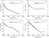 |
Fig. 2. Comparison of 1D LOC results for cloud models presented in van Zadelhoff et al. (2002). The plots show the radial excitation temperature profiles of the HCO+J = 1 − 0 and J = 4 − 3 transitions for Model 2a and the optically thicker Model 2b. The LOC results are plotted with hashed red lines, the results of the Monte Carlo code Cppsimu are shown in blue and the other results (van Zadelhoff et al. 2002) in black (with different line types). In frame d, the cyan line shows LOC results for an alternative interpretation of the problem set-up. |
The LOC results closely follow the average of the results reported in van Zadelhoff et al. (2002) as well as the recomputed Cppsimu Tex curve. Noticeable differences appear towards the centre of the optically thicker Model 2b, where LOC gives some of the lowest Tex values, although they are still within the spread of the 2002 results. The test problem was specified using a grid of 50 radial points. The results plotted in red were computed assuming that the grid points correspond to the outer radii of the shells and the listed physical values refer to the shells inside these radii. Especially in the inner part model, it also becomes important how the codes deal with the velocity field. In LOC, the Doppler shifts are only evaluated at the beginning of each step. Alternatively, the magnitude and direction of the velocity vector could be evaluated at the centre of the step, or even for several sub-steps separately. The LOC calculations used ∼100 velocity channels, the channel width being at most one fifth of the full width at half maximum (FWHM) of the local profile functions in the cells.
To illustrate the sensitivity of the results to the actual model set-up, we show in Fig. 2 results for an alternative LOC calculation. This uses the same discretisation as above (only splitting the innermost cell into two), but interpolates the input data to the radial distances that correspond to the average of the inner and outer radius of each cell. This results in changes that are of similar magnitude as the differences between the codes. The Tex values of the second LOC calculation even rise above the Cppsimu values. As noted in van Zadelhoff et al. (2002), better discretisation tends to decrease the differences between the codes. This reduces the effect of assumptions made at the level of the model discretisation and shows that the actual differences in the RT program implementations are only partly responsible for the scatter in the results.
3.2. Comparison of 1D and 3D models
To test the 3D version of LOC, we first compared it against 1D calculations made with Cppsimu and LOC. We adopted a spherically symmetric model with a radius of r = 0.1 pc, and the corresponding 3D models were discretised over a volume of 0.2 × 0.2 × 0.2 pc. The density distribution had a Gaussian shape with a centre density of n(H2) = 106 cm−3 and an FWHM of 0.05 pc. The model had a radially linearly increasing infall velocity (0–1 km s−1), kinetic temperature (10–20 K), turbulent linewidth (0.1–0.3 km s−1), and fractional abundance. The radial discretisation of the 1D model consisted of 101 shells, with the radii placed logarithmically between 10−4 and 0.1 pc. The 3D model extended further towards the corners of the cubic volume, but the hydrogen number density at the distance of 0.1 pc was already down to n(H2) ∼ 1.5 cm−3.
Figure 3 shows the results calculated for ammonia, including the hyperfine structure for the shown NH3(1, 1) lines and assuming an LTE distribution between the hyperfine components (Keto & Rybicki 2010). The fractional abundance was set to increase from 10−8 in the centre to 2 × 10⁻⁸ at the distance of 0.1 pc. Figure 3 shows the radial excitation temperature profiles and the spectra towards the centre of the model. In addition to the 1D calculations performed with Cppsimu and LOC, we show two sets of results from the 3D LOC. The first model used a regular Cartesian grid of 643 cells (with a size of 1.5625 mpc per cell), and the second added two levels of octree refinement, giving an effective resolution of 0.39 mpc. At each level, 15% of the densest cells of the previous hierarchy level were refined.
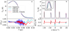 |
Fig. 3. Comparison of NH3(1, 1) excitation temperatures and spectra for a spherically symmetric cloud. Frame a shows the radial Tex profiles computed with 1D versions of the Cppsimu and LOC programs and with the 3D version of LOC. The LOC runs use either a Cartesian grid with 643 cells or the same with two additional levels of refinement. Frame b compares the spectra observed towards the centre of the model. A zoom into the peak of the main component is shown in the inset. The lower plots show the ratio of Tex values (frame a) and the difference between the LOC and Cppsimu TA values (frame b), with the colours listed in frame a. |
The excitation temperatures of the models match to within 5%. The largest differences result from the low spatial resolution of the pure Cartesian grid, combined with the regions of the steepest Tex gradients. The relative differences in Tex and absolute difference in TA are shown relative to the Cppsimu results, while the agreement between 1D and 3D LOC versions is slightly better. For the spectra, the residuals (up to ΔTA ∼ 0.2 K) are mainly caused by small differences in the velocity axis (a fraction of one channel, due to implementation details), while the peak TA values match to within 1%.
3.3. Large-scale ISM simulation
As an example of a more realistic RT modelling application, we computed molecular line emission from a large-scale magnetohydrodynamics (MHD) simulation of turbulent ISM. We used this to examine the convergence of the calculations in the case of a partially optically thick model, and to demonstrate the importance of non-LTE excitation.
3.3.1. Model setup
The model is based on the MHD simulations of supernova-driven turbulence that were discussed in Padoan et al. (2016) and were previously used in the testing of the continuum RT program SOC (Juvela 2019). The model covers a volume of (250 pc)3 with a mean density of n(H) = 5 cm−3.
We used LOC to calculate predictions for the 12CO(1–0) and 13CO(1–0) lines, using the molecular parameters from the Leiden Lamda database5 (Schöier et al. 2005). Because the used MHD run did not provide abundance information, we assumed for 12CO(1–0) abundances an ad hoc density dependence,
 (4)
(4)
This corresponds to the simulations of Glover et al. (2010). The fractional abundance of 13CO molecule was assumed to be lower by a factor of 50.
Because of the large volume, the model contains a wide range of velocities, but we included only a bandwidth of 50 km s−1 in the calculations. The higher velocities are exclusively associated with hot, low-density gas. With the assumed density dependence, the CO abundance of these regions is negligible.
We ran LOC on a system in which the host computer had only 16 GB of main memory. This required some optimisation to reduce the number of cells in the model. The original MHD data correspond to a root grid of 5123 cells and six levels of refinement. The total number of cells is 450 million. To reduce the memory footprint, we limited the RT model to the first three hierarchy levels and a maximum spatial resolution of 0.12 pc. However, because most cells are on the lower discretisation levels, this reduces the number of cells by only 22%, down to 350 million.
Because regions with low gas densities do not contribute significantly to the molecular line emission, we can further optimise by eliminating some of the refined cells. Whenever a cell was divided into sub-cells that all have a density below n(H2) = 20 cm−3, the refinement was omitted, replacing the eight sub-cells with a single cell. This is justified by the very low CO fractional abundance at this density (Eq. (4)). To increase the effect of this optimisation, the octree hierarchy was also first modified to have a root grid of 2563 cells and four instead of three refinement levels. By joining the low-density cells, the number of individual cells was reduced to 105 million, allowing the model to be run within the given stringent memory limits. The reduction in the number of cells also reduces the run times, which are approximately proportional to the number of individual cells (see Appendix A).
The kinetic temperature was left at a constant value of 15 K. The velocity dispersion in each cell was estimated from the velocities of the child cells (making use of the full model with seven hierarchy levels). The velocities were calculated similarly as density-weighted averages over the child cells. The number of velocity channels was set to 256, giving a resolution of 0.19 km s−1. This is comparable to the smallest velocity dispersion in individual cells (including thermal broadening). Ten energy levels were included in the calculations (the uppermost level J = 9 was about 300 K above the J = 0 level).
3.3.2. Convergence
The rate of convergence, and thus the number of required iterations, depends on the optical depths and will vary between regions. We are not affected by random fluctuations that in Monte Carlo methods would make it more challenging to track the convergence. Although 13CO can become optically thick in some of the densest clumps, convergence should be clearly slower for the main isotopic species. However, because of the strong inhomogeneity of the model, even the 12CO(1–0) line is optically thick only for some percent of the LOS, even though the maximum optical depth is close to τ = 100.
Figure 4 shows the change in 12CO(1–0) excitation temperature in different density bins and as a function of the number of iterations. The calculations start with LTE conditions, with excitation temperatures equal to the kinetic temperature, Tex ≡ Tkin = 15 K. The Tex values are seen to converge in just a few iterations. An accuracy of ∼0.01 K is reached last at intermediate densities, for n(H2) a few times 103 cm−3. This is because at higher densities the transition is thermalised and the Tex values remain close to the original value. There relation between volume density and excitation temperature is not unique. For a given volume density, the Tex values can vary by up to a few degrees, depending on the local environment, and they show more scatter above than below the main trend.
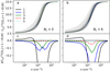 |
Fig. 4. Average 12CO(1–0) excitation temperatures in different density bins in the large-scale ISM simulation. The colours correspond to the situation after a given number of iterations, as indicated in the legend. The left frames show results for a model with a of 2563 cell root grid and NL = 3, and the right frame shows this for the same model with NL = 4. For a given density, the grey bands indicate the 1%-99% and 10%–90% intervals of the Tex values. The lower plots show the differences in the Tex values between iterations 1-5 and the seventh iteration (an approximation of the fully converged solution). The horizontal dashed black line corresponds to the ΔTex = 0 K level. |
We show in Fig. 4 the results for two different model discretisations with the number of octree levels NL = 3 or 4. The calculations are seen to converge slightly more slowly in the NL = 4 case. One factor is the ALI acceleration, which is effective for optically thick cells. When such a cell is split into sub-cells, some iterations are needed to find the equilibrium state. Appendix B shows results from additional convergence tests with the HCO+ and HCN molecules.
3.3.3. Statistics of synthetic maps
We examined some basic statistics of the synthetic maps. This was done in part to motivate the necessity for the time-consuming non-LTE calculations, instead of using more easily accessible quantities such as the model column density or the line emission calculated under the LTE assumption.
Figure 5 compares the computed line-area map W(13CO,J = 1 − 0) to the corresponding maps of the true column density and the surface brightness of the 250 μm dust emission. The dust emission is included as a common tracer of ISM mass that also typically provides a higher dynamical range. The details of the continuum calculations are given in Appendix C. Figure 5 shows that the 13CO emission is limited to the densest cloud regions, mainly because of the assumed density dependence of the fractional abundances. The colour scale of the W plot extends down to 10−5 K, although such low values are not detectable in any practical line surveys. The noisy appearance of the line area map is caused by abundance variations at small scales, although the variations in the line excitation have a secondary but still important role.
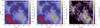 |
Fig. 5. Comparison of dust and line emission for a large-scale ISM simulation. The frames show the model column density (frame a), the computed 250 μm surface brightness of dust emission (frame b), and the13CO(1–0) line area (frame c). The white square in frame c indicates an area selected for closer inspection. |
The difference between the LTE and non-LTE emission is illustrated further in Fig. 6 for a selected small region. The size of the map pixels corresponds to the smallest cell size of this NL = 4 model, some 0.12 pc, and is thus smaller than can be easily discerned in the plot. Both calculations use the same model discretisation and 13CO abundances. In addition to the lower average level of the non-LTE emission, the ratio of non-LTE and LTE maps varies in a complex manner. In the histograms of Fig. 6d, the difference increases towards lower column densities. However, the non-LTE case has more pixels with very low emission, and its histogram peaks at densities far below the plotted range. In the more practically observable range of W(13CO)≳10−2 K, the probability density distributions (PDFs) are more similar. It is also noteworthy that the non-LTE predictions extend to higher intensities, although the average excitation temperature is far below the Tkin = 15 K value. This is caused by the higher optical depth of the J = 1 − 0 transition, when the higher excitation levels are less populated and the ratio of the J = 0 and J = 1 populations is higher.
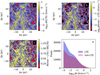 |
Fig. 6. Comparison of LTE (frame a) and non-LTE (frame b) predictions of W(13CO) for a region within the large-scale ISM simulation. The ratio of the LTE and non-LTE maps is shown in frame c. The corresponding histograms of W(13CO) values (above 10−3 K km s−1) are shown in frame d. The selected region is indicated in Fig. 5c with a white box. |
Figure 7 shows the dust and line emission plotted against the model column density. The dust emission shows good correlation, with only some saturation for the most optically thick LOS. In comparison, the scatter in the line intensities is large. For a given column density, the line area can vary by a significant factor, depending on the actual volume densities along the LOS. The large variation also applies to the column density threshold above which the line emission becomes detectable, N(H2) ∼ (2 − 17)×1021 cm−2. This scatter is again mainly due to the assumed abundance variations, although the non-LTE excitation also plays an important secondary role. Because of the ad hoc nature of the assumed abundances, Fig. 7 should be taken as a qualitative demonstration, not as a detailed prediction.
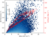 |
Fig. 7. Dust and 13CO line emission as functions of column density of the large-scale ISM simulation. The blue 2D histogram shows the distribution of the 13CO line area vs. the true column density. The colour bar indicates the number of pixels in the original line emission maps per 2D histogram bin. The corresponding distribution of 250 μm surface brightness vs. column density (right-hand axis) is shown with red contours. The contour levels correspond to log10npix = 0.5, 1, 2, and 3 for the number image pixels npix per 2D histogram bin. The number of 2D bins is the same as for the 250 μm surface brightness histogram. |
Figure 8 shows the power spectra calculated for different tracer maps. These include line area maps for constant and density-dependent abundances (Eq. (4)) for LTE conditions and the full non-LTE calculations with LOC. The power spectra were calculated with the TurbuStat package (Koch et al. 2019). The input maps have 2048 × 2048 pixels and a pixel size of 0.12 pc, which corresponds to the smallest cell size of the models (2563 root grid and NL = 4). The actual spatial resolution is lower over most of the map area, but the discretisation is identical for all the compared cases. The only exception is the 13CO map for the NL = 3 model, which is included as an example of a model with lower resolution.
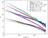 |
Fig. 8. Power spectra from synthetic observations of the large-scale ISM simulation. The power P is calculated for the true column density, the 250 μm dust surface brightness, and for three versions of 12CO line-area maps. The 12CO emission corresponds either to a constant abundance of χ0 = 10−4 and LTE conditions or to the Eq. (4) abundances with LTE or non-LTE calculations. The grey lines correspond to least-squares fits and extend over the range of the fitted spatial frequencies. |
The power spectra of the dust surface brightness map and the constant-abundance LTE map of 12CO line area are similar and even steeper than the spectrum of the true column density. With the density-dependent abundances, the power is increased at small scales. This results in much flatter power spectra. In the fits P ∼ kγ (k being the spatial frequency), the slope of the power spectrum rises above γ = −1.8. When the abundance distributions are identical, the 12CO power spectra are slightly flatter for the non-LTE than for the LTE case. The lower optical depth of the 13CO lines again increases the relative power at the smallest scales, resulting in the highest γ values. The difference between the NL = 3 and 4 discretisations has a smaller but still significant effect. The N = 3 cell size corresponds to a spatial scale outside the fitted range of k values, but the reduction of peak intensities (resulting from the averaging of cells in the N = 4 → 3 grid transformation) is reflected in all values of k.
4. Discussion and conclusions
The non-LTE, non-Monte-Carlo line transfer code LOC was shown to provide results in the selected 1D test problems (Sect. 3.1) that are comparable to those of other RT programs. The 3D version of LOC uses octree grids and is partly a separate code base. In the tests of Sect. 3.2, its results were consistent with the 1D version. The 3D program has also been compared with the Monte Carlo code Cppsimu (Juvela 1997) (not discussed in this paper), and those comparisons showed a similar degree of consistency. The differences in the results of different codes are also often connected with different interpretations of the model set-up rather than direct differences in the numerical methods themselves.
The parallelisation and the ability to run LOC on GPUs are important features. After all, even on desktop systems, the number of parallel threads provided by the hardware is approaching 102 on high end CPUs and 104 on high-end GPUs. Therefore, the lack of parallelisation or poor scaling to higher core counts would lead to unacceptable inefficiency in terms of the run times and the energy consumption. In the case of LOC, GPUs were found to provide a typical speed-up of 2–10 over a multi-core CPU (Appendix A), although the numbers vary depending on the actual model and the hardware used. The run times were found to be directly proportional to the number of transitions and the number of cells. In the case of very large models, the overhead from disc operations could decrease the performance, but this may be solved with more main memory. The run times appeared to be rather insensitive to the number of velocity channels, but this is at least partly due to the local emission or absorption profiles of the tested models, which cover only a small fraction of the computed bandwidth. When the number of channels is small, their effect on the run times is small because the effort spent on the basic ray-tracing is relatively large. When the number of channels is larger, the run time should depend linearly on it. There may also be some more discrete behaviour in details because on a GPU, a larger number of channels (e.g. 32) are processed in parallel. The number of channels should preferentially be a multiple of this local work group size (i.e. the group of threads with synchronous execution).
The example of Sect. 3.3 showed that relatively large models with up to hundreds of millions of cells can be handled on modest desktop computers and within a reasonable time. In Sect. 3.3, the original model was reduced to 105 million cells, and one RT iteration took less than three hours. With more memory, larger modelling tasks could be successfully attempted, such as the full model that contained 450 million cells (root grid 5123 and seven octree levels, see Sect. 3.3). This would still be within the reach of desktop computers, and with the most recent GPUs (compared to those used in the tests), the run times would still be of similar order. Conversely, RT calculations are also required in the case of small 1D models. When there are few observational constraints, simple 1D models are still a common aid in the interpretation of observations. Even much of the theoretical work still relies on 1D calculations, for example in the study of prestellar cores, where the spherical symmetry is a good approximation and the emphasis is on chemical studies (Vastel et al. 2018; Sipilä et al. 2019). Therefore both 1D and 3D RT programs are still relevant.
We showed in Sect. 3.3 that differences in the synthetic observations based on LTE and non-LTE calculations are clear even for the basic statistics, such as the power spectra and the intensity PDFs. In the ISM context, the non-LTE effects should be important for a wide range of numerical and observational studies of clouds and cores (Walch et al. 2015; Padoan et al. 2016; Smith et al. 2020), filaments, and velocity-coherent structures (Hacar et al. 2013, 2018; Arzoumanian et al. 2013; Heigl et al. 2020; Chen et al. 2020; Clarke et al. 2020), and the large-scale velocity fields (Burkhart et al. 2014; Hu et al. 2020). These problems are inherently 3D in nature, require the coverage of a large dynamical range, and are natural applications of line RT modelling on hierarchical grids. At the same time, RT is only one component of the problem and needs to be combined with descriptions of the gas dynamics and chemistry. For example, the sample calculations of Sect. 3.3 made use of a simple density dependence for the molecular abundances, but the real chemistry of the clouds and especially the transition between the atomic and molecular phases is more complex (Glover et al. 2010; Walch et al. 2015). Tools such as LOC are needed to quantify the observable consequences of different model assumptions and to ultimately test the models against real observations.
In the LOC results, the main errors are caused by the model discretisation and the sampling of the radiation field with a finite set of rays. The latter errors should decrease proportionally to ∼N−1, where N is the number of rays. This is significantly faster than the N−0.5 convergence of Monte Carlo methods, where on the other hand, the errors are explicitly visible as fluctuations between iterations. Some information of the sampling errors can be extracted also in LOC calculations, for example by using different ray angles. Changes in the spatial sampling are also possible but carry a high penalty because the number of rays per root-grid surface element has to be either one (the default value) or 4i, with i > 1. The noise in the level populations translates into errors in the predicted line profiles. The LOS integration tends to smooth out the errors. Nevertheless, the relative errors of the background-subtracted spectra (i.e. ON-OFF measurements) can again be higher if the lines are weaker than the background continuum.
The computational performance of LOC is still far from the theoretical peak performance, especially that of GPUs. The implementation of LOC as a Python program with on-the-fly compiled kernels is well suited for further development and testing of alternative schemes. When the device memory is not an issue, an obviously faster alternative for the 3D computations would be to process all transitions at the same time instead of repeating the ray-tracing for each transition separately. Because the rate of convergence is dependent on the local optical depths, some form of sub-iteration, where level populations are updated more frequently in optically thick regions, could result in significant reduction of the run times (cf. Lunttila & Juvela 2012). The number of energy levels that are actually populated varies significantly from cell to cell. This was true for the models discussed in Sect. 3.3, but would be much more evident if the models included strong temperature variations, for instance in the case of embedded radiation sources. Further optimisations would thus be thus possible by varying, cell by cell, the number of transitions for which RT computations are actually performed and the number of energy levels for which the level populations are stored.
LOC could also be extended with additional features. While it is possible to have several collisional partners with spatially variable abundances in the 1D models, the 3D version assumes their relative abundances to be constant (the abundance of the studied molecule itself is always specified for each cell separately). Continuum emission and absorption (e.g. from continuum RT modelling) cannot yet be considered in the 3D calculations. Similarly, while LOC can model lines with hyperfine structure, the general (non-LTE) case of line overlap is so far not included in the 3D version. Finally, if the spatial discretisation is coarse, there might be some advantage from the use of interpolated physical quantities. The use of velocity interpolation would require sub-stepping, each small step with a different Doppler shift. Therefore, further judicious refinement of the model grid might produce better results, even considering the run times.
The program documentation can be found at http://www.interstellarmedium.org/radiative_transfer/loc/, with a link to the source code at GitHub.
The 1D models were run on a six-core Intel i7-8700K CPU and NVidia GTX 1080 Ti GPU.
The CPU is a six-core Intel i7-8700K processor and the GPU an external Radeon VII card, connected via a Thunderbolt connection.
References
- Arzoumanian, D., André, P., Peretto, N., & Könyves, V. 2013, A&A, 553, A119 [NASA ADS] [CrossRef] [EDP Sciences] [Google Scholar]
- Brinch, C., & Hogerheijde, M. R. 2010, A&A, 523, A25 [NASA ADS] [CrossRef] [EDP Sciences] [Google Scholar]
- Buntemeyer, L., Banerjee, R., Peters, T., Klassen, M., & Pudritz, R. E. 2016, New A, 43, 49 [CrossRef] [Google Scholar]
- Burkhart, B., Lazarian, A., Leão, I. C., de Medeiros, J. R., & Esquivel, A. 2014, ApJ, 790, 130 [NASA ADS] [CrossRef] [Google Scholar]
- Chen, C.-Y., Mundy, L. G., Ostriker, E. C., Storm, S., & Dhabal, A. 2020, MNRAS, 494, 3675 [CrossRef] [Google Scholar]
- Clarke, S. D., Williams, G. M., & Walch, S. 2020, MNRAS, 497, 4390 [CrossRef] [Google Scholar]
- De Ceuster, F., Homan, W., Yates, J., et al. 2020, MNRAS, 492, 1812 [NASA ADS] [CrossRef] [Google Scholar]
- Dullemond, C. P., Juhasz, A., Pohl, A., et al. 2012, RADMC-3D: A Multi-purpose Radiative transfer Tool (Astrophysics Source Code Library) [Google Scholar]
- Fuente, A., Navarro, D. G., Caselli, P., et al. 2019, A&A, 624, A105 [NASA ADS] [CrossRef] [EDP Sciences] [Google Scholar]
- Glover, S. C. O., Federrath, C., Mac Low, M. M., & Klessen, R. S. 2010, MNRAS, 404, 2 [Google Scholar]
- Górski, K. M., Hivon, E., Banday, A. J., et al. 2005, ApJ, 622, 759 [NASA ADS] [CrossRef] [Google Scholar]
- Hacar, A., Tafalla, M., Kauffmann, J., & Kovács, A. 2013, A&A, 554, A55 [NASA ADS] [CrossRef] [EDP Sciences] [Google Scholar]
- Hacar, A., Tafalla, M., Forbrich, J., et al. 2018, A&A, 610, A77 [NASA ADS] [CrossRef] [EDP Sciences] [Google Scholar]
- Hartley, B., & Ricotti, M. 2019, MNRAS, 483, 1582 [CrossRef] [Google Scholar]
- Heigl, S., Gritschneder, M., & Burkert, A. 2020, MNRAS, 495, 758 [CrossRef] [Google Scholar]
- Heymann, F., & Siebenmorgen, R. 2012, ApJ, 751, 27 [NASA ADS] [CrossRef] [Google Scholar]
- Hogerheijde, M. R., & van der Tak, F. F. S. 2000, A&A, 362, 697 [NASA ADS] [Google Scholar]
- Hu, Y., Lazarian, A., & Yuen, K. H. 2020, ApJ, 897, 123 [CrossRef] [Google Scholar]
- Iliev, I. T., Whalen, D., Mellema, G., et al. 2009, MNRAS, 400, 1283 [NASA ADS] [CrossRef] [Google Scholar]
- Juvela, M. 1997, A&A, 322, 943 [NASA ADS] [Google Scholar]
- Juvela, M. 2019, A&A, 622, A79 [NASA ADS] [CrossRef] [EDP Sciences] [Google Scholar]
- Juvela, M., & Padoan, P. 2005, ApJ, 618, 744 [NASA ADS] [CrossRef] [Google Scholar]
- Keto, E., & Rybicki, G. 2010, ApJ, 716, 1315 [NASA ADS] [CrossRef] [Google Scholar]
- Koch, E. W., Rosolowsky, E. W., Boyden, R. D., et al. 2019, AJ, 158, 1 [CrossRef] [Google Scholar]
- Li, Y., Gu, M. F., Yajima, H., Zhu, Q., & Maji, M. 2020, MNRAS, 494, 1919 [CrossRef] [Google Scholar]
- Lunttila, T., & Juvela, M. 2012, A&A, 544, A52 [NASA ADS] [CrossRef] [EDP Sciences] [Google Scholar]
- Malik, M., Grosheintz, L., Mendonça, J. M., et al. 2017, AJ, 153, 56 [Google Scholar]
- Mathis, J. S., Mezger, P. G., & Panagia, N. 1983, A&A, 128, 212 [NASA ADS] [Google Scholar]
- Olsen, K., Pallottini, A., Wofford, A., et al. 2018, Galaxies, 6, 100 [NASA ADS] [CrossRef] [Google Scholar]
- Padoan, P., Juvela, M., Pan, L., Haugbølle, T., & Nordlund, Å. 2016, ApJ, 826, 140 [NASA ADS] [CrossRef] [Google Scholar]
- Pavlyuchenkov, Y. N., & Shustov, B. M. 2004, Astron. Rep., 48, 315 [NASA ADS] [CrossRef] [Google Scholar]
- Razoumov, A. O., & Cardall, C. Y. 2005, MNRAS, 362, 1413 [NASA ADS] [CrossRef] [Google Scholar]
- Rijkhorst, E. J., Plewa, T., Dubey, A., & Mellema, G. 2006, A&A, 452, 907 [NASA ADS] [CrossRef] [EDP Sciences] [Google Scholar]
- Rybicki, G. B., & Hummer, D. G. 1991, A&A, 245, 171 [NASA ADS] [Google Scholar]
- Schöier, F. L., van der Tak, F. F. S., van Dishoeck, E. F., & Black, J. H. 2005, A&A, 432, 369 [NASA ADS] [CrossRef] [EDP Sciences] [Google Scholar]
- Sipilä, O., Caselli, P., Redaelli, E., Juvela, M., & Bizzocchi, L. 2019, MNRAS, 487, 1269 [Google Scholar]
- Smith, R. J., Treß, R. G., Sormani, M. C., et al. 2020, MNRAS, 492, 1594 [CrossRef] [Google Scholar]
- van der Tak, F. F. S., Black, J. H., Schöier, F. L., Jansen, D. J., & van Dishoeck, E. F. 2007, A&A, 468, 627 [NASA ADS] [CrossRef] [EDP Sciences] [Google Scholar]
- van Zadelhoff, G. J., Dullemond, C. P., van der Tak, F. F. S., et al. 2002, A&A, 395, 373 [NASA ADS] [CrossRef] [EDP Sciences] [Google Scholar]
- Vastel, C., Quénard, D., Le Gal, R., et al. 2018, MNRAS, 478, 5514 [NASA ADS] [CrossRef] [Google Scholar]
- Walch, S., Girichidis, P., Naab, T., et al. 2015, MNRAS, 454, 238 [NASA ADS] [CrossRef] [Google Scholar]
- Weingartner, J. C., & Draine, B. T. 2001, ApJ, 548, 296 [NASA ADS] [CrossRef] [Google Scholar]
Appendix A: Computational performance of LOC
We examined the computational performance of LOC by comparing it to the Cppsimu program (Juvela 1997) and by measuring the run times as a function of the model size. Cppsimu is a pure C-language implementation of Monte Carlo RT, but can be run with a regular, non-random set of rays. Thus, Cppsimu runs without parallelisation provide a convenient point of reference, free from the overheads that in the case of LOC result from the interpreted main program (in Python), the on-the-fly compilation of the kernels (a cost associated with the use of OpenCL), the data transfers between the host and the device, and the parallelisation.
A.1. One-dimensional models
When the Model 2b calculations of Sect. 2.1 were performed with the same number of 75 iterations, using 256 rays and 64 velocity channels, the Cppsimu run took on 3.1 s on a single CPU core, while LOC took 4.0 s on a CPU and 2.4 s on a GPU6. The sequential part of LOC before the first call to the simulation kernel took only 0.2 s.
The LOC performance was modest because of the small number of computations, especially relative to the amount of data transferred between the host and the device. When the number of rays is increased to 2048 and the number of velocity channels to 256, the number of floating point operations should increase by a factor of 64. For Cppsimu, linear scaling would predict a runtime of some 154 s, but the actual run time was 354 s. This additional increase may be attributed to the larger data volume (less efficient of use of memory caches) and a lower average CPU clock frequency during the longer run. The LOC run on the CPU took 183 s. This is half of the Cppsimu run time, but not particularly good given the availability of six CPU cores. On the other hand, the run time on the GPU was 15.4 s, providing a speed-up by a factor of ∼23 over the single-CPU-core Cppsimu run.
The results show that GPUs can provide significant advantages in RT calculations if the problem can make use of the available parallel processing elements. In the above example, all 2048 rays could be processed in parallel because the GPU had an even larger number of 2560 “cores”. Although the 1D runs are never constrained by the amount of available memory, LOC processes the transitions sequentially also in the case of 1D models. By extending the parallelisation across both velocity channels and transitions, the efficiency of the calculations for small models (smaller number of rays) could be improved.
A.2. Three-dimensional Cartesian grids
When the linear size of the root grid of the 3D models is at least some tens, the parallelisation over simulated root-level rays should make use of most of the GPU resources. The memory requirements are dictated by the large parameter arrays, such as the density and velocity fields and the absorption counters, and less memory is needed to support the concurrent processing of even thousands of rays. When the number of threads is larger than the number of parallel processing elements available in hardware, some of the idle time and overheads (e.g. due to memory accesses) can also be amortised by fast context switching between the threads. LOC uses different kernels for regular Cartesian grids and for octree grids (discussed in the next section). On Cartesian grids, the computational cost of the basic ray-tracing is small compared to the cost of the actual absorption and emission updates.
We compared the Cppsimu and LOC run times for a cloud model taken from Padoan et al. (2016). This is different from the snapshot discussed in Sect. 3.3, but also represents a (250 pc)3 volume of the ISM. We performed RT calculations for the CO molecule, including the ten lowest energy levels and 512 velocity channels over a bandwidth of 50 km s−1 band. The model was discretised to N3 cells with N ranging from 32 to 512. Figure A.1 compares the run times for Cppsimu (CPU, single core) and LOC on a CPU and a GPU7. The run times correspond to a single iteration that includes the initial reading of the input files, the RT simulations, and the solving of the equilibrium equations. Of these, the RT simulation is clearly the most time consuming step.
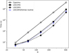 |
Fig. A.1. Comparison of Cppsimu (open circles) and LOC (filled black symbols) run times for CO line calculations, using a 3D model discretised onto a regular Cartesian grid. The x-axis gives the linear model size N, the models having N3 cells, and the y-axis shows the total run time, including the simulation of the radiation field and the solving of the equilibrium equations. The figure also shows LOC run times when the ray-tracing on the Cartesian grid is made with the more complex routines needed for octree grids. |
For N = 128 − 256, LOC run on a six-core CPU provides a speed-up of ∼6.0 compared to the Cppsimu. This suggests good parallelisation for the six-core CPU, although the number is affected by many implementation details in the two programs (and even the OpenCL version used). The speed-up could have been expected to be smaller because the average clock frequency is lower during the multi-core LOC run (because of the thermal limits of the processor and the laptop) and because Cppsimu simulates all transitions in one go and thus does not repeat the ray-tracing calculations for each transition separately. The speed-up provided by the GPU is ∼12.9 over the single-core Cppsimu run and thus more than a factor of two over the LOC run on the six-core CPU. The slightly smaller speed-up at N = 5123 may be affected by the increased disc usage.
Both Cppsimu and LOC are optimised to limit the radiation field updates to the velocity channels where the local absorption or emission line profile is significantly above zero. In the turbulent ISM model, the local line profile is typically much smaller than the full bandwidth of 50 km s−1. This means that the geometrical ray-tracing has a relatively high cost relative to the actual RT updates, in spite of the nominally large number of 512 velocity channels. As was seen in the case of 1D models (Appendix A.1), the relative performance of LOC improves if the number of floating point operations is higher than the data volume, for example if the local absorption or emission profiles covered a larger fraction of the bandwidth.
A.3. Three-dimensional octree grids
In the case of octree grids, the cost associated with the creation and storage of rays and the more complex path calculations can be significant. In LOC, each ray is processed by a single work group, and the updates to the different velocity channels are parallelised between the work items of that work group. The creation and tracking of ray paths are delegated to a single work item, which means that during those computations, the other work items of the work group remain idle. Therefore the efficiency of parallelisation would again increase if the number of velocity channels were larger (e.g. as in the case of spectra with hyperfine structure).
Figure A.1 shows the run times also for the case where the grid is Cartesian, but we use the more complex ray-tracing routines needed for octree grids. The overhead from the more complex path calculations is clear, even when the grid itself does not yet have any refinement.
We examined further how the run times depend on the number of hierarchy levels and the total number of cells in the octree grid. We used a root grid of 643 or 1283 cells and 0–3 additional levels, up to the full spatial resolution of the original 5123 model cloud. The other run parameters are the same as in Appendix A.2.
Figure A.2 shows the run times as a function of the number of cells in the model. Corresponding to each number of hierarchy levels NL, there are two cases in which either 10% or 30% of the cells of the previous hierarchy level were refined, thus resulting in a different total number of cells. When the percentage is 10%, there is a nearly equal number of cells on each refinement level (one tenth of the cells are split into eight cells each). When the percentage is 30%, most cells reside at higher hierarchy levels (i.e. are smaller in physical size). The run times are seen to remain almost directly proportional to the number of cells, and little additional cost is associated with deeper hierarchies.
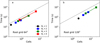 |
Fig. A.2. Comparison of LOC run times on a GPU for different octree grids. The octree hierarchies have NL = 1 − 4 levels and a root grid of 643 (frame a) or 1283 (frame b) cells. The solid lines connect two cases where either 10% or 30% of the cells of the previous level are refined. The dotted lines indicate the slope of one-to-one scaling between the run time and the number of cells. |
Appendix B: Converge tests with HCO+ and HCN
In Sect. 3.3.2, the 12CO RT calculations indicated that (when ALI is used) an increased spatial resolution may lead to some decrease in the rate at which the level populations converge. Figure B.1 shows results for the same cloud model in the case of the HCO+ molecule. The density dependence of the HCO+ fractional abundances is similar to that used for 12CO, but scaled to a maximum value of 5 × 10⁻⁹. Similar abundances have been observed in dense and translucent clouds, although the average value in the TMC 1 cloud is slightly higher (Fuente et al. 2019). However, in this test the main point is that the optical depths are sufficiently large so that a number of iterations is needed to reach the convergence. Figure B.1 shows the change in average errors as a function of the number of iterations, comparing the NL = 3 and NL = 4 discretisations. Although HCO+ remains sub-thermally populated, the highest Tex residuals are initially observed at intermediate densities. In later iterations (e.g. iteration 7), the largest errors are at the highest densities. Similar to the 12CO results (Fig. 4), the convergence is again slower in the case of the finer spatial discretisation (NL = 4).
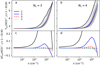 |
Fig. B.1. Average HCO+(1–0) excitation temperature as a function of density in the large-scale ISM simulation (cf. Fig. 4). The left and right frames show the results for different spatial discretisations (NL = 3, 4). The grey bands correspond to the 1%–99% and 10%–90% Tex intervals. The legend shows the colours that correspond to the different number of iterations. The lower frames show the Tex errors over iterations 1–7, estimated relative to the final values after 12 iterations. The horizontal dashed black line shows the ΔTex = 0 K level. |
Figure B.2 shows a final test with the HCN molecule. Here we used only the NL = 3 model, but we plot the convergence for both the J = 1 − 0 and J = 3 − 2 transitions. The hyperfine structure is taken into account only for the J = 1 − 0 transition, assuming LTE conditions between its components. The maximum abundance of HCN was set to 5 × 10⁻⁹, which in this case results in good convergence in fewer than ten iterations. The Tex residuals are initially higher for the higher transition, but the final accuracy is similar for both transitions.
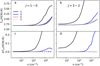 |
Fig. B.2. As Fig. B.1, but showing convergence for the HCN J = 1 − 0 (left frames) and J = 3 − 2 (right frames) transitions in the case of the NL = 3 model. |
Appendix C: Continuum RT calculations
In Sect. 3.3, the line calculations were compared with synthetic dust emission maps. The continuum calculations use the same octree-discretisation as the line calculations. The model is illuminated externally by a radiation field that corresponds to conditions in the solar neighbourhood (Mathis et al. 1983). The dust properties are those of the RV = 5.5 model of Weingartner & Draine (2001), as implemented in the DustEM package8.
The dust emission was calculated with the SOC program (Juvela 2019), assuming sub-millimetre emission from large grains at an equilibrium temperature. Compared to line transfer, the continuum RT calculations are faster even though Monte Carlo methods were used. By using photon-splitting techniques, the noise of the dust temperature estimates increases only linearly with the discretisation level, instead of the normal factor-of-two increase per discretisation level. This is true as long as the average optical depths are low and scatterings do not significantly reduce the photon flux into the densest regions. This is true for the present models and significantly saves run time. The noise in the computed dust temperatures was δTd ∼ 0.1 K at the highest refinement level. The computed maps represent the surface brightness of dust emission at the monochromatic wavelength of 250 μm.
All Figures
|
Fig. 1. Illustration of the creation of rays for a refined region. Rays a − e give a uniform sampling at the coarser level. Rays s and u are added for the refined region, using the information that ray c has of the radiation field at the upstream boundary of the refined cell. |
| In the text | |
|
Fig. 2. Comparison of 1D LOC results for cloud models presented in van Zadelhoff et al. (2002). The plots show the radial excitation temperature profiles of the HCO+J = 1 − 0 and J = 4 − 3 transitions for Model 2a and the optically thicker Model 2b. The LOC results are plotted with hashed red lines, the results of the Monte Carlo code Cppsimu are shown in blue and the other results (van Zadelhoff et al. 2002) in black (with different line types). In frame d, the cyan line shows LOC results for an alternative interpretation of the problem set-up. |
| In the text | |
|
Fig. 3. Comparison of NH3(1, 1) excitation temperatures and spectra for a spherically symmetric cloud. Frame a shows the radial Tex profiles computed with 1D versions of the Cppsimu and LOC programs and with the 3D version of LOC. The LOC runs use either a Cartesian grid with 643 cells or the same with two additional levels of refinement. Frame b compares the spectra observed towards the centre of the model. A zoom into the peak of the main component is shown in the inset. The lower plots show the ratio of Tex values (frame a) and the difference between the LOC and Cppsimu TA values (frame b), with the colours listed in frame a. |
| In the text | |
|
Fig. 4. Average 12CO(1–0) excitation temperatures in different density bins in the large-scale ISM simulation. The colours correspond to the situation after a given number of iterations, as indicated in the legend. The left frames show results for a model with a of 2563 cell root grid and NL = 3, and the right frame shows this for the same model with NL = 4. For a given density, the grey bands indicate the 1%-99% and 10%–90% intervals of the Tex values. The lower plots show the differences in the Tex values between iterations 1-5 and the seventh iteration (an approximation of the fully converged solution). The horizontal dashed black line corresponds to the ΔTex = 0 K level. |
| In the text | |
|
Fig. 5. Comparison of dust and line emission for a large-scale ISM simulation. The frames show the model column density (frame a), the computed 250 μm surface brightness of dust emission (frame b), and the13CO(1–0) line area (frame c). The white square in frame c indicates an area selected for closer inspection. |
| In the text | |
|
Fig. 6. Comparison of LTE (frame a) and non-LTE (frame b) predictions of W(13CO) for a region within the large-scale ISM simulation. The ratio of the LTE and non-LTE maps is shown in frame c. The corresponding histograms of W(13CO) values (above 10−3 K km s−1) are shown in frame d. The selected region is indicated in Fig. 5c with a white box. |
| In the text | |
|
Fig. 7. Dust and 13CO line emission as functions of column density of the large-scale ISM simulation. The blue 2D histogram shows the distribution of the 13CO line area vs. the true column density. The colour bar indicates the number of pixels in the original line emission maps per 2D histogram bin. The corresponding distribution of 250 μm surface brightness vs. column density (right-hand axis) is shown with red contours. The contour levels correspond to log10npix = 0.5, 1, 2, and 3 for the number image pixels npix per 2D histogram bin. The number of 2D bins is the same as for the 250 μm surface brightness histogram. |
| In the text | |
|
Fig. 8. Power spectra from synthetic observations of the large-scale ISM simulation. The power P is calculated for the true column density, the 250 μm dust surface brightness, and for three versions of 12CO line-area maps. The 12CO emission corresponds either to a constant abundance of χ0 = 10−4 and LTE conditions or to the Eq. (4) abundances with LTE or non-LTE calculations. The grey lines correspond to least-squares fits and extend over the range of the fitted spatial frequencies. |
| In the text | |
|
Fig. A.1. Comparison of Cppsimu (open circles) and LOC (filled black symbols) run times for CO line calculations, using a 3D model discretised onto a regular Cartesian grid. The x-axis gives the linear model size N, the models having N3 cells, and the y-axis shows the total run time, including the simulation of the radiation field and the solving of the equilibrium equations. The figure also shows LOC run times when the ray-tracing on the Cartesian grid is made with the more complex routines needed for octree grids. |
| In the text | |
|
Fig. A.2. Comparison of LOC run times on a GPU for different octree grids. The octree hierarchies have NL = 1 − 4 levels and a root grid of 643 (frame a) or 1283 (frame b) cells. The solid lines connect two cases where either 10% or 30% of the cells of the previous level are refined. The dotted lines indicate the slope of one-to-one scaling between the run time and the number of cells. |
| In the text | |
|
Fig. B.1. Average HCO+(1–0) excitation temperature as a function of density in the large-scale ISM simulation (cf. Fig. 4). The left and right frames show the results for different spatial discretisations (NL = 3, 4). The grey bands correspond to the 1%–99% and 10%–90% Tex intervals. The legend shows the colours that correspond to the different number of iterations. The lower frames show the Tex errors over iterations 1–7, estimated relative to the final values after 12 iterations. The horizontal dashed black line shows the ΔTex = 0 K level. |
| In the text | |
|
Fig. B.2. As Fig. B.1, but showing convergence for the HCN J = 1 − 0 (left frames) and J = 3 − 2 (right frames) transitions in the case of the NL = 3 model. |
| In the text | |
Current usage metrics show cumulative count of Article Views (full-text article views including HTML views, PDF and ePub downloads, according to the available data) and Abstracts Views on Vision4Press platform.
Data correspond to usage on the plateform after 2015. The current usage metrics is available 48-96 hours after online publication and is updated daily on week days.
Initial download of the metrics may take a while.