| Issue |
A&A
Volume 678, October 2023
|
|
|---|---|---|
| Article Number | A175 | |
| Number of page(s) | 12 | |
| Section | Numerical methods and codes | |
| DOI | https://doi.org/10.1051/0004-6361/202347376 | |
| Published online | 20 October 2023 | |
Self-consistent dust and non-LTE line radiative transfer with SKIRT
1
Sterrenkundig Observatorium, Universiteit Gent,
Krijgslaan 281 S9,
9000
Gent,
Belgium
e-mail: This email address is being protected from spambots. You need JavaScript enabled to view it.
2
Department of Physics, Graduate School of Science, The University of Tokyo,
7-3-1 Hongo,
Bunkyo-ku, Tokyo
113-0033,
Japan
3
Institute of Space and Astronautical Science, Japan Aerospace Exploration Agency,
3-1-1 Yoshinodai,
Chuo-ku, Sagamihara, Kanagawa
252-5210,
Japan
4
Institute of Astronomy, KU Leuven,
Celestijnenlaan 200D,
3001
Leuven,
Belgium
5
Graduate School of Science and Engineering, Kagoshima University,
1-21-35 Korimoto,
Kagoshima, Kagoshima
890-0065,
Japan
6
Research Center for Space and Cosmic Evolution, Ehime University,
2-5 Bunkyo-cho,
Matsuyama, Ehime
790-8577,
Japan
7
Faculty of Science, Hokkaido University, Kita-10 Nishi-8,
Kita-ku, Sapporo, Hokkaido
060-0810,
Japan
8
Theoretical Astrophysics, Department of Earth and Space Science, Osaka University,
1-1 Machikaneyama,
Toyonaka, Osaka
560-0043,
Japan
9
Kavli IPMU (WPI), The University of Tokyo,
5-1-5 Kashiwanoha,
Kashiwa, Chiba
277-8583,
Japan
10
Department of Physics and Astronomy, University of Nevada, Las Vegas,
4505 S. Maryland Pkwy,
Las Vegas, NV
89154-4002,
USA
Received:
5
July
2023
Accepted:
3
September
2023
Abstract
We introduce Monte-Carlo-based non-local thermodynamic equilibrium (non-LTE) line radiative transfer calculations in the three-dimensional (3D) dust radiative transfer code SKIRT, which was originally set up as a dust radiative transfer code. By doing so, we developed a generic and powerful 3D radiative transfer code that can self-consistently generate spectra with molecular and atomic lines against the underlying continuum. We tested the accuracy of the non-LTE line radiative transfer module in the extended SKIRT code using standard benchmarks. We find excellent agreement between the S KIRT results, the published benchmark results, and the results obtained using the ray-tracing non-LTE line radiative transfer code MAGRITTE, which validates our implementation. We applied the extended SKIRT code on a 3D hydrodynamic simulation of a dusty active galactic nucleus (AGN) torus model and generated multiwavelength images with CO rotational-line spectra against the underlying dust continuum. We find that the low-J CO emission traces the geometrically thick molecular torus, whereas the higher-J CO lines originate from the gas with high kinetic temperature located in the innermost regions of the torus. Comparing the calculations with and without dust radiative transfer, we find that higher-J CO lines are slightly attenuated by the surrounding cold dust when seen edge-on. This shows that atomic and molecular lines can experience attenuation, an effect that is particularly important for transitions at mid- and near-infrared wavelengths. Therefore, our self-consistent dust and non-LTE line radiative transfer calculations can help the observational data from Herschel, ALMA, and JWST be interpreted.
Key words: radiative transfer / ISM: molecules / methods: numerical / infrared: ISM
© The Authors 2023
 Open Access article, published by EDP Sciences, under the terms of the Creative Commons Attribution License (https://creativecommons.org/licenses/by/4.0), which permits unrestricted use, distribution, and reproduction in any medium, provided the original work is properly cited.
This article is published in open access under the Subscribe to Open model. This email address is being protected from spambots. You need JavaScript enabled to view it. to support open access publication.
1 Introduction
Continuum and spectroscopic observations can reveal a wealth of information on the dusty and gaseous medium for many astrophysical objects, such as the atmospheres of stars and exo-planets, protoplanetary disks and star-forming regions, and the interstellar medium (ISM) of galaxies. Continuum observations at infrared (IR) and submillimeter wavelengths can be used to determine the mass and temperature distribution of the dust in the ISM (Galliano et al. 2018). Doppler shifts of molecular and atomic lines provide powerful clues to understanding gas kinematics (Bland-Hawthorn & Gerhard 2016), and the line ratio provides us with thermal conditions and chemical composition in the gas (Wolfire et al. 2022).
Today, state-of-the-art facilities such as the James Webb Space Telescope (JWST) and the Atacama Large Millimeter/submillimeter Array (ALMA) provide us with high-quality spectroscopic and photometric data, which reveal various astro-physical phenomena on the dust, atoms, and molecules within the ISM of galaxies (e.g., Álvarez-Márquez et al. 2023; Rich et al. 2023; Liu et al. 2023; Meidt et al. 2023; Appleton et al. 2023; Schinnerer et al. 2023; Leroy et al. 2023). For the interpretation of these observational data, a basic approach is a comparison between observations and three-dimensional (3D) hydrodynamic simulations, which predict the spatial distribution, velocity structure, and physical conditions of the multiphase ISM in galaxies (e.g., Gatto et al. 2017; Kim & Ostriker 2018; Kado-Fong et al. 2020; Rathjen et al. 2021; Kim et al. 2023), although inferring the physical properties of the ISM even from these high-quality observations is not trivial. Observations are always projections along the line of sight, and detailed information about the complex 3D structure of the objects under study is lost. Moreover, differential dust attenuation along the line of sight affects the relative strengths of the lines and complicates the interpretation. In addition, the observational analysis methods used to extract physical information from the observed properties invariably involve assumptions and systematic uncertainties – for example, calibrations of the continuum subtraction or assumption of local thermodynamic equilibrium (LTE) for the excitation states in molecules and atoms. Therefore, forward modeling synthetic observational data from hydrodynamic simulations is an important means to help us understand the observational data and assess the importance of assumptions and systematics.
For an accurate estimation of the line intensities from atoms and molecules, we need non-LTE line radiative transfer codes that self-consistently calculate, at every location in the simulation volume, the radiation field and the level populations considering collisional and radiative transitions due to external radiation. Such non-LTE calculations are essential because the ISM is not only composed of dense gas clouds in LTE conditions but also diffuse gas clouds exposed to radiation. Over the past years, many non-LTE line radiative transfer codes, most of them ray-tracing codes, have been developed, including RATRAN (Hogerheijde & van der Tak 2000), LIME (Brinch & Hogerheijde 2010), TORUS (Rundle et al. 2010), MOLLIE (Keto & Rybicki 2010), 3D-PDR (Bisbas et al. 2012), LOC (Juvela 2020), and MAGRITTE (De Ceuster et al. 2020). To calculate radiation fields, these codes backtrack the paths of incident rays on each point and average the numerically calculated intensities of the incoming rays. While these codes accurately calculate radiation fields when the cosmic microwave background (CMB) is dominant as external radiation, it is difficult to handle dust radiative processes including scattering processes. As a result, their calculations have never involved dust radiative transfer, and they are not good at estimating spectra of atomic and molecular lines in the near- and mid-infrared (NIR and MIR, respectively) wavelength ranges, where dust emission is dominant.
On the other hand, to generate mock continuum IR dust observations, dust radiative transfer codes are required. Typically, they are stochastic Monte Carlo codes; they simulate the emission of heating sources and the absorption, scattering, and thermal emission by the dust using a finite number of photon packets; and they calculate radiation fields by averaging the intensities of the photon packets passing through each cell. In this way, the temperature distribution of the dust grains and corresponding emission are estimated at every location in the simulation volume. Three-dimensional dust radiative transfer has experienced a strong development over the past two decades (Steinacker et al. 2013), and nearly all modern 3D dust radiative transfer codes, such as DIRTY (Gordon et al. 2001), SKIRT (Baes et al. 2011), HYPERION (Robitaille 2011), RADMC-3D (Dullemond et al. 2012), POLARIS (Reissl et al. 2016), and SOC (Juvela 2019), employ the stochastic Monte Carlo method.
Ideally, dust and non-LTE line radiative transfer postprocessing should be done with a single code. This has the obvious advantage that the calculations can be done simultaneously and self-consistently. An accurate estimation of the dust emission is essential for atomic and molecular lines against the dust continuum since the dust emission can excite them (Matsumoto et al. 2022). In fact, some observations report that IR radiation pumps the rotational and vibrational states of molecules (e.g., Aalto et al. 2007; Imanishi et al. 2016, 2017; Runco et al. 2020). Moreover, dust radiative transfer is also needed to calculate the attenuation of the line emission itself, in particular for NIR and MIR lines such as the OH and H2 rotational lines and CO rovibrational lines. To simultaneously perform non-LTE line and dust continuum radiative transfer, the Monte Carlo approach seems to be the most suitable option. The technique is conceptually straightforward and intrinsically 3D, which makes it naturally suitable for complex 3D structures. Moreover, scattering is, contrary to ray-tracing methods, easily incorporated in the Monte Carlo framework (Steinacker et al. 2013).
There are some challenges to the establishment of a joint line and continuum Monte Carlo code, however. The main issue for Monte Carlo radiative transfer is that the radiation fields always contain Monte Carlo noise, which leads to slow convergence. In particular, due to the random nature of the propagation direction of the photon packages, some cells are visited less frequently than others, which results in a slower convergence rate. A second challenge is that negative opacities can be encountered in non-LTE line radiative transfer. Indeed, inverted level populations can lead to net negative opacity coefficients and stimulated emission, and standard Monte Carlo radiative transfer methods cannot handle this.
SKIRT1 (Baes et al. 2011; Camps & Baes 2015, 2020) is a state-of-the-art 3D Monte Carlo code. Originally set up as a dust radiative transfer code, it has now evolved to a more generic radiative transfer code that also includes capabilities beyond dust radiative transfer (e.g., Camps et al. 2021; Gebek et al. 2023; Vander Meulen et al. 2023) and is widely applied to generate synthetic ultraviolet (UV)-millimeter broadband fluxes, images, spectral energy distributions (SEDs), and polarization maps for simulated galaxies and tori of active galactic nuclei (AGNs; e.g., Stalevski et al. 2012, 2023; Camps et al. 2016, 2022; Trayford et al. 2017; Granato et al. 2021; Kapoor et al. 2021; Vandenbroucke et al. 2021; Lahén et al. 2022; Trcka et al. 2022; Hsu et al. 2023). However, non-LTE line radiative transfer calculations have not been implemented in SKIRT so far.
Thanks to several characteristics of the code already implemented, the extension of SKIRT to a joint non-LTE line and dust continuum radiative transfer code is possible. To deal with Monte Carlo noise and poor convergence of the radiation field, SKIRT is equipped with a hybrid parallelization strategy that allows for the efficient launching of a huge number of photon packets (Verstocken et al. 2017; Camps & Baes 2020). Various Monte Carlo acceleration and variance-reduction techniques have been implemented to increase the number of photon packets crossing each cell and to stimulate the absorption rates in less frequently visited cells (e.g., Baes et al. 2011, 2016; Steinacker et al. 2013; Camps & Baes 2020). To enable negative opacities in the Monte Carlo loop, the technique of explicit absorption has been introduced (Baes et al. 2022). This technique treats absorption along any photon packet path deterministically, while only scattering is treated stochastically. It boosts the efficiency of the Monte Carlo radiative transfer loop and is fully compatible with the negative opacities corresponding to stimulated emission.
In this paper, we present the implementation of non-LTE line radiative transfer in SKIRT and thus its extension to a self-consistent dust and non-LTE line radiative transfer code. This paper is organized as follows. Section 2 describes the procedure of the self-consistent non-LTE line and dust radiative transfer calculation. In Sect. 3, we investigate whether the Monte-Carlo-based non-LTE line radiative transfer implemented in SKIRT can achieve an accuracy comparable to other codes using the standard benchmarks of van Zadelhoff et al. (2002). Section 4 demonstrates mock observations for CO lines against the dust continuum based on a 3D hydrodynamic simulation of a multiphase AGN torus and investigates the effect of dust attenuation on CO lines. Section 5 discusses the characteristics, strengths, and limitations of our self-consistent dust and non-LTE line radiative transfer code and presents our conclusions.
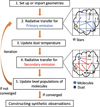 |
Fig. 1 Execution flow of self-consistent dust and non-LTE line radiative transfer calculation in SKIRT and the schematic pictures of the radiative transfer of primary and secondary emission. Blue and red arrows represent primary and secondary emission, respectively. |
2 Dust and non-LTE line radiative transfer in SKIRT
SKIRT is currently primarily a dust radiative transfer code, but is ideally suited to be extended for self-consistent dust and non-LTE RT. Indeed, some important features have already been introduced, such as Doppler shifts of both the emitting sources and the medium, and iterative schemes for the calculation of the radiation field and the dust temperature distribution (Camps & Baes 2020). The modified Monte Carlo radiative transfer scheme of explicit absorption has also been implemented in the latest version of SKIRT (Baes et al. 2022). This scheme allows us to handle negative opacities by separately operating the absorption and stimulated emission numerically and the scattering process stochastically. Thanks to these features already implemented, the extension to self-consistent dust and non-LTE line radiative transfer only requires the implementation of the emissivity, the opacity, and the line profile of atoms and molecules, and the framework to calculate the level populations (see Appendix A for a formal summary).
We have set up an algorithm for iteratively performing the two-step radiative transfer calculations, updating dust temperatures, and solving statistical equilibrium equations. Figure 1 illustrates the execution flow of the dust and non-LTE radiative transfer in SKIRT. The first step consists of setting up the input parameters for the model. In most cases, this comes down to importing physical values from a hydrodynamic simulation snapshot. The physical properties that the radiative transfer routine requires are the number density of molecules or atoms nmol, the number densities of collision partners np, the kinetic gas temperature Tkin, the microturbulence υturb, and the densities and optical properties of the different dust species. It is also possible to use any analytical or semi-analytical geometries built into SKIRT, including shells, exponential disks, smooth and clumpy tori, etc. (Baes & Camps 2015). We also need to choose an appropriate grid to discretize the medium (Camps et al. 2013; Saftly et al. 2013, 2014) and to set the different wavelength grids to be used in the different phases of the simulation (see Camps & Baes 2020, for details). For the line RT, we need to include a finely discretized grid around the wavelength of each transition line.
In the second step, we launch photon packets in the so-called primary emission cycle. SKIRT works with two types of photon packets: primary and secondary emission photon packets. Primary emission photon packets are launched from primary sources, which are sources for which the emission spectrum and luminosity are fixed at the start of the simulation. This includes stars or stellar populations, AGNs, the CMB, or a user-defined background source. Secondary emission photon packets are those launched from sources for which the emission profile depends on the local radiation field, such as the dust and gas medium. For estimating the radiation fields corresponding to primary emission, a large number of primary emission photon packets are launched, with a wavelength, initial position, and propagation direction determined by the source characteristics. The photon packets interact with the dust grains and the atoms and molecules in the medium. The optical properties of the dust grains are independent of the radiation field, but those of the atoms and molecules are not, as these depend on the radiation-field-dependent level populations. The initial level populations of atoms and molecules are assumed in LTE, and the initial opacity and emissivity are calculated.
When the primary emission cycle has terminated, we can, in every cell of our grid, calculate the radiation field from primary emission. we accomplish this calculation by averaging the intensity of all photon packets passing through each cell, as opposed to just considering information at the cell centers. Subsequently, we determine the temperature distribution of the different dust grains. The user can choose whether to use local thermal equilibrium or stochastic heating for the dust temperature distribution and the corresponding dust emission spectra (Camps et al. 2015).
The fourth step consists of the radiative transfer corresponding to secondary sources, which in the present case comes down to photon packages from the dust and gas. Similar to the second step, a large number of photon packets are launched, and each of them is followed through the medium. Contrary to the primary emission cycle, the assigned energy carried by each secondary photon packet is variable in every iteration of the simulation, since it depends on the emission spectrum of the medium, which in turn depends on the level populations of atoms and molecules and the dust temperature distribution. For a given medium cell, the total secondary luminosity is the sum of the total dust luminosity and the joint luminosity corresponding to the spontaneous emission of all line transitions. For a given transition line, the total luminosity is given by
 (1)
(1)
where λline, Aul, nu, and Vcell are the rest wavelength of the transition line, the Einstein coefficients for spontaneous emission from the upper level u to lower level l, the number density of the upper level of the atoms or molecules, and the volume of the cell, respectively. h and c are the Planck constant and the speed of light, respectively. The wavelength of each photon packet λ is determined according to the Gaussian distribution in the rest frame of the cell and adjusted for any Doppler shifts caused by the bulk motion at the cell. The probability function of the Gaussian distribution, which is the same as the line profile ϕline, is expressed as
 (2)
(2)
The wavelength dispersion σline is given by
 (3)
(3)
where k and ms are the Boltzmann constant and the atomic or molecular mass, respectively. The first term and the second term under the square root represent the sound speed of the thermal motion of the gas and the assumed non-thermal motion of clouds in each grid, respectively. After launching all secondary source photon packets and following their life cycle through the medium, we can calculate the radiation field corresponding to the secondary emission.
The fifth step corresponds to the most important extension of the SKIRT code. Once the radiation fields from primary  and secondary emission
  in each cell are estimated, we calculate the combined radiation field,
 (4)
(4)
and we determine the mean intensity at each line transition
 (5)
(5)
To obtain the level populations, we assume that the timescale to the equilibrium of transitions in the level populations is shorter than the dynamical timescale of the system. We can formulate the statistical equilibrium equations as follows,
![Mathematical equation: $ \matrix{ {\sum\limits_{j lt; i}^{{N_{{\rm{lp}}}}} {{n_i}{A_{ij}} - \sum\limits_{j > i}^{{N_{{\rm{lp}}}}} {{n_j}{A_{ji}} + \sum\limits_{j \ne i}^{{N_{{\rm{lp}}}}} {\left[ {\left( {{n_i}{B_{ij}} - {n_j}{B_{ji}}} \right){{\bar J}_{{\rm{line}}}}} \right]} } } } \hfill \cr { + \sum\limits_{j \ne i}^{{N_{{\rm{lp}}}}} {\sum\limits_p^{{N_{\rm{p}}}} {\left[ {{n_i}{C_{ij}}\left( {{n_{\rm{p}}},{T_{{\rm{kin}}}}} \right) - {n_j}{C_{ji}}\left( {{n_{\rm{p}}},{T_{{\rm{kin}}}}} \right)} \right] = 0} } ,} \hfill \cr } $](/articles/aa/full_html/2023/10/aa47376-23/aa47376-23-eq8.png) (6)
(6)
where Nlp and Np are the numbers of energy states and collision partners, respectively. Bul, Blu, and Cij are the Einstein coefficients for stimulated emission and absorption, and the collisional coefficients, respectively (see also Appendix B). The upper and lower terms on the left side represent radiative and collisional transition rates, respectively. Equation (6) forms a matrix equation with the level populations ni as the unknowns. To solve this matrix equation, we use the LU decomposition method. Once the level populations are updated, the absorption coefficients and the luminosity of the atoms and molecules are also updated (see Appendix A and Eq. (1), respectively).
After finishing the fifth step, we return to the second one, the primary emission radiative transfer calculations. Indeed, with the level populations of atoms and molecules updated, the absorption coefficients also changed. This naturally leads to an iterative cycle of calculations from step 2 to step 5 until the solution is converged. To accelerate the iterative calculations, Ng acceleration (Ng 1974) is implemented in SKIRT but not used in the default configuration.
We have implemented two convergence criteria in SKIRT, and depending on their specific use case, users can select which one they use (or they can implement a different one). The first one employs the local convergence parameter ϵm, given by
 (7)
(7)
where  represents the number density at the energy states i in cell number m at iteration stage k. Our default convergence criterion is that ϵm must be below 0.05 for 99.9% of all cells in the simulation volume, but the fraction of converged cells and the threshold value can be defined by users.
An alternative convergence criterion implemented employs the total convergence parameter ϵtotal, given by
 (8)
(8)
where  represents the total number density in the entire simulation volume at the energy state i at iteration stage k. Our default setting is that iterations have converged when ϵtotal is below 10−4, but, again, it can be chosen by the user. We note that the total convergence parameter minimizes the contribution of Monte Carlo noise and is, therefore, suitable as a convergence criterion in Monte Carlo radiative transfer simulations.
Finally, when convergence has been reached, we proceed to the final step in our Monte Carlo radiative transfer algorithm, that is, the construction of synthetic observations. We again perform radiative transfer calculations for primary and secondary emission in steps 2 and 4 based on the converged absorption coefficients and emissivity of dust, atoms, and molecules. Photon packets escaping from the system are detected by synthetic instruments located at arbitrary viewing points with user-defined characteristics such as field-of-view and spatial and wavelength resolution. For the specific case of joint dust and non-LTE line RT, we typically use instruments with a wide wavelength range consisting of relatively broad wavelength bins, but with narrow wavelength bins around the line centers. In order to boost the signal-to-noise in these narrow bins around the line centers, composite biasing in wavelength space can be employed (Baes et al. 2016; Camps & Baes 2020).
At this moment we have implemented non-LTE radiative transfer for two atoms and four molecules (C, C+, CO, OH, H2, and HCO+) in SKIRT. Relevant atomic and molecular properties are taken from the Leiden Atomic and Molecular Database2 (Schöier et al. 2005).
3 Benchmarks
To validate the non-LTE line radiative transfer in SKIRT, we run the code on four well-defined test problems presented by van Zadelhoff et al. (2002). We compare our results with their reference results and those obtained by a modern, pure ray-tracing non-LTE line radiative transfer code, MAGRITTE (De Ceuster et al. 2020). In the MAGRITTE simulations, the convergence criterion is that ϵm < 10−10 for 99.5% of all cells in the simulation volume through all problems. The parameter files of these benchmarks for SKIRT3 are publicly available.
3.1 Problem 1a/1b
The first set of two models is originally taken from Dullemond & Turolla (2000) and corresponds to a simple spherically symmetric shell without radial velocities. The shell is populated by molecular hydrogen and by an artificial two-level molecule specified by
 (9)
(9)
 (10)
(10)
 (11)
(11)
 (12)
(12)
 (13)
(13)
where g0, g1, and K10 are the degeneracy of the lower and upper energy levels and the collisional de-excitation coefficient, respectively. ∆E and Mmol are the energy gap between the two energy levels of the molecule and mass expressed in units of the hydrogen atom mass, respectively. The molecular mass is determined so that the thermal velocity is 150 m s−1 at the kinetic temperature of 20 K.
The artificial molecules and the molecular hydrogen, which acts as the collisional partner, are distributed in a spherical shell with inner radius r0 = 1.0 × 1015 cm and outer radius r1 = 7.8 × 1018 cm. The radial profile of the molecular hydrogen number density is given by a power law of
 (14)
(14)
where r is the radius, and (r0) = 2.0 × 107 cm−3. The kinetic temperature and micro-turbulence of the molecules are constant at 20 K and zero, respectively. The abundances of the artificial molecules in problems 1a and 1b are Xa = 10−8 and Xb = 10−6, respectively, and the total optical depths at the line center are 60 and 4800, respectively. The shell is illuminated by the external radiation from the CMB.
For the SKIRT calculations, we have set up a spherical grid with 50 and 500 logarithmically spaced shells for problems 1a and 1b, respectively (the dependency of the results of problem 1b on the number of shells is investigated in Sect. 3.3.1). We adopted 108 photon packets for these problems, and the convergence criterion is that ϵm < 0.001 for 99% of all cells in the simulation volume. To reach convergence in the level populations, SKIRT requires 42 and 694 iterations in problems 1a and 1b, respectively. On the other hand, MAGRITTE needs 34 and 379 iterations in problems 1a and 1b, respectively.
Figure 2 shows the comparison of the level populations among the different codes used in the van Zadelhoff et al. (2002) reference study (solid lines), SKIRT (dots) and MAGRITTE (dashed lines) for problems 1a and 1b. In these problems, the level populations at small radii are collisionally determined, while at large radii they are radiatively determined by the CMB. Since the shell in problem 1b is more optically thick than the one in problem 1a, the CMB radiation cannot penetrate deeply into the gas shell and as a result, the level populations of problem 1b are collisionally determined out to the larger radii. The level populations obtained with SKIRT agree with the reference results within the relative difference of 2 and 5% in problems 1a and 1b, respectively, while those obtained with MAGRITTE agree within the relative difference of 2% in both problems.
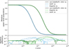 |
Fig. 2 Comparison of the relative population at the upper level obtained with SKIRT (dots) and MAGRITTE (dashed lines) and the reference results of van Zadelhoff et al. (2002; gray solid lines) for benchmark problem 1a (blue lines) and 1b (green lines). The level population is normalized by the total number density. The differences of MAGRITTE and SKIRT results relative to the reference results are shown in the bottom panel. |
3.2 Problem 2a/2b: A collapsing cloud in HCO+
The second set of two models is based on an inside-out collapse model presented by Shu (1977). These problems again assume a 1D spherical shell geometry, now with inner radius r0 = 1.0 × 1016 cm and outer radius r1 = 4.6 × 1017 cm, and with density, velocity, and temperature gradients and a non-constant microturbulence. The radial profiles of those physical values are shown in Fig. 2 of van Zadelhoff et al. (2002). The shell contains HCO+ molecules and H2 molecules which act as collisional partners. The HCO+ abundances in problems 2a and 2b are Xa = 10−8 and Xb = 10−6, respectively.
For the SKIRT calculations of these two benchmark problems, we have set up a 3D cubic box with 1003 cuboidal cells. The distribution of cells along each axis is chosen according to a power-law distribution to ensure smaller cells near the inner regions of the shell. For problems 2a and 2b, we use 2.2 × 10⁸ and 109 photon packets, respectively. We set the convergence criterion as that ϵm < 0.02 for 99.95% of all cells. To reach the convergence criterion, SKIRT requires 22 and 94 iterations in problems 1a and 1b, respectively. On the other hand, MAGRITTE needs 33 and 110 iterations in problems 1a and 1b, respectively.
Figure 3 shows the comparison of the J = 1 and J = 4 level populations of HCO+ among the different codes used in the van Zadelhoff et al. (2002) reference study (gray dashed lines), SKIRT (blue solid lines with dots) and MAGRITTE (yellow solid lines) for problems 2a and 2b. In both problems, the SKIRT results agree with those obtained with MAGRITTE within 20%. Given that the level populations obtained using different codes in van Zadelhoff et al. (2002) show relative differences of up to 20%, we argue that these tests validate SKIRT as a non-LTE line radiative transfer code.
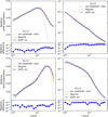 |
Fig. 3 Comparison of the relative HCO+ level population for benchmark problem 2a (upper panels) and 2b (bottom panels) at J = 1 (left) and J = 4 (right) obtained with SKIRT (blue solid lines with dots) and MAGRITTE (yellow solid lines) and the reference results of van Zadelhoff et al. (2002; gray dashed lines). The level population is normalized by the total number density. The relative differences between the MAGRITTE and SKIRT results are shown in the lower subpanels. |
3.3 Convergence of the radiation field in skirt: tests based on problem 1b
The iterative calculation in non-LTE line radiative transfer calculations plays an essential role in sharing radiation throughout the entire simulation box. However, if the optical thickness per cell becomes too large, photon packets are primarily absorbed within a single cell, which results in radiation fields that are no longer shared between neighboring cells. The solution consists of increasing the number of cells and/or the number of photon packets in the simulation, but this immediately affects the run-time and memory requirements.
In this subsection, we investigate two critical parameters, the number of grid cells and the number of photon packets that determine the stability of the radiation field. We use problem 1b of van Zadelhoff et al. (2002) for these tests; this problem is ideally suited for this test because of the combination of simplicity (we can use a 1D spherical grid in which all cells are concentric shells) and high optical thickness (τ ~ 4800 at the line center).
3.3.1 The number of cells
The limitation of the optical thickness in Monte Carlo dust radiative transfer calculations with SKIRT is τ < 75 (Camps & Baes 2018) while τ < 100 is required for the ray-tracing method (Hogerheijde & van der Tak 2000). However, it is not clear whether Monte-Carlo-based non-LTE line radiative transfer calculations also require τ < 75 for sharing the radiation fields. Here, we investigate the limitations of the optical thickness per cell by performing SKIRT on problem 1b with various numbers of grid cells.
The left panel of Fig. 4 compares the relative populations at the upper level of the artificial two-level molecule corresponding to calculations with different numbers of grid cells (Ncell = 50, 100, 200, and 400), and we consider the simulation with the highest number of cells as our ground truth result. We use 750 iterations, and the same number of photon packets in each iteration, 107. The populations corresponding to the calculations with smaller numbers of cells show larger deviations from the ground truth results, which implies that if the simulation box is not sufficiently divided, the radiation fields are no longer shared. For the calculation with Ncell = 400, the largest optical depth in any cell is 73.7, which suggests that non-LTE radiative transfer calculations in SKIRT require a similar optical-depth-per-cell constraint as dust radiative transfer calculations to reproduce accurate level populations.
On the other hand, the right panel of Fig. 4 shows the observed line profiles of the two-level molecule of problem 1b at the 1.6666mm transition, for different SKIRT simulations with Ncell = 50, 100, 200, and 400. The line profiles are not significantly different since only photon packets from the surface layer of the sphere can reach the observer because of the large optical thickness.
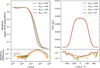 |
Fig. 4 Convergence tests for benchmark problem 1b for calculations with different cell numbers, as indicated in the top right corner of the left panel. Left: relative populations at the upper level. Right: observed line profiles corresponding to a distance of 1 Mpc from the sphere’s center. In both cases, the relative differences between each simulation and the reference simulation with 400 cells are shown in the lower panels. |
3.3.2 The number of photon packets
To investigate the required number of photon packets to solve problem 1b, we run a suite of SKIRT simulations with various numbers of photon packets. We use 500 cells and 750 iterations in each simulation.
The left panel of Fig. 5 compares the relative population at the upper level of the two-level molecule from problem 1b for SKIRT simulations with various numbers of photon packets (Np = 1 × 10⁴, 4 × 10⁵, and 1 × 10⁷). The solution corresponding to Np = 1 × 10⁷ is considered to be our ground truth. While the level population of the calculations with Np = 4 × 10⁵ is consistent with those with Np = 1 × 10⁷, that with Np = 1 × 10⁴ is not. The reason for this mismatch is that, for a small number of photon packets per cell (here Np/500), we cannot accurately express the shape of the line profile and the spectrum of the radiation field in each cell.
The right panel of Fig. 5 shows the comparison of the observed line profiles of problem 1b for the same set of three SKIRT simulations. Noise is noticeable in the line profiles corresponding to the calculation with Np = 4 × 10⁵. To calculate accurate radiation fields and produce correct level populations, we suggest at least the total number of photon packets of Np = 800 × Ncell × Nline, where Nline is the number of the transition lines of molecules or atoms in the calculations.
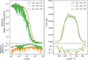 |
Fig. 5 Convergence tests for benchmark problem 1b for calculations with different photon packet numbers, as indicated in the top right corner of the left panel. Left: relative populations at the upper level. Right: observed line profiles corresponding to a distance of 1 Mpc from the sphere’s center. In both cases, the relative differences between each simulation and the reference simulation with 107 photon packets are shown in the bottom panels. |
4 Application to an AGN torus model
As a demonstration of the power of the new capabilities of SKIRT, we perform self-consistent dust and non-LTE line radiative transfer calculations based on an AGN torus simulation.
4.1 AGN torus model and SKIRT setup
Wada et al. (2016) modeled the structure of the AGN torus of the Circinus galaxy using a 3D Eulerian hydrodynamic simulation composed of a uniform Cartesian grid with 2563 cells. The simulation box is 32 pc on each side, corresponding to a cell resolution of 0.125 pc. The model incorporates the physics coupling radiative processes and hydrodynamics: UV and X-ray radiation from the accretion disk drives outflows in the polar direction of the AGN and generates a geometrically thick torus with complex dynamical structures around the AGN. Furthermore, the radiation heats the ambient gas and affects the chemical structure, which results in the formation of multiphase gas in the torus composed of molecular, atomic, and ionized phases. The abundances of 25 gas species including H, H2, H+, C, C+, and CO are calculated using the chemical network of Meijerink & Spaans (2005). The dust-to-gas mass ratio is assumed to be 0.01. We assume that supernova explosions occur at random locations in the equatorial plane with a rate of 0.014 yr−1, which helps to enhance the thickness of the torus (Wada et al. 2009).
The dust and CO emission of this AGN torus model has already been independently investigated by Wada et al. (2016, 2018), Uzuo et al. (2021), and Matsumoto et al. (2022). In these studies, the original data for the hydrodynamic simulation was reduced to half of the resolution due to the memory capacities of the radiative transfer codes used, and their simulations included uncertainties due to the reduced resolution. However, SKIRT can keep the original spatial resolution due to the efficient memory distribution implemented in the code (Camps & Baes 2020). In addition, SKIRT can reconstruct the original data using hierarchical octree grids, recursively subdividing the simulation box into 24 to 28 cells in each axis. Consequently, the number of cells does not increase so much, though the original spatial resolution is retained.
In our SKIRT run, we considered two sources of external radiation: the CMB and a central point source representing the AGN accretion disk. For this latter source, we assumed a power-law spectrum in the UV-to-optical wavelength range, which heats ambient dust. We note that free-free and synchrotron radiation expected to be emitted near the accretion disk is not taken into account in our model, as the radiation is not regarded as the dominant source of the submillimeter continuum emission of AGN (e.g., Tristram et al. 2022). We employ the Draine & Li (2007) dust model with silicate, graphite, and polycyclic aromatic hydrocarbon (PAH) grains, and considered stochastic heating. The microturbulence in each cell was assumed to be constant at 5 km s−1.
To illustrate the computational cost of the SKIRT simulations, we run two different simulations: (i) a pure dust radiative transfer simulation with the accretion disk as the external source and (ii) a self-consistent dust and CO line radiative transfer simulation with both the accretion disk and the CMB as external sources. We run the first simulation with 6 × 10⁸ and 1.5 × 10⁹ photon packets for the emission from the accretion disk and dust emission, respectively, and the second one with the additional 2.4 × 10⁹ and 1.5 × 10⁹ photon packets for CMB and the CO line emission, respectively. As a result, the second simulation adds 285% to the run times of each iteration in the first one. Moreover, the second simulation takes 10 times more iterations to reach convergence. Thus, the total run time of the second simulation increases as the iteration number and the number of total photon packets increase. In Sect. 4.2 we investigate the spectral features of the dust continuum and CO lines up to J = 20. In Sect. 4.3 we investigate the dust extinction effects on the CO lines by comparing the results of the calculations with and without dust.
4.2 CO rotational emission lines and dust continuum
Figure 6 shows the SKIRT simulation results. The panels on the first two rows show dust continuum maps corresponding to three different bands: the far-infrared (FIR) ALMA/Band 8, the MIR JWST/MIRI F1280W band, and the NIR JWST/NIRCam F200W band. The first and second rows correspond to face-on and edge-on views, respectively.
While the FIR radiation is emitted only from the cold dust extending on the dense disk in the torus (panels a and d), the MIR emission mainly comes from the inner region of the disk and the polar region of the torus (panels b and e). Finally, the NIR emission can only be clearly detected in the innermost region of the AGN torus in the face-on orientation (panel c). The emission is very faint in the edge-on view, as the emission is almost completely shielded by cold dust in the torus (panel f). These results are qualitatively consistent with Schartmann et al. (2014), in which the dust radiative transfer was performed with RADMC-3D (Dullemond et al. 2012) based on the hydrodynamic model presented by Wada (2012).
The panels on the third and fourth rows of Fig. 6 show integrated intensity maps of CO(1–0), CO(6–5), and CO(12–11) for face-on and edge-on views, respectively. Both the CO(1–0) and CO(6–5) emission extend to 10 pc on the vertical axis, tracing the geometrically thick molecular torus. Since the CO(6–5) emission originates from the molecular gas with kinetic temperatures of several tens K, it seems to trace a more puffed-up structure of the molecular torus compared to the CO(1–0) emission. On the other hand, the CO(12–11) emission comes from gas with kinetic temperatures higher than 100 K in the innermost region where the gas is heated by radiation from the accretion disk and the places where supernovae explode.
Figure 7 shows the total SED of the torus at various inclination angles (θ = 0°, 45°, and 90°). The contribution of dust continuum emission, PAH band emission, the 9.7 silicate feature, and CO rotational lines are clearly visible. The dust emission in the NIR to MIR wavelength range is more and more attenuated as the inclination angle increases since this emission originates from the hot dust in the innermost region of the AGN torus and is shielded by cold dust in the outer region (see also Fig. 6). The silicate feature is seen in emission at face-on and intermediate inclination, and in absorption in the edge-on view. At smaller inclination angles, higher-J CO emission lines are stronger since we directly observe highly excited CO emission from the gas in the inner region of the AGN torus, and the high CO lines are attenuated by dust.
Figure 8 shows the integrated line profiles of CO(1–0), CO(6–5), CO(12–11), and CO(15–14) observed at various inclination angles (θ = 0°, 45°, and 90°). As the inclination angle increases, the line profiles are broadened due to the Keplerian rotation of the AGN torus. In particular, the CO(1–0) emission line is observed as two separate profiles in the edge-on view, tracing the Keplerian motion of the cold gas. On the contrary, higher-J lines are observed as asymmetrical profiles including broad components at the inclination angles of θ = 45° and 90°, tracing the turbulent gas driven by radiation from the accretion disk and supernovae.
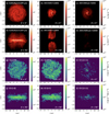 |
Fig. 6 Dust continuum images (first and second rows) and CO line emission maps (third and fourth rows) for the AGN torus model discussed in Sect. 4.1. Each image consists of 256 × 256 pixels with a pixel size of 0.125 pc. The images on the first and third rows are viewed face-on, and those on the second and fourth rows are viewed edge-on. |
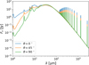 |
Fig. 7 Spectral energy distributions including CO rotational lines from J = 0 to J = 19 for the AGN torus simulation. The different lines correspond to SEDs seen at different inclination angles, as indicated in the legend. The observers are located at a fiducial distance of 4.2 Mpc, and a beam size of (32 pc)2 is used. |
4.3 Dust effects on CO lines
To demonstrate the importance of self-consistent dust and non-LTE line radiative transfer calculations, we perform SKIRT CO non-LTE radiative transfer calculations with and without dust. The presence of dust has two complementary effects on the line emission. On the one hand, it acts as a source term that affects the level populations; without dust, the CMB is the only external source term. Secondly, as shown in Fig. 7, it can affect the observed CO line strengths due to attenuation. To quantify the effect of dust, we compare the CO spectral line energy distribution (SLED), that is, an intensity function of the CO rotational emission lines with the different rotational levels normalized by the intensity of CO(1–0). CO SLEDs are commonly used as a diagnostic for the excitation of CO molecules (e.g., Panuzzo et al. 2010; van der Werf et al. 2010; Rangwala et al. 2011; Mashian et al. 2015).
Figure 9 compares the total CO SLEDs between the SKIRT models without dust and with dust. We chose the edge-on orientation to maximize the potential effect of dust attenuation. We find that the values of the SLED of the model with dust are slightly lower than those of the model without dust at the higher / values. The reason for this suppression of the high-J line intensities in the presence of dust is that the higher-J lines originate from the innermost region of the torus (see Fig. 6i), which are surrounded by the optically thick cold dust (Fig. 6d). We note that the excitation of CO molecules by the dust emission is not efficient in our simulations, although Matsumoto et al. (2022) imply that the vibrational and rotational excitation of CO molecules at higher energy states is caused by the dust continuum. This difference is due to the dust temperature near the equatorial plane. Matsumoto et al. (2022) estimated a higher dust temperature of several tens K using a simpler dust model and a different dust radiative transfer code, RADMC-3D, while the present radiative transfer calculations set the dust temperature at around 10 K. Observations with ALMA and JWST will be useful to determine whether the excitation of CO molecules by dust emission is really effective.
We conclude that self-consistent dust and non-LTE line radiative transfer calculations with SKIRT show that higher-J CO lines can be attenuated by dust, changing the shape of the SLED. For the rotational CO lines considered here, this attenuation is still modest as even the higher-J rotational lines are situated in regions with modest dust optical depths. However, the same effect can be much more pronounced for atomic and molecular lines at shorter wavelengths, such as H2, OH rotational, and CO rovibrational lines. We, therefore, advocate the use of self-consistent dust and non-LTE line radiative transfer such as presented in this paper to interpret observational data from ALMA, Herschel, and JWST.
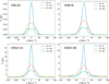 |
Fig. 8 Integrated line profile of the CO(1–0), CO(6–5), CO (12–11), and CO(15–14) transitions for the AGN torus simulation. The lines correspond to line profiles seen at different inclination angles, as the legend indicates. υ = 0 km s−1 corresponds the rest wavelength of each line transition. The line profiles are observed by observers located at a fiducial distance of 4.2 Mpc with a beam size of (32 pc)2. |
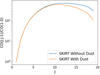 |
Fig. 9 CO SLEDs of the AGN torus model for an edge-on observer, calculated without dust (blue line) and with dust (orange line). Here, the beam size is (32 pc)2. |
5 Discussion and conclusions
Many codes are available in the astronomical literature for either dust radiative transfer or non-LTE line radiative transfer, but self-consistent 3D dust and non-LTE line radiative transfer codes have not been established. We introduced Monte-Carlo-based non-LTE line radiative transfer in the 3D dust radiative transfer code SKIRT. The result is a pure 3D Monte Carlo code that can self-consistently generate full spectra with continuum and molecular and atomic lines. The main goals of this paper are to investigate whether this approach can achieve an accuracy comparable to other codes and to assess how dust affects molecular emission lines.
Our first task was to validate the accuracy of the non-LTE line radiative transfer module in SKIRT. This was done using the van Zadelhoff et al. (2002) benchmark models. We compared our results with the reference results presented in this paper and the results obtained with the modern non-LTE line ray-tracing code MAGRITTE (De Ceuster et al. 2020). For the spherical problem 1a,b of van Zadelhoff et al. (2002), the level populations obtained by SKIRT agree with those obtained by MAGRITTE and the reference results as shown in Fig. 2. For benchmark problem 2a,b, for which we used a 3D grid in SKIRT, the SKIRT level populations show a very satisfactory agreement with the MAGRITTE ones with a relative difference of 20% maximum (Fig. 3). This accuracy is similar to the relative accuracy reached by other codes participating in the benchmark. For problem 1b we tested the dependence of the calculation accuracy on the number of photon packets and the optical depth of each cell. We find that the number of photon packets should be chosen such that Np > 800 × Ncell × Nline, and the optical depth of each cell should be chosen to be smaller than 70 to produce an accurate radial profile for the level populations. The requirement of optical depth is consistent with Camps & Baes (2018). The bottom line is that these benchmark tests validate SKIRT as a non-LTE line radiative transfer code.
Our second task consisted of demonstrating the new capabilities of the S KIRT code using a 3D hydrodynamic simulation and assessing how dust affects molecular emission lines. We performed a joint dust and non-LTE line radiative transfer simulation of the AGN torus simulation of Wada et al. (2016). As a result, we produced multiband images and SEDs with CO rotational lines. We find that the low-J CO emission traces the geometrically thick dusty molecular torus, whereas the higher-J CO lines originate from the gas with a high kinetic temperature, especially in the innermost region (see Fig. 6). The line profiles corresponding to these higher-J transitions show asymmetry due to turbulent gas in the torus (see Fig. 8). Furthermore, higher-J CO lines are slightly attenuated by surrounding cold dust when viewed edge-on. The fact that dust extinction affects even high-J rotational CO lines implies even stronger attenuation effects for atomic and molecular lines at the shorter wavelengths, such as H2 lines, OH rotational lines, and CO rovibrational lines. In future works, we will investigate the synthetic observations for molecular lines in the MIR and NIR wavelength range.
In addition, we note that the implementation of the non-LTE line module in SKIRT makes the radiative transfer code much more powerful and versatile than “just” a non-LTE line radiative transfer code. Indeed, thanks to the modular structure of the SKIRT code (Camps & Baes 2015, 2020), many of the features and capabilities built into the code over the last two decades are immediately available and can be combined with the new non-LTE line capabilities without the need to reinvent the wheel. In particular,
The non-LTE line radiative transfer capabilities can be combined with dust radiative transfer, resulting in self-consistent calculations of dust and line emission. This is particularly useful as dust emission can promote rotational or vibrational transitions. We note that the most commonly used dust models in the literature (e.g., Zubko et al. 2004; Draine & Li 2007; Jones et al. 2017) are built into SKIRT, and that the dust radiative transfer module is strongly optimized and thoroughly tested (Gordon et al. 2017);
SKIRT is fully 3D and optimized for radiative transfer on arbitrarily complex geometries, thanks to efficient grid traversal algorithms for hierarchical (Saftly et al. 2013, 2014) and unstructured grids (Camps et al. 2013). The new non-LTE line radiative transfer module can immediately use these grids. As a result, SKIRT is ideally suited to generate mock continuum and line observations for various types of hydrodynamical simulations, including grid-based, smoothed particle hydrodynamic, and moving-mesh simulations. On the other hand, the extensive library of built-in analytical geometries (Baes & Camps 2015) can be used to easily build phenomenological models for the interpretation of observations;
The SKIRT design is such that the user can easily set up multiple external radiation sources with arbitrary SEDs. Standard choices include the CMB or stellar populations with built-in or user-provided stellar population template libraries. CMB and stellar radiation can promote rotational and electronic transitions in atoms, respectively;
Non-LTE line radiative transfer calculations for different atoms and molecules (and dust) are performed simultaneously, and hence, we can consider the contamination of absorption and emission caused by other transition lines. Additionally, thanks to this feature, we can consider SKIRT to extend to post-processing calculations for chemical reactions in future works. We note that these calculations take significant computational costs currently;
SKIRT not only performs dust and non-LTE line radiative transfer but also Lyα resonant line radiative transfer (Camps et al. 2021) and X-ray radiative transfer (Vander Meulen et al. 2023). This offers the opportunity to explore a variety of observational tracers, covering the entire X-ray to radio regime, of the same system in a self-consistent manner.
The set of these features described above is unique to SKIRT. We argue that this code is ideal for generating mock observations including both continuum and atomic and molecular lines over a wide wavelength range. The applicability is not limited to a specific class of objects but covers various astronomical fields such as galaxies, star-forming regions, and AGNs. Therefore, our self-consistent dust and non-LTE line radiative transfer calculations in SKIRT can help in the interpretation of observational data from various telescopes such as Herschel, ALMA, and JWST, and we invite interested colleagues to apply it to their preferred astronomical objects.
Acknowledgements
Numerical computations were performed on the Cray XC50 at the Center for Computational Astrophysics, National Astronomical Observatory of Japan, and the SQUID at the Cybermedia Center, Osaka University as part of the HPCI system Research Project (hp220044). KM gratefully acknowledges the financial support of the Flemish Fund for Scientific Research (FWO-Vlaanderen) provided through grant number 1169822N. FDC is a postdoctoral research Fellow of the Research Foundation - Flanders, grant 1253223N. This work was supported by JSPS KAKENHI Grant Number 21H04496 (K.W. and T.N.), 23H05441 (T.N.), 19H05810, 20H00180, and 22K21349 (K.N.).
Appendix A General formalization of self-consistent non-LTE and dust radiative transfer
In this Appendix, we describe the formal equations that describe the self-consistent dust and non-LTE line radiative transfer calculation. The time-independent monochromatic radiative transfer equation is expressed as
 (A.1)
(A.1)
where I represents the specific intensity of the radiation, which is a function of position x, photon propagation direction n, and wavelength λ. αabs, αsca, and j are the absorption coefficient, the scattering coefficient, and the emissivity of the medium, and Φ is the scattering phase function. The emissivity has contributions from the gas, the dust, and any primary radiation source,
 (A.2)
(A.2)
The absorption coefficient has contributions from the gas and dust, whereas scattering is contributed only by dust as long as we consider the radiation in the UV-submillimeter wavelength range,
 (A.3)
(A.3)
 (A.4)
(A.4)
Gas media such as atoms, ionized atoms, and molecules have quantized energy levels composed of electronic, vibrational, and rotational levels. The transitions between two energy levels are responsible for the line emission and absorption of the photon at a particular wavelength. As a result, the absorption coefficients and the emissivity of the gas medium are related to the probability of the transitions and are given by
 (A.5)
(A.5)
 (A.6)
(A.6)
In the equations, Aul, Bul, and Blu are the Einstein coefficients, which are related by
 (A.7)
(A.7)
 (A.8)
(A.8)
with gu and gl the degeneracies of the upper and lower energy levels, respectively.
The absorption and scattering coefficients and the scattering phase function for the dust medium can be calculated when the sizes, chemical composition, and grain shapes are known. For spherical dust grains this can be done using Mie theory, for nonspherical grains more advanced methods need to be used (e.g., Voshchinnikov & Farafonov 1993; Draine & Flatau 1994; Mishchenko & Travis 1998; Vandenbroucke et al. 2020). The calculation of the dust emissivity depends on the absorption scattering coefficients and the temperature of the dust grains. If we assume that all dust grains are in equilibrium with the radiation field, the total emissivity of the dust medium is given by
 (A.9)
(A.9)
where the sum runs over all the different populations of dust grains, and the dust temperature Ti of the i’th population is determined from the balance equation
 (A.10)
Instead of the radiative equilibrium, we can also consider stochastic heating, in which the equilibrium temperature of each grain population is replaced by a temperature probability distribution (for details, see e.g. Camps et al. 2015).
Appendix B Collisional coefficients
The collisional de-excitation coefficients Cul depend on the number density of collisional partners np and the kinetic temperature Tkin. More specifically
 (B.1)
(B.1)
where Kul(Tkin) is the cross section of the collisional transition. The collisional de-excitation coefficients Cul and excitation coefficients Clu are related by
 (B.2)
(B.2)
References
- Aalto, S., Spaans, M., Wiedner, M. C., & Hüttemeister, S. 2007, A & A, 464, 193 [NASA ADS] [CrossRef] [EDP Sciences] [Google Scholar]
- Álvarez-Márquez, J., Labiano, A., Guillard, P., et al. 2023, A & A, 672, A108 [CrossRef] [EDP Sciences] [Google Scholar]
- Appleton, P. N., Guillard, P., Emonts, B., et al. 2023, ApJ, 951, 104 [NASA ADS] [CrossRef] [Google Scholar]
- Baes, M., & Camps, P. 2015, Astron. Comput., 12, 33 [NASA ADS] [CrossRef] [Google Scholar]
- Baes, M., Verstappen, J., De Looze, I., et al. 2011, ApJS, 196, 22 [Google Scholar]
- Baes, M., Gordon, K. D., Lunttila, T., et al. 2016, A & A, 590, A55 [CrossRef] [EDP Sciences] [Google Scholar]
- Baes, M., Camps, P., & Matsumoto, K. 2022, A & A, 666, A101 [NASA ADS] [CrossRef] [EDP Sciences] [Google Scholar]
- Bisbas, T. G., Bell, T. A., Viti, S., Yates, J., & Barlow, M. J. 2012, MNRAS, 427, 2100 [NASA ADS] [CrossRef] [Google Scholar]
- Bland-Hawthorn, J., & Gerhard, O. 2016, ARA & A, 54, 529 [NASA ADS] [CrossRef] [Google Scholar]
- Brinch, C., & Hogerheijde, M. R. 2010, A & A, 523, A25 [NASA ADS] [CrossRef] [EDP Sciences] [Google Scholar]
- Camps, P., & Baes, M. 2015, Astron. Comput., 9, 20 [Google Scholar]
- Camps, P., & Baes, M. 2018, ApJ, 861, 80 [NASA ADS] [CrossRef] [Google Scholar]
- Camps, P., & Baes, M. 2020, Astron. Comput., 31, 100381 [NASA ADS] [CrossRef] [Google Scholar]
- Camps, P., Baes, M., & Saftly, W. 2013, A & A, 560, A35 [CrossRef] [EDP Sciences] [Google Scholar]
- Camps, P., Misselt, K., Bianchi, S., et al. 2015, A & A, 580, A87 [NASA ADS] [CrossRef] [EDP Sciences] [Google Scholar]
- Camps, P., Trayford, J. W., Baes, M., et al. 2016, MNRAS, 462, 1057 [CrossRef] [Google Scholar]
- Camps, P., Behrens, C., Baes, M., Kapoor, A. U., & Grand, R. 2021, ApJ, 916, 39 [NASA ADS] [CrossRef] [Google Scholar]
- Camps, P., Kapoor, A. U., Trcka, A., et al. 2022, MNRAS, 512, 2728 [NASA ADS] [CrossRef] [Google Scholar]
- De Ceuster, F., Homan, W., Yates, J., et al. 2020, MNRAS, 492, 1812 [NASA ADS] [CrossRef] [Google Scholar]
- Draine, B. T., & Flatau, P. J. 1994, J. Opt. Soc. Am. A, 11, 1491 [NASA ADS] [CrossRef] [Google Scholar]
- Draine, B. T., & Li, A. 2007, ApJ, 657, 810 [CrossRef] [Google Scholar]
- Dullemond, C. P., & Turolla, R. 2000, A & A, 360, 1187 [NASA ADS] [Google Scholar]
- Dullemond, C. P., Juhasz, A., Pohl, A., et al. 2012, Astrophysics Source Code Library [record ascl:1282.815] [Google Scholar]
- Galliano, F., Galametz, M., & Jones, A. P. 2018, ARA & A, 56, 673 [NASA ADS] [CrossRef] [Google Scholar]
- Gatto, A., Walch, S., Naab, T., et al. 2017, MNRAS, 466, 1903 [NASA ADS] [CrossRef] [Google Scholar]
- Gebek, A., Baes, M., Diemer, B., et al. 2023, MNRAS, 521, 5645 [NASA ADS] [CrossRef] [Google Scholar]
- Gordon, K. D., Misselt, K. A., Witt, A. N., & Clayton, G. C. 2001, ApJ, 551, 269 [NASA ADS] [CrossRef] [Google Scholar]
- Gordon, K. D., Baes, M., Bianchi, S., et al. 2017, A & A, 603, A114 [NASA ADS] [CrossRef] [EDP Sciences] [Google Scholar]
- Granato, G. L., Ragone-Figueroa, C., Taverna, A., et al. 2021, MNRAS, 503, 511 [NASA ADS] [CrossRef] [Google Scholar]
- Hogerheijde, M. R., & van der Tak, F. F. S. 2000, A & A, 362, 697 [NASA ADS] [Google Scholar]
- Hsu, Y.-M., Hirashita, H., Lin, Y.-H., Camps, P., & Baes, M. 2023, MNRAS, 519, 2475 [Google Scholar]
- Imanishi, M., Nakanishi, K., & Izumi, T. 2016, ApJ, 825, 44 [Google Scholar]
- Imanishi, M., Nakanishi, K., & Izumi, T. 2017, ApJ, 849, 29 [NASA ADS] [CrossRef] [Google Scholar]
- Jones, A. P., Köhler, M., Ysard, N., Bocchio, M., & Verstraete, L. 2017, A & A, 602, A46 [NASA ADS] [CrossRef] [EDP Sciences] [Google Scholar]
- Juvela, M. 2019, A & A, 622, A79 [NASA ADS] [CrossRef] [EDP Sciences] [Google Scholar]
- Juvela, M. 2020, A & A, 644, A151 [CrossRef] [EDP Sciences] [Google Scholar]
- Kado-Fong, E., Kim, J.-G., Ostriker, E. C., & Kim, C.-G. 2020, ApJ, 897, 143 [NASA ADS] [CrossRef] [Google Scholar]
- Kapoor, A. U., Camps, P., Baes, M., et al. 2021, MNRAS, 506, 5703 [NASA ADS] [CrossRef] [Google Scholar]
- Keto, E., & Rybicki, G. 2010, ApJ, 716, 1315 [NASA ADS] [CrossRef] [Google Scholar]
- Kim, C.-G., & Ostriker, E. C. 2018, ApJ, 853, 173 [NASA ADS] [CrossRef] [Google Scholar]
- Kim, C.-G., Kim, J.-G., Gong, M., & Ostriker, E. C. 2023, ApJ, 946, 3 [NASA ADS] [CrossRef] [Google Scholar]
- Lahén, N., Naab, T., & Kauffmann, G. 2022, MNRAS, 514, 4560 [CrossRef] [Google Scholar]
- Leroy, A. K., Bolatto, A. D., Sandstrom, K., et al. 2023, ApJ, 944, L10 [NASA ADS] [CrossRef] [Google Scholar]
- Liu, D., Schinnerer, E., Cao, Y., et al. 2023, ApJ, 944, L19 [NASA ADS] [CrossRef] [Google Scholar]
- Mashian, N., Sturm, E., Sternberg, A., et al. 2015, ApJ, 802, 81 [Google Scholar]
- Matsumoto, K., Nakagawa, T., Wada, K., et al. 2022, ApJ, 934, 25 [NASA ADS] [CrossRef] [Google Scholar]
- Meidt, S. E., Rosolowsky, E., Sun, J., et al. 2023, ApJ, 944, L18 [CrossRef] [Google Scholar]
- Meijerink, R., & Spaans, M. 2005, A & A, 436, 397 [NASA ADS] [CrossRef] [EDP Sciences] [Google Scholar]
- Mishchenko, M., & Travis, L. D. 1998, J. Quant. Spec. Radiat. Transf., 60, 309 [NASA ADS] [CrossRef] [Google Scholar]
- Ng, K. C. 1974, J. Chem. Phys., 61, 2680 [NASA ADS] [CrossRef] [Google Scholar]
- Panuzzo, P., Rangwala, N., Rykala, A., et al. 2010, A & A, 518, A37 [Google Scholar]
- Rangwala, N., Maloney, P. R., Glenn, J., et al. 2011, ApJ, 743, 94 [NASA ADS] [CrossRef] [Google Scholar]
- Rathjen, T.-E., Naab, T., Girichidis, P., et al. 2021, MNRAS, 504, 1039 [NASA ADS] [CrossRef] [Google Scholar]
- Reissl, S., Wolf, S., & Brauer, R. 2016, A & A, 593, A87 [NASA ADS] [CrossRef] [EDP Sciences] [Google Scholar]
- Rich, J., Aalto, S., Evans, A. S., et al. 2023, ApJ, 944, L50 [CrossRef] [Google Scholar]
- Robitaille, T. P. 2011, A & A, 536, A79 [NASA ADS] [CrossRef] [EDP Sciences] [Google Scholar]
- Runco, J. N., Malkan, M. A., Fernández-Ontiveros, J. A., Spinoglio, L., & Pereira-Santaella, M. 2020, ApJ, 905, 57 [NASA ADS] [CrossRef] [Google Scholar]
- Rundle, D., Harries, T. J., Acreman, D. M., & Bate, M. R. 2010, MNRAS, 407, 986 [NASA ADS] [CrossRef] [Google Scholar]
- Saftly, W., Camps, P., Baes, M., et al. 2013, A & A, 554, A10 [CrossRef] [EDP Sciences] [Google Scholar]
- Saftly, W., Baes, M., & Camps, P. 2014, A & A, 561, A77 [CrossRef] [EDP Sciences] [Google Scholar]
- Schartmann, M., Wada, K., Prieto, M. A., Burkert, A., & Tristram, K. R. W. 2014, MNRAS, 445, 3878 [NASA ADS] [CrossRef] [Google Scholar]
- Schinnerer, E., Emsellem, E., Henshaw, J. D., et al. 2023, ApJ, 944, L15 [NASA ADS] [CrossRef] [Google Scholar]
- Schöier, F. L., van der Tak, F. F. S., van Dishoeck, E. F., & Black, J. H. 2005, A & A, 432, 369 [CrossRef] [EDP Sciences] [Google Scholar]
- Shu, F. H. 1977, ApJ, 214, 488 [Google Scholar]
- Stalevski, M., Fritz, J., Baes, M., Nakos, T., & Popovic, L. Č. 2012, MNRAS, 420, 2756 [NASA ADS] [CrossRef] [Google Scholar]
- Stalevski, M., González-Gaitán, S., Savic, Ð., et al. 2023, MNRAS, 519, 3237 [NASA ADS] [CrossRef] [Google Scholar]
- Steinacker, J., Baes, M., & Gordon, K. D. 2013, ARA & A, 51, 63 [NASA ADS] [CrossRef] [Google Scholar]
- Trayford, J. W., Camps, P., Theuns, T., et al. 2017, MNRAS, 470, 771 [NASA ADS] [CrossRef] [Google Scholar]
- Trcka, A., Baes, M., Camps, P., et al. 2022, MNRAS, 516, 3728 [CrossRef] [Google Scholar]
- Tristram, K. R. W., Impellizzeri, C. M. V., Zhang, Z.-Y., et al. 2022, A & A, 664, A142 [CrossRef] [EDP Sciences] [Google Scholar]
- Uzuo, T., Wada, K., Izumi, T., et al. 2021, ApJ, 915, 89 [NASA ADS] [CrossRef] [Google Scholar]
- Vandenbroucke, B., Baes, M., & Camps, P. 2020, AJ, 160, 55 [NASA ADS] [CrossRef] [Google Scholar]
- Vandenbroucke, B., Baes, M., Camps, P., et al. 2021, A & A, 653, A34 [NASA ADS] [CrossRef] [EDP Sciences] [Google Scholar]
- Vander Meulen, B., Camps, P., Stalevski, M., & Baes, M. 2023, A & A, 674, A123 [NASA ADS] [CrossRef] [EDP Sciences] [Google Scholar]
- van der Werf, P. P., Isaak, K. G., Meijerink, R., et al. 2010, A & A, 518, A42 [Google Scholar]
- van Zadelhoff, G. J., Dullemond, C. P., van der Tak, F. F. S., et al. 2002, A & A, 395, 373 [CrossRef] [EDP Sciences] [Google Scholar]
- Verstocken, S., Van De Putte, D., Camps, P., & Baes, M. 2017, Astron. Comput., 20, 16 [NASA ADS] [CrossRef] [Google Scholar]
- Voshchinnikov, N. V., & Farafonov, V. G. 1993, Ap & SS, 204, 19 [NASA ADS] [CrossRef] [Google Scholar]
- Wada, K. 2012, ApJ, 758, 66 [Google Scholar]
- Wada, K., Papadopoulos, P. P., & Spaans, M. 2009, ApJ, 702, 63 [NASA ADS] [CrossRef] [Google Scholar]
- Wada, K., Schartmann, M., & Meijerink, R. 2016, ApJ, 828, L19 [Google Scholar]
- Wada, K., Fukushige, R., Izumi, T., & Tomisaka, K. 2018, ApJ, 852, 88 [CrossRef] [Google Scholar]
- Wolfire, M. G., Vallini, L., & Chevance, M. 2022, ARA & A, 60, 247 [NASA ADS] [CrossRef] [Google Scholar]
- Zubko, V., Dwek, E., & Arendt, R. G. 2004, ApJS, 152, 211 [NASA ADS] [CrossRef] [Google Scholar]
The open-source SKIRT code is registered in the ASCL with the code entry ascl:1109.003 and is hosted at www.github.com/SKIRT/SKIRT9. Documentation and other information can be found at www.skirt.ugent.be
All Figures
|
Fig. 1 Execution flow of self-consistent dust and non-LTE line radiative transfer calculation in SKIRT and the schematic pictures of the radiative transfer of primary and secondary emission. Blue and red arrows represent primary and secondary emission, respectively. |
| In the text | |
|
Fig. 2 Comparison of the relative population at the upper level obtained with SKIRT (dots) and MAGRITTE (dashed lines) and the reference results of van Zadelhoff et al. (2002; gray solid lines) for benchmark problem 1a (blue lines) and 1b (green lines). The level population is normalized by the total number density. The differences of MAGRITTE and SKIRT results relative to the reference results are shown in the bottom panel. |
| In the text | |
|
Fig. 3 Comparison of the relative HCO+ level population for benchmark problem 2a (upper panels) and 2b (bottom panels) at J = 1 (left) and J = 4 (right) obtained with SKIRT (blue solid lines with dots) and MAGRITTE (yellow solid lines) and the reference results of van Zadelhoff et al. (2002; gray dashed lines). The level population is normalized by the total number density. The relative differences between the MAGRITTE and SKIRT results are shown in the lower subpanels. |
| In the text | |
|
Fig. 4 Convergence tests for benchmark problem 1b for calculations with different cell numbers, as indicated in the top right corner of the left panel. Left: relative populations at the upper level. Right: observed line profiles corresponding to a distance of 1 Mpc from the sphere’s center. In both cases, the relative differences between each simulation and the reference simulation with 400 cells are shown in the lower panels. |
| In the text | |
|
Fig. 5 Convergence tests for benchmark problem 1b for calculations with different photon packet numbers, as indicated in the top right corner of the left panel. Left: relative populations at the upper level. Right: observed line profiles corresponding to a distance of 1 Mpc from the sphere’s center. In both cases, the relative differences between each simulation and the reference simulation with 107 photon packets are shown in the bottom panels. |
| In the text | |
|
Fig. 6 Dust continuum images (first and second rows) and CO line emission maps (third and fourth rows) for the AGN torus model discussed in Sect. 4.1. Each image consists of 256 × 256 pixels with a pixel size of 0.125 pc. The images on the first and third rows are viewed face-on, and those on the second and fourth rows are viewed edge-on. |
| In the text | |
|
Fig. 7 Spectral energy distributions including CO rotational lines from J = 0 to J = 19 for the AGN torus simulation. The different lines correspond to SEDs seen at different inclination angles, as indicated in the legend. The observers are located at a fiducial distance of 4.2 Mpc, and a beam size of (32 pc)2 is used. |
| In the text | |
|
Fig. 8 Integrated line profile of the CO(1–0), CO(6–5), CO (12–11), and CO(15–14) transitions for the AGN torus simulation. The lines correspond to line profiles seen at different inclination angles, as the legend indicates. υ = 0 km s−1 corresponds the rest wavelength of each line transition. The line profiles are observed by observers located at a fiducial distance of 4.2 Mpc with a beam size of (32 pc)2. |
| In the text | |
|
Fig. 9 CO SLEDs of the AGN torus model for an edge-on observer, calculated without dust (blue line) and with dust (orange line). Here, the beam size is (32 pc)2. |
| In the text | |
Current usage metrics show cumulative count of Article Views (full-text article views including HTML views, PDF and ePub downloads, according to the available data) and Abstracts Views on Vision4Press platform.
Data correspond to usage on the plateform after 2015. The current usage metrics is available 48-96 hours after online publication and is updated daily on week days.
Initial download of the metrics may take a while.