| Issue |
A&A
Volume 643, November 2020
|
|
|---|---|---|
| Article Number | A21 | |
| Number of page(s) | 23 | |
| Section | Planets and planetary systems | |
| DOI | https://doi.org/10.1051/0004-6361/202039153 | |
| Published online | 27 October 2020 | |
Influences of protoplanet-induced three-dimensional gas flow on pebble accretion
II. Headwind regime
1
Department of Earth and Planetary Sciences, Tokyo Institute of Technology,
Ookayama, Meguro-ku,
Tokyo
152-8551,
Japan
e-mail: This email address is being protected from spambots. You need JavaScript enabled to view it.
2
Earth-Life Science Institute, Tokyo Institute of Technology,
Ookayama, Meguro-ku,
Tokyo
152-8550,
Japan
Received:
11
August
2020
Accepted:
14
September
2020
Abstract
Context. Pebble accretion is among the major theories of planet formation. Aerodynamically small particles, called pebbles, are highly affected by the gas flow. A growing planet embedded in a protoplanetary disk induces three-dimensional (3D) gas flow. In our previous work, Paper I, we focused on the shear regime of pebble accretion and investigated the influence of planet-induced gas flow on pebble accretion. In Paper I, we found that pebble accretion is inefficient in the planet-induced gas flow compared to that of the unperturbed flow, particularly when St ≲ 10−3, where St is the Stokes number.
Aims. Following on the findings of Paper I, we investigate the influence of planet-induced gas flow on pebble accretion. We did not consider the headwind of the gas in Paper I. Here, we extend our study to the headwind regime of pebble accretion.
Methods. Assuming a nonisothermal, inviscid sub-Keplerian gas disk, we performed 3D hydrodynamical simulations on the spherical polar grid hosting a planet with the dimensionless mass, m = RBondi∕H, located at its center, where RBondi and H are the Bondi radius and the disk scale height, respectively. We then numerically integrated the equation of motion for pebbles in 3D using hydrodynamical simulation data.
Results. We first divided the planet-induced gas flow into two regimes: flow-shear and flow-headwind. In the flow-shear regime, where the planet-induced gas flow has a vertically rotational symmetric structure, we find that the outcome is identical to what we obtained in Paper I. In the flow-headwind regime, the strong headwind of the gas breaks the symmetric structure of the planet-induced gas flow. In the flow-headwind regime, we find that the trajectories of pebbles with St ≲ 10−3 in the planet-induced gas flow differ significantly from those of the unperturbed flow. The recycling flow, where gas from the disk enters the gravitational sphere at low latitudes and exits at high latitudes, gathers pebbles around the planet. We derive the flow transition mass analytically, mt, flow, which discriminates between the flow-headwind and flow-shear regimes. From the relation between m, mt, flow and mt, peb, where mt, peb is the transition mass of the accretion regime of pebbles, we classify the results obtained in both Paper I and this study into four groups. In particular, only when the Stokes gas drag law is adopted and m < min(mt, peb, mt, flow), where the accretion and flow regime are both in the headwind regime, the accretion probability of pebbles with St ≲ 10−3 is enhanced in the planet-induced gas flow compared to that of the unperturbed flow.
Conclusions. Combining our results with the spacial variety of turbulence strength and pebble size in a disk, we conclude that the planet-induced gas flow still allows for pebble accretion in the early stage of planet formation. The suppression of pebble accretion due to the planet-induced gas flow occurs only in the late stage of planet formation, more specifically, in the inner region of the disk. This may be helpful for explaining the distribution of exoplanets and the architecture of the Solar System, both of which have small inner and large outer planets.
Key words: hydrodynamics / planets and satellites: formation / protoplanetary disks
© ESO 2020
1 Introduction
Recent hydrodynamical simulations have revealed that a planet embedded in a protoplanetary disk induces gas flow with a complex three-dimensional (3D) structure (Ormel et al. 2015; Fung et al. 2015, 2019; Lambrechts & Lega 2017; Cimerman et al. 2017; Kurokawa & Tanigawa 2018; Kuwahara et al. 2019; Béthune & Rafikov 2019). The anterior-posterior horseshoe flows extending in the orbital direction of the planet have a characteristic vertical structure that resembles a column. A substantial amount of gas from the disk enters the gravitational sphere of the planet (inflow) and exits (outflow), causing atmospheric recycling. Qualitatively, the 3D flow structure depends on the magnitude of the deviation of the speed of the gas from Keplerian rotation. In a Keplerian disk, the 3D planet-induced flow has a vertically rotational symmetric structure, but the symmetry is broken in a sub-Keplerian disk (Ormel et al. 2015; Kurokawa & Tanigawa 2018). The induced gas flow affects pebble accretion and may alter the accretion probability of pebbles. It has been seen that the accretion rate of small particles (~ 100 μm–1 mm) is reduced in the 2D planet-induced flow (Ormel 2013). Pebble accretion in the 3D planet-induced gas flow is shown to be more complicated. Popovas et al. (2018, 2019) incorporated pebbles into their hydrodynamical simulations and found that small particles (10 μm–1 cm) move away from the planet in the horseshoe flow, effectively avoiding accretion onto Earth- and Mars-sized planets.
Assuming a Keplerian disk, Kuwahara & Kurokawa (2020; hereafter Paper I) performed an orbital calculation of pebbles in 3D using hydrodynamical simulation data, finding that the 3D planet-induced gas flow affects pebble accretion significantly. In Paper I, planets of between three Mars masses and three Earth masses orbiting a solar-mass star at 1 au, ~ 0.3–3 M⊕, were considered, however the contribution of the headwind of the gas was not investigated by the authors. The shear regime of pebble accretion1 was only considered in Paper I, where the accretion radius for pebble accretion can be characterized by the size of the Hill radius and the approach velocity of pebbles is set by the shear velocity (Lambrechts & Johansen 2012; Ormel 2017; Johansen & Lambrechts 2017). When pebbles are aerodynamically small, those coming from within the vicinity of the planetary orbit move away from the planet along the horseshoe flows. The outflow of the gas at the midplane region deflects the pebble trajectories and inhibits small pebbles from accreting. The pebbles coming from a window between the horseshoe and the shear regions can accrete onto the planet. Thus, the width of the accretion window in the planet-induced gas flow is narrower than that of the unperturbed flow.
The accretion probability of pebbles, which is an important parameter in controlling the outcome of the pebble-driven planet formation model, is affected by the planet-induced gas flow. For a planet with ~ 0.3 M⊕, the accretion probability in the planet-induced gas flow is smaller than in of the unperturbed flow (Paper I). This is caused by the reduction of the width of the accretion window. When the planetary mass is larger than 0.3 M⊕, the accretion probability in the planet-induced gas flow is comparable to that of the unperturbed flow, except for cases when the pebbles are well-coupled to the gas. As the planetary mass increases, the width of the horseshoe region increases. Pebbles with high relative velocity accrete onto the planet. Thus, the reduction of the width of the accretion window and the increase in relative velocity cancel each other out.
In the protoplanetary disks, the disk gas rotates slower than Keplerian velocity due to the existence of the global pressure gradient. In Paper I, we focused on large planetary masses, ≳ 0.3 M⊕, for which the influence of the headwind on pebble accretion is negligible. In an early phase of the planetary growth, however, pebble accretion proceeds in the headwind regime, where the accretion radius for pebble accretion can be characterized by the size of the Bondi radius, and the approach velocity of pebbles is set by the sub-Keplerian speed (Lambrechts & Johansen 2012; Ormel 2017; Johansen & Lambrechts 2017). Furthermore, the influence of the 3D planet-induced gas flow whose vertically rotational symmetry is broken due to the strong headwind of the gas is still unclear. In Paper II, we extend the study initiated in Paper I to the headwind regime.
The structure of this paper is as follows. In Sect. 2, we describe the numerical method. In Sect. 3, we show the results obtained from a series of simulations. In Sect. 4, we discuss the implications for planet formation. We present a summary and conclusions in Sect. 5.
2 Methods
2.1 Model overview
Most of our methods are the same as those described in Paper I, apart from the investigation of the headwind of the gas. In the following sections, we describe the differences with Paper I and emphasize the key points of our model. Throughout all of our simulations, the length, times, velocities, and densities are normalized by the disk scale height, H, the reciprocal of the orbital frequency, Ω−1, the sound speed, cs, and the unperturbed gas density at the location of the planet, ρdisk, respectively.In this unit, the dimensionless planetary mass is given by
 (1)
(1)
where G is the gravitational constant, and Mpl is the mass of the planet. The Hill radius is given by  in this unit. We assume the minimum mass solar nebula (MMSN) model (Weidenschilling 1977a; Hayashi et al. 1985) when we convert the dimensionless quantities into dimensional ones.
We summarize the parameter spaces investigated in both Paper I and II in Fig. 1 and Table 1. In Sect. 3, we divide the results into four categories according to the classification of the flow and the accretion regimes (Fig. 1).
2.2 Three-dimensional hydrodynamical simulations
In this study, we performed nonisothermal 3D hydrodynamical simulations of the gas of the protoplanetary disk around a planet. Our simulations were performed in a spherical polar coordinate co-rotating with a planet with Athena++ (White et al. 2016; Stone et al. 2020). The computational domain ranges from 0 to π and 0 to 2π in the polar and azimuthal directions, respectively. Most of our methods of hydrodynamical simulations are the same as described in detail in Kurokawa & Tanigawa (2018), apart from the configuration of the size of the inner boundary. Since the initial condition is symmetrical in the vertical direction (z-direction), the structure of the planet-induced gas flow is symmetric with respect to the midplane. Our local simulations are not equipped to deal with the gap opening. We focus on low-mass planets (m ≤ 0.3) which do not shape the global pressure gradient in both Paper I and II (Fig. 1). We discuss the case of high-mass planets in Sect. 4.3.3.
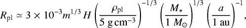
Kurokawa & Tanigawa (2018) fixed the size of the inner boundary for all of their simulations, but we varied it according to the mass of the planet. Following Paper I, assuming the density of the embedded planet ρpl = 5 g cm−3 leads to the physical radius of thecore, Rpl, as given by
 (2)
(2)
where M*, M⊙ and a are the stellar mass, the solar mass, and the orbital radius. We regard the size of rinn as being determined by Eq. (2), with a = 1 au2.
A planet is embedded in an inviscid gas disk and is orbiting around the central star at the distance, a, with the orbital frequency,  . The unperturbed gas velocity in the local frame
 (3)
(3)
From Eq. (3), the x-coordinate of the corotation radius for the gas can be described by
 (4)
(4)
The Mach number of the headwind of the gas is defined as
 (5)
(5)
where vhw is the headwind of the gas,
 (6)
(6)
where
 (7)
(7)
is a dimensionless quantity characterizing the pressure gradient of the disk gas, where P is the pressure of the gas and vK = aΩ is the Kepler velocity. The disk gas rotates slower than Keplerian velocity due to the existence of the global pressure gradient. The Mach number of the headwind is  in the MMSN model. In Paper I, we assumed
  for all of hydrodynamical simulations. In this study, we assume
  , and 0.1.
We list our parameter sets in Table 2. The range of the dimensionless planetary masses, m = 0.003–0.03, correspondsto planets of between three Moon masses and three Mars masses, Mpl = 0.036–0.36 M⊕, orbiting a solar-mass star at 1 au.
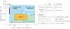 |
Fig. 1 Summary of parameter surveys in Paper I and II. The parameter spaces investigated in both Paper I and II are shown in redand yellow filled squares, respectively. The vertical and horizontal axes are the dimensionless planetary mass, m (Eq. (1)), and the Mach number of the headwind of the gas,
|

Parameters and regimes.
2.3 Three-dimensional orbital calculation of pebbles
We calculated the trajectories of pebbles influenced by the planet-induced gas flow in the frame co-rotating with the planet (Fig. 2). Most of our methods for carrying out orbital calculations of pebbles are the same as in Paper I, apart from the analysis of the headwind of the gas. In our co-rotating frame, the x- and y-components of the initial velocity of pebbles are given by the drift equations (Weidenschilling 1977a; Nakagawa et al. 1986):

From Eq. (9), the x-coordinate of the corotation radius for the pebble can be described by
 (10)
(10)
where St is the dimensionless stopping time of a pebble, called the Stokes number,
 (11)
(11)
We assume St = 10−4–100. The stopping time of the particle is described by
![Mathematical equation: \begin{equation*} t_{\textrm{stop}}=\left\{ \begin{array}{@{}ll} \displaystyle\frac{\rho_{\bullet}s}{\rho_{\textrm{g}}c_{\textrm{s}}}, & \displaystyle \left(\text{Epstein regime}: s\leq\frac{9}{4}\lambda\right),\hspace*{5.1pc}\hfil(12)\nonumber\\[6pt] \displaystyle\frac{4\rho_{\bullet}s^{2}}{9\rho_{\textrm{g}}c_{\textrm{s}}\lambda}, &\displaystyle \left(\text{Stokes regime}: s\geq\frac{9}{4}\lambda\right),\hspace*{5.4pc}\hfil(13)\nonumber\end{array}\right. \end{equation*}](/articles/aa/full_html/2020/11/aa39153-20/aa39153-20-eq16.png)
where ρ• is the internal density of the pebble, s is the radius of the pebble, and λ is the mean free path of the gas,  with
with  , mH, and σmol being the mean molecular weight,
  , the mass of the proton, and the molecular collision cross-section, σmol = 2 × 10⁻¹⁵ cm2 (Chapman & Cowling 1970; Weidenschilling 1977b; Nakagawa et al. 1986). The gas density at the midplane is given by
  , where Σg is the gas surface density,
  . The radius of a pebble is fixed in a orbital simulation, and the Stokes number is defined with the unperturbed gas density.
We performed orbital calculations for three different settings. First, the unperturbed flow case, hereafter, the UP-mXX-hwYY case3, where we adopt unperturbed sub-Keplerian shear flow where the gas density is uniform. The XX and YY denote the adopted values of the planetary mass and the Mach number of the headwind. We omit -mXX or -hwYY when we do not specify the planetary mass or the Mach number of the headwind. Since the gas density around the planet is constant, there is no difference between the Stokes and the Epstein regimes in the case of unperturbed flow. Second, the planet-induced flow case in the Epstein regime (Eq. (12)); hereafter the PI-Epstein-mXX-hwYY case. Third, the planet-induced flow case in the Stokes regime (Eq. (13)); hereafter the PI-Stokes-mXX-hwYY case.
In all of our hydrodynamical simulations, a hydrostatic envelope is formed around the planet. The density structure of an envelope is determined by the hydrostatic equilibrium with the gravity of the planet. The gas density increases significantly in the vicinity of the planet in the PI cases. Since the Stokes number in the Epstein regime is proportional to the reciprocal of the gas density, the effective Stokes number decreases as the gas density increases4. For the latter two cases, we switched the gas flow from unperturbed sub-Keplerian to planet-induced gas flow obtained by hydrodynamical simulations at r = rout. We used the final state of the hydro-simulations data (t = tend), where the flow field seems to have reached a steady state. We interpolated the gas velocity using the bilinear interpolation method (see Appendix B in Paper I).
When m = 0.01 and 0.03, we find thatthe horseshoe flow forms unexpected vortices, which influence the pebble trajectories. The origin of these vortices is unknown, but it is likely to be a numerical artifact due to the spherical polar coordinates centered at the planet, in which the resolution becomes too low to resolve the horseshoe flow far from the planet when the assumed planet mass is small. To avoid the effects of the vortices, we use the same method as in Paper I, only in our case, we use the limited part of the calculation domain, r ≤ 0.6rout.
Hydrodynamical simulations.
 |
Fig. 2 Schematic picture of an orbital calculation of pebbles. A planet is located at the origin of the co-rotational frame. The dashed line represents the outer boundary of the hydrodynamical simulations. The starting point of orbital calculation is beyond the outer boundary of hydrodynamical simulations. Its y-component is fixed at 40 RHill (Ida & Nakazawa 1989). The x- and z-coordinates of the starting point of pebbles, xs and zs, are the parameters. The gas velocity is assumed to be the speed of the sub-Keplerian shear both inside and outside of rout in the shear flow case of the unperturbed flow (UP-mXX-hwYY case), but is switchedto the gas velocity obtained from the hydrodynamical simulations within rout in the planet-induced flow case in the Epstein regime (PI-Epstein-mXX-hwYY case), and in the Stokes regime (PI-Stokes-mXX-hwYY case). |
2.4 Calculation of accretion probability of pebbles
2.4.1 Width of the accretion window and accretion cross-section
We defined the width of the accretion window as
 (14)
(14)
where xmax,i(z) and xmin,i(z) are the maximum and minimum values of the x-component of the starting point of accreted pebbles at a certain height. The subscript, i, denotes the number of the accretion window. When we include the headwind of the gas, the accretion of pebbles occurs asymmetrically with respect to the corotation radius for the pebble. In the unperturbed flow, the width of the accretion window is identical to the maximum impact parameter of accreted pebbles, bx, when St < 1 as xmin,i(z) = 0 (Eqs. (A.1) and (A.2)). Using this definition, we defined the accretion cross-section as
 (15)
(15)
where zmax,i and zmin,i are the maximum and the minimum value of the z-component of the starting point of accreted pebbles. We reduced the spatial intervals stepwise near the edge of the accretion window and determined xmax,i(z) and xmin,i(z) with sufficient accuracy. The initial spatial intervals are  in the x and z directions, where bx, hw and bx, sh are the maximum impact parameter of accreted pebbles in the unperturbed flow (Eqs. (A.1) and (A.2)).
2.4.2 Accretion probability
We define the accretion probability of pebbles as
 (16)
(16)
where Ṁp is the accretion rate of pebbles onto a protoplanet and Ṁdisk is the radial inward mass flux of pebbles in the gas disk described by
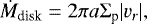 (17)
(17)
where Σp is the surface density of pebbles. The density distribution of pebbles is described by
![Mathematical equation: \begin{align*} \rho_{\textrm{p}}(z)=\frac{\Sigma_{\textrm{p}}}{\sqrt{2\pi}H_{\textrm{p}}}\exp\left[-\frac{1}{2}\left(\frac{z}{H_{\textrm{p}}}\right)^{2}\right],\end{align*}](/articles/aa/full_html/2020/11/aa39153-20/aa39153-20-eq27.png) (18)
(18)
where Hp is the scale height of pebbles (Dubrulle et al. 1995; Cuzzi et al. 1993; Youdin & Lithwick 2007):
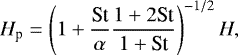 (19)
(19)
where α is the dimensionless turbulent parameter in the disk introduced by Shakura & Sunyaev (1973). Our calculation of accretion probability assumes that pebbles have a vertical distribution given by Eq. (18). This approach neglects the effect of random motion of individual particles (see, Paper I, for the discussion). The accretion rate of pebbles, Ṁp, is divided into two formulas:
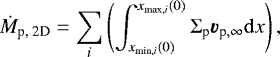 (20)
(20)
in the 2D case and
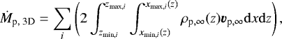 (21)
(21)
in the 3D case.
In order to account for the accretion from z < 0, we multiply Eq. (21) by two. The accretion probabilities for a fixed dimensionless planetary mass, m, in both 2D and 3D do not depend on the orbital radius, a (see Appendix C in Paper I). Following Paper I, we fixed the inward pebble mass flux as Ṁdisk = 102 M⊕ Myr−1, which is consistent with the typical value of the pebble flux used in a previous study (Lambrechts et al. 2019).
3 Results
3.1 Results overview
The main objective of this study is to clarify the influence of the planet-induced gas flow on pebble accretion. In Sect. 3.2, we show the characteristic 3D structure of the planet-induced gas flow field obtained by 3D hydrodynamical simulations. In Sect. 3.4, we show the results of our orbital calculations. Section 3.5 shows the dependence of the accretion probability of pebbles on the planetary mass, the Stokes number, and the Mach number of the headwind of the gas.
In Sects. 3.4 and 3.5, we divide the results into four categories according to the classification of the flow (Sects. 3.3 and 4.1) and the accretion (Appendix A) regimes as shown in Fig. 1. The UP simulations were performed as control experiments in order to understand the influences of planet’s gravity by comparing the results with those of the planet-induced flow (PI) and, thus, UP cases are not categorized in any categories in Fig. 1. The Keplerian and sub-Keplerian disk classification corresponds to different input parameter spaces ( and
and  ) and, thus, they do not correspond to four categories of the output results. Since the gas drag (Epstein and Stokes) regimes are determined independently of the planetary mass and the Mach number of the headwind, we do not use them in four categories in Fig. 1. In other words, all four categories should have two sub-categories for gas drag regimes.
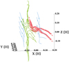 |
Fig. 3 Streamlines of 3D planet-induced gas flow around the planet. The result obtained from m003-hw01 at t = 50. The red, green, and blue solid lines are the recycling streamlines, the horseshoe streamlines, and the Keplerian shear streamlines, respectively. For the recycling streamlines, we only plot the streamlines which pass over the surface of the Bondi sphere. The arrows represent the direction of the gas flow. |
3.2 Three-dimensional planet-induced gas flow
When  , the planet-induced gas flow has a rotational symmetric structure with respect to the z-axis (see Fig. 2 of Paper I). The nonzero headwind of the gas breaks the symmetry of the planet-induced gas flow (Ormel et al. 2015; Kurokawa & Tanigawa 2018). Figure 3 shows the 3D flow structure around an embedded planet in an endmember case,
  . Gas flow shows three types of streamlines. (1) The planetary envelope is exposed to the headwind of the gas. Gas from the disk enters the Bondi sphere at low latitudes (inflow) and exits at high latitudes (outflow: the red lines of Fig. 3). This recycling flow passes the planet, tracing the surface of the isolated envelope whose size is ≲ 0.5 RBondi (Kurokawa & Tanigawa 2018). The detailed structure of the recycling streamlines is shown in Fig. 4. (2) The horseshoe streamlines lie inside the planetary orbit (the green lines of Fig. 3). (3) The Keplerian shear flow extends inside the horseshoe flow and outside the planetary orbit (the blue lines of Fig. 3).
3.3 Classification of the planet-induced gas flow
We introduce the classification of the planet-induced gas flow to clarify its influence on pebble accretion. Figure 5 shows how the structure at the midplane around an embedded planet depends upon the Mach number. When  and 0.03, a slight rotational symmetry remains with respect to the z-axis (Figs. 5a and b). The horseshoe streamlines still lie near the planetary orbit, which protects the planetary envelope from the headwind of the gas. The 3D structure of the planet-induced gas flow is similar to that found when
  , where the inflow occurs at high latitudes of the Bondi sphere and the outflow occurs at the midplane region of the disk (see Fig. 2 of Paper I). We refer to such a case as the flow-shear regime. All of the results shown in Paper I can be considered to be results in the flow-shear regime.
As the Mach number of the headwind of the gas increases, the horseshoe streamlines move to the negative direction in the x-axis. This is because the corotation radius for the gas moves toward the negative direction of the x-axis. When  , the horseshoe streamlines lie inside thex-coordinate of the Bondiradius (Fig. 5c). The planetary envelope is exposed to the headwind. Within the Bondi radius, the azimuthal velocity of the gas is low (Fig. 6). The envelope is pressure supported. The 3D structure of the planet-induced gas flow differs from that which can be seen in the flow-shear regime. We refer to such a case as the flow-headwind regime. Based on a series of hydrodynamical simulations, we classified the planet-induced gas flow into the flow-shear and the flow-headwind regimes, which are listed in Table 2. We discuss the transition from the flow-shear to the flow-headwind regime in Sect. 4.1.
3.4 Orbital calculations
3.4.1 Pebble accretion in 2D
We first focus on the 2D limit of pebble accretion in the Stokes regime, that is, where all of the pebbles have settled in the midplane of the disk and the Stokes number of pebbles does not depend on the gas density. Figure 7 shows the trajectories of pebbles at the midplane of the disk. We compared the results of UP-m001-hw01 case and PI-Stokes-m001-hw01 case. When the Stokes number is larger than St ≥ 10−1, the trajectories of pebbles and the width of the accretion window are similar (Figs. 7c, d, g, and h). When the Stokes number is smaller than St ≤ 10−2, the trajectories of pebbles near the planetary orbit are deflected by the recycling flow (Figs. 7a, b, e, and f). Since the planet chiefly perturbs the surrounding disk gas at a scale that is typically the smaller of the two when comparing the Bondi and Hill radii (Kuwahara et al. 2019), the difference between UP-m001-hw01 and PI-Stokes-m001-hw01 cases can be seen in the region close to the planet. In particular, the accretion window is wider in the planet-induced gas flow than in the unperturbed flow when St = 10−3 (Figs. 7a and e). This is in contrast to the conclusion in Paper I, where the width of the accretion window in the planet-induced gas flow in the flow-shear regime becomes narrower than those of the unperturbed shear flow (see Fig. 3 of Paper I). The difference is caused by the headwind of the gas.
Figure 8 compares the results between UP-m003-hw01 and PI-Stokes-m003-hw01 cases. This figure shows the significant difference of the trajectories of pebbles with St = 10−4. In the case of PI-Stokes-m003-hw01, the recycling flow deflects the trajectories of pebbles. This deflection is not found in 2D simulations (Ormel 2013), but it appears in the 3D ones. The pebbles are jammed outside the planetary orbit. Some of the pebbles from inside the planetary orbit move away from the planet along the horseshoe flow. In the flow-shear regime, the horseshoe flow that lies near the planetary orbit reduces the width of the accretion window (Paper I). The outflow occurs in the second and fourth quadrants of the x-y plane (Kuwahara et al. 2019). On the other hand, in the flow headwind regime, since the horseshoe flow shifts significantly to the negative direction in the x-axis, it does not suppress pebble accretion. The outflow occurs only in the fourth quadrant of the x-y plane. The accretion of pebbles coming from the region where y > 0 is not inhibited. Pebbles are susceptible to becoming entangled in the recycling flow. This leads to an increase in the time taken for pebbles to pass the Bondi radius of the planet (see Sect. 3.4.3).
In the PI-Epstein case, the shape of trajectories of pebbles does not differ significantly from that in the PI-Stokes case. However, the width of the accretion window, the accretion cross-section, and the accretion probability in the PI-Epstein case do not match those in the PI-Stokes case (see Sect. 3.5).
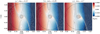 |
Fig. 5 Flow structure around a planet with m = 0.03 at the midplane of the disk. Panel a: result obtained from m003-hw001 at t = 50. Panel b: result obtained from m003-hw003 at t = 50. Panel c: result obtained from m003-hw01 at t = 50. Color contour represents the flow speed in the y-direction. The verticaland horizontal axis are normalized by the scale height of the disk. The solid lines correspond to the specific streamlines.The dotted and dashed lines are the Bondi and Hill radius of the planet, respectively. We note that the length of the arrows does not scale with the flow speed. |
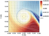 |
Fig. 6 Enlarged view of Fig. 5c, but the color contour represents the flow speed in the azimuthal direction. |
3.4.2 Pebble accretion in 3D
Next, we focus on the 3D behavior of pebble accretion in the Stokes regime. Figure 9 shows the 3D trajectories of pebbles with St = 10−4. This figure compares the results between UP-m003-hw01 and PI-Stokes-m003-hw01 cases. Since the gravity of the planet acting on the pebbles becomes weaker at high altitudes, pebbles do not accrete onto the planet in the UP-m003-hw01 case (Fig. 9a). On the other hand, even if pebbles come from high altitudes (zs ~ RBondi), they accreteonto the planet in the PI-Stokes-m003-hw01 case (Fig. 9b). This is caused by the recycling flow in the vicinity of the planet. The typical scale of the recycling flow is the size of the Bondi radius (Fig. 4). In the flow-shear regime, since the horseshoe flow has a vertical structure like a column, pebbles coming from high altitudes move away from the planet near the planetary orbit. In the flow-headwind regime, the horseshoe flow does not inhibit pebble accretion. When pebbles that come from high altitudes reach the vicinity of the planet, a fraction of those that reside in z ≲ RBondi become entangled in the recycling flow. This causes an increase in the time it takes for pebbles to cross the Bondi radius (see Sect. 3.4.3). Pebbles can accrete onto the planet even when they come from high altitudes.
3.4.3 Increase in the Bondi crossing time of pebbles
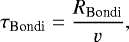
Figures 10 and 11 show the trajectories of pebbles that are projected on the x-y plane, and the relative velocity of pebbles to the planet as a function of the distance from the planet, r. We selected the pebbles passing near the Bondi region. In the UP cases, even when the pebbles pass near the Bondi sphere, their relative velocity does not change unless they reach the region very close to the planet, r ≲ 0.1RBondi (Figs. 10a and 11a). In the PI cases, significant velocity fluctuation can be seen when the pebbles enter the Bondi sphere (Figs. 10b and 11b). We define the Bondi crossing time of pebbles as
 (22)
(22)
where v is the relative velocity of pebbles to the planet. From Figs. 10b and 11b, we can see that the relative velocity of pebbles is reduced by an order of magnitude when they enter the Bondi sphere. This leads to an increase in the Bondi crossing time of pebbles by an order of magnitude. Just before accreting onto the planet, the relative velocity of pebbles to the planet reaches terminal velocity in both UP and PI cases, which is determined by the force balance between the gas drag and the gravity of the planet acting on the pebble:
 (23)
(23)
Within the Bondi sphere, the gas density increases significantly to maintain hydrostatic equilibrium. The velocity of the gas is reduced, and then a long-stagnant gas flow field is formed within the Bondi region (Fig. 6). Once the pebbles enter the Bondi sphere and become entangled in the recycling flow, the strong gas drag force reduces their relative velocity.
In the flow-headwind regime, the horseshoe flow shifts significantly to the negative direction in the x-axis and the outflow occurs only in the fourth quadrant in the x-y plane. Pebbles coming from the region where y > 0 and passing near the planetary orbit are susceptible to becoming entangled in the recycling flow. Thus, pebble accretion is enhanced in the planet-induced gas flow.
 |
Fig. 7 Trajectories of pebbles in UP-m001-hw01 case (top) and PI-Stokes-m001-hw01 case (bottom) with different Stokes numbers at the midplane of the disk. We set zs = 0 for all cases. The red and blue solid lines correspond to the trajectories of pebbles which accreted and did not accrete onto the planet, respectively. The dashed circles show the Hill radius of the planet. The sizes of the Hill and Bondi radii are 0.15 [H] and 0.01 [H]. The black dot at the center of each panel denotes the position of the planet. The interval of pebbles at their initial locations is 0.05 [H]. The regimes of pebble accretion and the planet-induced gas flow are determined by Eqs. (A.4) and (28). |
3.5 Accretion probability of pebbles
3.5.1 Width of the accretion window and accretion cross-section
Figure 12 shows the changes of the width of the accretion window in the midplane region as a function of the Stokes number for different planetary masses and the Mach numbers. We first focus on the left column of Fig. 12, where we compare the results between the UP case and PI-Stokes cases. As seen across all panels in the left column of Fig. 12, the accretion window is wider in the planet-induced gas flow than in the unperturbed flow when the accretion and flow regime are both in the headwind regime (filled circles in Figs. 12a, c, and e). This is one of the most important findings of our study. When the accretion occurs in the shear regime and the planet-induced gas flow is in the flow-headwind regime (filled squares in Figs. 12a, c, and e), the widths of the accretion window in the UP and PI-Stokes cases match each other.
When the planet-induced gas flow is in the flow-shear regime (open circles and squares in Figs. 12a, c, and e), the trend can be explained by the conclusion of Paper I. In the flow-shear regime, since the horseshoe flow lies near the planetary orbit, pebbles coming from the narrow region between the horseshoe and the shear regions can accrete onto the planet. This causes the reduction of the width of the accretion window. The width of the accretion window is not a simple increasing function of the Stokes number (e.g., Figs. 12a and b). As pebbles continue to drift inward as they approach the planet, the accretion of pebbles from y < 0 does not occur at all in some cases, leading to the complicated dependence of accretion width on St (see Fig. 13).
When m = 0.01 and 0.03, the significant influence of the planet-induced gas flow can be seen for the pebbles with St ≲ 10−2. When m = 0.003, the influence of the planet-induced gas flow is weak compared to the cases of m ≥ 0.01. The size of the perturbed region is determined by the gravity of the planet (Kuwahara et al. 2019). Thus the influence of the planet-induced gas flow on pebble accretion becomes weak as the planetary mass decreases.
Next, we focus on the right column of Fig. 12, where we compare the results between the UP case and PI-Epstein case. In contrast to the result shown in the left column of Fig. 12, the width of the accretion window decreases in the planet-induced gas flow when the accretion and flow regime are both in the headwind regime (the filled circles in Figs. 12b, d, and f). Since the gas density is higher around the planet due to its gravity, the effective Stokes number decreases as the pebble approaches the planet. This causes significant reduction in the width of the accretion window, particularly for St ≲ 10−3. When the accretion occurs in the shear regime and the planet-induced gas flow is in the flow-headwind regime (the filled squares in Figs. 12b, d, and f), or when the planet-induced gas flow is in the flow-shear regime (the open circles and squares in Figs. 12b, d, and f), the results are similar to those in the PI-Stokes case.
Figures 13 and 14 show the accretion windows of pebbles in the UP-m001-hw003 case, PI-Stokes-m001-hw003 case, UP-m001-hw01 case, and in the PI-Stokes-m001-hw01 case. We plotted all of the accretion windows in Figs. 13 and 145. In Fig. 13, there are one or two accretion windows. The accretion window has an asymmetric shape with respect to the x = xpeb, cor plane. This is caused by the radial drift of pebbles. For the range of the Stokes numbers considered here, the speed of the inward drift increases with the Stokes number and has a peak at St = 100 for a fixed Mach number (Eq. (8)).
We first focus on the top panel of Fig. 13 (UP-m001-hw003 case). Pebbles with St ≥ 10−2 coming from the region where x < xpeb, cor experience fast radial drift and do not accrete onto the planet. When St = 10−3, accretion from the region where x < xpeb, cor can be seen due to the slow radial drift of pebbles (Fig. 13b). When St = 10−4, the radial drift of pebbles is limited, but the x-coordinate of the pebble corotation radius is larger than the maximum impact parameter of the accreted pebbles, |xpeb, cor| > bhw. Thus, accretion occurs only in the region where x > xpeb,cor. The differences in the number of accretion windows for the combination of  , and m lead to the complex behavior with regard to the width of the accretion window (Fig. 12).
In the bottom panels of Fig. 13 (PI-Stokes-m001-hw003 case), the shape of the accretion windows is similar to that of the UP-m001-hw003 case when St ≥ 10−1. When St = 10−2, the accretion occurs in the region where x < xpeb, cor, which is not found in the UP-m001-hw003 case. When St ≤ 10−3, the height of the accretion window in x < xpeb, cor is larger than in x > xpeb, cor. The 3D structure of the planet-induced gas flow is almost rotationally symmetric, but the polar inflow shifts slightly to the negative direction in the x-axis as well as the horseshoe flow. This promotes the accretion of pebbles from high altitudes in the region where x < xpeb, cor.
Strong headwind causes fast radial drift. The accretion occurs only in the region where x > xpeb. cor in Fig. 14. In the flow-headwind regime, pebbles can accrete onto the planet even if they come from high altitudes (Fig. 9). The width of the accretion window in the planet-induced gas flow is larger than that of the unperturbed flow (Fig. 12). These findings can also be seen in Fig. 14. We find that the accretion window expands at the same location (Figs. 14a and f). When the pebbles are well-coupled to the gas (St = 10−4), the vertical scale of the accretion window is identical to the scale of the recycling flow (z ~ RBondi). This is in contrast to the results in Paper I, where the outflow in the midplane region and the vertical structure of the horseshoe flow inhibitspebble accretion in the flow-shear regime.
Figure 15 shows the differences between the integrated accretion cross-section in the UP, PI-Stokes, and PI-Eptein cases, as well as the dependence on the planetary mass and the Mach number. We first focus on the left column of Fig. 15. As shown in Fig. 14, we confirmed that the accretion cross-section is larger in the planet-induced gas flow than in the unperturbed flow when the accretion and flow regime are both in the headwind regime (filled circles in Figs. 15a, c, and e). This is an important finding, as is the increase in the width of the accretion window in the flow-headwind regime. When the accretion occurs in the shear regime and the planet-induced gas flow is in the flow-headwind regime (filled squares in Figs. 15a, c, and e), the accretion cross-sections in the UP and PI-Stokes cases match each other. When the planet-induced gas flow is in the flow-shear regime (the open circles and squares in Figs. 15a, c, and e), the trend can be explained by the conclusion drawn in Paper I. In the flow-shear regime, since the horseshoe flow lies near the planetary orbit, pebbles coming from the narrow region between the horseshoe and the shear regions can accrete onto the planet. This causes a reduction of the accretion cross-section in the planet-induced gas flow. Similarly to the width of the accretion window, the significant influence of the planet-induced gas flow can be seen for the pebbles with St ≲ 10−2 when m = 0.01 and 0.03, but it becomes weak when m = 0.003.
Next, we focus on the right column of Fig. 15, where we compare the results between the UP case and PI-Epstein case. In contrast to the result shown in the left column of Fig. 15, the accretion cross-section is smaller in the planet-induced gas flow than in the unperturbed flow when the accretion and flow regime are both in the headwind regime, except when m = 0.03 (the filled circles in Figs. 15b and d). Since the gas density is higher around the planet due to its gravity, the effective Stokes number decreases as the pebble approaches the planet. This causes significant reduction in the width of the accretion window, in particular for St ≲ 10−3. When the accretion occurs in the shear regime and the planet-induced gas flow is in the flow-headwind regime (the filled squares in Figs. 15b, d, and f), or when the planet-induced gas flow is in the flow-shear regime (the open circles and squares in Figs. 15b, d, and f), the results are similar to those in the PI-Stokes case.
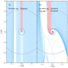 |
Fig. 8 Trajectories of pebbles in UP-m003-hw01 case (left panel) and PI-Stokes-m003-hw01 case (right panel) with St = 10−4 at the midplane of the disk. We set zs = 0. The red and blue solid lines correspond to the trajectories of pebbles which accreted and did not accrete onto the planet, respectively. The dotted-dashed and dashed circles show the Bondi and the Hill radius of the planet, respectively. The sizes of the Bondi radius and the Hill radius are 0.03 [H] and 0.22 [H]. The black dots at the center of each panel denote the position of the planet. The interval of pebbles at their initial locations is 0.003 [H]. |
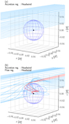 |
Fig. 9 Trajectories of pebbles with St = 10−4 in UP-m003-hw01 case (top) and PI-Stokes-m003-hw01 case (bottom). The height of the initial position of the pebbles is zs = 0.03 [H]. The red and blue solid lines correspond to the trajectories of pebbles which accreted and did not accrete onto the planet, respectively. The black dots at the center of each panel denote the position of the planet. The sphere around the planet represents the Bondi radius of the planet. We only plot the trajectories within the region where r < 2RHill. The interval of pebbles at their initial locations is 0.01 [H]. |
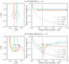 |
Fig. 10 Trajectories (left) and the relative velocity of pebbles to the planet (right) with St = 10−4. Panel a: results obtained from UP-m003- hw01 case. Panel b: results obtained from PI-Stokes-m003-hw01 case. We set zs = 0 [H]. Different colors correspond to different xs as indicated in figure legends. The dots on the solid lines mark intervals of Ω−1. The black dot and the dotted-dashed circle in the left column show the position of the planet and the Bondi radius of the planet. The vertical solid and dashed lines in the right column show the size of the Bondi radius and the terminal velocity of pebbles (Eq. (23)). |
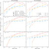 |
Fig. 12 Width of the accretion window in the midplane, wacc(0), as a function of the Stokes number in the UP (dotted lines), PI-Stokes (solid lines), and the PI-Epstein cases (dashed lines). Left column: compares the results between UP and PI-Stokes cases. Right column: compares the results between UP and PI-Epstein cases. The masses of the planet from top to bottom rows: m = 0.003, 0.01, and 0.03, respectively. Colors indicate the Mach number of the headwind of the gas:
|


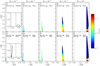 |
Fig. 13 Accretion window with the different Stokes numbers in the UP-m001-hw003 (top) and the PI-Stokes-m001-hw003 cases (bottom). We assume α = 10−3 and the dust-to-gas ratio equal to 10−2. Color represents the density of the pebbles expressed by Eq. (18) normalized by the gas density. The vertical dashed lines correspond to the corotation radius for pebbles (Eq. (10)). The two panels in panelsa and e show the enlarged outlines of accretion windows. We note that the color contour is saturated for ρp ≲ 10−3. |
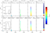 |
Fig. 14 Same as Fig. 13, but in the UP-m001-hw01 case (top) and the PI-Stokes-m001-hw01 case (bottom). |
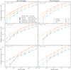 |
Fig. 15 Accretion cross-section, Aacc, as a function of the Stokes number in UP (dotted lines), PI-Stokes (solid lines), and PI-Epstein cases (dashed lines). Left column: compares the results between UP and PI-Stokes cases. Right column: compares the results between UP and PI-Epstein cases. The masses of the planet from top to bottom rows: m = 0.003, 0.01, and 0.03, respectively. Colors indicate the Mach number of the headwind of the gas:
|


3.5.2 Accretion probability
Figure 16 shows the 2D accretion rate and accretion probability as a function of the Stokes number for the different planetary masses and the Mach numbers. The explanation in Fig. 12 can be applied to this figure. The location of the accretion window does not change in the planet-induced gas flow in the flow-headwind regime. Figure 16 reflects the results of Fig. 12. In the left column, where we compare the results between the UP case and PI-Stokes case, the 2D accretion probability is larger in the planet-induced gas flow than in the unperturbed flow when the accretion and flow regime are both in the headwind regime (the filled circles in Figs. 16a, c, and e). This is because the width of the accretion window is larger in the planet-induced gas flow than in the unpertubed flow. We find that the enhancement of the 2D accretion probability in the PI-Stokes becomes more significant as the planetary mass increases. We note that when m = 0.03 and  , the accretion probability of pebbles with St = 10−4 approaches unity (Fig. 16e). Because we do not trace the pebble trajectory in the global disk, the accretion of slowly drifting pebbles might be double-counted in this limit (Liu & Ormel 2018) and, thus, we may end up overestimating the accretion probability.
When the accretion occurs in the shear regime and the planet-induced gas flow is in the flow-headwind regime (filled squares in Figs. 16a, c, and e), the accretion probability in both the UP and PI-Stokes cases match each other because the width of the accretion window does not change in the planet-induced gas flow. When the planet-induced gas flow is in the flow-shear regime (open circles and squares in Figs. 15a, c, and e), the trend can be explained by the conclusion drawn in Paper I. In the flow-shear regime, the width of the accretion window is smaller in the planet-induced gas flow than in the unperturbed flow. Thus, the accretion probability is also smaller in the planet-induced gas flow than in the unperturbed flow6.
In the right column of Fig. 16, the accretion probability is smaller in the planet-induced gas flow than in the unperturbed flow, when the accretion and flow regime are both in the headwind regime due to the significant reduction of the effective Stokes number in the vicinity of the planet, except when m = 0.03 (the filled circles in Figs. 16b and d). When the accretion occurs in the shear regime and the planet-induced gas flow is in the flow-headwind regime (filled squares in Figs. 16b, d, and f), or when the planet-induced gas flow is in the flow-shear regime (the open circles and squares in Figs. 16b, d, and f), the results are similar to those in the PI-Stokes case.
Figure 17 shows the 3D accretion rate and accretion probability for a planet with m = 0.01 as a function of the Stokes number for the different turbulent parameters and the Mach numbers. As seen in Fig. 17, the 3D accretion probability is a decreasing function of α. This is because the pebble scale height increases with α (Eq. (19)). We first focus on the left column of Fig. 17, where we compare the results between the UP case and PI-Stokes case. When  , the accretion probability in the PI-Stokes case matches or is slightly smaller than in the UP case, albeit the accretion cross-section is significantly smaller in the planet-induced gas flow than in the unperturbed flow when St ≲ 10−3 (Fig. 17a). This is because the reduction of the accretion cross-section and the increase in relative velocity cancel each other out Paper (I). When
  , the accretion probability in the PI-Stokes case has a double peak when α ≲10−4 (Fig. 17c). The accretion window in the region where x < xpeb, cor disappear due to the radial drift of pebbles (Fig. 13), causing the local minimum of the accretion probability at St ~ 10−2.
When  , similarly to the 2D case, the accretion probability in the PI-Stokes case is larger than in the UP case (filled circles in Fig. 17e, where the accretion and flow regime are both in the headwind regime). When St = 10−4, the achieved accretion probability in the PI-Stokes case is larger by an order of magnitude than that of the UP case. When the accretion occurs in the shear regime and the planet-induced gas flow is in the flow-headwind regime (the filled squares in Fig. 17e), the accretion probability in both UP and PI-Stokes cases match each other.
In the right column of Fig. 17, the aforementioned features can be seen in common when St ≳ 10−3. Only when St ≲ 10−3, the achieved accretion probability in the PI-Epstein case is smaller than in the UP case (Figs. 17b, d, and f). The 3D accretion probabilities for the different planetary masses are shown in Figs. B.1 and B.2. These figures also show a trend to that in Fig. 17. We find that the enhancement of the 3D accretion probability in the PI-Stokes case becomes significant as the planetary mass increases.
Figure 18 shows the accretion probability as a function of both the planetary mass and the Stokes number for the various Mach numbers,  . We fixed turbulence strength, α = 10−3. When
  (Figs. 18a–c), a peak of accretion probability appears in the upper right region, where the planetary mass and the Stokes number are large. In the planet-induced gas flow, the accretion of small pebbles (St ≲ 10−3) is suppressed. When
  (Figs. 18d–f), the region where Pacc ≲ 10−3 (lower left) expands compared to the results when
  . As the Mach number increases, the approach velocity of pebbles increases. This reduces the encounter time in which pebbles experience the gravitational pull of the planet. Thus, when
  , the region where Pacc ≲ 10−3 is wider than the case when
  . We note that when
  , two peaks of accretion probability appear in Fig. 18h. The peak that lies in the upper-left region in Fig. 18h shows the enhancement of pebble accretion in the flow-headwind regime. When the Stokes gas drag law is adopted, and the accretion and the flow regime are both in the headwind regime, the accretion probability of pebbles in the planet-induced gas flow is larger than in the unperturbed flow.
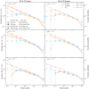 |
Fig. 16 2D accretion rate, Ṁ2D, (left verticalaxis) and probability (right vertical axis) as a function of the Stokes number in UP (dotted lines), PI-Stokes
(solid lines),and PI-Epstein cases (dashed lines). Left column: compares the results between UP and PI-Stokes cases.
Right column: compares the results between UP and PI-Epstein cases. The masses of the planet from top to bottom rows:
m = 0.003,
0.01, and 0.03, respectively. Colors indicate the Mach number of the headwind of the gas:
|


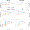 |
Fig. 17 3D accretion rate, Ṁ3D, (left vertical axis) and probability (right vertical axis) as a function of the Stokes number in UP-m001 (dotted lines), PI-Stokes-m001 (solid lines), and PI-Epstein-m001 cases (dashed lines). Left column: compares the results between UP and PI-Stokes cases. Right column: compares the results between UP and PI-Epstein cases. Colors indicate the turbulent parameter, α. The open and filled squares and circles denote the regimes of pebble accretion and the planet-induced gas flow at the given parameters. |
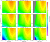 |
Fig. 18 Accretion probability as a function of the planetary mass and the Stokes number for the Mach number
|

4 Discussion
4.1 Flow transition mass
We describe the transition from the flow-shear to the flow-headwind regime in Sect. 3.3, where we derive an analytical estimation that distinguishes these hydrodynamical regimes. A planet has an isolated envelope whose size is ~ 0.5 RBondi (Kurokawa & Tanigawa 2018). The horseshoe streamlines are formed at the corotation radius for the gas. Here, we define the flow transition mass, which describes the transition from the flow-shear to flow-headwind regime. It is given by the solution of the following equation:
 (24)
(24)
The left-hand side of Eq. (24) corresponds to the maximum x-coordinates of the horseshoe region (the right edge). The right-hand side of Eq. (24) corresponds to the minimum x-coordinate of an isolated envelope (left edge). The width of the horseshoe region can be described by (Masset & Benítez-Llambay 2016):
 (25)
(25)
As discussed in Sect. 4.2.1 in Paper I, Eq. (25) agrees with the half width of the horseshoe region of our hydrodynamical simulation when m ≳ 0.1, but otherwise it is an overestimation. From our series of hydrodynamical simulations, we find that the half width of the horseshoe region for the range of planetary masses considered in this study can be described by:
 (26)
(26)
We find thatthe width of the horseshoe region decreases slightly as the Mach number increases, but it does not decrease by an order. Considering the detailed scaling with  is beyond the scope of this study. We assume that the width of the horseshoe region for the range of the planetary masses considered in this study is always given by Eq. (26). From Eqs. (24)–(26), the flow transition mass can bedescribed by
![Mathematical equation: \begin{eqnarray}m_{\textrm{t,\,flow}}= \left\{\begin{array}{@{}ll} &\displaystyle\left(-1.05\gamma^{-1/4}+\sqrt{1.1025\gamma^{-1/2}+\frac{4}{3}\mathcal{M}_{\textrm{hw}}}\,\,\right)^{2},\hspace*{1.5pc}\hfill(27) \\[6pt] &\displaystyle\hspace{120pt} (\text{for } m\gtrsim0.1),\nonumber \\[6pt] &\displaystyle\frac{4}{15}\mathcal{M}_{\textrm{hw}},\hspace{83pt} (\text{for } m\lesssim0.1),\hspace*{1.5pc}\hfill(28) \end{array}\right. \end{eqnarray}](/articles/aa/full_html/2020/11/aa39153-20/aa39153-20-eq56.png)
where we only take the positive root in Eq. (27). We plotted the larger of Eqs. (27) and (28) in Fig. 19. We note that we do not consider the reduction of the width of the horseshoe region due to the strong headwind of the gas. Thus we may underestimate the flow transition mass, particularly when  . In the MMSN model, the Mach number of the headwind has an order of ~ 0.1 even in the outer region of the disk (~100 au). Thus, Eq. (28) can be applied to a wide range of our disk model. From Eq. (28), the dimensional flow transition mass in the MMSN model can be described by
 (29)
(29)
Based on Fig. 19, we can divide our results into four categories.
When m > max(mt, peb, mt, flow), where mt, peb is the transition mass for pebble accretion (Eq. (A.4)), the accretion and flow regime are both in the shear regime (Fig. 20a). As shown in Paper I, the accretion probability of pebbles in the PI-Stokes case matches when St ≳ 3 × 10⁻³–10−2, or even smaller in the UP case when St falls below the preceding value in 2D. When m = 0.003, the influence of the planet-induced gas flow is too weak to affect pebble accretion for the range of the Stokes number considered in this study. In 3D, the accretion probability in PI-Stokes case matches or is slightly larger (smaller) than in the UP case when m ≥ 0.1 (m ≤ 0.03) for St ≲ 10−3–10−2. The width of the horseshoe region increases as the planetary mass increases. The reduction of the accretion cross-section and the increase in relative velocity cancel each other out when m ≥ 0.1. In the PI-Epstein case, since the reduction of the accretion window becomes more significant than those in the PI-Stokes case, the increase in the relative velocity does not fully offset its reduction. Therefore, the accretion probability in the PI-Epstein case tends to be smaller than in the UP case, both in 2D and in 3D.
When mt, flow < m < mt, peb, the accretion occurs in the headwind regime, but the planet-induced gas flow is in the shear regime (Fig. 20b). As in the case above, St satisfies the following relation in our parameter space: St ≲ 10−3. The pebbles tend to follow the gas streamlines. The conclusion from Paper I can be applied. The accretion window decreases in the planet-induced gas flow. The reduction of the accretion window and the increase in relative velocity due to the horseshoe flow cancel each other out.
When mt, peb < m < mt, flow, the accretion occurs in the shear regime, but the planet-induced gas flow is in the flow-headwind regime (Fig. 20c). As in the case above, St satisfies the following relation in our parameter space: St ≳ 10−3 and pebblesare less affected by the gas flow. Pebbles coming from the region where x < xpeb, cor experience fast radial drift, and do not accrete onto the planet. The accretion probability in both PI-Stokes and PI-Epstein cases match that in the UP case.
When m < min(mt, peb, mt, flow), the accretion and flow regime are both in the headwind regime (Fig. 20d). Pebbles coming from the region where x < xpeb, cor experience fast radial drift and do not accrete onto the planet. The accretion probability is larger in the PI-Stokes case than in the UP case. In the PI-Epstein case, the accretion probability is smaller than in the UP case. We find a significant enhancement of pebble accretion when m ≥ 0.01 both in 2D and in 3D. The achieved accretion probability for the pebbles with St = 10−4 in the PI-Stokes case is larger by an order of magnitude than in the UP case.
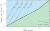 |
Fig. 19 Flow transition mass as a function of the Mach number of the headwind of the gas (black solid line). Dashed lines correspond to the pebble transition mass with different Stokes numbers (Eq. (A.4)). Blue and green regions correspond to the flow-shear and the flow-headwind regime, respectively. Since our study does not deal with gap formation (related to high-mass planets; Sect. 4.3.3), the range of the vertical axis is set to m ≤ 3. |
 |
Fig. 20 Schematic illustration of the flow structure and the trajectories of accreted pebbles at the midplane region. We classify the results obtained in both Paper I and this study into four categories based on the relation between m, mt, flow, and mt,peb. We note that the gas streamlines and the trajectories of accreted pebbles are rough outlines and may differ slightly from the actual ones. |
4.2 Comparison to previous studies
Assuming a case with 2D and inviscid fluid, Ormel (2013) derived the steady state solution of 2D flow around an embedded planet. The author calculated the trajectories of small particles using the derived flow pattern. Ormel (2013) showed the trajectories of pebbles with St = 10−4, 10−3, and 10−2 around the planet, with m = 0.01 (Fig. 12 of Ormel 2013). Two cases are shown:  and
and  . The latter case satisfies m < min(mt, peb, mt, flow) for St ≤ 10−1, where the accretion and flow regime are both in the headwind regime. Thus, the accretion of pebbles is expected to be promoted based on our results. However, accretion of small dust particles is suppressed in Ormel (2013). A plausible reason is that the size of the atmosphere is different in 2D and 3D. Ormel (2013) found that the averaged size of the atmosphere in 2D is ~ RBondi when m = 0.01 and
  . The small dust particles follow the gas streamlines outside the Bondi radius, and they passed the planet without breaking through the atmosphere. In our study, the size of an isolated envelope is ≲ 0.5RBondi (Kurokawa & Tanigawa 2018). In 3D, the small size of an isolated envelope allows pebbles to approach close to the planet. The extension of the Bondi crossing time of pebbles due to the recycling flow further promotes pebble accretion.
Rosenthal et al. (2018) introduced flow isolation mass,  , as the solution of RBondi = RHill. In our dimensionless unit, the flow isolation mass is described by
  . Based on the analytical argument without the influence of the planet-induced gas flow, these latter authors found that pebble accretion for all pebble sizes is inhibited when the planetary mass exceeds the flow isolation mass,
  . When
  , we find that m > mt, flow for a wide range of the disk where
  (Fig. 19). When the planetary mass reaches the flow isolation mass (Rosenthal et al. 2018), the planet-induced gas flow is in the flow-shear regime. In the flow-shear regime, we find that the accretion of pebbles with St ≲ 10−3 is suppressed significantly when we assumed the Epstein gas drag regime, but the accretion probability of pebbles with St ≳ 10−3 in the planet-induced gas flow is comparable to that of the unperturbed flow Paper (I). The difference is likely due to the smaller size of the bound atmosphere and complicated recycling flow patterns, both of which were not taken into account in Rosenthal et al. (2018).
Moreover, Kuwahara et al. (2019) found that the suppression of pebble accretion by the gas flow would not be expected when St ≳ 0.4, even for the higher-mass planets (m > 0.3). As the planetary mass increases, the speed of the outflow at the midplane region increases (Kuwahara et al. 2019). Our simulations are performed for the planetary mass with at most m = 0.3 (Paper I), the suppression of pebble accretion due to the gas flow might be prominent for the larger Stokes number when we assume m > 0.3. However, comparing the outflow speed to the terminal velocity of pebbles, Kuwahara et al. (2019) found that the suppression of pebble accretion due to the midplane outflow is limited to St ≲ 0.4 (see Fig. 9 of Kuwahara et al. 2019).
4.3 Implications for the growth of protoplanets
In Paper I, assuming the distribution of the turbulence strength and the size of the solid materials, we proposed a formation scenario of planetary systems to explain the distribution of exoplanets (the dominance of super-Earths at < 1 au (Fressin et al. 2013; Weiss & Marcy 2014) and a possible peak in the occurrence of gas giants at ~ 2–3 au (Johnson et al. 2010; Fernandes et al. 2019), as well as the architecture of the Solar System). We divided the disk into three sections according to previous studies and assumed turbulence strength in each section as: α ~ 10−5 (≲ 1 au), α ~ 10−3 (~ 1–10 au), and α ~ 10−4 (~ 10 au) (Malygin et al. 2017; Lyra & Umurhan 2019). Given the size distribution of the solid materials in a disk (Okuzumi & Tazaki 2019), we assumed that the pebbles have St ~ 10−3 (≲ 1 au), St ~ 3 × 10⁻² (~ 1–10 au), and St ~ 3 × 10⁻³ (~ 10 au; Fig. 21). In Paper I, we considered the growth of the protoplanet with m ~ 0.03. The accretion and flow regime were both in the shear regime. In other words, we focused on the late stage of planet formation. Here, we adopt the same assumption for the distribution of the turbulence strength and the size of the solid materials to be consistent, but we consider the growth of the protoplanets based on m ~ 0.003. Thus, we consider an earlier phase of planet formation compared to that presented in Paper I.
4.3.1 Pebble accretion in smooth disks
We first consider the growth of the protoplanets in a smooth disk. We do not consider any substructures in a disk (e.g., the gaps and rings). The Mach number in the MMSN model is given by  . The planet-induced gas flow around the planet with m = 0.003 is in the flow-headwind regime for a wide range of the disk (a ≳ 0.1 au). In contrast to Paper I, where the achieved accretion probability in the planet-induced gas flow was very low (Pacc ~ 3 × 10⁻⁴) compared to that in the unperturbed flow (Pacc ~ 7 × 10⁻²) for m = 0.03 at the inner region of thedisk (<1 au), we would expect that the accretion probability in the planet-induced gas flow would be almost identical to that in the unperturbed flow across the entire region of the disk. From Fig. 18, we can see that the planet-induced gas flow has little effect on the accretion probability for the range of the Stokes number assumed here (St ≥ 10−3). Thus, in the early phase of planet formation, the growth rate of the protoplanets can be estimated by the analytical arguments which is developed in the unperturbed flow (e.g., Ormel 2017; Liu & Ormel 2018; Ormel & Liu 2018). Only in exceptional cases, namely, where m < min(mt, peb, mt, flow),
  , and the Stokes drag law is adopted, the growth of the protoplanets would be accelerated (Fig. 18h). When the planetary mass reaches m ≳ 0.03 (Mpl ≳ 0.36 M⊕ at 1 au), the accretion of small pebbles (St ≲ 10−3) in the planet-induced gas flow begins to be suppressed in the region where
  (Figs. 18c and f).
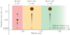 |
Fig. 21 Schematic illustration of the growth of protoplanets. The brown filled circles denote the protoplanets. The assumed Stokes numbers and the turbulence strengths are shown. The transition from the Stokes to the Epstein regime occurs at ~ 0.6 au in ourparameter set. In the early phase of planetary growth, the planet-induced gas flow does not inhibit pebble accretion for a range of the Stokes numbers considered here. When the planetary mass reaches m ~ 0.03 (the planet-induced flow isolation mass, mPI, iso), pebble accretion begins to be suppressed only in the inner region of the disk. The subsequent growth of the protoplanets in the inner region of the disk is highly suppressed (dashed arrow; Paper I) |
4.3.2 Pebble accretion at the pressure bump
Recent observations have shown the gas and ring structures in a disk (e.g., ALMA Partnership 2015; Pinte et al. 2015; Andrews et al. 2016, 2018; Isella et al. 2016; Cieza et al. 2017; Fedele et al. 2018; Long et al. 2018, 2020; Dullemond et al. 2018; van der Marel et al. 2019). Several mechanisms have been proposed to explain the ring structure in a disk: the dust accumulation at the edge of the dead-zone (Flock et al. 2015), dust growth at snow lines (Zhang et al. 2015; Okuzumi et al. 2016), secular gravitational instability (Takahashi & Inutsuka 2014, 2016; Tominaga et al. 2018, 2019), or gap opening due to the presence of planets (Kanagawa et al. 2015, 2016; Dong et al. 2015; Dipierro et al. 2015). The possible origin of the ring is still being debated. When the ring structure is related to the dust getting trapped in radial pressure bumps (Dullemond et al. 2018), where  , the contribution of the headwind of the gas vanishes. Even in the outer region of the disk, the accretion and flow regime are both in the shear regime at the pressure bump.
Figures 18b and c show the accretion probability for  , but corresponding to the case where the accretion and flow regime are both in the shear regime. Thus, we can estimate the accretion probability for the planet with m = 0.003 at the pressure bump from Figs. 18b and c. From Figs. 18b and c, the accretion probability in the planet-induced gas flow for the planet with m = 0.003 is identical to that in the unperturbed flow for a range of the Stokes number considered here, St ≥ 10−3. Same as in the smooth disks, in the early phase of planet formation, the growth rate of the protoplanets can be estimated by the analytical arguments which is developed in the unperturbed flow (e.g., Ormel 2017; Liu & Ormel 2018; Ormel & Liu 2018). At the pressure bump, the enhancement of pebble accretion due to the planet-induced gas flow would never occur. Nevertheless, an increase in the dust-to-gas ratio at the pressure bump would lead to an increase in the accretion rate of pebbles. When the planetary mass reaches m ≳ 0.03 (Mpl ≳ 0.36 M⊕ at 1 au), the suppression of pebble accretion for St ≲ 10−3 in the planet-induced gas flow becomes prominent (Figs. 18b and c, see also Figs. 10 and 11 in Paper I).
4.3.3 Pebble accretion for high-mass planets
Our study is focused on low-mass planets (Fig. 1). High-mass planets shape global pressure gradient, and an induced pressure maximum inhibits pebble accretion (Lambrechts et al. 2014; Bitsch et al. 2018). Planets with m > 3 form a gap in a disk (Lin & Papaloizou 1993). Pebble isolation initiates at a lower planetary mass in a disk with smaller turbulent viscosity (Bitsch et al. 2018). Fung & Lee (2018) reported that a planet with m ≃ 0.4 (6.6 M⊕ at ~ 1.5 au) can form a pressure bump in an inviscid disk.
4.3.4 Planet-induced flow isolation mass
The dimensionless planetary masses of 0.03 can be regarded as a type of isolation mass, particularly when St ≲ 10−3 and  . In this specific case, pebble accretion would be expected to halt before the mass of the protoplanets reaches a pebble isolation mass (Lambrechts et al. 2014):
 (30)
(30)
A subsequent study derived a detailed pebble isolation mass (Bitsch et al. 2018):
![Mathematical equation: \begin{align*} M_{\textrm{iso}}\simeq25\left(\frac{H/r}{0.05}\right)^3\left[0.34\left(\frac{3}{\log\alpha}\right)^4+0.66\right]\,M_{\oplus}.\end{align*}](/articles/aa/full_html/2020/11/aa39153-20/aa39153-20-eq74.png) (31)
(31)
Equation (31) gives
 (32)
(32)
when we assume  and α = 10−3. In our dimensionless unit, Eq. (32) can be described by
 (33)
(33)
When we refer m = 0.03 as planet-induced flow isolation mass, mPI, iso, and then we have
 (34)
(34)
4.4 Implications for the origins of the architecture of a planetary system
In Paper I,when tracking the growth of the planet with m = 0.03, we introduced a formation scenario of planetary systems, where pebble accretion is suppressed only in the inner region of the disk (≲ 1 au). As discussed in Sects. 4.3.1 and 4.3.2, the planet-induced gas flow does not affect the accretion probability of pebbles in the earlier phase of planet formation as compared to the situation considered in Paper I (Fig. 21).
When we focus on the region where <100 au ( ), and the planetary mass exceeds m > 0.03, the planet-induced gas flow is always in the flow-shear regime (Fig. 19). Based on the discussion in Paper I, we once again propose a possible scenario for the distribution of the exoplanets.
In the first instance, rocky terrestrial planets or super-Earths are formed in the inner region of the disk, ≲ 1 au, where α and St are small. The protoplanets accrete pebbles without the influence of planet-induced gas flow and reach planet-induced flow isolation mass, mPI, iso (~ 0.36 M⊕ at 1 au). When the mass of the protoplanetsreaches m ≳ mPI, iso, the suppression of pebble accretion due to the planet-induced gas flow is prominent (Paper I). The subsequent growth of the protoplanets is highly suppressed. Within the growth track, the small rocky terrestrial planets may experience inward migration. Within ≲ 0.6 au, the gas draglaw switches to the Stokes regime in our parameter set. This leads to an increase in the accretion probability of pebbles (Paper I). The small rocky protoplanets may also experience giant impacts. These events lead to the formation of super-Earths.
In the next instance, gas giants are formed in the middle region of the disk, ~ 1–10 au, where α and St are larger than those in the inner region. Since the Stokes number is large, the planet-induced gas flow does not inhibit the growth of the protoplanets even though the mass of the protoplanets reaches m ≳ mPI, iso (Paper I). Thus, we expect that the planets might exceed the critical core mass within the typical lifetime of the disk. The final mass of the protoplanets is set by the pebble isolation due to formation of pressure bump (Lambrechts et al. 2014; Bitsch et al. 2018).
In the last instance, ice giants are formed in the outer region, where α and St are smaller than those in the middle region. In the same way as in the middle region, planet-induced gas flow does not inhibit the growth of the protoplanets until their mass reaches m ~ mPI, iso. When m ≳ mPI, iso, the accretion probability in the planet-induced gas flow is reduced by a factor compared to that in the unperturbed flow (Paper I). With the accretion of a moderate amount of icy pebbles, the planets would eventually become ice giants without evolving into gas giants.
Our scenario may be helpful in explaining the distribution of exoplanets (the dominance of super-Earths at < 1 au Fressin et al. 2013; Weiss & Marcy 2014 and a possible peak in the occurrence of gas giants at ~ 2–3 au Johnson et al. 2010; Fernandes et al. 2019), as well as the architecture of the Solar System: rocky planets in the inner regions, gas giants in the middle, and icy giants in the outer regions.
The reduction of the pebble isolation mass in the inner region of the inviscid disk may cause the dichotomy that is apparent between the inner super-Earths and outer gas giants (Fung & Lee 2018). However, the small pebbles (St ≲ 10−3) may not be trapped at the local pressure maxima and, thus, they continue to contribute to the growth of the planet (Bitsch et al. 2018). The planet-induced flow isolation has the potential to explain the dichotomy even if the inward drift of small pebbles does not stop at the pressure maxima.
5 Conclusions
Following Paper I, in this work, we investigate the influence of 3D planet-induced gas flow on pebble accretion. We considered nonisothermal, inviscid gas flow and performed a series of 3D hydrodynamical simulations on a spherical polar grid that has a planet placed at its center. We then numerically integrated the equation of the motion of pebbles in 3D using hydrodynamical simulation data. We conducted three types of orbital calculations for pebbles in this study: in the unperturbed flow (UP case); in the planet-induced gas flow in the Stokes regime (PI-Stokes case); and in the planet-induced gas flow in the Epstein regime (PI-Epstein case). The subject of the range of dimensionless planetary mass in this study is m = 0.003–0.03, which corresponds to a size ranging from three Moon masses to three Mars masses, Mpl = 0.036–0.36 M⊕, orbiting a solar-mass star at 1 au. Following Paper I, where only the shear regime of pebble accretion was considered, we extend our study tothe headwind regime of pebble accretion in this study. Paper II focuses on the headwind regime of pebble accretion. We summarize our main findings as follows.
- 1.
The planet-induced gas flow can be divided into two regimes: the flow-shear and flow-headwind regimes. In theflow-shear regime, the planet-induced gas flow has a vertically rotational symmetric structure (Ormel et al. 2015; Fung et al. 2015, 2019; Lambrechts & Lega 2017; Cimerman et al. 2017; Kurokawa & Tanigawa 2018; Kuwahara et al. 2019; Béthune & Rafikov 2019). Gas from the disk enters the gravitational sphere at high latitudes and exits through the midplane region of the disk. The horseshoe flow lies across the orbit of the planet and has a columnar structure in the vertical direction. In the flow-headwind regime, the headwind of the gas breaks the symmetric structure (Ormel et al. 2015; Kurokawa & Tanigawa 2018). The planetary envelope is exposed to the headwind of the gas. Gas from the disk enters the gravitational sphere at low latitudes and exits at high latitudes of the gravitational sphere. The horseshoe flow lies inside the planetary orbit. We derived the flow transition mass analytically, mt, flow, which discriminates between the flow-headwind and flow-shear regimes.
- 2.
In the flow-headwind regime, the trajectories of pebbles with St ≲ 10−3 in the planet-induced gas flow differ significantly from those in the unperturbed flow. The outflow in the fourth quadrant of the x-y plane deflects the trajectories of pebbles. The pebbles are jammed outside the planetary orbit. The horseshoe flow shifts significantly to the negative direction in the x-axis. Because of the absence of the horseshoe flow and the outflow in the anterior region of the planetary orbit, pebbles passing near the planetary orbit are susceptible to becoming entangled in the recycling flow in the flow-headwind regime. When pebbles enter the Bondi sphere and get entangled in the recycling flow, the relative velocity of pebbles is reduced by an order of magnitude because of the low speed of gas flow. This leads to an increase in the Bondi crossing time of pebbles. Thus, pebble accretion is enhanced in the planet-induced gas flow when pebbles are well-coupled to the gas.
- 3.
From the relation between m, mt, flow and mt, peb, we classify the results obtained in both Paper I and this study into four categories. When m > max(mt, peb, mt, flow) and mt, flow < m < mt, peb, we find that the outcome is identical to that in Paper I. When mt, peb < m < mt, flow, the influence of the planet-induced gas flow cannot be seen. In particular, when m < min(mt, peb, mt, flow) and the Stokes gas drag law is adopted, pebble accretion is enhanced due to the planet-induced gas flow. The width of the accretion window, accretion cross-section, and the accretion probability of pebbles in the planet-induced gas flow are larger than those in the unperturbed flow.
Following Paper I, we assumed that the global structure of the disk in terms of the distribution of the turbulence parameter and the size distribution of the solid materials in a disk based on previous studies (Malygin et al. 2017; Lyra & Umurhan 2019; Okuzumi & Tazaki 2019). In Paper II, we consider an earlier phase of planet formation (m ≲ 0.03) compared to the what we considered in Paper I. We find that the planet-induced gas flow has little effect on pebble accretion for a range of the Stokes number assumed here, namely, St ≥ 10−3. Based on the discussion in Paper I, we conclude that the suppression of pebble accretion due to the planet-induced gas flow works in the late stage of planet formation (m ≳ 0.03), in particular, in the inner region of the disk (≲1 au). We find that the dimensionless planetary masses of 0.03 can be regarded as the planet-induced flow isolation mass, mPI, iso, in a specific case where St ≲ 10−3 and  . This may be helpful in explaining the distribution of exoplanets with regard to the dominance of super-Earths at < 1 au (Fressin et al. 2013; Weiss & Marcy 2014) and a possible peak in the occurrence of gas giants at ~ 2–3 au (Johnson et al. 2010; Fernandes et al. 2019), as well as the architecture of the Solar System, both of which exhibit small inner and large outer planets.
Acknowledgements
We would like to thank the anonymous referee for their constructive comments. We thank Athena++ developers: James M. Stone, Kengo Tomida, and Christopher White. Numerical computations were in part carried out on Cray XC50 at theCenter for Computational Astrophysics at the National Astronomical Observatory of Japan. A.K. was supported by JSPS KAKENHI Grant number 20J20681. H.K. was supported by JSPS KAKENHI Grant number 17H06457, 18K13602, 19H05072, and 19H01960.
Appendix A Analytical estimation of pebble accretion
In the settling regime, the maximum impact parameter of accreted pebbles in the unperturbed flow is expressed by:
![Mathematical equation: \begin{align*}b_{x}\simeq \left\{\!\!\!\begin{array}{l}b_{x,\textrm{hw}}=\displaystyle2\!\sqrt{\frac{m\textrm{St}}{\mathcal{M}_{\textrm{hw}}}}, \ (m\!<\! m_{\textrm{t,\,peb}}: \textrm{headwind regime}),\\[7pt] b_{x,\textrm{sh}}=\displaystyle2\,\textrm{St}^{1/3}\ R_{\textrm{Hill}}, \ (m\!>\! m_{\textrm{t,\,peb}}: \textrm{shear regime}),\end{array}\right. \end{align*}](/articles/aa/full_html/2020/11/aa39153-20/aa39153-20-eq81.png)
(Ormel & Klahr 2010; Lambrechts & Johansen 2012; Guillot et al. 2014; Ida et al. 2016; Sato et al. 2016), where mt, peb is the transition mass for pebble accretion:
 (A.3)
(A.3)
(Lambrechts & Johansen 2012; Johansen & Lambrechts 2017; Ormel 2017). The dimensional pebble-transition mass in the MMSN model can be described by:
 (A.4)
(A.4)
In the current study, we refer to the transition mass which divide the accretion regime of pebbles as “pebble transition mass” to distinguish pebble-transition mass from flow-transition mass, which determines the regime of the planet-induced gas flow (Eqs. (27) and (28)).
Appendix B Additional figures
 |
Fig. B.1 Same as Fig. 17, but with results obtained from UP-m0003 case (dotted lines), PI-Stokes-m0003 case (solid lines), and PI-Epstein-m0003 case (dashed lines). |
 |
Fig. B.2 Same as Fig. 17, but with results obtained from UP-m003 case (dotted lines), PI-Stokes-m003 case (solid lines), and PI-Epstein-m003 case (dashed lines). |
References
- ALMA Partnership (Brogan, C. L., et al.) 2015, ApJ, 808, L3 [NASA ADS] [CrossRef] [Google Scholar]
- Andrews, S. M., Wilner, D. J., Zhu, Z., et al. 2016, ApJ, 820, L40 [NASA ADS] [CrossRef] [Google Scholar]
- Andrews, S. M., Huang, J., Pérez, L. M., et al. 2018, ApJ, 869, L41 [NASA ADS] [CrossRef] [Google Scholar]
- Béthune, W., & Rafikov, R. R. 2019, MNRAS, 488, 2365 [NASA ADS] [CrossRef] [Google Scholar]
- Bitsch, B., Morbidelli, A., Johansen, A., et al. 2018, A&A, 612, A30 [NASA ADS] [CrossRef] [EDP Sciences] [Google Scholar]
- Chapman, S., & Cowling, T. G. 1970, The Mathematical Theory of Non-uniform Gases. An Account of the Kinetic Theory of Viscosity, Thermal Conduction and Diffusion in Gases (Cambridge: Cambridge University Press) [Google Scholar]
- Cieza, L. A., Casassus, S., Pérez, S., et al. 2017, ApJ, 851, L23 [NASA ADS] [CrossRef] [Google Scholar]
- Cimerman, N. P., Kuiper, R., & Ormel, C. W. 2017, MNRAS, 471, 4662 [NASA ADS] [CrossRef] [Google Scholar]
- Cuzzi, J. N., Dobrovolskis, A. R., & Champney, J. M. 1993, Icarus, 106, 102 [NASA ADS] [CrossRef] [Google Scholar]
- Dipierro, G., Price, D., Laibe, G., et al. 2015, MNRAS, 453, L73 [NASA ADS] [CrossRef] [Google Scholar]
- Dong, R., Zhu, Z., & Whitney, B. 2015, ApJ, 809, 93 [NASA ADS] [CrossRef] [Google Scholar]
- Dubrulle, B., Morfill, G., & Sterzik, M. 1995, Icarus, 114, 237 [NASA ADS] [CrossRef] [Google Scholar]
- Dullemond, C. P., Birnstiel, T., Huang, J., et al. 2018, ApJ, 869, L46 [NASA ADS] [CrossRef] [EDP Sciences] [Google Scholar]
- Fedele, D., Tazzari, M., Booth, R., et al. 2018, A&A, 610, A24 [NASA ADS] [CrossRef] [EDP Sciences] [Google Scholar]
- Fernandes, R. B., Mulders, G. D., Pascucci, I., Mordasini, C., & Emsenhuber, A. 2019, ApJ, 874, 81 [NASA ADS] [CrossRef] [Google Scholar]
- Flock, M., Ruge, J., Dzyurkevich, N., et al. 2015, A&A, 574, A68 [NASA ADS] [CrossRef] [EDP Sciences] [Google Scholar]
- Fressin, F., Torres, G., Charbonneau, D., et al. 2013, ApJ, 766, 81 [NASA ADS] [CrossRef] [Google Scholar]
- Fung, J., & Lee, E. J. 2018, ApJ, 859, 126 [NASA ADS] [CrossRef] [Google Scholar]
- Fung, J., Artymowicz, P., & Wu, Y. 2015, ApJ, 811, 101 [NASA ADS] [CrossRef] [Google Scholar]
- Fung, J., Zhu, Z., & Chiang, E. 2019, ApJ, 887, 152 [CrossRef] [Google Scholar]
- Guillot, T., Ida, S., & Ormel, C. W. 2014, A&A, 572, A72 [NASA ADS] [CrossRef] [EDP Sciences] [Google Scholar]
- Hayashi, C., Nakazawa, K., & Nakagawa, Y. 1985, in Protostars and Planets II, eds. D. C. Black, & M. S. Matthews (Tucson, AZ: University of Arizona Press), 1100 [Google Scholar]
- Ida, S., & Nakazawa, K. 1989, A&A, 224, 303 [NASA ADS] [Google Scholar]
- Ida, S., Guillot, T., & Morbidelli, A. 2016, A&A, 591, A72 [NASA ADS] [CrossRef] [EDP Sciences] [Google Scholar]
- Isella, A., Guidi, G., Testi, L., et al. 2016, Phys. Rev. Lett., 117, 251101 [NASA ADS] [CrossRef] [Google Scholar]
- Johansen, A., & Lambrechts, M. 2017, Ann. Rev. Earth Planet. Sci., 45, 359 [NASA ADS] [CrossRef] [Google Scholar]
- Johnson, J. A., Aller, K. M., Howard, A. W., & Crepp, J. R. 2010, PASP, 122, 905 [NASA ADS] [CrossRef] [Google Scholar]
- Kanagawa, K. D., Muto, T., Tanaka, H., et al. 2015, ApJ, 806, L15 [NASA ADS] [CrossRef] [Google Scholar]
- Kanagawa, K. D., Muto, T., Tanaka, H., et al. 2016, PASJ, 68, 43 [NASA ADS] [Google Scholar]
- Kurokawa, H.,& Tanigawa, T. 2018, MNRAS, 479, 635 [NASA ADS] [CrossRef] [Google Scholar]
- Kuwahara, A.,& Kurokawa, H. 2020, A&A, 633, A81 [NASA ADS] [CrossRef] [EDP Sciences] [Google Scholar]
- Kuwahara, A., Kurokawa, H., & Ida, S. 2019, A&A, 623, A179 [NASA ADS] [CrossRef] [EDP Sciences] [Google Scholar]
- Lambrechts, M., & Johansen, A. 2012, A&A, 544, A32 [Google Scholar]
- Lambrechts, M., & Lega, E. 2017, A&A, 606, A146 [NASA ADS] [CrossRef] [EDP Sciences] [Google Scholar]
- Lambrechts, M., Johansen, A., & Morbidelli, A. 2014, A&A, 572, A35 [NASA ADS] [CrossRef] [EDP Sciences] [Google Scholar]
- Lambrechts, M., Morbidelli, A., Jacobson, S. A., et al. 2019, A&A, 627, A83 [NASA ADS] [CrossRef] [EDP Sciences] [Google Scholar]
- Lin, D. N. C., & Papaloizou, J. C. B. 1993, in Protostars and Planets III, eds. E. H. Levy, & J. I. Lunine (Tucson, AZ: University of Arizona Press), 749 [Google Scholar]
- Liu, B., & Ormel, C. W. 2018, A&A, 615, A138 [NASA ADS] [CrossRef] [EDP Sciences] [Google Scholar]
- Long, F., Pinilla, P., Herczeg, G. J., et al. 2018, ApJ, 869, 17 [NASA ADS] [CrossRef] [Google Scholar]
- Long, F., Pinilla, P., Herczeg, G. J., et al. 2020, ApJ, 898, 36 [CrossRef] [Google Scholar]
- Lyra, W., & Umurhan, O. M. 2019, PASP, 131, 072001 [NASA ADS] [CrossRef] [Google Scholar]
- Malygin, M. G., Klahr, H., Semenov, D., Henning, T., & Dullemond, C. P. 2017, A&A, 605, A30 [NASA ADS] [CrossRef] [EDP Sciences] [Google Scholar]
- Masset, F. S., & Benítez-Llambay, P. 2016, ApJ, 817, 19 [NASA ADS] [CrossRef] [Google Scholar]
- Nakagawa, Y., Sekiya, M., & Hayashi, C. 1986, Icarus, 67, 375 [NASA ADS] [CrossRef] [Google Scholar]
- Okuzumi, S., & Tazaki, R. 2019, ApJ, 878, 132 [NASA ADS] [CrossRef] [Google Scholar]
- Okuzumi, S., Momose, M., Sirono, S.-i., Kobayashi, H., & Tanaka, H. 2016, ApJ, 821, 82 [NASA ADS] [CrossRef] [Google Scholar]
- Ormel, C. W. 2013, MNRAS, 428, 3526 [NASA ADS] [CrossRef] [Google Scholar]
- Ormel, C. W. 2017, Astrophys. Space Sci. Lib., 445, 197 [NASA ADS] [CrossRef] [Google Scholar]
- Ormel, C. W., & Klahr, H. H. 2010, A&A, 520, A43 [NASA ADS] [CrossRef] [EDP Sciences] [Google Scholar]
- Ormel, C. W., & Liu, B. 2018, A&A, 615, A178 [NASA ADS] [CrossRef] [EDP Sciences] [Google Scholar]
- Ormel, C. W., Shi, J.-M., & Kuiper, R. 2015, MNRAS, 447, 3512 [NASA ADS] [CrossRef] [Google Scholar]
- Pinte, C., Dent, W. R., Ménard, F., et al. 2015, ApJ, 816, 25 [Google Scholar]
- Popovas, A., Nordlund, Å., Ramsey, J. P., & Ormel, C. W. 2018, MNRAS, 479, 5136 [NASA ADS] [CrossRef] [Google Scholar]
- Popovas, A., Nordlund, Å., & Ramsey, J. P. 2019, MNRAS, 482, L107 [NASA ADS] [CrossRef] [Google Scholar]
- Rosenthal, M. M., Murray-Clay, R. A., Perets, H. B., & Wolansky, N. 2018, ApJ, 861, 74 [NASA ADS] [CrossRef] [Google Scholar]
- Sato, T., Okuzumi, S., & Ida, S. 2016, A&A, 589, A15 [NASA ADS] [CrossRef] [EDP Sciences] [Google Scholar]
- Shakura, N. I., & Sunyaev, R. A. 1973, A&A, 24, 337 [NASA ADS] [Google Scholar]
- Stone, J. M., Tomida, K., White, C. J., & Felker, K. G. 2020, ApJS, 249, 40 [CrossRef] [Google Scholar]
- Takahashi, S. Z., & Inutsuka, S.-i. 2014, ApJ, 794, 55 [NASA ADS] [CrossRef] [Google Scholar]
- Takahashi, S. Z., & Inutsuka, S.-i. 2016, AJ, 152, 184 [NASA ADS] [CrossRef] [Google Scholar]
- Tominaga, R. T., Inutsuka, S.-i., & Takahashi, S. Z. 2018, PASJ, 70, 3 [Google Scholar]
- Tominaga, R. T., Takahashi, S. Z., & Inutsuka, S. 2019, ApJ, 881, 53 [NASA ADS] [CrossRef] [Google Scholar]
- van der Marel, N., Dong, R., di Francesco, J., Williams, J. P., & Tobin, J. 2019, ApJ, 872, 112 [NASA ADS] [CrossRef] [Google Scholar]
- Weidenschilling, S. J. 1977a, Astrophys. Space Sci., 51, 153 [NASA ADS] [CrossRef] [Google Scholar]
- Weidenschilling, S. J. 1977b, MNRAS, 180, 57 [Google Scholar]
- Weiss, L. M., & Marcy, G. W. 2014, ApJ, 783, L6 [NASA ADS] [CrossRef] [Google Scholar]
- White, C. J., Stone, J. M., & Gammie, C. F. 2016, ApJS, 225, 22 [NASA ADS] [CrossRef] [Google Scholar]
- Youdin, A. N., & Lithwick, Y. 2007, Icarus, 192, 588 [NASA ADS] [CrossRef] [Google Scholar]
- Zhang, K., Blake, G. A., & Bergin, E. A. 2015, ApJ, 806, L7 [NASA ADS] [CrossRef] [Google Scholar]
In this study, we use “headwind” and “shear” regimes as names to distinguish the pebble accretion regimes used in Ormel (2017). These regimes are referred to as “Bondi” and “Hill” regimes in Lambrechts & Johansen (2012).
In Paper I, we assume a = 0.1 au in Eq. (2). However, the size of the Bondi radius is larger than the size of the physical radius of the planet when m ≲ 0.005 at a = 0.1 au. This means that the planet does not have an envelope. To ensure that even low-mass planets (m ≲ 0.005) has an atmosphere, we assume a = 1 au in this study. It ensures that RBondi > Rpl for all of the parameter sets considered in our hydrodynamical simulations.
In Paper I, the unperturbed flow case is referred to as the “Shear case”.
For simplicity, we do not consider the switch from the Epstein to the Stokes regime in the vicinity of the planet in both Paper I and this study. The mean free path of the gas becomes smaller as the gas density increases and may lead to a switch of the drag law in the region very close to the planet.
In contrast, when the planetary mass is large, m ≳ 0.1, the reduction of the accretion cross-section and the increase in relative velocity cancel each other out. Consequently, the accretion probability becomes comparable to that of the unperturbed flow (see Sect. 3.4.2 of Paper I).
All Tables
All Figures
|
Fig. 1 Summary of parameter surveys in Paper I and II. The parameter spaces investigated in both Paper I and II are shown in redand yellow filled squares, respectively. The vertical and horizontal axes are the dimensionless planetary mass, m (Eq. (1)), and the Mach number of the headwind of the gas,
|
| In the text | |
|
Fig. 2 Schematic picture of an orbital calculation of pebbles. A planet is located at the origin of the co-rotational frame. The dashed line represents the outer boundary of the hydrodynamical simulations. The starting point of orbital calculation is beyond the outer boundary of hydrodynamical simulations. Its y-component is fixed at 40 RHill (Ida & Nakazawa 1989). The x- and z-coordinates of the starting point of pebbles, xs and zs, are the parameters. The gas velocity is assumed to be the speed of the sub-Keplerian shear both inside and outside of rout in the shear flow case of the unperturbed flow (UP-mXX-hwYY case), but is switchedto the gas velocity obtained from the hydrodynamical simulations within rout in the planet-induced flow case in the Epstein regime (PI-Epstein-mXX-hwYY case), and in the Stokes regime (PI-Stokes-mXX-hwYY case). |
| In the text | |
|
Fig. 3 Streamlines of 3D planet-induced gas flow around the planet. The result obtained from m003-hw01 at t = 50. The red, green, and blue solid lines are the recycling streamlines, the horseshoe streamlines, and the Keplerian shear streamlines, respectively. For the recycling streamlines, we only plot the streamlines which pass over the surface of the Bondi sphere. The arrows represent the direction of the gas flow. |
| In the text | |
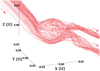 |
Fig. 4 Enlarged view of Fig. 3. We only plot the recycling streamlines. |
| In the text | |
|
Fig. 5 Flow structure around a planet with m = 0.03 at the midplane of the disk. Panel a: result obtained from m003-hw001 at t = 50. Panel b: result obtained from m003-hw003 at t = 50. Panel c: result obtained from m003-hw01 at t = 50. Color contour represents the flow speed in the y-direction. The verticaland horizontal axis are normalized by the scale height of the disk. The solid lines correspond to the specific streamlines.The dotted and dashed lines are the Bondi and Hill radius of the planet, respectively. We note that the length of the arrows does not scale with the flow speed. |
| In the text | |
|
Fig. 6 Enlarged view of Fig. 5c, but the color contour represents the flow speed in the azimuthal direction. |
| In the text | |
|
Fig. 7 Trajectories of pebbles in UP-m001-hw01 case (top) and PI-Stokes-m001-hw01 case (bottom) with different Stokes numbers at the midplane of the disk. We set zs = 0 for all cases. The red and blue solid lines correspond to the trajectories of pebbles which accreted and did not accrete onto the planet, respectively. The dashed circles show the Hill radius of the planet. The sizes of the Hill and Bondi radii are 0.15 [H] and 0.01 [H]. The black dot at the center of each panel denotes the position of the planet. The interval of pebbles at their initial locations is 0.05 [H]. The regimes of pebble accretion and the planet-induced gas flow are determined by Eqs. (A.4) and (28). |
| In the text | |
|
Fig. 8 Trajectories of pebbles in UP-m003-hw01 case (left panel) and PI-Stokes-m003-hw01 case (right panel) with St = 10−4 at the midplane of the disk. We set zs = 0. The red and blue solid lines correspond to the trajectories of pebbles which accreted and did not accrete onto the planet, respectively. The dotted-dashed and dashed circles show the Bondi and the Hill radius of the planet, respectively. The sizes of the Bondi radius and the Hill radius are 0.03 [H] and 0.22 [H]. The black dots at the center of each panel denote the position of the planet. The interval of pebbles at their initial locations is 0.003 [H]. |
| In the text | |
|
Fig. 9 Trajectories of pebbles with St = 10−4 in UP-m003-hw01 case (top) and PI-Stokes-m003-hw01 case (bottom). The height of the initial position of the pebbles is zs = 0.03 [H]. The red and blue solid lines correspond to the trajectories of pebbles which accreted and did not accrete onto the planet, respectively. The black dots at the center of each panel denote the position of the planet. The sphere around the planet represents the Bondi radius of the planet. We only plot the trajectories within the region where r < 2RHill. The interval of pebbles at their initial locations is 0.01 [H]. |
| In the text | |
|
Fig. 10 Trajectories (left) and the relative velocity of pebbles to the planet (right) with St = 10−4. Panel a: results obtained from UP-m003- hw01 case. Panel b: results obtained from PI-Stokes-m003-hw01 case. We set zs = 0 [H]. Different colors correspond to different xs as indicated in figure legends. The dots on the solid lines mark intervals of Ω−1. The black dot and the dotted-dashed circle in the left column show the position of the planet and the Bondi radius of the planet. The vertical solid and dashed lines in the right column show the size of the Bondi radius and the terminal velocity of pebbles (Eq. (23)). |
| In the text | |
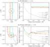 |
Fig. 11 Same as Fig. 10, but we set zs = 0.03 [H]. |
| In the text | |
|
Fig. 12 Width of the accretion window in the midplane, wacc(0), as a function of the Stokes number in the UP (dotted lines), PI-Stokes (solid lines), and the PI-Epstein cases (dashed lines). Left column: compares the results between UP and PI-Stokes cases. Right column: compares the results between UP and PI-Epstein cases. The masses of the planet from top to bottom rows: m = 0.003, 0.01, and 0.03, respectively. Colors indicate the Mach number of the headwind of the gas:
|
| In the text | |
|
Fig. 13 Accretion window with the different Stokes numbers in the UP-m001-hw003 (top) and the PI-Stokes-m001-hw003 cases (bottom). We assume α = 10−3 and the dust-to-gas ratio equal to 10−2. Color represents the density of the pebbles expressed by Eq. (18) normalized by the gas density. The vertical dashed lines correspond to the corotation radius for pebbles (Eq. (10)). The two panels in panelsa and e show the enlarged outlines of accretion windows. We note that the color contour is saturated for ρp ≲ 10−3. |
| In the text | |
|
Fig. 14 Same as Fig. 13, but in the UP-m001-hw01 case (top) and the PI-Stokes-m001-hw01 case (bottom). |
| In the text | |
|
Fig. 15 Accretion cross-section, Aacc, as a function of the Stokes number in UP (dotted lines), PI-Stokes (solid lines), and PI-Epstein cases (dashed lines). Left column: compares the results between UP and PI-Stokes cases. Right column: compares the results between UP and PI-Epstein cases. The masses of the planet from top to bottom rows: m = 0.003, 0.01, and 0.03, respectively. Colors indicate the Mach number of the headwind of the gas:
|
| In the text | |
|
Fig. 16 2D accretion rate, Ṁ2D, (left verticalaxis) and probability (right vertical axis) as a function of the Stokes number in UP (dotted lines), PI-Stokes
(solid lines),and PI-Epstein cases (dashed lines). Left column: compares the results between UP and PI-Stokes cases.
Right column: compares the results between UP and PI-Epstein cases. The masses of the planet from top to bottom rows:
m = 0.003,
0.01, and 0.03, respectively. Colors indicate the Mach number of the headwind of the gas:
|
| In the text | |
|
Fig. 17 3D accretion rate, Ṁ3D, (left vertical axis) and probability (right vertical axis) as a function of the Stokes number in UP-m001 (dotted lines), PI-Stokes-m001 (solid lines), and PI-Epstein-m001 cases (dashed lines). Left column: compares the results between UP and PI-Stokes cases. Right column: compares the results between UP and PI-Epstein cases. Colors indicate the turbulent parameter, α. The open and filled squares and circles denote the regimes of pebble accretion and the planet-induced gas flow at the given parameters. |
| In the text | |
|
Fig. 18 Accretion probability as a function of the planetary mass and the Stokes number for the Mach number
|
| In the text | |
|
Fig. 19 Flow transition mass as a function of the Mach number of the headwind of the gas (black solid line). Dashed lines correspond to the pebble transition mass with different Stokes numbers (Eq. (A.4)). Blue and green regions correspond to the flow-shear and the flow-headwind regime, respectively. Since our study does not deal with gap formation (related to high-mass planets; Sect. 4.3.3), the range of the vertical axis is set to m ≤ 3. |
| In the text | |
|
Fig. 20 Schematic illustration of the flow structure and the trajectories of accreted pebbles at the midplane region. We classify the results obtained in both Paper I and this study into four categories based on the relation between m, mt, flow, and mt,peb. We note that the gas streamlines and the trajectories of accreted pebbles are rough outlines and may differ slightly from the actual ones. |
| In the text | |
|
Fig. 21 Schematic illustration of the growth of protoplanets. The brown filled circles denote the protoplanets. The assumed Stokes numbers and the turbulence strengths are shown. The transition from the Stokes to the Epstein regime occurs at ~ 0.6 au in ourparameter set. In the early phase of planetary growth, the planet-induced gas flow does not inhibit pebble accretion for a range of the Stokes numbers considered here. When the planetary mass reaches m ~ 0.03 (the planet-induced flow isolation mass, mPI, iso), pebble accretion begins to be suppressed only in the inner region of the disk. The subsequent growth of the protoplanets in the inner region of the disk is highly suppressed (dashed arrow; Paper I) |
| In the text | |
|
Fig. B.1 Same as Fig. 17, but with results obtained from UP-m0003 case (dotted lines), PI-Stokes-m0003 case (solid lines), and PI-Epstein-m0003 case (dashed lines). |
| In the text | |
|
Fig. B.2 Same as Fig. 17, but with results obtained from UP-m003 case (dotted lines), PI-Stokes-m003 case (solid lines), and PI-Epstein-m003 case (dashed lines). |
| In the text | |
Current usage metrics show cumulative count of Article Views (full-text article views including HTML views, PDF and ePub downloads, according to the available data) and Abstracts Views on Vision4Press platform.
Data correspond to usage on the plateform after 2015. The current usage metrics is available 48-96 hours after online publication and is updated daily on week days.
Initial download of the metrics may take a while.