| Issue |
A&A
Volume 643, November 2020
|
|
|---|---|---|
| Article Number | A169 | |
| Number of page(s) | 18 | |
| Section | Numerical methods and codes | |
| DOI | https://doi.org/10.1051/0004-6361/202038726 | |
| Published online | 20 November 2020 | |
More planetary candidates from K2 Campaign 5 using TRAN_K2⋆
Konkoly Observatory, Konkoly Thege ut. 15-17, Budapest 1121, Hungary
e-mail: kovacs@konkoly.hu
Received:
23
June
2020
Accepted:
3
September
2020
Context. The exquisite precision of space-based photometric surveys and the unavoidable presence of instrumental systematics and intrinsic stellar variability call for the development of sophisticated methods that distinguish these signal components from those caused by planetary transits.
Aims. Here, we introduce the standalone Fortran code TRAN_K2 to search for planetary transits under the colored noise of stellar variability and instrumental effects. We use this code to perform a survey to uncover new candidates.
Methods. Stellar variability is represented by a Fourier series and, when necessary, by an autoregressive model aimed at avoiding excessive Gibbs overshoots at the edges. For the treatment of systematics, a cotrending and an external parameter decorrelation were employed by using cotrending stars with low stellar variability as well as the chip position and the background flux level at the target. The filtering was done within the framework of the standard weighted least squares, where the weights are determined iteratively, to allow a robust fit and to separate the transit signal from stellar variability and systematics. Once the periods of the transit components are determined from the filtered data by the box-fitting least squares method, we reconstruct the full signal and determine the transit parameters with a higher accuracy. This step greatly reduces the excessive attenuation of the transit depths and minimizes shape deformation.
Results. We tested the code on the field of Campaign 5 of the K2 mission. We detected 98% of the systems with all their candidate planets as previously reported by other authors. We then surveyed the whole field and discovered 15 new systems. An additional three planets were found in three multiplanetary systems, and two more planets were found in a previously known single-planet system.
Key words: methods: data analysis / planetary systems / planets and satellites: detection
The source code TRAN_K2.F developed in this work is available at http://www.konkoly.hu/staff/kovacs/tran_k2.html, https://github.com/
© ESO 2020
1. Introduction
Tackling instrumental systematics (colored noise) has been a major issue from the very early years of wide-field ground-based surveys (e.g., TrES, SuperWASP, HATNet, XO). These systematics were very severe due to the large fields of view, as well as to the ground-based nature of the observations and other imperfections attributed to the optics or CCD cameras used (Alonso et al. 2004; Bakos et al. 2004; McCullough et al. 2005; Pollacco et al. 2006). Novel methods that were able to cure the crippling effect of systematics started to gain ground only a few years after these major projects started. These methods are based on the simple observation that systematics (by the very meaning of this word) should be common among many stars in the field, and therefore, can be used for correcting the target star of our interest1. The Trend Filtering Algorithm (TFA, Kovacs et al. 2005), and Systematics Removal (SysRem, Tamuz et al. 2005) use this idea. TFA is using it in a “brute force” manner (with a large number of correcting stars), whereas SysRem employs a more sophisticated approach (akin to Principal Component Analysis – PCA). With the aid of PCA, only the dominating systematics are included in the correction process for a given target.
Additional effects hindering shallow signal discoveries have also been considered. Unlike commonalities in the flux changes of the objects in the field, differences in the pixel properties are uncommon, and therefore, curable only on a target-by-target basis. External parameter decorrelation (EPD) can mitigate the dependence on pixel sensitivity by including polynomials of the stellar image parameters, such as the centroid position, size of the point spread function (PSF) in the time series modeling (Knutson et al. 2008; Bakos et al. 2010). The intrinsic or physical variation of the stellar flux has become a more fundamental question with the advancement of space missions. The first attempt to deal with this issue within the environment of systematics was presented by Alapini & Aigrain (2009) within the context of the CoRoT mission. In their method, the stellar variation acts as a multiplicative noise source and it is searched for by an iterative method while fitting the raw stellar flux.
The start of the Kepler mission in 2009 and its later, very successful conversion to the two-wheel (K2) program (forced by the failure of the reaction wheels), together with the followup programs from additional space facilities, boosted further efforts in making transit searches more efficient. The official post-processing pipeline, namely Presearch Data Conditioning (PDC) uses PCA-selected basis vectors in a Bayesian framework to avoid overcorrection (Smith et al. 2012; Stumpe et al. 2012). In the early phase of the K2 mission, Vanderburg & Johnson (2014) introduced the idea of self flat filtering, SFF, based on the recognition of the tight correlation between a nonlinear combination of the image position and the observed stellar flux (akin to EPD). Although the method proved to be very successful, due to the absence of stellar variability in the model, other methods have also been developed to include both satellite roll correction and stellar variability. The method developed by Aigrain et al. (2016) successfully tackled the issue by using a Gaussian Process (GP) model for the stellar variation. Yet another method, based on the idea of pixel-level decorrelation from Deming et al. (2015), was developed by Luger et al. (2016) and stands out from the other, “more traditional” models. Called as EVEREST, it utilizes only the pixel fluxes belonging to the target (with no cotrending, no EPD). The assumption is that the incoming target flux is the same, whereas the pixel sensitivities are different and therefore, they can be transformed out from the total stellar flux. With the combination of GP modeling for stellar variability, it seems that this approach is very efficient in searching for transits. By applying EVEREST on the K2 Campaigns 0–8, Kruse et al. (2019) discovered 374 new candidates, thereby nearly doubling the number of potential planets in these fields. Therefore, the method presented in this paper heavily relies on the sample on Campaign 5 (C05) of Kruse et al. (2019) to perform a sanity check. Several other methods have been developed with similarities to the ones briefly described above. We refer the interested reader to a more complete list of methods in Kovacs (2017).
The purpose of this paper is to examine the possibility of further improvements in the K2 transit search methodologies. Our approach is based on allowing large TFA template size, using the Fourier series to represent stellar variability and protecting the transit signal by using a robust least squares method to perform the simultaneous TFA+Fourier filtering before the transit period search by Box-fitting Least Squares (BLS, Kovacs et al. 2002).
2. Datasets
The data analysis method presented in this paper is a post-processing step after the derivation of the time-dependent net fluxes from the images taken by the telescope. We do not deal with the various possibilities in getting these raw – that is, using simple aperture photometry (SAP) – fluxes. As a result, we rely on those datasets that have already been created by teams dealing with this demanding task.
The raw fluxes applied in this paper come from two sources: (a) the official image reduction and post-processing pipeline of the Kepler mission (Smith et al. 2012); and (b) the K2PHOT2 code, performing the aperture photometry in supplying the input time series for the TERRA pipeline (Petigura & Marcy 2012; Petigura et al. 2015; Aigrain et al. 2016). These data are accessible via the NASA Exoplanet Archive3 and the affiliated Exoplanet Follow-up Observing Program (ExoFOP)4, and referred to in the following, as KEP and PET, respectively. We note that the latter set includes all available epochs in the campaigns (yielding an overall data point number of ∼3620 per target), whereas the KEP set discards certain data items to avoid instrumental transients. This leaves ∼3430 data points for the analysis.
3. TRAN_K2: Overall description
In constructing a code with the ability of treating systematics and stellar variability without destroying rare and shallow transit events, we considered four vital goals: (1) to use a nearly complete time series model by including internal (i.e., non-instrumental) variability and systematics in the filter acting on the input time series at the data preparation phase (before signal search); (2) to employ a wealth of cotrending field stars and image parameters following essentially the original ideas of TFA and EPD; (3) for the purpose of protecting transit events, no data clipping should be used. Instead, we look to employ robust fits on the original (raw) data with iterative weight adjustment; (4) once the transit periods are found, to use a full model for signal reconstruction to compensate for the transit depression due to the use of an incomplete model at the signal search phase.
According to these guidelines, broadly based on the notation of Kovacs (2018), the main steps of data processing are as follows. First, we selected the NTFA time series,

from the field by employing the criteria presented in Sect. 3.3. These time series are assumed to represent the commonality shared by most of the stars in the field. In the particular case of the Kepler mission, the number of data points per star, Nj, is almost the same, as are their time distributions. Therefore, applying the requested interpolation to the same timebase as that of the target star (as needed for the TFA filtering) is very safe.
Next, we generated self-correcting time series from the background flux, {B(i)}, and the centroid pixel position, {(X(i),Y(i))}, of the target with N datapoints:


where B1, B2, B3 = B, B2, B3, and Z1, Z2, … = X, Y, X2, XY, Y2, X3, X2Y, XY2, Y3. These time series are scaled to unity and then zero-averaged. For {B(i)}, a robust outlier-correction5 is employed to avoid unwanted fluxes from neighboring stars.
Here, stellar variability in the target time series is represented by a set of sine and cosine functions:

where NFOUR is the number of Fourier components. The frequencies are given by kf0, where f0 is close to the reciprocal of the total timebase. See Sects. 3.1 and 3.4 for more on the choice of these parameters.
In the fourth step, we employed robust least squares minimization to determine the best fitting linear combination of the three signal constituents above to the target time series {T(i)}:
![$$ \begin{aligned} \mathcal{D} = \sum _{i=1}^N w(i)[T(i) - F(i)]^2 \end{aligned} $$](/articles/aa/full_html/2020/11/aa38726-20/aa38726-20-eq5.gif)
with
The weights {w(i)} are determined iteratively, starting with uniform weighting. We chose the Cauchy weight function,
where σ is the standard deviation of the fit and Δ(i) is the difference between the observed and the predicted values, that is, Δ(i) = T(i) − F(i). At each step of the iteration, we can solve the linear problem within the framework of standard weighted least squares, but then a correction is needed to the weights according to Eq. (7). The iteration is stopped when the relative change in σ becomes less than 0.1%.
Next, we minimized the effect of Gibbs overshooting6 at the edges. This is done by fitting an autoregressive (AR) model7 to the inner part of the noise-mixed Fourier signal and predicting the values at the edges. The AR model is not incorporated in the more extended and full model fits described in step 7, but only used to prepare the data for the BLS analysis. We refer to Sect. 3.2 for further details on the AR edge correction.
With the converged regression coefficients, and considering possible change at the edges found in the previous step, we computed the residuals {R(i) = T(i) − F(i);i = 1, 2, …, N} and performed a standard BLS transit search on {R(i)} with successive prewhitening by the dominant BLS component found at each step of the prewhitening process.
After finding all significant transit components, we supplied the model given by Eq. (6) with the transit model and computed the best transit depths and all other parameters by entering this full model into Eq. (6). We subtracted the non-transiting part of the fit from the input signal {T(i)} and derived new transit parameters from the residuals, which allowed us to fit all transit parameters (not only the depth, as in the previous step). With the new sets of transit parameters looping back to the full model and computing the next approximation for the transit depth (and for all other parameters, including the weights {w(i)} – with the concomitant subiterations). The process is repeated until the same σ condition is satisfied as mentioned in the fourth step. Due to the obvious time constraints, in the case of multiplanetary signals, all components are treated separately when estimating the transit parameters of the individual components. However, the transit depths are different from this respect, since they can be estimated in a single grand linear fit as described above. We refer to the procedure described in this paragraph as “signal reconstruction”. This step is very important, because all constituents of the signal are considered and this leads to a (usually much) better approximation of the transit signal.
In addition to the most crucial ingredients of the data analysis detailed above, there are many other, perhaps less crucial, but still important particularities worth mentioning. Some of them (e.g., matrix operation, iteration initialization) are related to the speed, others to the quality of the performance of the code. Because these latter properties have an effect on the detection efficacy, we briefly describe them below.
Transit shape. The assumption of a box-like transit shape is used only in the period search. Because of the high precision of the Kepler data, we found it obligatory to use a better approximation of the transit (otherwise, when searching for additional transits, we may not be able to remove the already identified component in its full extent). Therefore, the transit shapes are assumed to be of trapezoidal, with a rounded bottom parts. To be more specific, we show the shape of this simplified transit model for a specific set of parameters in Fig. 1. In modeling a given transit, we adjust four parameters: Tc, the center of the transit, T14, the full transit duration, T12, the ingress duration and δ the total transit depth. We do not adjust the relative depth of the rounded bottom (this is left always at 10% of the depth where the ingress ends).
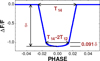 |
Fig. 1. Simplified transit shape used in this paper. The flux drops linearly in the ingress and egress parts at a rate given by the T14/T12 ratio and δ. The U-shaped bottom is supposed to model the overall limb darkening. It has an analytical form of |
Single outliers. We recall that no outlier selection is made in the data processing up to the pre-BLS phase. Since the BLS search is sensitive to outliers, we focus on these, while carefully avoiding cases when transit-like features are suspected. As a result, we consider only those instances when the flux decrease is limited to the middle point among three successive points. The outlier status is determined on the basis of the deviation from the average of the two fluxes left and right of the point of interest. If this deviation exceeds 3σ0 (with σ0 being the sigma-clipped standard deviation of the pre-BLS phase time series), then the flux of this point is replaced by the flux average of the neighboring points. A similar procedure can be employed in the reconstruction phase, when the transit signal helps further identifying the single outliers.
Flare correction. In a non-negligible number of stars, flares may also jeopardize the success of the search for periodic transits, since these events increase the colored-noise component of the BLS spectrum. Here, we resorted the simplest and far from optimum way to remedy the effect of flares. By considering only events of flux increase relative to the average or to a given transit signal – depending on the stage of the analysis – we replace the “positive” outliers by the average or the corresponding values of the transit signal. We do not correct any “flare” that does not exceed the 3σ0 limit as given above.
3.1. Detuned Fourier fit
To handle stellar variability, we opted for traditional Fourier decomposition, whereby – based on very fundamental and well-known properties of Fourier series defined on a finite interval – we can fit the smooth part of the observed flux variation. Even though any stellar variability has an inherently stochastic component (primarily due to surface convection), the adjacent fluxes are correlated to some degree and the variation appears to be continuous (albeit non-periodic). Consequently, we can apply Fourier decomposition for a very large class of variations. Even though this is true, we have to be aware of the fact that the finite timebase inevitably introduces discontinuities, and as such, induce what is commonly known Gibbs oscillations close to the edges of the dataset. Minimizing this oscillatory behavior is obviously a crucial step since these high-frequency oscillations can easily dominate the time series after corrections for systematics and stellar variability.
To avoid any data loss by simply chopping off some fraction of both ends of the dataset, we searched for various methods in the literature devoted to Gibbs oscillation minimization (e.g., by using the Lanczos sigma factor8). Because we did not find a suitable one, we tested the idea of period detuning (a method we did not find in the literature we reviewed). Although a precise discussion of the method is beyond the scope of this paper, we illustrate the method at work on an example. The idea is simple: to increase the fundamental period (and its harmonics) to some extent and thereby push the oscillations outside the timebase of interest.
We show the effect of detuning in Fig. 2. We generated a sinusoidal signal on the observed timebase of one of the members of Campaign 5. We chose the following parameters: P = 7.6508 d, A = 10 ppt (parts per thousand, i.e., A = 0.010), with an additive Gaussian (white) noise of σ = 0.001 ppt. We set the order of the Fourier fit equal to 50. We see that detuning works very efficiently, with only a negligible overshooting close to the noise level. The degree to which detuning may eliminate the Gibbs phenomenon depends on the type of signal and the order of the Fourier series. Nevertheless, the method has worked neatly in nearly all cases encountered so far during the analysis of the 20 000 stars of Campaign 5.
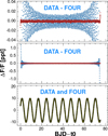 |
Fig. 2. Illustration of the effect of frequency detuning with fixed frequency components {fi = (i + 1)/(β × T)}, where T is the total time span and β = 1.0 for the classical Fourier decomposition (steelblue dots) and β = 1.05 for the detuned case (brown dots). Lower panel: input sinusoidal signal (black line) and the Fourier fit (yellow line – there is no β dependence on this scale). |
3.2. Autoregressive edge correction
Here, we focus on those (not very numerous) cases when detuning does not work. Instead of trying to adjust the Fourier order, we opted to employ an AR model on the noise-perturbed Fourier fit and predict the Gibbs-free signal at the edges. The AR modeling is always performed and compared with the Fourier fit and the one is chosen that yields a better fit to the data. The main steps of the AR modeling are as follows.
First we cut some fraction (L data points, some 5% the full set of N points) of the Fourier signal at the edges of the dataset. We add Gaussian noise to the signal to avoid complete fit to the Fourier solution and, thereby, reproduce the Gibbs oscillations at the edges, where the AR model is used to predict the oscillation-free continuation of the Fourier solution. The size of the noise can be estimated from the fit based on the Fourier model.
Second, we interpolate the above noisy Fourier signal {x(i);i = 1, 2, …, n} to an equidistant timebase and fit it by a high-order AR model. To maintain stability, we use an AR order of m = 900. To determine the autoregressive coefficients {aj}, we use one-side predictions for the outermost m data points, that is,
for the left and the right ends, respectively. For the middle of the dataset (i.e., from k = m + 1 to k = n − m), we use a two-side model with simple arithmetic mean,
![$$ \begin{aligned} x(k) = {1 \over 2} \sum _{i=1}^m a_{i}[x(k+i) + x(k-i)] . \end{aligned} $$](/articles/aa/full_html/2020/11/aa38726-20/aa38726-20-eq10.gif)
Least squares with equal weights are used to determine the AR coefficients {ai}.
Third, we predict the outermost L values of the Fourier points from those interior to the edges. We found that these predictions may still have some curvature or mild wavy behavior. To eliminate this feature, and protect any possible transit feature close to the end points, we robustly fit 5th-order polynomials to the AR predictions.
Finally, we compare the residuals between the systematics-free data and approximations obtained by the AR and Fourier modeling. Select the one that yields smaller Root Mean Square (RMS) and pass the so-obtained systematics- and variability-free time series to the BLS routine.
To illustrate the method at work, we generated a synthetic sinusoidal signal with P = 9.091 d, semi-amplitude A = 500 ppt and superposed a transit signal with Ptr = 14.286 d, δ = 0.2 ppt. We also added two individual boxy transits near the end points to test if the method would preserve these events. The order of the Fourier series is 50. The result is shown in Fig. 3. It is important to note that the Fourier fit was done with a detuned fundamental period (see Sect. 3.1). As emphasized earlier in this paper, detuning is very efficient in eliminating the Gibbs oscillations. If detuning is not efficient enough, AR modeling may come to the rescue and allow for the detection of faint signals.
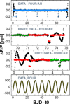 |
Fig. 3. Illustration of the elimination of the Gibbs oscillations at the edges of the dataset by using AR modeling. Bottom: input dataset (black line: noisy sinusoidal with transits), Fourier fit (yellow). Transits are not visible at this scale. Middle panels: residual signal after subtracting the best Fourier fit and the best AR model (black and red dots, respectively). The green dots indicate where the Fourier fit was accepted. Uppermost panel: residual time series obtained by Fourier (black) and AR modeling (light blue). See text for the main signal parameters. |
3.3. TFA template selection
The selection of the proper set of cotrending time series is one of the fundamental issues in filtering out systematics from the observed signal. The most liberal choice is to avoid obvious variables showing excessive scatter, while otherwise not paying too much attention to stellar variability in the cotrending set (i.e., Kovacs et al. 2005). The somewhat vague (but, under certain circumstance, functional) argument here is that in the presence of noise and targeting transits, the variability of the cotrending time series will be scaled down due to the nearly constant nature of the target time series. The transits, due to their short time scales will not be substantially affected and the final result will be positive since the cotrending time series will fit primarily the systematics due to their coherence with regard to these components in the flux variation of the target. Interestingly, this approach has been fairly successful over the numerous applications in searching for periodic transits.
In spite of the success of the “brute force” method described above, efforts have been made to decrease the number of cotrending time series as much as possible to: (a) avoid signal degradation due to overfitting: (b) using only the essential (i.e., “most common”) components and striving towards a better separation of the transit signal and systematics. The most obvious approach in reaching these goals is to employ PCA on the pre-selected set of candidate cotrending time series and use only those components that are “essential”, based on their PCA eigenvalues. From the very first application in the SysRem algorithm by Tamuz et al. (2005), this selection method has been widely used, often supplemented by other criteria, such as selecting dominant components from the PCA set based on the statistical properties of the regression coefficients of the cotrending vectors (Petigura & Marcy 2012). Or, in another approach, application of maximum likelihood criterion by considering the effect of the non-Gaussian nature of the full model with systematics (i.e., PDC-MAP, the Kepler pipeline by Smith et al. 2012; Stumpe et al. 2012).
Because the Kepler data are dominated by systematics, rather than white noise (at least down to the Neptune/super-Earth regime); here, we recognize the importance of avoiding variables in the TFA templates set. However, we still do not use any PCA-like combination to select the “most dominant” correcting vectors. This is because templates that are “less common” could also be useful in certain cases. For example, outlier data points may lead to the rejection of a particular template in the PCA classification, whereas the same template may become rather instrumental in filtering out these outlying points if and when they occur in a target of interest. This is very important since the signal of interest (the transit) is also some sort of outlier. Preserving the transit but treating the outliers “naturally” (i.e., without clipping them) is an important ingredient of a successful transit (or transient) search.
The main steps in selecting the TFA template set are as follows:
-
Spatially uniform sampling: Because systematics are different across the field of view (FOV), we aim for spatially homogeneous sampling. From each of the 19 tiles (built up from 2 × 2 closely spaced CCD units) we select the same number of templates. Because of the distortion introduced by the use of equatorial coordinates (α, δ), we shifted, rotated and stretched or squeezed the FOV so that all the tiles took approximately the shape of a rectangle. This step is necessary for the simple bookkeeping of the potential templates and their association with a given tile. The transformation formulae to the new coordinate system (X, Y) are as follows:
We determined the transformation parameters with a simple trial and error method. For C05, we obtained: α0 = 130.2, δ0 = 16.8, ω = −1°. In each tile, the potential templates were chosen from a uniform random distribution on the brightness-ordered list of stars. We allowed up to 200 random tries from each tile and selected those stars that satisfied the criteria below:
-
Focus on low photon noise: Templates are chosen from the bright side of the magnitude distribution of the campaign field (in the case of C05, this limit was set at Kp = 13.4, corresponding the brightest 10 000 stars in the field).
-
Avoid near singular cases: The distance between two template stars should exceed some value, dmin, limited by the PSF of the Kepler telescope.
-
Small overall scatter: The RMS of the residuals around the fitted low-order polynomial {p} to the SAP time series {x} cannot be greater than σt, i.e., σ(x/p) < σt.
-
Small Fourier power: The Fourier fit {f} to the residuals of the polynomial fit above should not improve the goodness of fit by more than a factor of rσ, that is, σ(x/p)/σ(x/p − f) < rσ.


We used 2nd order polynomials and 50th order Fourier series in all template sets. These parameters were chosen after various tests, including visual inspection of the candidate templates. The other parameters resulted from the same procedure, and set at the following values: σt = 0.03 (in relative flux units, normalized to 1.0 in respect of the average flux of the given star), rσ = 1.2. The final set of templates is shown in Fig. 4. It is intriguing that the tile in the center contains significantly less number of templates than all the other tiles. A brief visual examination of the light curves (LCs) for this tile revealed an overall lower level of satellite rotation adjustment. As suggested by the referee of this paper, the different behavior of the objects on the central tile could be related to the closeness of this tile to the rotation axis of the satellite. However, the general drift and the ramping at the start of the campaign remained, leading to a poor polynomial fit at low order. Consequently, the Fourier fit on the residuals became more significant and that led to the failure in satisfying the “small Fourier power” criterion by most of the LCs associated with this tile. Although the template number distribution among the tiles can be made uniform easily by using a higher order polynomial fit, this does not change the detection efficacy in any major way (i.e., all detections discussed in this paper remain reliable).
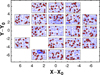 |
Fig. 4. Distribution of the TFA template stars (red dots) for 387 templates. The X and Y coordinates (given in [deg] relative to the center of the field) result from the transformation of the equatorial coordinates to remedy strong distortions of the CCD subfields (see text). The best-fitting rectangles to the hulls of the subfields are shown by black lines. The small blue dots show the stars with Kepler photometry. |
3.4. Optimizing the Fourier order
The determination of the Fourier order NFOUR is important because in critical cases (e.g., in the presence of high-frequency or high-amplitude stellar flux variations), the shallow transit signal can be easily washed out by an overly high-order fit or by leaving in the high-frequency components because of an overly parsimonious choice of the Fourier order. Due to the complexity of the time series, in addition to the specific representation of it via a Fourier series with frequencies independent of the actual contributing components, standard methods (e.g., Fisher test) for optimized parameter number are cannot be straightforwardly employed. The method presented here is far from exact. It is largely based on the general pattern of the root mean square (RMS) of the Fourier fit as a function of the number of the Fourier components (in brief the Fourier order). The scheme and the parameters used are derived form the large number of tests performed on the Campaign 5 data and serve only a single purpose: to separate the smooth Fourier component from the discrete transit events.
It is also important to investigate whether testing the SAP LCs is suitable for a reliable estimation of the best Fourier order. We found that systematics may lead to serious errors in the estimated order. Therefore, we decided to perform a TFA filtering first and then employ the method described below on the filtered data to estimate the Fourier order.
The main goals of the optimization are as follows: to (i) find a simple and easy to use criterion that handles most cases of stellar variabilities encountered in the Kepler survey; (ii) minimize mixing instrumental systematics and stellar variability; (iii) perform the determination of the optimum order quickly (before the complex filtering of the input time series, involving systematics and stellar variability); (iv) aim for low Fourier order (CPU demand increases sharply by higher Fourier order).
All these point towards a pursuit of low-order fits and we restrict this search to NFOUR < 150. Concerning point (iii) above, we linearly interpolate the TFA-filtered LC of the target to an equidistant basis and perform the test by using simple Fourier transforms (equivalent to a least squares fit on an equidistant timebase, but much faster).
As expected, σ(NFOUR) – that is, the RMS of the residuals of the fit – has a very steep decreasing part for low NFOUR and then, a long, nearly linearly decreasing tail toward higher NFOUR values. If there is a high-frequency stellar variation, then we have other steep drops in RMS at large-enough NFOUR values. The nearly flat parts in the σ(NFOUR) function make the simple Fisher test difficult to use for parameter optimization. Therefore, the method described below considers both the statistical properties of the RMS of the Fourier fit and the possible late (i.e., high NFOUR) convergence of the fit.
The steps for the determination of the optimum Fourier order are as follows.
(a) Fit the SAP LC with the TFA template set to be used by the routine performing the full analysis for the target. Use the residuals of this fit in the subsequent steps.
(b) Compute σ(NFOUR) for NFOUR = 1 − 150 by omitting 5% of the data points at both edges (to avoid extra increase in RMS due to the Gibbs phenomenon).
(c) Perform robust linear fit to σ(NFOUR) between NFOUR = 100 and 150.
(d) Compute S1, the RMS of the above linear fit.
(e) Extrapolate this line all the way to the lowest Fourier order, and compute the difference ΔL between σ(NFOUR) and the extrapolated line L(NFOUR). The first type of optimum Fourier order M1 is defined as the largest order at which σ − L is greater than S1.
(f) Compute the ratio R2(NFOUR) = σ2(NFOUR)/σ150, where σ150 is the standard deviation of σ2(NFOUR) at the highest Fourier order tested, i.e.,  , where n is the original number of data points with a factor taking into account the data cut at the edges (see above)9. The second type of optimum Fourier order M2 is defined as the largest order at which R2(NFOUR) − R2(150) > 6.
(g) Since we found too low order fits often insufficient, the optimum Fourier order is defined as follows: Mopt = MAX(20, MIN(M1, M2)+10).
Figure 5 exhibits four typical types of the functions described above. The examples shown come from the list of planetary candidates of Kruse et al. (2019). The uppermost panel shows the pattern for an apparently non-variable star. As expected, the optimum Fourier order is low. The R2 statistic shows a similar pattern. Since R2 gives the change in σ2(NFOUR) normalized to its theoretical error at the highest Fourier order tested, the absolute value of the change in R2 is important. This is different from the statistic derived from the linear fit to the tail of σ(NFOUR), which yields a measure of only the topological property of the RMS variation.
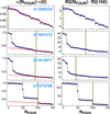 |
Fig. 5. Examples on the optimized selection of the Fourier order. Left column: normalized standard deviation of the Fourier fit as a function of the Fourier order. Red line shows the robust linear regression to the data in NFOUR = 100 − 150. Right column: fit variances over the standard deviation of the fit variance at NFOUR = 150. Vertical yellow stripes show the optimum Fourier orders derived from the statistics given in the header. See text for further details. |
The next panel shows the case where the size of the stellar variability is similar to the size of the systematics. The robust fit and the interval chosen to perform the linear regression leads to a bad approximation of the low-NFOUR regime, reflecting the trend expected from the high-NFOUR regime, where the harmonic content of the signal is supposed to be exhausted. The point where the prediction deviates by more than a given amount (see above) yields an estimate of the minimum Fourier order. Similarly, the R2 statistic measures the relative change, and when it exceeds a certain amount, we can consider that value of NFOUR as the minimum value needed to represent the Fourier content of the signal.
The other two examples are dominated by stellar variability. The target in the bottom panel is a good example for the stepsize variation of σ(NFOUR) and the need to map this function to rather high values. From the rule given in the last step of the optimization process, from top to bottom, Fourier orders that were ultimately applied are as follows: 20, 86, 53, and 110.
To illustrate the overall performance of the code and the validity of the optimized choice of the Fourier order, Figure 6 shows the case of EPIC 211897272. The quasi-periodic stellar variability has been well disentangled from the systematics and resulted in the detection of the transit signal with a depth of 0.5 ppt (some 40-times smaller than the amplitude of the SAP signal, heavily scrambled by systematics in the first half of the campaign).
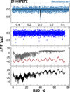 |
Fig. 6. Example of the capability of joint robust Fourier and TFA fit in disentangling stellar variability and measurement systematics. The target name and the type of the final data product are indicated in the header. The Fourier order is optimized at NFOUR = 83. From the bottom to top: raw (SAP) LC from KEP; TFA and FOUR components; raw minus (TFA+FOUR) components – the periodic dips due to the transit signal emerge; folded LC with the best BLS period. Continuous black line: best fitting transit signal. |
In summary, to avoid excessive run times by using flat, overestimated Fourier order for all targets (and risk losing some of the important candidates because of overfitting), optimization seems to be an important part of the data processing. We found that well over 90% of the potential candidates can be found in this way and we get signatures of hidden signals for the remaining few percents. These targets can be resolved by performing more detailed tests, including the sensitivity of the detection against changing the Fourier order.
4. Significance of the signal reconstruction (complete signal modeling)
When unknown signal components are searched without the exact knowledge of the perturbing components, it is unavoidable that some deformation in the signal that is searched for will be introduced. This is simply because of the (natural) incompleteness of the model we use for a signal search. This effect is present even when using some “protective shield” for the unknown component, such the self-adjusted weights on outliers used in this paper. There have been attempts to avoid signal degradation that is due to the use of incomplete signal models (Foreman-Mackey et al. 2015; Angus et al. 2016; Taaki et al. 2020), but a subsequent work by Kovacs et al. (2016) showed that full modeling in a signal search is considerably less efficient than previously considered, and, obviously, more demanding in terms of CPU power.
Although the overall accuracy is always a focus of attention in deriving parameters of interest in any physical system, certain parameters may bear a greater importance. In the particular case of extrasolar planets, the radius (through the scaleheight) is a crucial parameter in planetary atmosphere models and it is obviously important in population synthesis studies. For example, the “radius gap” problem (the low number density of planets at Rp ∼ 2REarth ; see, e.g. Van Eylen et al. 2018; Fulton & Petigura 2018) is quite sensitive to the radius error, which should be pushed below 5% to sharpen the feature needed for further theoretical considerations (Petigura 2020).
Constituting the last step of the signal search, reconstruction requires the knowledge of the signal period and the approximate parameters of the transit. By adding this approximation to complete the signal model, we can iteratively improve the signal parameters by solving this complete model (see Kovacs et al. 2005, for the first application of this approach). Here, we use Eq. (6) supplied by the successive approximations of the transit signal to minimize Eq. (5) with the optimized weights {w(i)}. We note in passing that full modeling is a must in most cases for a precise transit parameter determination and is used commonly in planet atmosphere studies based on space observatory data such as HST and Spitzer (Knutson et al. 2008).
In the following, we investigate the signal preserving properties of TRAN_K2 from injected signal tests performed on a subset of field C05. Because of the substantial size of the parameter space, we simplify the test to all transit parameters fixed, except for the transit depth, which is our main focus of interest. In preparing the tests, first we define our detection parameters and criteria.
4.1. Signal detection parameters
We consider the signal detected in a simulation if all criteria below are satisfied:
-
|1 − Pobs/Pinj| < 0.002
-
δ < 0
-
S/Nsp > 6 with S/Nsp = (sp(peak)− < sp > )/σ(sp).
Here Pobs denotes the observed period at the peak power of the BLS spectrum of the time series with the injected test signal of period Pinj. The second condition filters out possible flares, whereas the third one is our standard condition to characterize the signal to noise ratio (S/N) of the BLS spectrum (sp(peak), < sp> and σ(sp), respectively, stand for the peak value, the average, and the standard deviation of the spectrum). The search was performed in the frequency band [1/T, 2.5] c/d, where the lower limit comes from the constraint of avoiding large gaps in the trial phase-folded LCs at periods longer than the total time span T. To minimize low-frequency power surplus (Bakos et al. 2004), the spectrum was robustly fitted by a 6th-order polynomial and the residuals were used to compute S/Nsp.
Although in the particular case of test signals we did not use any other parameters to characterize the significance of the signal, in the transit survey performed on the field of C05, we also utilized the quantity we call spectral peak density (SPD). This parameter is aimed at attaining a quantification of the sparsity of the spectrum, yielding small values for those with few large peaks and large values for those with many small ones. The former spectra are more likely to contain significant signal, whereas the latter ones look more closely to what we expect from a noise. For further reference, SPD is defined as follows:
where N(sp/sp(peak) > spcut) is the number of spectral values (normalized to the highest peak) exceeding a certain cutoff from the available N(sp) spectral points. When trained on the C05 data, we found that spcut = 0.3 yields a quite reliable estimate of the “cleanliness” of the spectra and the derived SPD values are consonant with the visual inspections.
Although S/Nsp and SPD yield useful information on the signal content of the time series, the quality of the derived folded light curve may not always entirely in agreement with the scores received from these parameters. This is because spectral parameters reflect the relative significance of the peak component to other possible components. For example, in the case of rare or single – otherwise high-S/N – events, S/Nsp and SPD will, in general, indicate low significance, whereas the folded LC will obviously suggest the presence of a strong signal. Therefore, largely following Kovacs et al. (2005), we characterize the quality of the folded LC by the dip significance parameter (DSP):
where |δ| is the absolute value of the transit depth, varδ is the variance of the average (i.e., square of the error of the mean) of the intransit data points (i.e., all points from the first contact to the last one). In the evaluation of the remaining variances we divide the phase-folded LC into bins of the same length as the full transit10. By omitting the bin corresponding to the transit, we compute the bin averages for the Nb out of transit (oot) bins {aoot(j);j = 1, 2, …, Nb}. The variance of these values is varoot. This quantity may not decrease DSP to the level needed in the case of ragged LCs with large variations between the oot bins. Therefore, we added the average of the squared differences between the adjacent bin averages, that is,  .
.
4.2. Tests: transit depth and transit duration
As we mentioned earlier in this section, we limit the tests on signals that differ only in transit depth, with all other parameters fixed during each simulation. Two types of transit signal are used, namely:
Signal A:Ptr = 11.111 d, T14 = 0.2 d, T12/T14 = 0.2, 0.1 < |δ| < 1.9 ppt, no sinusoidal component.
Signal B: Signal A with a sinusoidal component; period: 7.692 d, amplitude: 20 ppt.
We note that the center of transit and the phase of the sinusoidal component are not important in the present context. The transit depth δ is chosen from a uniform distribution. The range of transit depth was chosen to roughly match most of the values of the candidates in the list of Kruse et al. (2019).
We used our “400” TFA template set of 387 stars with low stellar variability from the PET database, and injected the signals above. These signals were tested with and without employing the reconstruction option. We focus on the transit depth and duration in the comparison of the injected and derived parameters.
From the 387 injected signals of type A, we recovered 297. For type B injections, the rate was slightly lower (294). Figure 7 shows the ratio of the detected and injected values for δ and T14. We see that with signal reconstruction the derived basic transit parameters are essentially unbiased, however, with its scatter increasing toward signals of lower significance. Also, except perhaps for the transit duration, there is no difference (in statistical sense) between the parameters derived from signals with or without a sinusoidal component.
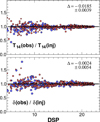 |
Fig. 7. Ratio of the observed and injected transit depths δ and durations, T14, as functions of the dip significance parameter DSP. Transit parameters have been derived by using signal reconstruction. Red and blue points show the result with (signal B) and without (signal A) added sinusoidal component to mimic stellar variability. Inset labels show the mean differences and their errors for signal A. The estimated transit parameters show no overall bias. |
On the other hand, without employing complete signal model, we get a substantial bias (Fig. 8). As expected, the observed transit depths are lower than the injected values, with a strong increase in this difference toward less significant signals. The transit duration follows the same same pattern, albeit the bias is somewhat lower.
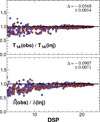 |
Fig. 8. As in Fig. 7, but without employing signal reconstruction. The estimated transit parameters show significant bias, especially for less significant signals at lower DSP values. |
The above tests give supporting evidence that TRAN_K2 is capable of yielding unbiased estimates of the basic transit parameters, assuming that a complete signal model is used. We expect that, in general, transit depth and duration are estimated better than ∼10% for strong (DSP > 12) signals. For weaker signals, the errors increase, but they are unlikely to go above ∼30% while simultaneously maintaining the unbiased nature of the estimates.
5. Comparison with other searches
Before we compare the detection rates between our search by TRAN_K2 and other searches, we present the averages of the standard deviations of the means, taken on a 6.5 hour timebase of our final data product (i.e., including signal reconstruction). This quantity, often referred to as a combined differential photometric precision (CDPP, Christiansen et al. 2012), is devoted to evaluating the potential of transit detection based solely on the overall error of the means on a given (transit) timescale. There are various approximations for this quantity (e.g., Vanderburg & Johnson 2014; Aigrain et al. 2016), which often include the application of a Savitsky-Golay-type (i.e., least squares polynomial) filtering of the final data product (e.g., Gilliland et al. 2011; Luger et al. 2018). Here, we relied on the full time series model and computed the 6.5 hour CDPP from the unbiased estimate of the standard deviation (σfit) of the residuals between the model and the input time series. With the overall cadence of 0.5 hours, we get CDPP(6.5)  . For the ∼20 000 stars analyzed, we obtained the result shown in Fig. 9.
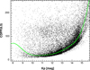 |
Fig. 9. Average of the standard deviations of the 6.5 hour means (in parts per million) vs. stellar brightness. The final time series (i.e., the full, reconstructed models) were used to calculate the standard deviations from the residuals between these and the input (raw) time series. The continuous line shows the robust fit of a 10th order polynomial to the data. |
For the updated EVEREST pipeline, Luger et al. (2018) report basically a full agreement for the ridge CDPP values with those of the original Kepler mission. Vanderburg & Johnson (2014), in their Table 1, compare the CDPP values of SFF with those of the original Kepler mission. From this table we have 18, 22, 30, and 81 ppm precision at Kp = 10.5, 11.5, 12.5, and 14.5, respectively. From the ridge fit to the CDPP values in Fig. 9. we have 20, 23, 32, and 89 ppm at these magnitude values. In spite of the impressive close approximation of the precision of the original Kepler mission, we caution that low CDPP values tell only that the residuals are small at the particular window used, but it does not automatically grant a powerful transit detection. This depends on the delicate balance between noise suppression and transit signal preservation.
One of the basic steps in testing the code performance is to verify earlier detections and check the consistency of the transit parameters. Although this is obviously an important way for both human and machine training searches as well as a crucial test for the comparison of the detection efficacy of different methods, there are two caveats to keep in mind before making too far-reaching conclusions based on such a test: (i) the result may depend on the input time series (SAP photometry) that are obtained differently by various groups; (ii) the detection criteria and thoroughness of the analysis might vary between the different searches, namely, discarding the trace of transit in one search and considering it in another.
Focusing only on Campaign 5, in the basic verification, we relied primarily on the 115 host stars with 138 planet candidates of Kruse et al. (2019). In addition to this quite recent work, we also tested the 8 candidates in Zink et al. (2020). The basic analysis was performed on the PET database, but in unresolved cases, we also used the KEP database.
From the 115 targets of Kruse et al. (2019), 103 have been identified with high confidence by using the survey setting of the code (i.e., optimized Fourier order with detection criteria listed in Sect. 4.1). The remaining 12 targets were examined in detail. By using the KEP data, 7 of these were reclassified as “good or strong” detections. EPIC 211613886 showed up as a high S/N candidate in both datasets, but with half of the period given by Kruse et al. (2019). Therefore, we accepted it as a “detection.” EPIC 211988320 shows multiple, apparently non-repetitive transit events, yielding high S/N detection, but the favored period is different from the one given by Kruse et al. (2019). Because of the non-repetitive nature of the events and the significance of events, we consider this candidate as “detected”. The case of EPIC 211939692 is quite similar, but the Fourier order is overestimated, yielding a lower S/N. A detailed examination showed that with a lower Fourier order, this target comes out as strong as EPIC 211988320. Finally, we are left with only two candidates (EPIC 211432922 and 211913395) that we could not detect, no matter how hard we tried (which is in agreement with the conclusion reached at the various earlier stages while developing TRAN_K2).
It is an obvious matter of interest to compare the basic transit parameters derived in this study and those of Kruse et al. (2019). Figure 10 shows the result of this comparison. In the light of the tests presented in Sect. 4.2, it is quite surprising to see the systematic difference and the large scatter between the two studies. To add to this discrepancy, the injected signal test performed by Zink et al. (2020) indicates that the EVEREST transit depths are lower by some 2.3% as they should be. Unfortunately, we have no answer at this moment on the source of the apparently significant discrepancy between our results and those of Kruse et al. (2019).
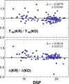 |
Fig. 10. Comparison of the transit depth δ and transit duration T14 between this work (KO) and that of Kruse et al. (2019) (KR). The 103 targets detected from the analysis of the PET dataset are plotted. The mean differences and their errors are shown in the upper right corners. |
Interestingly, while testing their planet vetting pipeline on C05, Zink et al. (2020) found eight candidates that do not enter in the list of Kruse et al. (2019). At the same time, they could not verify 49% of the candidates of Kruse et al. (2019). Considering that both studies are based on EVEREST data (however, appended with different analysis tools and vetting criteria), this is quite intriguing and shows the delicacy of planet search in the strongly contaminated environment of stellar variability and instrumental systematics.
In checking the candidates of Zink et al. (2020), we found three targets confirmed with high S/N. The fourth planet candidate in EPIC 211562654 is confirmed. For EPIC 211711685, we found a single event in addition to the component claimed by Zink et al. (2020). EPIC 212119244 was also confirmed, albeit with low S/N at twice of the period given by Zink et al. (2020). There remained two candidates (EPIC 211953244 and 212020330) that we could not confirm, in spite of extensive testing.
6. Search for new candidates
Although the field of C05 has been scrutinized in numerous searches (Barros et al. 2016; Pope et al. 2016; Mayo et al. 2018; Petigura et al. 2018; Kruse et al. 2019; Zink et al. 2020), we decided to do the same, based on the high success rate in identifying the already known candidates. With the goal of presenting a secure list of new candidates for potential followup studies, we surveyed the brightest 20 000 stars from the nominally available ∼25 000 targets. The analysis was run on the KEP and PET datasets separately. The signal search was performed in the frequency interval of [0, 3] c/d. We used the “400” template sets for the respective datasets and the optimization method for selecting the Fourier order.
The most viable candidates were selected by using the following detection criteria: S/Nsp > 7, SPD < 0.5, δ < 0, DSP > 5, Nev > 1, T12/T14 < 0.3 and Nev/Nint < 0.5. The first two conditions simply require that the BLS spectrum be of high-S/N and sparse enough, as expected from the spectrum of a transit signal embedded in moderate to tolerable noise. The next two conditions require that the folded signal should imply flux decrease and also be of reasonably significant. The next condition makes avoidance of single transits (nevertheless, we found a nice one, likely at an earlier stage of search, when such a criterion was not employed). To decrease the binary false positive rate, we added the condition of minimum steepness of the ingress and egress phases. Finally, to avoid false detections due to repeating outliers, we required the transit be reasonably well covered by the individual events (i.e., the number of transit events should be considerably smaller than the number of intransit data points). Clearly, this might lead to missing some candidates with transit durations of less than an hour or so.
For the simplest way of linearly decreasing the total running time on our multiprocessor computer, the data were analyzed parallel in segments containing 5000 stars in each set. The selection criteria above yielded 233, 127, 83 and 39 items from these sets containing objects of decreasing brightness (and, consequently, of higher noise). These pre-selected targets were then more deeply inspected and then selected as viable candidates if the inspections and tests (e.g., stability of the signal against changing the Fourier order, sensitivity to the selection of the TFA template set) ended up positive. Then we deselected those candidates that were already suggested by the surveys listed above. Thereafter, a brief check of the physical plausibility of the detected companion was made on the basis of the published stellar parameters from recent large-scale studies, aided by the Gaia satellite. The top candidates were then further examined for additional transit components.
We found 15 candidates11 passing all these steps and ending up as potential planetary systems. The derived photometric transit parameters for these systems are given in Table 1, the accompanying diagnostic plots are shown in Appendix A.
New planetary candidates from K2 Campaign 5.
By using the stellar parameters accessible through Gaia DR2 (Gaia Collaboration 2018) along with the TESS and the K2 stellar catalogs (Huber et al. 2016; Stassun et al. 2019; Hardegree-Ullman et al. 2020), we checked the physical properties of the new candidate systems. As a sanity check, assuming central transit and circular orbit, we computed the relative transit duration Qtran = T14/Porb through the basic stellar parameters and orbital period:
where the stellar parameters are in solar units, the period is in days. We note that this check does not depend on the blending status of the target.
In testing the consistency of the calculated transit durations with the observed ones, first we selected systems with a well-established planetary status (see Appendix B, Table B.2). Then, we plotted the corresponding Qtran values together with those of the new candidates. Figure 11 shows that the new candidates presented in this paper fit well into the overall topology of this plot: most of the systems lack exact central transit, therefore, the calculated Qtran values are greater than the observed values12. Several systems have Qtran(calc) < Qtran(obs). The most likely cause of this discrepancy is the insufficient accuracy of the stellar parameters. Another, albeit less likely or efficient contributing factor is orbital eccentricity. The most prominent downward outlier was WASP-4 (Wilson et al. 2008). All current stellar radius values are in the close neighborhood of 0.90 R/R⊙ (Bonfanti & Gillon 2020), making it difficult to increase the calculated Qtran value. High-resolution imaging (Bergfors et al. 2013) does not indicate any nearby companion that might indirectly affect the transit duration.
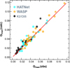 |
Fig. 11. Observed vs. calculated relative transit durations for the 15 systems presented in this paper, together with the 30 HATNet and 30 WASP planetary systems detailed in Appendix B. Equation (16) was used to derive Qtran(calc). The surplus of objects above the 45° line indicates the expected effect of off-central transit. The slight excess of systems below the 45° line is due to errors in the stellar masses and radii. |
In the evaluation of the candidates, we estimated the planet radii with the assumption that blending was not an issue for any of the targets. The stellar and planetary parameters are summarized in Table B.1 of Appendix B.
We found that the majority of the companions have radii between 1 and 2 Earth radii. We have five candidates (EPIC 211537406, 211777794, 211825799, 211977277, and 211503363) with sub-Jupiter–Neptune radii. Except for EPIC 211537406, in this group of more massive planets, all companions are around evolved (off of the main sequence) stars.
The brightest candidate, EPIC 211914045 is special in our sample. The star is a K dwarf and the companion has a sub-Earth radius of 0.63 RE. The candidate was detected only in the KEP time series. This can be the result of the optimized aperture used by the KEP pipeline. The PET time series are generated by K2PHOT with an aperture size of 3 × 3 pixels. The corresponding square covers the target and avoids gathering photons from the considerably fainter stars about 10″ to the North13. The exact location and the extent of the optimized aperture of the KEP pipeline is not known, but the net flux is higher by some 5% than the one supplied by K2PHOT. This may indicate some level of contamination by the neighbors. Our fully processed LC for the KEP data yields RMS = 0.053 ppt, while for the LC derived from the PET data we get 0.061 ppt. The higher precision is a likely contributing factor to the detection in the KEP data. No time series are available for the faint visual double to the North, but the nearby, similarly bright star EPIC 211913753 to the South, show no signal in any of the databases. Because of the lack of full-frame images with sufficient cadence during the K2 campaigns, we can rely only on future dedicated followup works to decide if the faint neighbors to the North have any contribution to the signal detected in EPIC 211914045.
We searched for additional planets both among the 115 systems of Kruse et al. (2019) and the newly found 15 systems. As described in Sect. 3, we successively subtracted the already found transit component, and searched for the next one until the S/N of the spectrum reached the noise level. In the final solution all transit components were included together with the stellar variation and instrumental systematics. The transit depths were fitted simultaneously, with the other transit parameters fixed. Naturally, the search for additional components is also sensitive to secondary eclipses and, therefore, it helps in filtering out false positives. We did not find any sign for blended binaries among the candidate systems.
Altogether, we found five systems that were classified either as single or of lower multiplicity. Somewhat more detailed description of the systems follows below. The parameters of transit components are given in Table 2.
New planetary candidates in multiple systems from K2 C05.
EPIC 211314705. This is a three-planet candidate. There is no entry in Kruse et al. (2019); listed as a single-planet candidate in Pope et al. (2016). We found two additional signals with transit depths ∼1.5 and 1.2 ppt. Somewhat intriguingly, the orbital periods have a constant ratio of 1.38. Figure 12 shows the BLS spectra and the folded LCs for the three components.
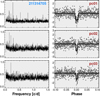 |
Fig. 12. Three-planet candidate EPIC 211314705. Left panels: successively prewhitened BLS spectra, normalized to unity at each panel. The spectra are divided into 2000 bins and only the maxima are shown in each bin. Right panels: folded LCs for each component, zoomed on the transit. Continuous line shows the fit to our transit model. Relative fluxes are in [ppt]. |
EPIC 211562654. This is K2-183, a five-planet candidate. It is entered as a 3-planet candidate in Kruse et al. (2019). The fourth component was discovered by Zink et al. (2020). Here, we present the fifth component, in near 2:1 resonance with the fourth component. The transit center of the fifth candidate is located at Tc(4)+0.375P4, indicating that it is not some sort of artifact of the method used during the prewhitening of pc04. The ratio of the relative transit durations is not entirely consonant with the expected value from Eq. (16), but is still within the error range indicated by our tests for a signal of DSP ∼ 9 (see Fig. 7). The five components are displayed in Fig. 13.
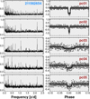 |
Fig. 13. Five-planet candidate EPIC 211562654. Notation is the same as in Fig. 12. The short-period component pc03 may exhibit TTV, as indicated by the high power remained at the same frequency in the BLS spectrum of panel pc05 and the proximity of the associated epoch to that of pc03. |
EPIC 212012119. This is a three-planet system, listed by both Pope et al. (2016) and Kruse et al. (2019) as a two-planet system. The third component is in a near 3:1 resonance with the second component. The transit center of the third component is near in the middle of the three-period cycle of the second component, that is, Tc(2)+1.482P2. The observed decrease in the transit length is greater than expected from Eq. (16), but again, this is within the error limits. The three components are displayed in Fig. 14.
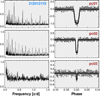 |
Fig. 14. Three-planet candidate EPIC 212012119. Notation is the same as in Fig. 12. The third candidate is in a close 3:1 resonance with the second candidate. |
EPIC 212164470. This is a two-planet system, listed earlier as a single component system by Pope et al. (2016) and Kruse et al. (2019). The two components are displayed in Fig. 15.
EPIC 211988320. This is a likely multiplanetary system, but the orbital periods are not well constrained because of the rareness of the transit events. Kruse et al. (2019) list this target as a single planet system, but as shown in Fig. 16, the system must host more than one planet.
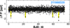 |
Fig. 16. Time series of the multiplanet candidate EPIC 211988320. The orbital periods are not well constrained because of the rareness of the transit events (shown with yellow background shading for better visibility). The time series starts at t0 = 2457139.6111. |
7. Conclusions
In an effort to test some simple ideas in further improving our capability to detect shallow transits in the environment of dominating colored noise, we developed TRAN_K2, a standalone Fortran code. Development and debugging were performed on the Campaign 5 field data of the K2 mission, including the direct use of these data together with various test signals injected into the original data. The input data were the raw (simple aperture photometry) fluxes available in public archives.
The input signal is assumed to be built up from four components: (i) instrumental systematics; (ii) stellar variability; (iii) white noise; (iv) transit signal. In filtering out (i), we used cotrending (TFA), based on low-variability stars in the field and some image property parameters. To eliminate the effect of (ii), we used Fourier modeling.
The prime goal was to protect the underlying transit signal from being crushed during the pre-BLS phase and thereby to ensure a maximum S/N for the resulting frequency spectrum. To reach this goal, we employed the following ingredients in the pre-BLS data preparation.
-
We used a general Fourier series representation of the stellar variability (i.e., without knowing the particular signal frequencies entering in the few-parameter model of the signal).
-
To minimize the overshoots due to the Gibbs phenomenon at the edges of the dataset, we employed detuned fundamental frequency in the Fourier series and autoregressive modeling near the edges.
-
To protect the sharp transit features, data-adapted weighting was used in the robust least squares fit of the combination of the Fourier and TFA parts of the model. No outliers were selected at this stage.
-
After the above TFA+Fourier filtering, the data were corrected for single outliers and flares before passing them to the BLS search.
Except for single events, the BLS spectrum represents the basic statistic that determines whether the found signal is interesting or not. Although the S/N of the peak remains the prime indicator of the signal content, we found it useful to introduce the spectral peak density (SPD) that characterizes the sparseness of the spectrum.
A final step in the signal analysis is to consider all signal constituents, including the transit components found in the BLS search. In this grand robust fit, we get a considerable improvement on the precision of the transit depths, which is a vital parameter in planet characterization and also prone to underestimation when the modeling is incomplete.
We found that TRAN_K2 is capable of detecting nearly all previously claimed systems and planet components, with a missing rate of 1 − 2%. We found that the strength of the detections depends, at a non-negligible level, on the input data used. In particular, the database from the standard Kepler pipeline and the one produced by K2PHOT often result in spectra of different quality and, therefore, occasionally, missing candidates in one of these datasets.
In spite of the several earlier visits of Campaign 5 by various groups, we found 15 new candidate systems and 5 additional planets in already known planetary systems. A brief check made on the physical size of the new planet candidates indicate that most of them have radii less than 2 RE and there is one candidate with Rp = 0.6 RE.
By following the jargon of the developers of the Kepler post-processing pipeline (see Smith et al. 2012; Stumpe et al. 2012), we often use the word “cotrending” for this filtering process.
The Gibbs phenomenon is an asymptotic property of the Fourier decomposition, and follows from the “almost everywhere” type of convergence for square-integrable functions – e.g., for continuous functions defined on finite intervals. It is often exhibited as high-frequency oscillations or overshootings if the order of the Fourier decomposition is high enough.
AR modeling performs backward/forward prediction from the linear combination of certain number of future/past values of a time series (see Sect. 3.2 and Fahlman & Ulrych 1982; Caceres et al. 2019, for early, and recent applications).
The formula cited for the standard deviation of the sample variance is valid under the assumption that the residuals follow a Gaussian distribution. For an easy reference, see: https://stats.stackexchange.com/questions/29905/reference-for-mathrmvars2-sigma4-left-frac2n-1-frac-kappan
Acknowledgments
This project would not be possible without our new powerful servers. We are indebted to the IT management of the Observatory (including Noémi Harnos, Mihály Váradi and Evelin Bányai) for the careful installation and the prompt (and positive) response to our requests. Waqas Bhatti from the Department of Astrophysical Sciences of the Princeton University is gratefully acknowledged for the essential pieces of advice in matters concerning these servers. This paper includes data collected by the Kepler mission. Funding for the Kepler mission is provided by the NASA Science Mission directorate. This research has made use of the VizieR catalogue access tool, CDS, Strasbourg, France (DOI: 10.26093/cds/vizier). Supports from the National Research, Development and Innovation Office (grants K 129249 and NN 129075) are acknowledged.
References
- Aigrain, S., Parviainen, H., & Pope, B. J. S. 2016, MNRAS, 459, 2408 [NASA ADS] [Google Scholar]
- Alapini, A., & Aigrain, S. 2009, MNRAS, 397, 1591 [NASA ADS] [CrossRef] [Google Scholar]
- Alonso, R., Brown, T. M., Torres, G., et al. 2004, ApJ, 613, L153 [NASA ADS] [CrossRef] [Google Scholar]
- Angus, R., Foreman-Mackey, D., & Johnson, J. A. 2016, ApJ, 818, 109 [NASA ADS] [CrossRef] [Google Scholar]
- Bakos, G., Noyes, R. W., Kovács, G., et al. 2004, PASP, 116, 266 [NASA ADS] [CrossRef] [Google Scholar]
- Bakos, G. Á., Torres, G., & Pál, A. 2010, ApJ, 710, 1724 [NASA ADS] [CrossRef] [Google Scholar]
- Barros, S. C. C., Demangeon, O., & Deleuil, M. 2016, A&A, 594, A100 [NASA ADS] [CrossRef] [EDP Sciences] [Google Scholar]
- Bergfors, C., Brandner, W., Daemgen, S., et al. 2013, MNRAS, 428, 182 [NASA ADS] [CrossRef] [Google Scholar]
- Bonfanti, A., & Gillon, M. 2020, A&A, 635, A6 [CrossRef] [EDP Sciences] [Google Scholar]
- Caceres, G. A., Feigelson, E. D., Jogesh Babu, G., et al. 2019, AJ, 158, 57 [CrossRef] [Google Scholar]
- Christiansen, J. L., Jenkins, J. M., Caldwell, D. A., et al. 2012, PASP, 124, 1279 [NASA ADS] [CrossRef] [Google Scholar]
- Deming, D., Knutson, H., Kammer, J., et al. 2015, ApJ, 805, 132 [NASA ADS] [CrossRef] [Google Scholar]
- Fahlman, G. G., & Ulrych, T. J. 1982, MNRAS, 199, 53 [NASA ADS] [CrossRef] [Google Scholar]
- Foreman-Mackey, D., Montet, B. T., Hogg, D. W., et al. 2015, ApJ, 806, 215 [NASA ADS] [CrossRef] [Google Scholar]
- Fulton, B. J., & Petigura, E. A. 2018, AJ, 156, 264 [Google Scholar]
- Gaia Collaboration (Brown, A. G., et al.) 2018, A&A, 616, A1 [NASA ADS] [CrossRef] [EDP Sciences] [Google Scholar]
- Gilliland, R. L., Chaplin, W. J., Dunham, E. W., et al. 2011, ApJS, 197, 6 [NASA ADS] [CrossRef] [Google Scholar]
- Hardegree-Ullman, K. K., Zink, J. K., Christiansen, J. L., et al. 2020, ApJS, 247, 28 [CrossRef] [Google Scholar]
- Huber, D., Bryson, S. T., Haas, M. R., et al. 2016, ApJS, 224, 2 [NASA ADS] [CrossRef] [Google Scholar]
- Knutson, H. A., Charbonneau, D., Allen, L. E., et al. 2008, ApJ, 673, 526 [NASA ADS] [CrossRef] [Google Scholar]
- Kovacs, G. 2017, Eur. J. Web Conf. Phys, 01005 [CrossRef] [Google Scholar]
- Kovacs, G. 2018, A&A, 614, L4 [NASA ADS] [CrossRef] [EDP Sciences] [Google Scholar]
- Kovacs, G., Zucker, S., & Mazeh, T. 2002, A&A, 391, 369 [NASA ADS] [CrossRef] [EDP Sciences] [Google Scholar]
- Kovacs, G., Bakos, G., & Noyes, R. W. 2005, MNRAS, 356, 557 [NASA ADS] [CrossRef] [Google Scholar]
- Kovacs, G., Hartman, J. D., & Bakos, G. A. 2016, A&A, 585, 57 [CrossRef] [EDP Sciences] [Google Scholar]
- Kovács, G., & Kovács, T. 2019, A&A, 625, A80 [NASA ADS] [CrossRef] [EDP Sciences] [Google Scholar]
- Kruse, E., Agol, E., Luger, R., et al. 2019, ApJS, 244, 11 [CrossRef] [Google Scholar]
- Luger, R., Agol, E., Kruse, E., et al. 2016, AJ, 152, 100 [Google Scholar]
- Luger, R., Kruse, E., Foreman-Mackey, D., et al. 2018, AJ, 156, 99 [NASA ADS] [CrossRef] [Google Scholar]
- Mayo, A. W., Vanderburg, A., Latham, D. W., et al. 2018, AJ, 155, 136 [NASA ADS] [CrossRef] [Google Scholar]
- McCullough, P. R., Stys, J. E., Valenti, J. A., et al. 2005, PASP, 117, 783 [NASA ADS] [CrossRef] [Google Scholar]
- Petigura, E. A. 2020, AJ, 160, 89 [CrossRef] [Google Scholar]
- Petigura, E. A., & Marcy, G. W. 2012, PASP, 124, 1073 [NASA ADS] [CrossRef] [Google Scholar]
- Petigura, E. A., Schlieder, J. E., Crossfield, I. J. M., et al. 2015, ApJ, 811, 102 [Google Scholar]
- Petigura, E. A., Crossfield, I. J. M., Isaacson, H., et al. 2018, AJ, 155, 21 [NASA ADS] [CrossRef] [Google Scholar]
- Poddany, S., Brat, L., & Pejcha, O. 2010, New Astron., 15, 297 [NASA ADS] [CrossRef] [Google Scholar]
- Pollacco, D. L., Skillen, I., Collier Cameron, A., et al. 2006, PASP, 118, 1407 [NASA ADS] [CrossRef] [Google Scholar]
- Pope, B. J. S., Parviainen, H., & Aigrain, S. 2016, MNRAS, 461, 3399 [Google Scholar]
- Smith, J. C., Stumpe, M. C., Van Cleve, J. E., et al. 2012, PASP, 124, 1000 [Google Scholar]
- Southworth, J., Bohn, A. J., Kenworthy, M. A., et al. 2020, A&A, 635, A74 [NASA ADS] [CrossRef] [EDP Sciences] [Google Scholar]
- Stassun, K. G., Oelkers, R. J., Paegert, M., et al. 2019, AJ, 158, 138 [Google Scholar]
- Stumpe, M. C., Smith, J. C., Van Cleve, J. E., et al. 2012, PASP, 124, 985 [Google Scholar]
- Taaki, J. S., Kamalabadi, F., & Kemball, A. J. 2020, AJ, 159, 283 [CrossRef] [Google Scholar]
- Tamuz, O., Mazeh, T., & Zucker, S. 2005, MNRAS, 356, 1466 [NASA ADS] [CrossRef] [Google Scholar]
- Vanderburg, A., & Johnson, J. A. 2014, PASP, 126, [Google Scholar]
- Van Eylen, V., Agentoft, C., Lundkvist, M. S., et al. 2018, MNRAS, 479, 4786 [Google Scholar]
- Wilson, D. M., Gillon, M., Hellier, C., et al. 2008, ApJ, 675, L113 [NASA ADS] [CrossRef] [Google Scholar]
- Zink, J. K., Hardegree-Ullman, K. K., Christiansen, J. L., et al. 2020, AJ, 159, 154 [CrossRef] [Google Scholar]
Appendix A: New candidates
We show the diagnostic plots for the 15 new planetary candidate systems presented in Sect. 6. All candidates are in the Campaign 5 field of the K2 mission. Please consult with Sect. 6 (Table 1) and Appendix B (Table B.1) for details of the system parameters and physical properties.
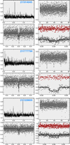 |
Fig. A.1. Diagnostic plots for the new candidates. Clock-wise for each star: BLS spectrum, time series, zoomed and full phase-folded light curves. For the zoomed light curve the residuals (data minus model) are shifted upward for better visibility. Transit model: Black line. Y axis units: arbitrary (BLS), ppt (others). X axis units: d−1 (BLS), BJD−2457139.610425 (time series), phase (others). |
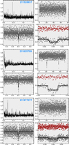 |
Fig. A.2. Diagnostic plots for the new candidates. See Fig. A.1 for details. Candidates no. 4–6 from Table 1 are plotted. |
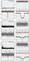 |
Fig. A.3. Diagnostic plots for the new candidates. See Fig. A.1 for details. Candidates no. 7–9 from Table 1 are plotted. |
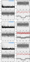 |
Fig. A.4. Diagnostic plots for the new candidates. See Fig. A.1 for details. Candidates no. 10–12 from Table 1 are plotted. |
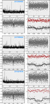 |
Fig. A.5. Diagnostic plots for the new candidates. See Fig. A.1 for details. Candidates no. 13–15 from Table 1 are plotted. |
Appendix B: Predicted and estimated transit durations
To support Fig. 11 here, we present the actual values used to create the plot. For completeness, we also include the coordinates and the planet radii for the new K2/C05 candidates.
Table B.1 shows the basic stellar parameters for the 15 new candidates. The stellar parameters are the simple averages of the values published by the Gaia Collaboration (Gaia Collaboration 2018), those given in the K2 and TESS Input Catalogs (Huber et al. 2016; Stassun et al. 2019), and the items of a revised K2 catalog by Hardegree-Ullman et al. (2020). Depending on the availability, we could use between two and four values to calculate the averages. For EPIC 211528937 Huber et al. (2016) yields a factor of two larger radius, therefore, their item is omitted for this target. For the single transiter EPIC 211503363, we used P = 58 d (the minimum period). We note that this table is aimed primarily at the estimation of the transit duration from the stellar parameters and orbital period and it may not pass the rigor usually followed in the analysis of newly discovered individual systems. Nevertheless, the consistency of the stellar parameters from various catalogs gives enough trust in the estimated transit durations and planetary radii.
Some parameters of the new planetary candidates presented in this paper.
Table B.2 contains the main stellar parameters and Qtran values for the first 30 extrasolar planetary systems discovered by the two major wide-field ground-based surveys. The stellar parameters are from the TESS Input Catalog (TIC, see Stassun et al. 2019). The transit durations based on TIC have been proven to be more accurate than those calculated with the aid of14 – the calculated Qtran values were less frequently lower than the observed values. The observed transit durations were gathered from the Exoplanet Transit Database (ETD; see Poddany et al. 2010). As before, Eq. (16) was used to derive Qcalc.
Sample of confirmed planets for the transit duration test.
The sequential numbers of the WASP systems are not continuous, because WASP-9 was proven to be a false positive, WASP-11=HAT-P-10 and WASP-27=HAT-P-14. We also note that WASP-30b is not a planetary system, but a stellar binary, with a near main-sequence F8 primary and a 61 MJ secondary, that can be classified as a brown dwarf. Because there is no mass entry in TIC for WASP-20, we relied on the analysis of Southworth et al. (2020). WASP-20 is a binary, and the stellar parameters correspond to the brighter companion.
All Tables
All Figures
|
Fig. 1. Simplified transit shape used in this paper. The flux drops linearly in the ingress and egress parts at a rate given by the T14/T12 ratio and δ. The U-shaped bottom is supposed to model the overall limb darkening. It has an analytical form of |
| In the text | |
|
Fig. 2. Illustration of the effect of frequency detuning with fixed frequency components {fi = (i + 1)/(β × T)}, where T is the total time span and β = 1.0 for the classical Fourier decomposition (steelblue dots) and β = 1.05 for the detuned case (brown dots). Lower panel: input sinusoidal signal (black line) and the Fourier fit (yellow line – there is no β dependence on this scale). |
| In the text | |
|
Fig. 3. Illustration of the elimination of the Gibbs oscillations at the edges of the dataset by using AR modeling. Bottom: input dataset (black line: noisy sinusoidal with transits), Fourier fit (yellow). Transits are not visible at this scale. Middle panels: residual signal after subtracting the best Fourier fit and the best AR model (black and red dots, respectively). The green dots indicate where the Fourier fit was accepted. Uppermost panel: residual time series obtained by Fourier (black) and AR modeling (light blue). See text for the main signal parameters. |
| In the text | |
|
Fig. 4. Distribution of the TFA template stars (red dots) for 387 templates. The X and Y coordinates (given in [deg] relative to the center of the field) result from the transformation of the equatorial coordinates to remedy strong distortions of the CCD subfields (see text). The best-fitting rectangles to the hulls of the subfields are shown by black lines. The small blue dots show the stars with Kepler photometry. |
| In the text | |
|
Fig. 5. Examples on the optimized selection of the Fourier order. Left column: normalized standard deviation of the Fourier fit as a function of the Fourier order. Red line shows the robust linear regression to the data in NFOUR = 100 − 150. Right column: fit variances over the standard deviation of the fit variance at NFOUR = 150. Vertical yellow stripes show the optimum Fourier orders derived from the statistics given in the header. See text for further details. |
| In the text | |
|
Fig. 6. Example of the capability of joint robust Fourier and TFA fit in disentangling stellar variability and measurement systematics. The target name and the type of the final data product are indicated in the header. The Fourier order is optimized at NFOUR = 83. From the bottom to top: raw (SAP) LC from KEP; TFA and FOUR components; raw minus (TFA+FOUR) components – the periodic dips due to the transit signal emerge; folded LC with the best BLS period. Continuous black line: best fitting transit signal. |
| In the text | |
|
Fig. 7. Ratio of the observed and injected transit depths δ and durations, T14, as functions of the dip significance parameter DSP. Transit parameters have been derived by using signal reconstruction. Red and blue points show the result with (signal B) and without (signal A) added sinusoidal component to mimic stellar variability. Inset labels show the mean differences and their errors for signal A. The estimated transit parameters show no overall bias. |
| In the text | |
|
Fig. 8. As in Fig. 7, but without employing signal reconstruction. The estimated transit parameters show significant bias, especially for less significant signals at lower DSP values. |
| In the text | |
|
Fig. 9. Average of the standard deviations of the 6.5 hour means (in parts per million) vs. stellar brightness. The final time series (i.e., the full, reconstructed models) were used to calculate the standard deviations from the residuals between these and the input (raw) time series. The continuous line shows the robust fit of a 10th order polynomial to the data. |
| In the text | |
|
Fig. 10. Comparison of the transit depth δ and transit duration T14 between this work (KO) and that of Kruse et al. (2019) (KR). The 103 targets detected from the analysis of the PET dataset are plotted. The mean differences and their errors are shown in the upper right corners. |
| In the text | |
|
Fig. 11. Observed vs. calculated relative transit durations for the 15 systems presented in this paper, together with the 30 HATNet and 30 WASP planetary systems detailed in Appendix B. Equation (16) was used to derive Qtran(calc). The surplus of objects above the 45° line indicates the expected effect of off-central transit. The slight excess of systems below the 45° line is due to errors in the stellar masses and radii. |
| In the text | |
|
Fig. 12. Three-planet candidate EPIC 211314705. Left panels: successively prewhitened BLS spectra, normalized to unity at each panel. The spectra are divided into 2000 bins and only the maxima are shown in each bin. Right panels: folded LCs for each component, zoomed on the transit. Continuous line shows the fit to our transit model. Relative fluxes are in [ppt]. |
| In the text | |
|
Fig. 13. Five-planet candidate EPIC 211562654. Notation is the same as in Fig. 12. The short-period component pc03 may exhibit TTV, as indicated by the high power remained at the same frequency in the BLS spectrum of panel pc05 and the proximity of the associated epoch to that of pc03. |
| In the text | |
|
Fig. 14. Three-planet candidate EPIC 212012119. Notation is the same as in Fig. 12. The third candidate is in a close 3:1 resonance with the second candidate. |
| In the text | |
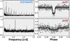 |
Fig. 15. Two-planet candidate EPIC 212164470. Notation is the same as in Fig. 12. |
| In the text | |
|
Fig. 16. Time series of the multiplanet candidate EPIC 211988320. The orbital periods are not well constrained because of the rareness of the transit events (shown with yellow background shading for better visibility). The time series starts at t0 = 2457139.6111. |
| In the text | |
|
Fig. A.1. Diagnostic plots for the new candidates. Clock-wise for each star: BLS spectrum, time series, zoomed and full phase-folded light curves. For the zoomed light curve the residuals (data minus model) are shifted upward for better visibility. Transit model: Black line. Y axis units: arbitrary (BLS), ppt (others). X axis units: d−1 (BLS), BJD−2457139.610425 (time series), phase (others). |
| In the text | |
|
Fig. A.2. Diagnostic plots for the new candidates. See Fig. A.1 for details. Candidates no. 4–6 from Table 1 are plotted. |
| In the text | |
|
Fig. A.3. Diagnostic plots for the new candidates. See Fig. A.1 for details. Candidates no. 7–9 from Table 1 are plotted. |
| In the text | |
|
Fig. A.4. Diagnostic plots for the new candidates. See Fig. A.1 for details. Candidates no. 10–12 from Table 1 are plotted. |
| In the text | |
|
Fig. A.5. Diagnostic plots for the new candidates. See Fig. A.1 for details. Candidates no. 13–15 from Table 1 are plotted. |
| In the text | |
Current usage metrics show cumulative count of Article Views (full-text article views including HTML views, PDF and ePub downloads, according to the available data) and Abstracts Views on Vision4Press platform.
Data correspond to usage on the plateform after 2015. The current usage metrics is available 48-96 hours after online publication and is updated daily on week days.
Initial download of the metrics may take a while.