| Issue |
A&A
Volume 642, October 2020
|
|
|---|---|---|
| Article Number | A46 | |
| Number of page(s) | 20 | |
| Section | Extragalactic astronomy | |
| DOI | https://doi.org/10.1051/0004-6361/202038009 | |
| Published online | 07 October 2020 | |
The halo of M 105 and its group environment as traced by planetary nebula populations
I. Wide-field photometric survey of planetary nebulae in the Leo I group⋆
1
European Southern Observatory, Karl-Schwarzschild-Str. 2, 85748 Garching, Germany
e-mail: This email address is being protected from spambots. You need JavaScript enabled to view it.
2
European Southern Observatory, Alonso de Cordova 3107, Vitacura, Casilla 19001, Santiago de Chile, Chile
3
Max-Planck-Institut für Extraterrestrische Physik, Giessenbachstraße, 85748 Garching, Germany
4
Excellence Cluster Universe, Boltzmannstraße 2, 85748 Garching, Germany
5
Research School of Astronomy & Astrophysics Mount Stromlo Observatory, Cotter Road, 2611 Canberra, Australia
6
School of Physics and Astronomy, University of Nottingham, Nottingham NG7 2RD, UK
7
Departamento de Astronomia, Instituto de Astronomia, Geofisica e Ciencias Atmosfericas da USP, Cidade Universitaria, 05508900, Sao Paulo, Brazil
8
Leiden Observatory, Leiden University, PO Box 9513, 2300 RA Leiden, The Netherlands
Received:
24
March
2020
Accepted:
17
July
2020
Abstract
Context. M 105 (NGC 3379) is an early-type galaxy in the Leo I group. The Leo I group is the nearest group that contains all main galaxy types and can thus be used as a benchmark to study the properties of the intra-group light (IGL) in low-mass groups.
Aims. We present a photometric survey of planetary nebulae (PNe) in the extended halo of the galaxy to characterise its PN populations and investigate the presence of an extended PN population associated with the intra-group light.
Methods. We use PNe as discrete stellar tracers of the diffuse light around M 105. These PNe were identified on the basis of their bright [O III]5007 Å emission and the absence of a broad-band continuum using automated detection techniques. We compare the PN number density profile with the galaxy surface-brightness profile decomposed into metallicity components using published photometry of the Hubble Space Telescope in two halo fields.
Results. We identify 226 PNe candidates within a limiting magnitude of m5007, lim = 28.1 from our Subaru-SuprimeCam imaging, covering 67.6 kpc (23 effective radii) along the major axis of M 105 and the halos of NGC 3384 and NGC 3398. We find an excess of PNe at large radii compared to the stellar surface brightness profile from broad-band surveys. This excess is related to a variation in the luminosity-specific PN number α with radius. The α-parameter value of the extended halo is more than seven times higher than that of the inner halo. We also measure an increase in the slope of the PN luminosity function at fainter magnitudes with radius.
Conclusions. We infer that the radial variation of the PN population properties is due to a diffuse population of metal-poor stars ([M/H] < −1.0) following an exponential profile, in addition to the M 105 halo. The spatial coincidence between the number density profile of these metal-poor stars and the increase in the α-parameter value with radius establishes the missing link between metallicity and the post-asymptotic giant branch phases of stellar evolution. We estimate that the total bolometric luminosity associated with the exponential IGL population is 2.04 × 10⁹ L⊙ as a lower limit. The lower limit on the IGL fraction is thus 3.8%. This work sets the stage for kinematic studies of the IGL in low-mass groups.
Key words: galaxies: individual: M 105 / galaxies: elliptical and lenticular, cD / galaxies: groups: individual: Leo I / galaxies: halos / planetary nebulae: general
Based on data collected at Subaru Telescope, which is operated by the National Astronomical Observatory of Japan under programme S14A-006 and with the William Herschel Telescope operated on the island of La Palma by the Isaac Newton Group of Telescopes in the Spanish Observatorio del Roque de los Muchachos of the Instituto de Astrofísica de Canarias.
© ESO 2020
1. Introduction
In a cold dark matter (CDM) dominated Universe with a cosmological constant (ΛCDM), structure forms hierarchically (White & Rees 1978; Peebles 1980). In this paradigm, the favoured formation scenario for early-type galaxies (ETGs) is a two-phase process: the initial phase of strong in situ star formation (e.g. Thomas et al. 2005, and references therein) is followed by growth through mergers and accretion (White & Frenk 1991; Steinmetz & Navarro 2002; Oser et al. 2010). Therefore, the study of the distribution and kinematics of stars in their extended halos can provide important constraints on late galaxy growth, as accretion events leave behind long-lasting dynamical signatures in the velocity phase-space (e.g. Bullock & Johnston 2005; Richardson et al. 2008; Starkenburg et al. 2009; Helmi et al. 2011; Crnojević et al. 2016) as well as low-surface brightness features such as stellar streams, fans, and plumes (e.g. Ferguson et al. 2002; Mihos et al. 2005, 2017; Belokurov et al. 2007; Janowiecki et al. 2010; Longobardi et al. 2015a).
The galaxy M 105 (NGC 3379) has long been regarded as a prototypical ETG to be described by the classic de Vaucouleurs surface brightness profile (de Vaucouleurs & Capaccioli 1979). Later, M 105 was at the centre of a long-standing debate on the dark matter (DM) content of ETGs and is one of the poster children of the Planetary Nebula Spectrograph (PN.S) ETG survey (Douglas et al. 2007). Using data obtained with the PN.S, Romanowsky et al. (2003) and Douglas et al. (2007) found that several intermediate-luminosity elliptical galaxies, one of which is M 105, appeared to have low-mass and low-concentration DM halos, if any, on the basis of their rapidly falling velocity dispersion profiles. Follow-up studies argued that this apparent lack of dark matter might be due to anisotropy and viewing-angle effects (Romanowsky et al. 2003; Dekel et al. 2005; de Lorenzi et al. 2009). Similarly, Schwarzschild modelling based on SAURON integral-field spectroscopic data was also consistent with a DM halo and non-negligible radial anisotropy (Weijmans et al. 2009).
M 105 is not an isolated galaxy but is situated in a group environment. The Leo I group, named initially G11 group, in which M 105 resides, is the nearest loose group to contain both early- and late-type massive galaxies (de Vaucouleurs 1975). The group contains at least 11 bright galaxies and has an on-sky extent of 1.6 × 1.0 Mpc (de Vaucouleurs 1975). Of the 11 bright galaxies, 7, including M 105, are associated with the M 96 (NGC 3368) group, and the remaining 4 are associated with the so-called Leo Triplet. The Leo I group is rich in dwarf galaxies: Müller et al. (2018) recently discovered 36 new candidates in a 500 square-degree volume in addition to the previously known 52 dwarf galaxies.
The group is surrounded by a segmented ring with a diameter of 200 kpc that consists of neutral hydrogen (Schneider et al. 1983). After its discovery, Schneider (1985) showed that the kinematics of the H I gas could be reconciled with an elliptical orbit centred at the luminosity-weighted centroid of M 105 and the nearby NGC 3384 spiral galaxy. In their model, the ring rotates with a period of approximately 4 Gyr. However, the crossing times in the group are much shorter than this (Pierce & Tully 1985), which is problematic for the stability of the ring. Moreover, only the disc of NGC 3384 is aligned with the orientation of the ring, which is puzzling if M 105, NGC 3384, and M 96 formed from a single rotating cloud. An alternative formation scenario to the primordial origin of the H I ring is the collision of two spiral galaxies (Rood & Williams 1984, 1985). A recent simulation of the collision of two gaseous disc galaxies reproduces both the shape and rotation of the H I ring and the lack of a visible-light counterpart (Michel-Dansac et al. 2010).
There is no evidence for low surface brightness (LSB) features associated with the H I ring and for an extended diffuse intra-group light (IGL) out to the HI ring, brighter than the surface brightness (SB) limit of μB = 30 mag arcsec (Watkins et al. 2014). Furthermore, Castro-Rodríguez et al. (2003) did not detect any PNe associated with the H I ring and set an upper limit of  on the IGL fraction, that is, on the fraction of light attributed to the IGL with respect to the light from group galaxies. These findings contradict the results from numerical simulations, which predict that galaxy groups have IGL fractions between 12% and 45% (Sommer-Larsen 2006; Rudick et al. 2006). However, Watkins et al. (2014) argued that galaxies in the Leo I group fall below the mass resolution of the simulations mentioned above, and we might thus expect a correspondingly dimmer IGL component. If this was the case, Watkins et al. (2014) argued that the IGL would still contribute a few percent at most towards the total light in the group.
Harris et al. (2007a) found evidence for a metal-poor (MP) halo at ∼12 Reff based on deep and high spatial resolution Hubble Space Telescope (HST) photometry in the western halo of M 105. Their Advanced Camera for Surveys (ACS) field seems to lie at the transition radius where the MP red giant branch (RGB) population starts to dominate the metal-rich (MR) one. Both populations are inferred to have ages of 12 Gyr and metallicities of [M/H] < −0.7 and [M/H] ≥ −0.7, respectively. Lee & Jang (2016) combined these data with an archival HST ACS pointing in the very inner halo at approximately 3 Reff south-east from the centre of M 105. In their independent analysis, they corroborated the existence of two distinct subpopulations both in colour and metallicity: a dominant, red, MR population with an approximately solar peak metallicity, and a much weaker, blue, MP population whose peak metallicity is [M/H]≈ − 1.1. The average ages and metallicities in the inner halo agree with those inferred by Weijmans et al. (2009), who found a stellar population consistent with a metallicity slightly below 20% solar metallicity (≈ − 0.7 dex) and an age of 12 Gyr.
The origin of this extended MP halo is still a subject of debate. Harris et al. (2007a) ruled out a single chemical evolution sequence for the halo stars. Instead, they proposed a multi-stage formation model: the MP halo was built up first from pristine gas, and the star formation therein was truncated approximately at the time of cosmological reionisation. The MR, bulge-like component was formed later from pre-enriched gas and with a higher yield, eventually resulting in the observed solar abundances. Lee & Jang (2016) also suggested a two-phase formation model for the halo in which the red and MR halo was formed in situ or through the major mergers of massive progenitors, while the blue and MP halo was formed through dissipationless mergers and accretion.
Using extended photometric and kinematic samples of planetary nebulae (PNe), we aim to place better constraints on the assembly history of M 105 and its group environment. Our new PN data span a minor-axis distance that is three times larger than that of Douglas et al. (2007). This will place valuable new constraints on the stellar populations in the outer halo as traced by PNe, and on the PN spatial and line-of-sight (LOS) velocity distributions of the M 105 stars at large radii.
This paper is the first in a series and is organised as follows. In Sect. 2 we present the photometric and kinematic surveys of PNe in the Leo I group. In Sect. 3 we review the results from broad-band photometric surveys. We then study the relation between the azimuthally averaged distribution of the PNe and the SB photometry in Sect. 4. In Sect. 5 we evaluate the constraints from the resolved stellar populations and relate their physical parameters to the observed properties of the PN sample in M 105. Section 6 covers the PN luminosity function (PNLF) of M 105 and its variation with radius. We conclude this paper with a discussion in Sect. 7. Paper II in this series will focus on the dynamics of the M 105 halo and the Leo I group.
In the remainder of this paper, we adopt a physical distance of 10.3 Mpc to M 105 from surface brightness fluctuation measurements (SBF; Tonry et al. 2001), which agrees well with the tip of the red giant branch (TRGB) distance independently determined by Harris et al. (2007a, b) and Lee & Jang (2016). The corresponding physical scale is 49.6 pc/″. The effective radius of M 105 has been determined to be  , which corresponds to a physical radius of 2.7 kpc (Capaccioli et al. 1990). The structural parameters of M 105 relevant to this paper are summarised in Table 1.
Properties of M 105 and NGC 3384 based on broad-band photometry.
2. Photometric and kinematic surveys of PNe in the Leo I group
The photometric and kinematic surveys in this work expand our ongoing effort to study PNe as tracers in group and cluster environments. We combine kinematic data from the extended PN.S (ePN.S) ETG survey (Arnaboldi et al. 2017; Pulsoni et al. 2018), including two additional newly acquired fields, with accurate narrow- and broad-band photometry obtained with SuprimeCam mounted at the prime focus of the 8.2 m Subaru telescope (Miyazaki et al. 2002). In what follows, we focus on the results from our SuprimeCam survey and use the ePN.S data set as an independent validation of the PN candidates from the SuprimeCam data. A detailed analysis of the more extended kinematic PN survey will be discussed in Paper II of this series.
2.1. Subaru SuprimeCam photometry
2.1.1. Survey description and data reduction
We used the on-off band technique to detect PNe candidates in M 105. The pointing centred on M 105 was observed through a narrow-band [O III] filter (λc, on = 5029 Å, Δλon = 74 Å) and a broad-band V-filter (λc, off = 5500 Å, Δλoff = 956 Å), using the same observational strategy as Longobardi et al. (2013), who observed M 87 in the Virgo cluster. The observations were taken in the same night as those of Hartke et al. (2017) in their survey of M 49. We therefore only briefly recapitulate the data reduction steps and refer to Hartke et al. (2017) for further details.
In order to reach fluxes in [OIII] that are two magnitudes fainter than the PNLF bright cut-off ( , assuming an absolute bright cut-off of the PNLF of M⋆ = −4.51, Ciardullo et al. 2002), six dithered exposures with a total exposure time of 1.8 h through the on-band and six dithered exposures with a total exposure time of 0.6 h through the off-band filter were observed. The observing conditions were photometric, with seeing better than
  . The photometric zero-points were calculated to be Z[O III],AB = 24.51 ± 0.04 and ZV, AB = 27.48 ± 0.01 by Hartke et al. (2017). To convert AB magnitudes into m5007 magnitudes from the [O III] line, we used the relation derived by Arnaboldi et al. (2003) for the SuprimeCam narrow-band filter,
 (1)
(1)
The relation between integrated flux F5007 and magnitude m5007 is given by the Jacoby relation (Jacoby 1989),
 (2)
(2)
The data were reduced using the instrument pipeline SDFRED21. As the field is dominated by the three bright and extended galaxies M 105, NGC 3384, and NGC 3398, the final images were astrometrised and stacked with the tools Weight Watcher (Marmo & Bertin 2008), SCAMP (Bertin 2006), and SWARP (Bertin et al. 2002) from the astromatic software suite. We used the UCAC-4 catalogue (Zacharias et al. 2012) as an astrometric reference. To determine the point-spread functions (PSFs) of the images, we used the psf task of the IRAF-daophot2 package. The best-fit PSF profile is a Moffat function with  , seeing radius rFWHM = 2.35 pix (corresponding to
  ), and axial ratio b/a = 0.96.
2.1.2. Selection of PN candidates and catalogue extraction
To select PN candidates, we made use of the characteristic spectral features of PNe: a bright [O III]5007 Å emission line and no significant continuum emission. Observed through the on-band filter, PNe appear as unresolved sources at extragalactic distances, while they are not detected in the off-band image. Arnaboldi et al. (2002, 2003) developed a CMD-based automatic selection procedure that selects PNe based on their excess in [O III]–V colour and their point-like appearance. This technique has since been tailored to SuprimeCam data by Longobardi et al. (2013) and Hartke et al. (2017). For reference, the detailed catalogue extraction procedure for M 105 can be found in Appendix A.
The limiting magnitude of our survey is defined as the magnitude at which the recovery fraction of a simulated PN population extracted from our images falls below 50% (see Appendix A.2). We extracted 226 objects within a limiting magnitude of m5007, lim = 28.1 and therefore cover 2.6 mag from the bright cut-off of the PNLF m⋆ = 25.5 mag. We further discuss the nature of the PNLF of M 105 in Sect. 6. Our survey covers 67.6 kpc (23 effective radii) along the major axis of M 105 and also covers the halos of NGC 3384 and NGC 3398. The selected PN candidates are denoted as blue crosses in Fig. 1.
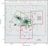 |
Fig. 1. DSS image of M 105. Overplotted are the PN candidates from the Subaru survey (blue crosses), PNe from the ePN.S survey (Pulsoni et al. 2018, green pluses), and the e2PN.S survey (this work, red pluses and crosses). PNe in NGC 3384 from Cortesi et al. (2013a) are denoted with green circles. The red and green rectangles denote the ePN.S and e2PN.S fields, and the dashed blue rectangle indicates the SuprimeCam footprint. The grey hatched regions indicate the two HST fields analysed in Lee & Jang (2016). The scale bar in the lower right corner denotes 10 kpc. North is up, and east is to the left. |
2.2. Extended Planetary Nebula Spectrograph (ePN.S) ETG survey
The PN.S is a custom-built double-arm slitless spectrograph mounted at the William Herschel Telescope (Douglas et al. 2002). Its design enables the identification of PNe and the measurement of their LOS velocities in a single observation. The ePN.S ETG survey (Arnaboldi et al. 2017; Pulsoni et al. 2018) provides positions (RA, Dec), LOS velocities (v), and magnitudes (m5007, PN.S) for spatially extended samples of PNe in 33 ETGs. The survey typically extends out to 6 effective radii (re).
2.2.1. M 105 (NGC 3379)
M 105 was one of the first ETGs observed with the PN.S and was a milestone for the development of the PN.S data reduction pipeline (Douglas et al. 2007). As part of the PN.S ETG survey (Douglas et al. 2007), 214 PNe were observed, covering a major-axis distance of 5.3 Reff. These are indicated by green pluses in Fig. 1.
2.2.2. NGC 3384
As the on-sky distance between M 105 and the SB0-galaxy NGC 3384 is only 435″ and the difference in distance modulus between the galaxies is only 0.2 mag, their PN populations appear superimposed. An immediate separation in velocity space is not possible due to the small difference in systemic velocity (Δvsys < 200 km s−1). At the time of publication of the data Douglas et al. (2007), addressed this by dividing the sample into two components on a probabilistic basis assuming that the distributions of PNe in the two galaxies directly follow the diffuse starlight.
The PN.S survey of S0 galaxy kinematics (Cortesi et al. 2013a), also a subsample of the ePN.S ETG survey, contains 101 PNe observed within a major-axis radius of 6.8 Reff from the centre of NGC 3384. Open green circles denote these in Fig. 1. The availability of these data will enable an improved photo-kinematic decomposition of the PN.S sample that will be described in Paper II of this series.
2.3. Extremely extended Planetary Nebula Spectrograph (e2PN.S) ETG survey in M 105 and NGC 3384
In addition to the data from the ePN.S survey, we acquired two new fields with the PN.S in March 2017 that are located west and south of M 105. These two new fields, together with the two ePN.S fields centred on M 105 and NGC 3384, are part of the new extremely extended e2PN.S ETG survey, named for its unprecedented depth and spatial coverage. The western field was positioned such that it encompassed the HST field observed by Lee & Jang (2016). The southern field was positioned such that the coverage along the minor axis of M 105 was maximised. We observed the western field for 4.5 h (in nine dithered exposures) and the southern field for 3.5 h (in seven dithered exposures). The data reduction entailing PNe detection and LOS velocity and magnitude measurements was carried out using the procedures described in Douglas et al. (2007). The 21 newly detected PNe are denoted as red crosses in Fig. 1. In addition to this, we observed 3 PNe that are also part of the ePN.S survey and provide calibration for any velocity zero-point offset. The e2PN.S survey reaches down to 1.5 mag from the PNLF bright cut-off of M 105, which is similar to the limiting magnitude of two the ePN.S fields discussed previously.
2.4. Catalogue matching
We first identified the PNe that were observed multiple times in the regions of overlap of the PN.S fields (cf. Fig. 1). The largest overlap exists between the fields centred on M 105 and NGC 3384, where 30 matching PNe were identified within a matching radius of 5″. This seemingly large matching radius was chosen due to the larger positional uncertainties of the PN.S data compared to conventional imaging. We also identified three PNe that were observed both in the field centred on M 105 and in the new western e2PN.S field. Figure 2 shows that the velocity measurements in the different fields agree well. The 11 measurements that lie outside of the grey shaded region that indicates the nominal PN.S velocity error of 20 km s−1 all belong to PNe that were observed close to one of the field edges in either of the two fields. For these PNe, we only considered the measurement taken closer to the respective field centre. For any other PNe with two velocity measurements, we used the mean of these two measurements. For the remainder of this paper, the name e2PN.S survey encompasses the two fields centred on M 105 and NGC 3384 that were originally part of the ePN.S survey, as well as the new fields south and west of M 105.
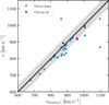 |
Fig. 2. Velocity measurements of PNe observed in the central field of M 105 compared to those observed in the field centred on NGC 3384 (blue) and the western e2PN.S field (red). The grey shaded region indicates the PN.S velocity error of 20 km s−1. |
We then matched the kinematic with the photometric catalogue, again using a matching radius of 5″. The unmasked region of overlap between the SuprimeCam and the PN.S fields of view spans 344.2 arcsec2 on the sky. Figure 3 shows the comparison of magnitudes measured from the [O III] image obtained with SuprimeCam and from the counter-dispersed images of the PN.S. The grey shaded region indicates where 99% of Subaru sources would fall if two independent measurements of their magnitudes mAB, Subaru were plotted against each other (see Appendix A.2 for details on the artificial star tests that we carried out). The typical PN.S magnitude errors (±0.2 mag, Douglas et al. 2007) are indicated by the error bar in the lower right corner of the figure. In the following section, we use the e2PN.S survey as an independent validation of the PN candidates detected with the SuprimeCam photometry.
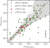 |
Fig. 3. Comparison of magnitudes of PNe measured with the Subaru SuprimeCam and the PN.S. The colour-coding is the same as in Fig. 1. The grey shaded region indicates where 99% of Subaru sources would fall if two independent measurements of their magnitudes mAB, Subaru were plotted against each other. The error bar in the lower right corner denotes the typical measurement error for magnitudes measured with the PN.S. |
2.5. Completeness and sources of contamination in the photometric catalogue
The evaluation of the completeness of our catalogue precedes any further quantitative analysis. We determined the spatial completeness of our SuprimeCam survey by calculating the recovery fraction of the synthetic PN population as a function of radius and the photometric completeness by calculating the recovery fraction as a function of magnitude (see Appendix A.5 for further details and Tables A.1 and A.2 for tabulated completeness values).
We furthermore needed to account for the presence of foreground and background contaminants. We estimated that 10% of the PNe candidates might be foreground objects such as faint Milky Way (MW) stars (see Appendix A.6.1). This is caused by the so-called spillover effect (Aguerri et al. 2005): due to photometric errors, continuum emitters such as faint foreground stars may end up with measured narrow-band fluxes that are brighter than their intrinsic flux and populate the CMD region from which PN candidates are selected. Background contaminants might be faint Ly-α galaxies at redshift z = 3.1 or [O II]3727 Å emitters at redshift z = 0.345, for whose presence we statistically account (see Appendix A.6.2 for details). We estimated their fraction to be 24.9 ± 5.0% of the completeness-corrected sample.
The PN.S does not cover the second bluer line of the [O III] doublet ([O III]4959 Å) that is commonly used to distinguish PNe from contaminants in spectroscopic follow-up surveys. It is, however, possible to use the PN.S data to exclude the majority of Ly-α galaxies that are associated with a continuum redder than the [O III]5007 Å emission line, as the continuum appears as a strike in slitless spectroscopy.
To estimate the contamination from Ly-α galaxies without a measurable continuum, we followed the argument presented by Spiniello et al. (2018): the number of background galaxies should be uniformly distributed in a velocity histogram. Figure 4 shows the LOS velocity distribution of PNe from the e2PN.S survey, with blue bands denoting the 1, 2, and 3σ intervals from the mean velocity of the sample. The LOS velocity distribution is composed of PNe that are associated with M 105 and NGC 3384, which results in a double-peaked asymmetric distribution. From the presence of two PNe in the velocity range 1500 − 2000 km s−1, beyond 3σ from the mean velocity, we expect eight PNe at most in the full velocity range (0 − 2000 km s−1). Therefore, we estimate the fraction of Ly-α contaminants without a measurable continuum to be 2.6% at most (8 of 307) in the e2PN.S survey.
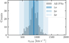 |
Fig. 4. Line-of-sight velocity distribution of PNe from the e2PN.S survey. The blue shaded regions denote the 1, 2, and 3σ intervals from the mean velocity (blue vertical line) of the sample. The double-peaked and asymmetric nature of the histogram is due to the fact that the survey covers NGC 3384 as well as M 105. |
We thus used the e2PN.S survey as an independent validation of the PN candidates detected based on SuprimeCam photometry. For this, we only considered the region of overlap of the two surveys, as illustrated in Fig. 5, and excluded the bright galaxy centres of M 105 and NGC 3384 (see Appendix A.1 for further details). The top panel of Fig. 6 shows the magnitude distribution of PN candidates and common objects between the two surveys in this region. The bottom panel of this figure shows the magnitude distribution of PN candidates without a counterpart in the e2 PN.S survey. Within the limiting magnitude of the shallowest e2PN.S field (m⋆ + 1), all but one PN candidate have a counterpart in the e2PN.S survey. Beyond this limit, the number of PNe candidates without a counterpart increases. We attribute this to two factors: (1) the larger depth of the SuprimeCam survey and (2) the presence of redshifted Ly-α emitters (black hatched histogram, see Appendix A.6.2 for details).
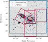 |
Fig. 5. Zoomed-in DSS image centred on M 105 with the PNe in the region of overlap between the SuprimeCam (blue rectangle) and e2 PN.S (red rectangles) surveys marked as blue and red crosses, respectively. The masked-out centres of NGC 3384 and M 105 are indicated by hatched ellipses. |
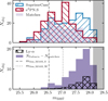 |
Fig. 6. Top: magnitude distribution of PN candidates from the SuprimeCam survey (hatched blue histogram) and PNe from the e2PN.S survey (hatched red histogram) in the region of overlap highlighted in Fig. 5. The magnitude distribution of objects identified in both surveys is shown in purple. The vertical lines denote the limiting magnitudes of the two shallowest e2PN.S fields, and the shaded grey region denotes magnitudes fainter than the limiting magnitude of the SuprimeCam survey. Bottom: magnitude distribution of PN candidates from the SuprimeCam survey with no counterpart in the e2PN.S (purple). The hatched histogram shows the expected distribution of background Ly-α galaxies at redshift z = 3.1 in the region of overlap scaled by the photometric completeness of the SuprimeCam survey. |
3. Stellar surface photometry of the Leo I group
In this section, we provide an overview of the stellar surface photometry of the two brightest galaxies in the field-of-view (FoV) of our PN surveys: M 105 and NGC 3384. This allows us to link the properties of the observed PNe to those of the underlying stellar populations in Sect. 4.
3.1. M 105
M 105 has been the target of numerous photometric studies: de Vaucouleurs (1948) first analytically described the light distribution of M 105, and it was one of the galaxies that were used to define the de Vaucouleurs law (see also de Vaucouleurs & Capaccioli 1979). In the following analyses, we used the relation determined by Capaccioli et al. (1990) based on B-band imaging to describe the surface brightness profile of M 105 analytically,
 (3)
(3)
where rM 105 is the major-axis radius measured from the centre of M 105 in units of arcseconds. Capaccioli et al. (1990) determined the effective radius to be  . They furthermore determined the mean ellipticity to be ϵM 105 = 0.111 ± 0.005 and the mean position angle to be
  . These parameters are summarised in Table 1 and the corresponding profiles as a function of radius are shown in Fig. 7a. Cappellari et al. (2007) determined a slightly smaller effective radius re = 42″ and ellipticity ϵ = 0.08 and a similar photometric position angle (PA = 67.9°) from HST/WFPC2 + MDM I-band images. The difference between the effective radii can likely be attributed to the different bands (I band versus B band) in which they were measured and the different limiting surface brightness values of the surveys.
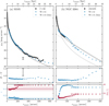 |
Fig. 7. Broad-band photometry of the galaxies M 105 (left) and NGC 3384 (right) in the Leo I group from Watkins et al. (2014, W+14). Top panel: B-band surface brightness profile, the middle panel shows the B − V colour profile, and the bottom panel shows the ellipticity (blue) and position angle (red), all as a function of major-axis radius. Open circles denote quantities measured from a binned image (9 pix × 9 pix). The error bar in the top left panel denotes the typical error on the B-band surface brightness, and the error bar the middle panel denotes typical measurement errors on the B − V colour for the binned data. Panel a: data from Capaccioli et al. (1990, black diamonds), and their best-fit de Vaucouleurs profile (grey line) in the top panel. Their mean ellipticity and position angle are indicated by shaded bands in the bottom panel. Panel b: colour-corrected 2MASS profile Skrutskie et al. (2006, black diamonds), and the corresponding disc-spheroid decomposition (dotted, dashed, and solid grey lines) by Cortesi et al. (2013b) are shown in the top panel. |
3.2. NGC 3384
For completeness, we also briefly discuss the photometric properties of the closest neighbouring galaxy of M 105, NGC 3384. Its isophotes overlap those of M 105. As NGC 3384 is an S0 galaxy viewed edge-on, its light can be decomposed into a contribution from its bulge (spheroid) and a contribution from its disc. Cortesi et al. (2013b) carried out a photometric disc-spheroid decomposition based on 2MASS K-band images (Skrutskie et al. 2006). They found that the spheroid light distribution is best described by a Sérsic profile,
 (4)
(4)
with Σe = 4.09 × 10⁻⁷, n = 4, κ = 7.67,  , ellipticity ϵspheroid = 0.17, and position angle
  . The disc light distribution is described by
 (5)
(5)
with Σd = 5.01 × 10⁻⁸,  , ϵdisc = 0.66, inclination i = 70°, and
  . These parameters are summarised in Table 1.
3.3. Holistic view from a deep, extended multi-band survey
As the photometric data described above have been taken at different telescopes and through different filters, their different photometric zero-points had to be taken into account before we were able to use them jointly. We therefore used deep wide-field B-band data, encompassing both galaxies, and resulting SB profiles from Watkins et al. (2014). We determined a colour correction of B − K = −3.75 for the profiles derived from the 2MASS data by Cortesi et al. (2013b). We furthermore determined a shift of −0.35 mag between the B-band profiles derived from Watkins et al. (2014) and Capaccioli et al. (1990) and corrected for it accordingly. The colour-corrected B-band SB profiles are shown in Fig. 7.
The deeper photometry of Watkins et al. (2014) revealed that the surface brightness profile of M 105 flattens at large radii with respect to the analytic de Vaucouleurs profile fit by Capaccioli et al. (1990). This flattening starts at approximately 750″. We discuss the implications of this observation further in Sect. 4.2.
4. Radial PN number density profile and the luminosity-specific PN number
The luminosity-specific PN number, α-parameter for short, relates a PN population with its parent stellar population. The α-parameter of a stellar population with NPN PNe and total bolometric luminosity Lbol is
 (6)
(6)
We refer to Buzzoni et al. (2006) for a theoretical investigation of the relation between the α-parameter and the age and metallicity of the underlying stellar population modelled through simple stellar populations (SSPs) and as a function of Hubble type.
4.1. Radial PN number density profile of M 105
In the following analyses, we only considered PNe candidates from the photometric catalogue from SuprimeCam narrow-band imaging; for this dataset, we could place robust estimates on the spatial and photometric completeness. Furthermore, to limit the contamination from PNe associated with the S0 galaxy NGC 3384, we only considered PNe that are geometrically uniquely associated with M 105. As illustrated in Fig. 8, we defined two dividing lines (shown in blue), both enclosing 110° from the negative major axis of M 105 and only considered PNe that lie west of these lines (selected PNe are highlighted in blue).
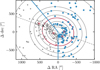 |
Fig. 8. On-sky PN distribution for the PN density and PNLF calculation in M 105. Only PNe from the imaging survey and to the right of the blue lines are considered (see text) to limit the contamination from NGC 3384 PNe. The PN density of M 105 is calculated in nine elliptical bins denoted in grey. The dashed line indicates the photometric major axis of M 105. The red contour corresponds to the vertical dashed line in Fig. 9. The black cross denotes the centre of NGC 3384. PNe within 0.5 mag from the PNLF bright cut-off at the distance of M 105 are marked with red crosses. North is up, and east is to the left. |
In total, 101 PN were selected for further analysis and were then binned into nine elliptical bins (grey ellipses in Fig. 8), whose geometry is defined by the isophotal parameters of M 105 as summarised in Table 1. The bin spacing was chosen such that each bin contained at least 12 PNe. In each bin, we determined the completeness-corrected number of PNe,
 (7)
(7)
where cs and cc denote the spatial and colour incompleteness, as detailed in Appendix A.5. The spatial completeness varies with radius and ranges from 77% to 98%, and the average colour completeness of our field is 87%.
The expected luminosity-averaged fraction of Ly-α emitters at redshift z = 3.1 is fLyα = 24.9 ± 5%, averaged over the SuprimeCam FoV (see Appendix A.6.2). The distribution of Ly-α contaminants can be approximated to be homogeneous in the SuprimeCam FoV. This implies that their contribution becomes stronger in the outer regime of low SB and low-PN number density. We therefore estimated the relative contribution of Ly-α emitters in each of the elliptical bins illustrated in Fig. 8: we randomly distributed the expected number of Ly-α emitters in the unmasked survey area and determined how many fell in each bin. We repeated this process 10 000 times to estimate error bars. The result is shown in the top panel of Fig. 9.
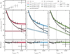 |
Fig. 9. Top panel: fractional contamination of the PN sample defined in Fig. 8 by Ly-α emitters in elliptical bins. The three panels of the middle row all show the same data: the grey crosses denote the PN number density calculated from the PN sample defined in Fig. 8 (101 PNe), which was shifted to the same scale as the B-band SB profile (grey stars; open symbols denote binned data, Watkins et al. 2014, W+14) and the bottom panels show the corresponding residuals. The vertical line denotes the transition from the inner PN-scarce to the outer PN-rich halo based on the change in the PN number density slope. Left column: the data are fit with a two-component SB profile (dark red line) consisting of a de Vaucouleurs-like inner component (dash-dotted grey line) and a constant outer component (dotted red line). The red line denotes the best-fit model to the PN number density. Middle column: the two-component SB profile (dark blue line) also has a de Vaucouleurs-like inner component (dash-dotted grey line), but the outer component is an exponential profile with scale height rh = 750″ (dotted blue line). The blue line denotes the best-fit model to the PN number density. Right column: the two-component SB profile (dark green line) has a de Vaucouleurs-like inner component (dash-dotted grey line) and an exponential component with scale height rh = 438″ (dotted green line). The green line denotes the best-fit model to the PN number density. The many thin lines are indicative of error ranges for the modelled profiles and were determined with Monte Carlo techniques (cf. Appendix B). |
The PN logarithmic number density profile is then
 (8)
(8)
where A(r) is the area of intersection of the elliptical annulus with the FOV of the observation, as illustrated in Fig. 8. From the offset μoff to the observed stellar SB profile, the α-parameter can be determined (see Sect. 4.2).
The PN number density profile shown in Fig. 9 was shifted to be on the same scale as the B-band surface brightness profile from Watkins et al. (2014). Within ∼438″(≈9re) from the centre of M 105, PN number density and stellar SB agree very well with each other, but beyond this transition radius, the PN number density profile significantly flattens with respect to the stellar SB profile. We note that the flattening occurs at 250″ shorter radial distance compared to the flattening of the SB profile that is observed beyond ∼750″. As already discussed in Longobardi et al. (2013, 2015b), we do not expect the flattening to be due to contaminants such as Ly-α-emitting galaxies because their contribution is statistically subtracted. The origin of the flattening of the PN number density is investigated in the following section.
4.2. Two-component photometric models for the extended halo of M 105
The flattening of the PN number density profile at large radii may be caused by a diffuse outer component. The second component, whether an additional component of the extended halo or in the form of diffuse IGL, is corroborated by the flattening of the stellar SB profile observed by Watkins et al. (2014). Such a flattening of the PN number density profile was also observed in the outer regions of other ETGs at the centres of groups and clusters of galaxies, such as M 87 in the Virgo cluster (Longobardi et al. 2013, 2015b, 2018) and M49 in the Virgo subcluster B (Hartke et al. 2017, 2018). It was attributed to intra-cluster light (ICL) or IGL with a distinct α-parameter value and spatial density distribution from the main halos of the galaxies.
To reproduce the flattening of the stellar SB profile at large radii, we constructed two sets of two-component photometric models, where the two components are denoted “inner” and “outer” according to the respective radial ranges in which they dominate the observed PN number density and SB profiles. In both sets of models, the stellar light distribution of the inner halo was modelled with a de Vaucouleurs profile as fitted by Capaccioli et al. (1990). We expressed it in terms of a Sérsic profile (Sérsic 1963),
 (9)
(9)
with
 (10)
(10)
Equation (9) is equivalent to Eq. (3) with a Sérsic index n = 4,  , and μe = 22.05 mag arcsec−2, after the colour correction determined in Sect. 3.3 is applied.
For the outer component, we considered two models:
-
A constant flat SB profile μouter(r) = μconst, which was also used by Longobardi et al. (2013) and Hartke et al. (2017) as part of their two-component models of the SB and PN number density profiles of galaxies in group and cluster environments.
-
An exponential profile defined as
 (11)
(11)where μ0 is its central surface brightness and rh its scale height, as used by Iodice et al. (2016), for example, to describe the extended halo of NGC 1399 at the core of the Fornax cluster.
The total SB of the two-component models is then given by
 (12)
(12)
In order to account for the discrepancy between the observed PN number density and stellar SB profiles at large radii (beyond 438″), we assumed that the two components have different α-parameters (Longobardi et al. 2013; Hartke et al. 2017):
 (13)
(13)
The two components Iinner, bol(r) and Iouter, bol(r) are the bolometric SB profiles weighted by the α-parameters of the respective populations, and s = 49.6 pc/″ is the conversion factor from angular to physical units for a distance of D = 10.3 Mpc.
The bolometric SB profiles Ibol(r) were obtained from the observed SB profiles μ(r):
 (14)
(14)
with the solar bolometric correction BC⊙ = −0.69, and K = 26.98 mag arcsec−2 is the B-band conversion factor to physical units L⊙ pc−2 (Buzzoni et al. 2006). While a fixed value of BCV = −0.85 with 10% accuracy can be assumed based on the study of stellar population models for different galaxy types, the bolometric correction in the B-band depends on galaxy colour (Buzzoni et al. 2006),
 (15)
(15)
Assuming a colour of B − V = 0.92 (cf. middle panel of Fig. 7a), we used a value of BCB = −1.76.
Instead of fitting αinner and αouter simultaneously, we first determined the well-constrained α-parameter of the inner component from the offset μoff between the PN number density and the inner stellar SB profile. Due to the large depth of our survey, we can directly determine the commonly used α2.5 parameter, which is calculated in a magnitude range from m⋆ to m⋆ + 2.5. In this magnitude range, we found the offset to the stellar SB profile to be μoff = 16.7 ± 0.1 mag arcsec−2. When the bolometric correction is applied as defined in Eq. (14), this offset translates into an α-parameter value of α2.5, inner = (1.17 ± 0.10) × 10−8
 .
.
Buzzoni et al. (2006) determined  based on the PN.S pointing centred on M 105. We scaled this value from α8 to α2.5 using the standard PNLF from Ciardullo et al. (1989), resulting in
  . This value is similar to the value determined in this work, but slightly higher. The difference may stem from a different treatment of the completeness corrections for the PN.S and SuprimeCam data.
We then proceeded to fit the outer SB profiles and corresponding α-parameters for the exponential and constant models using the non-linear least-squares minimisation routine LMFIT (Newville et al. 2014). We jointly minimised the residuals of the total stellar SB and PN number density profiles. In order to compare the models, we determined the Bayesian information criterion (BIC) as well as the reduced  for each of the best-fit models. Table 2 summarises the best-fit parameters, their error margins, and the goodness-of-fit parameters. For completeness, we also show the results of the fit of a single Sérsic profile to the data. We fixed the Sérsic index to n = 4 because otherwise, it was not possible to constrain the effective radius re and central surface brightness μeff. This model is ruled out due to its high BIC and reduced
  values compared to the two-component models discussed in the previous section.
Best-fit parameters for analytic models fit to the SB and PN number density.
For the first model, which has the constant outer SB profile, the best-fit parameters were μconst = 30.4 ± 0.1 and the ratio of the α-parameters α2.5, outer/α2.5, inner = 11.3 ± 4.8. The central and bottom left panels of Fig. 9 show the best-fit stellar SB (dark red) and PN number density profiles (red) in comparison to the data and their residuals. We drew 100 random samples for each free parameter from their posterior probability distribution to illustrate the error margins of the total model and its components (see Appendix B for a detailed description).
For the second model, which has an exponential outer SB profile, the free parameters were the central SB μ0, the ratio of the α-parameters α2.5, outer/α2.5, inner, and the scale height of the exponential profile rh. However, the latter proved to be very hard to constrain with the current data. We therefore decided to explore two models: one (Exponential 1) with a fixed rh = 750″, which is the major-axis transition radius at which the stellar SB profile deviates from a single de Vaucouleurs profile, and a second model (Exponential 2) with a fixed rh = 438″, which is the major-axis radius at which the PN number density profile deviates from the de Vaucouleurs profile. We thus only fit μ0 and α2.5, outer/α2.5, inner, whose best-fit values are summarised in Table 2. The resulting best-fit SB and PN number density profiles are shown in Fig. 9.
Based on the goodness of fit parameters BIC and  , the best-fit model has a constant outer SB profile because it has the lowest values. However, an outer component with constant SB and stars on radial orbits would not be compliant with the Jeans equations and a positive distribution function. With the current PN data, we cannot constrain the functional form of the component contributing to the stellar SB and PN number density profiles at large radii. As a next step, we used the constraints from the observed distribution of resolved MP and MR stellar populations in M 105, which we describe and address in the next section.
5. Constraints from resolved stellar populations
In order to explain the excess of PNe in the outer halos of early-type galaxies such as M 49 and M 87 in the Virgo cluster, Hartke et al. (2017, 2018) and Longobardi et al. (2015b, 2018) invoked the presence of an accreted MP population at large radii with a higher α-parameter value than that of the stellar population at the inner regions of these galaxies. In addition to the higher α-parameter value, further evidence for the presence of these MP stellar populations in the outer regions of M 49 and M 87 came from a change in PNLF slope at large radii, the gradients towards bluer colours, and from the kinematics of the PNe.
In the case of M 105, the direct evidence for an old halo population of MP stars comes from HST photometry (Harris et al. 2007a; Lee & Jang 2016). The grey hashed squares in Fig. 1 indicate the locations of the two HST pointings in the halo of M 105. In Figs. 10a and b, we show the integrated light profile (grey stars, Watkins et al. 2014), the PN number density (black crosses), and the total number density of RGB stars (grey squares), as well as the number density profiles of the MP (blue squares) and MR RGB stars (red squares) and the corresponding Sérsic profile fits (Lee & Jang 2016). As was emphasised by Harris et al. (2007a), we note that the number density of MP stars exceeds that of the MR stars at approximately ∼12 Reff, at a similar radius where the photometric SB profile deviates from a single Sérsic profile.
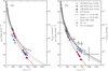 |
Fig. 10. a: comparison of the integrated B-band SB profiles (grey stars; open symbols denote binned data Watkins et al. 2014) with resolved stellar population studies of RGB stars (Lee & Jang 2016): grey squares indicate the number densities of all RGB stars, blue squares MP ([M/H] < 0.7) stars and red squares MR ([M/H] ≥ 0.7) stars. The coloured lines denote the best-fit Sérsic profiles to the respective stellar population determined by Lee & Jang (2016) with the best-fit indices stated in the legend of panel b. The RGB number densities were converted into SB using a constant conversion factor. b: same as panel a, but with a metallicity-weighted conversion factor from RGB number densities to SB (see Sect. 5.1) The right y-axis is only an indication of the RGB number density, as the conversion from μB is metallicity dependent. In addition, we also show the PN number density (black crosses). The solid black line represents the modelled PN number density profile, where the model consists of the MP and MR Sérsic profiles weighted by the respective α-parameter values. |
5.1. Comparing RGB number density and photometric SB profiles
In order to compare the number density profiles from RGB stars (Lee & Jang 2016) with the photometric SB profile (Watkins et al. 2014), Lee & Jang (2016) determined a constant conversion factor from the star counts in the inner HST field (200″ − 400″). However, using this constant conversion factor leads to a discrepancy between the modelled B-band SB at large radii and the SB measured by Watkins et al. (2014). Figure 10a shows that the measured photometric SB profile is brighter than the SB inferred from the RGB number counts. This discrepancy cannot be attributed to the measurement errors on the B-band SB, which are about ±0.25 mag for the binned data from Watkins et al. (2014). The origin must reside somewhere else: we hypothesise is that it is linked to the different contribution to the SB profile from the MR and MP stars as a function of radius.
A MP population of RGB stars is expected to yield a higher B-band luminosity than a MR population. We thus used the stellar population models from the MILES stellar library (Vazdekis et al. 2010) to estimate the luminosities emitted by the stellar populations with ages and metallicities that were determined for the MP and MR RGB stars by Lee & Jang (2016) in the different regions in M 105. We used BaSTi isochrones (Pietrinferni et al. 2013) and a Chabrier (2003) initial mass function. The ages of both populations were set to 12 Gyr. The peak of the metallicity distribution function (MDF) of the MR RGB stars is [M/H]≈0.0, and the peak metallicity of the MDF of the MP RGB stars is [M/H]≈ − 1.1 (Lee & Jang 2016, Fig. 7). The resulting scaling factors for the Sérsic profiles fit by Lee & Jang (2016) are then 1.42 for the MP profile and 0.81 for the MR profile. The corrected data points and Sérsic profiles are shown in Fig. 10b, which now agree better with the SB profile from Watkins et al. (2014).
5.2. Multi-component photometric models
Following the method presented in Sect. 4.2, we then explored whether the PN number density profile may be reproduced as the sum of the two Sérsic profiles previously fitted to the MP and MR RGB stars distribution by Lee & Jang (2016), allowing for a different α-parameter value for each population. The metallicity bins defined by Lee & Jang (2016) are [M/H] < −0.7 for the MP and [M/H] ≥ 0.7 for the MR RGB stars. We first calculated the α-parameter value for the inner halo, where the MR RGB stars dominate, and kept all the parameters of the Sérsic profile determined by Lee & Jang (2016) fixed. This resulted in  , which agrees well with the α-parameter value determined for the inner halo of M 105 in Sect. 4.2. We then determined the α-parameter value of the MP population by fitting the ratio αMR/αMP as shown in Fig. 10b. The fit to the PN number density results in αMR/αMP = 2.79 ± 0.91. However, the corresponding PN number density model is not a good representation of the measured PN number density profiles. It slightly overestimates the number of PNe in the inner halo and significantly underestimates the number of PNe at large radii. This is also reflected in the goodness-of-fit metrics reported in Table 3.
Best-fit parameters for analytic models fit to the SB and PN number density, with additional constraints from the RGB profiles from Lee & Jang (2016).
We then examined the MDFs in the two HST fields, and observed that while the RGB population with metallicity −1.0 ≤ [M/H] < −0.5 follows the Sérsic profile of the MR RGB population ([M/H] ≥ −0.5), the very MP RGB population with [M/H] < −1.0 fractionally increases the most in the outer halo. We therefore adopted the following alternative assumptions that
-
the intermediate metallicity (−1.0 ≤ [M/H] < −0.5) and MR RGB stars in the inner halo of M 105, that is, those in the south-eastern HST pointing, can be fitted by a single number density profile with slope n = 2.8 (as fitted fit to the MR stars in the inner and outer halo by Lee & Jang 2016, right panel of Fig. 8 therein), denoted by the blue dotted line in Fig. 11,
-
there is a distinct additional component of MP RGB stars ([M/H] < −1.0), which accounts for the higher fraction of MP stars at large radii, that is, in the western HST field.
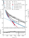 |
Fig. 11. Final stellar population decomposition of the integrated SB and PN number density profiles. Top panel: final best-fit model (black line) to the PN number density (black crosses). Comparison of the integrated B-band SB profiles (grey stars; open symbols denote binned data Watkins et al. 2014) with resolved stellar population studies of RGB stars (Lee & Jang 2016): blue triangles indicate MP stars, and red squares show MR stars. We used a metallicity-weighted conversion factor from RGB number densities to SB (see Sect. 5.1). The right y axis is thus only an indication of the RGB number density. The RGB number density profile is decomposed into an exponential MP profile (dashed blue line), an intermediate-metallicity (IM) Sérsic profile (dotted blue line), and the MR Sérsic (solid red line). The many thin grey lines are indicative of error ranges and were determined using Monte Carlo techniques (cf. Appendix B). Lower panel: residuals of the best fit. |
The MDFs fitted by Lee & Jang (2016, Table 4 therein), support these assessments. The MDF of the MP stars in the outer halo peaks at a metallicity that is 0.5 dex lower than the MDF in the inner halo, while the peak of the MDF of the MR stars only varies by 0.1 dex between the two bins. We quantified the excess of MP stars with respect to the intermediate-metallicity (dotted blue line in Fig. 11) and the MR component (continuous red line in Fig. 11) with an exponential profile that is denoted by the dashed blue line in Fig. 11. The exponential profile has a central surface brightness of μ0 = 27.7 ± 0.1 mag arcsec−2 and a scale radius of rh = 258 ± 2″.
We next confirmed whether the exponential profile correctly predicts the fraction of MP stars ([M/H] ≤ −1.0) in the inner HST pointing, that is, at a major-axis distance of ∼250″ from the centre of M 105. We used the Gaussian MDFs from Lee & Jang (2016, Table 4 therein), and determined that ∼18.6% of the 2040 stars in the MP component have metallicities [M/H] ≤ −1.0. This corresponds to ∼5% of the 7445 stars in the inner HST pointing. From the SB values of the exponential and total SB profiles defined above, 28.8 mag arcsec−2 and 25.7 mag arcsec−2, respectively, we expect ∼5.8% of the stars in the inner pointing to have metallicities [M/H] ≤ −1.0. We again applied a metallicity-dependent conversion factor from SB to RGB counts derived from stellar population models based on the MILES stellar library (see Sect. 5.1). The exponential profile thus correctly predicts the fraction of MP stars in the inner halo.
With this information at hand, we now proceed to calculate the α-parameter value associated with the MR and intermediate-metallicity RGB stars that dominate the number density profile in the inner halo. We assumed that the SB profile of this component is well modelled by the sum of the two Sérsic profiles with n = 2.8 described in the previous paragraph. We determined the α-parameter from the offset between the PN number density profile and the SB profile (using Eq. (8), see Sect. 4.1 for details). This resulted in  . This value agrees well with the value determined for the inner halo solely based on surface photometry (cf. Sect. 4).
To determine the α-parameter value associated with the MP RGB stars that dominate the number density profile in the outer halo, we constructed a two-component photometric model following the procedure outlined in Sect. 4.2. In this model, the inner component is the sum of the two Sérsic profiles describing the MR and intermediate-metallicity RGB stars, and the outer component is the exponential profile determined earlier in this section. As in Sect. 4.2, we did not fit the α-parameter directly, but instead fit the ratio α2.5, MP/α2.5, MR + IM, corresponding to  .
.
The thick black line in Fig. 11 indicates the final best-fit model to the PN number density. The goodness-of-fit parameters are reported in Table 3, and the posterior probability distribution of the model parameters is shown in Appendix B. The final model elegantly combines the information from integrated light (Watkins et al. 2014) resolved stellar populations (Harris et al. 2007a; Lee & Jang 2016) and PNe (this work) and provides a direct link between a high α-parameter value and the emergence of a MP halo that follows an exponential profile. The current finding for M 105 is significant for the study of PNe in the galaxy halos and the surrounding IGL because it provides the unambiguous direct evidence that a large luminosity-specific PN number value is linked to the presence of a MP ([M/H] < −1.0) RGB population.
6. Planetary nebula luminosity function of M 105
In addition to the PN number density profile, the PNLF is an important characteristic of a PN sample and can be used to make inferences about the properties of the underlying stellar population. The bright cut-off of the PNLF is an important secondary distance indicator. In this section, however, we focus on the variation of the faint-end PNLF slope, as there has been empirical evidence for a variation of PNLF slope with stellar population properties (Ciardullo et al. 2004; Ciardullo 2010; Longobardi et al. 2013, 2015b; Hartke et al. 2017, 2018). We therefore compared the observed PNLF to the generalised analytical formula introduced by Longobardi et al. (2013),
 (16)
(16)
In the equation above, c1 is a normalisation factor and c2 is the sought after faint-end slope. For c2 = 0.307, Eq. (16) takes the form of the standard PNLF introduced by Ciardullo et al. (1989).
We calculated the PNLF from the same sample that was used to determine the PN number density profile to limit contamination from PNe associated with NGC 3384 (see Fig. 8). The grey crosses in the left panel of Fig. 12 denote the luminosity function (LF) of the PN candidates. The observed LF is contaminated by Ly-α emitting galaxies at redshift z = 3.1 (see Appendix A.6.2). The estimated contribution of Ly-α emitters from Gronwall et al. (2007) is denoted by the red line and its expected 20% variation by the red shaded region. The observed number of PN candidates in our survey is larger than the estimated number of Ly-α contaminants in every magnitude bin. After statistically subtracting the estimated number of contaminants, we applied the colour- and detection-completeness corrections (Table A.2) and obtain the completeness-corrected (CC) PNLF shown with blue crosses in the left panel of Fig. 12. The crosses indicate the magnitude bin width and the expected errors due to counting statistics and the uncertainty of the Ly-α LF. For the brightest magnitude bin, the completeness-corrected number of PNe is smaller than one; we therefore only show an upper limit. The brightest PNe within 0.5 mag from the bright cut-off of M 105 are shown by red crosses in Fig. 8.
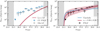 |
Fig. 12. PNLF in M 105. Left: observed LF of PN candidates (grey crosses) and PNLF of the completeness-corrected (CC) sample as defined in Fig. 8 (101 PNe) without accounting for contamination by Ly-α emitting background galaxies (blue crosses). Triangles denote upper limits. The solid red line shows the Ly-α LF and its variance due to density fluctuations indicated by the shaded regions (Gronwall et al. 2007). Right: PNLF of the completeness-corrected PN sample after statistical subtraction of the Ly-α LF (black crosses). Triangles denote upper limits. The solid blue curve denotes the standard Ciardullo PNLF with c2 = 0.307. The red line and shaded region denote our best-fit PNLF with c2 = 0.96 ± 0.30 In both panels, magnitudes fainter than the limiting magnitude and brighter than the bright cut-off are shaded in grey. |
In the right panel of Fig. 12, we again show the CC PNLF (black crosses) and different analytical PNLF models fit to the data. A standard Ciardullo PNLF with a fixed c2 = 0.307, as indicated by the solid blue line, is not a good representation of the data as it overestimates the number of bright PNe and underestimates the amount of faint PNe. We therefore fit the generalised PNLF as defined in Eq. (16) to the observed PNLF. Because the distance to M 105 is well determined from SBF measurements (D = 10.3 Mpc, Tonry et al. 2001), the only free parameters are the normalisation c1 and the faint-end slope, which we determine to be c2 = 0.96 ± 0.30. We used the non-linear least-squares minimisation method LMFIT (Newville et al. 2014) to fit to the completeness-corrected differential PNLF. The resulting analytic PNLF (denoted by the red line in the right panel of Fig. 12) reproduces the behaviour of the observed PNLF well. A PNLF with a steeper slope compared to M 31 (Ciardullo et al. 1989) is clearly favoured.
Motivated by the evidence of the changing PN populations in the inner and outer halo based on the PN number density profile and the inferred α-parameter values in Sect. 4, we investigated whether this difference also manifests itself in the PNLF morphology. We therefore divided our sample into two concentric elliptical bins and calculated the PNLF for each subsample individually. The dividing major-axis distance of 438″ is indicated as the red ellipse in Fig. 8 and by the dashed vertical line in Fig. 9.
The inner subsample is characterised by a density profile that decreases steeply with radius and contains 63 PNe. Its PNLF is shown in the left panel of Fig. 13. A fit of the generalised PNLF (solid red line and shaded region) results in a value of c2 = 0.51 ± 0.12, which is shallower than the slope of the total PN sample. The outer subsample is characterised by a flattened density profile and contains 38 PNe. Its PNLF is shown in the right panel of Fig. 13. A fit of the generalised PNLF (solid red line and shaded region) results in a slope of c2 = 1.42 ± 0.18, which is steeper than the slope of the total and inner PN samples.
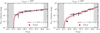 |
Fig. 13. Radial variation of the PNLF in M 105. Left: observed PNLF in the inner halo (black crosses) and best-fit generalised PNLF with c2 = 0.51 ± 0.12 (red line and shaded region). Right: observed PNLF in the outer halo (black crosses) and best-fit generalised PNLF with c2 = 1.42 ± 0.18 (red line and shaded region). |
The steeper PNLF in the outer subsample can be interpreted as an overabundance of faint PNe with respect to the inner subsample in the same magnitude bins, which may be the driving factor behind the flattening of the observed PN number density profile at large radii. Based on the information from the resolved stellar populations discussed in Sect. 5, we can closely link the change in the PNLF morphology with the higher number of old and MP stars in the outer halo observed by Harris et al. (2007a) and Lee & Jang (2016). While there is strong evidence for a stellar population mix in the outer halo of M 105, the PNLF beyond rmajor ≥ 438″ does not deviate from a single generalised exponential LF with a cut-off at M⋆. Rodríguez-González et al. (2015) fitted analytic two-mode PNLFs to PN populations in several nearby and Local Group galaxies, where a dip in the PNLF was observed that was several magnitudes fainter than the bright cut-off. Jacoby & De Marco (2002) argued that such dips could be interpreted as due to the existence of a population of PNe with faster central star evolution, for instance, for a younger stellar population. Similarly, Bhattacharya et al. (2019) observed an ubiquitous rise in the faint-end PNLF in M 31, whose steepness can be inversely correlated with recent star formation (Bhattacharya et al. 2020). A change in metallicity might have similar effects, but our data are not deep enough to explore them because PNLF dips have been observed to be at least two magnitudes fainter than the bright cut-off.
7. Discussion and conclusions
7.1. Old, MP, and PN-rich outer halo of M 105
In Sect. 4 we combined our study of individual tracers (PNe) with deep broad-band photometry from Watkins et al. (2014) and found a strong flattening of the PN number density profile with respect to the stellar SB profile at large radii (≳9.8re). This flattening can be well reproduced with a two-component photometric model that consists of a PN-poor inner halo with a de Vaucouleurs profile and a PN-rich exponential outer component. Relying solely on the information from surface photometry, we were unable to constrain the scale radius of the exponential profile.
We constrained the shape of the exponential profile using the information from resolved stellar populations. Harris et al. (2007a) and Lee & Jang (2016) published number-density profiles of MR and MP RGB stellar populations in the halo of M 105. We combined the information from these studies to infer that the density distribution of the most MP stars ([M/H] < −1.0) follows an exponential profile with a central surface brightness of μ0 = 27.7 ± 0.1 mag arcsec−2 and a scale radius of rh = 258 ± 2″ (Sect. 5).
Using the information from the RGB populations, we constructed a two-component photometric model, where the two components were weighted by their α-parameter values. In the PN-poor inner halo, the light distribution is dominated by intermediate-metallicity ( − 1.0 ≤ [M/H] < −0.5) and MR ([M/H] ≥ −0.5) stars, while in the PN-rich outer halo the MP stars dominate the light distribution. The α-parameter values of the two components are as follows:
-
 for the inner PN-poor component, and
 -
 for the outer PN-rich component.
We find a difference of a factor of seven in the α-parameter values of the inner versus outer components, implying that the luminosity-specific PN number of the stellar population that traces the old and MP halo at large radii is seven times higher.
We interpret the high α-parameter value and the steep faint-end PNLF slope as tell-tale signs of an additional old and MP stellar population whose contribution towards the overall light distribution increases at large radii. This interpretation is corroborated by the results of Harris et al. (2007a) and Lee & Jang (2016) based on resolved stellar populations. While in earlier works (Longobardi et al. 2013; Hartke et al. 2017) this association was made mostly by inference, we are now able to directly establish the link between the high α-parameter value, the steep PNLF slope, and the increase in the old and MP stellar population in the outer regions of M 105 (identified by Harris et al. 2007a).
The data of Harris et al. (2007a) clearly ruled out a single chemical evolution sequence for the entire halo stellar population and instead suggested a multi-stage evolutionary model. For the outer MP halo, two different scenarios were proposed: Harris et al. (2007a) argued that the MP halo was built up from pristine gas and that star-formation therein was truncated early, at the time of cosmological reionisation. In contrast, Lee & Jang (2016) proposed a formation dominated by dissipationless mergers and accretion. The scenario by Harris et al. (2007a) implies that the faint MP halo reached the current extension out to 40−50 kpc at high redshift, which is at odds with the observed slow growth of the stellar half-mass radius as a function of redshift (van der Wel et al. 2008). The scenario proposed by Lee & Jang (2016) is more consistent with the current two-phase formation model for elliptical galaxies.
Based on our current photometric PN survey in M 105, we cannot yet fully distinguish between these two scenarios. The high α-parameter value associated with the old and MP population is similar to the α-parameter values of Local Group dwarf irregular galaxies such as Leo I, Sextans A, and Sextans B, which lie between 3 × 10⁻⁸ and  (Buzzoni et al. 2006) and are in line with the accretion scenario proposed by Lee & Jang (2016). The new kinematics from the PN.S may provide viable information because we would be able to measure a higher velocity dispersion in the outer halo if it were accreted. Recent results on the outer halos of M 49 and M 87 (Hartke et al. 2018; Longobardi et al. 2018) definitely support the two-phase formation scenario.
7.2. Extended halo or IGL of the Leo I group?
The results from our PN photometry point towards an extended but rather faint outer stellar envelope that dominates the observed PN number density profile at large radii from the centre of M 105, which is one of the group-dominant galaxies in the Leo I group. The SB of the exponential outer component that we associate with these PNe falls below the detection limit of μB = 30 mag arcsec−2 of Watkins et al. (2014) beyond a distance of 750″. It is therefore not surprising that Watkins et al. (2014) concluded that there was no outer component in addition to the halo of M 105.
Based on the vastly different α-parameter value associated with the MP stellar populations and the distinct PNLF slope, we can already confirm a distinct origin of the stellar population associated with this outer exponential profile. Further independent evidence in support to the IGL classification of this component comes from the colour-magnitude diagram (CMD) of the resolved RGB stars in the western HST field (Harris et al. 2007a; Lee & Jang 2016): it has the same properties and MDF as the CMD and the corresponding MDF of the resolved intra-cluster RGB stars tracing the ICL in the Virgo core (Williams et al. 2007).
We can further identify common traits between the PN population and integrated-light properties at large radii in M 105 compared to other group- and cluster-dominant galaxies. As we discussed in the previous paragraphs, the strong increase in the α-parameter value at large radii and the exponential SB profile for the PN-rich component were also observed for the ICL/IGL surrounding cluster and group-dominant galaxies. For example, the exponential profile around M 105 has a quite similar scale length rh to that in M 49, see Spavone et al. (2017), while its central SB μ0 value is more than a magnitude fainter in M 105 than M 49. When the values of the structural parameters for the exponential component in M 105 are compared with those of the outer exponential components identified in more massive systems such as the BCGs NGC 3311 in the Hydra cluster (Arnaboldi et al. 2012) or NGC 1399 in the Fornax cluster (Iodice et al. 2016), the μ0 values increases by several magnitudes and the scale radius decreases by a factor two, signalling an increase in total luminosity and hence light fraction of the diffuse outer component with mass.
Returning to M 105, we can estimate the IGL fraction, assuming that the IGL is traced by the PNe and RGB stars associated with the exponential SB profile that we fit to the MP stars. We first estimated the bolometric luminosity of the diffuse exponential component. When we integrate the exponential profile over the total area of our SuprimeCam survey, we obtain Lbol, MP = 2.04 × 10⁹ L⊙. Within the limiting magnitude of our survey, we would hence expect 145 PNe to be associated with the exponential outer component. For comparison, the total bolometric luminosity associated with the main halo within our survey of M 105 is Lbol, MR + IM = 5.1 × 10¹⁰ L⊙. This luminosity would correspond to over 510 PNe, assuming an α-parameter value equal to α2.5, MR + IM as stated above. Because of incompleteness, especially in the bright galaxy centre, we observed significantly fewer PNe. We therefore determine the fraction of PNe associated with the outer component to be 22%. We note that this number is higher than that determined by Castro-Rodríguez et al. (2003) in the vicinity of the H I ring. The fraction of the bolometric luminosities of IGL versus the total light in galaxies is thus 3.8%, which is larger than the upper limit stated by Watkins et al. (2014). We note that the luminosity estimate of the diffuse component compares well with that of single ultra-diffuse galaxies (UDGs) observed in groups and clusters of galaxies (Mihos et al. 2015). UDGs are one viable progenitor of IGL stars: as a result of their low mass and density, they can be easily stripped, and their material can be deposited at large radii in the halo of a massive ETG (Amorisco 2017).
In Paper II of this series we will address the origin of the IGL by evaluating the dynamical status of the PNe populations at large radii based on the recently obtained kinematics in the framework of e2PN.S ETG survey. This will then also enable us to draw comparisons between the IGL/ICL kinematics in different environments and compare these results with recent integral-field spectroscopic surveys of massive ETGs (e.g. Ma et al. 2014). The assessment of the IGL in the Leo I group is particularly relevant because this group represents a benchmark for the IGL properties at the low-mass end of the galaxy group and cluster mass function.
7.3. Outlook
We have presented evidence that PNe trace a faint, MP component around M 105 in the Leo I group on the basis of deep photometry and number-count profiles of PNe and resolved stellar populations. Kluge et al. (2020) surveyed hundreds of brightest cluster galaxies (BCGs) at low redshift (z < 0.08) and fitted their SB profiles with double Sérsic models. They found a wide scatter between the transition radius of the two Sérsic profiles and the corresponding SB at this radius, which led them to the conclusion that the outer Sérsic profile probably does not trace the ICL. Even though we used a different functional decomposition, the conclusion of Kluge et al. (2020) might be applied to M 105 and its exponential outer component. Analyses of numerical simulations have shown that it is challenging to distinguish IGL or ICL components from outer envelopes that are gravitationally bound to the galaxy based on SB profiles alone (e.g. Cooper et al. 2015). In order to associate the diffuse component surrounding M 105 with the IGL, we need to know whether it is gravitationally bound to the group potential. This question cannot be answered based on photometric surveys alone.
In Paper II of this series, the analysis of the PN kinematics based on a photometric and kinematic decomposition of M 105 and NGC 3384 will be presented. These new data will provide first constraints on the physical state of the extended exponential outer component and the surrounding IGL identified here.
IRAF is distributed by the National Optical Astronomy Observatories, which are operated by the Association of Universities for Research in Astronomy, Inc., under cooperative agreement with the National Science Foundation.
Acknowledgments
The authors thank S. Okamura for his contribution towards the Subaru observations. We greatly acknowledge the support and advice of the ING and Subaru staff. We also thank A. E. Watkins and J. C. Mihos for the provision of the tabulated surface-brightness and colour profiles of M 105 and NGC 3384 and M. G. Lee and I. S. Jang for the provision of the density profiles of the resolved RGB stellar populations in the halo of M 105. We thank the organisers of the “Light in the suburbs” conference for the many stimulating discussions during the conference. JH thanks A. Agnello, I. Söldner-Rembold, and C. Spiniello for useful comments and discussions. JH and CP furthermore acknowledge support from the IMPRS on Astrophysics at the LMU Munich. We thank the referee Marc Sarzi for his constructive comments and the careful reading of the manuscript. This research made use of ASTROPY (Astropy Collaboration 2013), ASTROPLAN (Morris et al. 2018), ASTROQUERY (Ginsburg et al. 2019), ASTROMATIC-WRAPPER, CORNER (Foreman-Mackey 2016), EMCEE (Foreman-Mackey et al. 2013), LMFIT (Newville et al. 2014), MATPLOTLIB (Hunter 2007), NUMPY (Van Der Walt et al. 2011), and SYMPY (Meurer et al. 2017). This research has made use of the SIMBAD database, operated at CDS, Strasbourg, France (Wenger et al. 2000). This research has made use of the VizieR catalogue access tool, CDS, Strasbourg, France. The original description of the VizieR service was published in Ochsenbein et al. (2000). This publication has made use of data products from the Two Micron All Sky Survey, which is a joint project of the University of Massachusetts and the Infrared Processing and Analysis Center/California Institute of Technology, funded by the National Aeronautics and Space Administration and the National Science Foundation. The Digitized Sky Surveys were produced at the Space Telescope Science Institute under U.S. Government grant NAG W-2166. The images of these surveys are based on photographic data obtained using the Oschin Schmidt Telescope on Palomar Mountain and the UK Schmidt Telescope. The plates were processed into the present compressed digital form with the permission of these institutions. This research has made use of NASA’s Astrophysics Data System.
References
- Aguerri, J. A. L., Gerhard, O. E., Arnaboldi, M., et al. 2005, AJ, 129, 2585 [NASA ADS] [CrossRef] [Google Scholar]
- Amorisco, N. C. 2017, MNRAS, 464, 2882 [NASA ADS] [CrossRef] [Google Scholar]
- Arnaboldi, M., Aguerri, J. A. L., Napolitano, N. R., et al. 2002, AJ, 123, 760 [NASA ADS] [CrossRef] [Google Scholar]
- Arnaboldi, M., Freeman, K. C., Okamura, S., et al. 2003, AJ, 125, 514 [NASA ADS] [CrossRef] [Google Scholar]
- Arnaboldi, M., Ventimiglia, G., Iodice, E., Gerhard, O., & Coccato, L. 2012, A&A, 545, A37 [NASA ADS] [CrossRef] [EDP Sciences] [Google Scholar]
- Arnaboldi, M., Pulsoni, C., Gerhard, O., & PN.S Consortium 2017, IAU Symp., 323, 279 [NASA ADS] [Google Scholar]
- Astropy Collaboration (Robitaille, T. P., et al.) 2013, A&A, 558, A33 [NASA ADS] [CrossRef] [EDP Sciences] [Google Scholar]
- Belokurov, V., Evans, N. W., Irwin, M. J., et al. 2007, ApJ, 658, 337 [Google Scholar]
- Bertin, E. 2006, ASP Conf. Ser., 351, 112 [NASA ADS] [Google Scholar]
- Bertin, E., & Arnouts, S. 1996, A&AS, 117, 393 [NASA ADS] [CrossRef] [EDP Sciences] [Google Scholar]
- Bertin, E., Mellier, Y., Radovich, M., et al. 2002, ASP Conf. Ser., 281, 228 [Google Scholar]
- Bhattacharya, S., Arnaboldi, M., Hartke, J., et al. 2019, A&A, 624, A132 [NASA ADS] [CrossRef] [EDP Sciences] [Google Scholar]
- Bhattacharya, S., Arnaboldi, M., Gerhard, O., et al. 2020, A&A, submitted [Google Scholar]
- Bullock, J. S., & Johnston, K. V. 2005, ApJ, 635, 931 [NASA ADS] [CrossRef] [Google Scholar]
- Buzzoni, A., Arnaboldi, M., & Corradi, R. L. M. 2006, MNRAS, 368, 877 [NASA ADS] [CrossRef] [Google Scholar]
- Capaccioli, M., Held, E. V., Lorenz, H., & Vietri, M. 1990, AJ, 99, 1813 [NASA ADS] [CrossRef] [EDP Sciences] [Google Scholar]
- Cappellari, M., Emsellem, E., Bacon, R., et al. 2007, MNRAS, 379, 418 [NASA ADS] [CrossRef] [Google Scholar]
- Castro-Rodríguez, N., Aguerri, J. A. L., Arnaboldi, M., et al. 2003, A&A, 405, 803 [NASA ADS] [CrossRef] [EDP Sciences] [Google Scholar]
- Chabrier, G. 2003, PASP, 115, 763 [Google Scholar]
- Ciardullo, R. 2010, PASA, 27, 149 [NASA ADS] [Google Scholar]
- Ciardullo, R., Jacoby, G. H., Ford, H. C., & Neill, J. D. 1989, ApJ, 339, 53 [NASA ADS] [CrossRef] [Google Scholar]
- Ciardullo, R., Feldmeier, J. J., Jacoby, G. H., et al. 2002, ApJ, 577, 31 [NASA ADS] [CrossRef] [Google Scholar]
- Ciardullo, R., Durrell, P. R., Laychak, M. B., et al. 2004, ApJ, 614, 167 [Google Scholar]
- Ciardullo, R., Gronwall, C., Wolf, C., et al. 2012, ApJ, 744, 110 [NASA ADS] [CrossRef] [Google Scholar]
- Colless, M., Ellis, R. S., Taylor, K., & Hook, R. N. 1990, MNRAS, 244, 408 [NASA ADS] [Google Scholar]
- Cooper, A. P., Gao, L., Guo, Q., et al. 2015, MNRAS, 451, 2703 [NASA ADS] [CrossRef] [Google Scholar]
- Cortesi, A., Arnaboldi, M., Coccato, L., et al. 2013a, A&A, 549, A115 [NASA ADS] [CrossRef] [EDP Sciences] [Google Scholar]
- Cortesi, A., Merrifield, M. R., Coccato, L., et al. 2013b, MNRAS, 432, 1010 [NASA ADS] [CrossRef] [Google Scholar]
- Crnojević, D., Sand, D. J., Spekkens, K., et al. 2016, ApJ, 823, 19 [NASA ADS] [CrossRef] [Google Scholar]
- de Lorenzi, F., Gerhard, O., Coccato, L., et al. 2009, MNRAS, 395, 76 [NASA ADS] [CrossRef] [Google Scholar]
- de Vaucouleurs, G. 1948, Annales d’Astrophysique, 11, 247 [NASA ADS] [Google Scholar]
- de Vaucouleurs, G. 1975, Nearby Groups of Galaxies (Chicago, IL: University of Chicago Press), 557 [Google Scholar]
- de Vaucouleurs, G., & Capaccioli, M. 1979, ApJS, 40, 699 [NASA ADS] [CrossRef] [Google Scholar]
- Dekel, A., Stoehr, F., Mamon, G. A., et al. 2005, Nature, 437, 707 [NASA ADS] [CrossRef] [PubMed] [Google Scholar]
- Douglas, N. G., Arnaboldi, M., Freeman, K. C., et al. 2002, PASP, 114, 1234 [NASA ADS] [CrossRef] [Google Scholar]
- Douglas, N. G., Napolitano, N. R., Romanowsky, A. J., et al. 2007, ApJ, 664, 257 [NASA ADS] [CrossRef] [Google Scholar]
- Ferguson, A. M. N., Irwin, M. J., Ibata, R. A., Lewis, G. F., & Tanvir, N. R. 2002, AJ, 124, 1452 [NASA ADS] [CrossRef] [Google Scholar]
- Foreman-Mackey, D. 2016, J. Open Source Softw., 1, 24 [Google Scholar]
- Foreman-Mackey, D., Hogg, D. W., Lang, D., & Goodman, J. 2013, PASP, 125, 306 [CrossRef] [Google Scholar]
- Gawiser, E., Francke, H., Lai, K., et al. 2007, ApJ, 671, 278 [NASA ADS] [CrossRef] [Google Scholar]
- Ginsburg, A., Sipócz, B. M., Brasseur, C. E., et al. 2019, AJ, 157, 98 [NASA ADS] [CrossRef] [Google Scholar]
- Gronwall, C., Ciardullo, R., Hickey, T., et al. 2007, ApJ, 667, 79 [NASA ADS] [CrossRef] [Google Scholar]
- Hammer, F., Flores, H., Lilly, S. J., et al. 1997, ApJ, 481, 49 [CrossRef] [Google Scholar]
- Harris, W. E., Harris, G. L. H., Layden, A. C., & Wehner, E. M. H. 2007a, ApJ, 666, 903 [NASA ADS] [CrossRef] [Google Scholar]
- Harris, W. E., Harris, G. L. H., Layden, A. C., & Stetson, P. B. 2007b, AJ, 134, 43 [NASA ADS] [CrossRef] [Google Scholar]
- Hartke, J., Arnaboldi, M., Longobardi, A., et al. 2017, A&A, 603, A104 [NASA ADS] [CrossRef] [EDP Sciences] [Google Scholar]
- Hartke, J., Arnaboldi, M., Gerhard, O., et al. 2018, A&A, 616, A123 [NASA ADS] [CrossRef] [EDP Sciences] [Google Scholar]
- Helmi, A., Cooper, A. P., White, S. D. M., et al. 2011, ApJ, 733, L7 [NASA ADS] [CrossRef] [Google Scholar]
- Hogg, D. W., Cohen, J. G., Blandford, R., & Pahre, M. A. 1998, ApJ, 504, 622 [NASA ADS] [CrossRef] [Google Scholar]
- Hunter, J. D. 2007, Comput. Sci. Eng., 9, 90 [NASA ADS] [CrossRef] [Google Scholar]
- Iodice, E., Capaccioli, M., Grado, A., et al. 2016, ApJ, 820, 42 [NASA ADS] [CrossRef] [Google Scholar]
- Jacoby, G. H. 1989, ApJ, 339, 39 [NASA ADS] [CrossRef] [Google Scholar]
- Jacoby, G. H., & De Marco, O. 2002, AJ, 123, 269 [Google Scholar]
- Janowiecki, S., Mihos, J. C., Harding, P., et al. 2010, ApJ, 715, 972 [NASA ADS] [CrossRef] [Google Scholar]
- Kluge, M., Neureiter, B., Riffeser, A., et al. 2020, ApJS, 247, 43 [Google Scholar]
- Lee, M. G., & Jang, I. S. 2016, ApJ, 822, 70 [NASA ADS] [CrossRef] [Google Scholar]
- Longobardi, A., Arnaboldi, M., Gerhard, O., et al. 2013, A&A, 558, A42 [NASA ADS] [CrossRef] [EDP Sciences] [Google Scholar]
- Longobardi, A., Arnaboldi, M., Gerhard, O., & Mihos, J. C. 2015a, A&A, 579, L3 [NASA ADS] [CrossRef] [EDP Sciences] [Google Scholar]
- Longobardi, A., Arnaboldi, M., Gerhard, O., & Hanuschik, R. 2015b, A&A, 579, A135 [NASA ADS] [CrossRef] [EDP Sciences] [Google Scholar]
- Longobardi, A., Arnaboldi, M., Gerhard, O., Pulsoni, C., & Söldner-Rembold, I. 2018, A&A, 620, A111 [NASA ADS] [CrossRef] [EDP Sciences] [Google Scholar]
- Ma, C.-P., Greene, J. E., McConnell, N., et al. 2014, ApJ, 795, 158 [Google Scholar]
- Marmo, C., & Bertin, E. 2008, ASP Conf. Ser., 394, 619 [Google Scholar]
- Meurer, A., Smith, C. P., Paprocki, M., et al. 2017, PeerJ Comput. Sci., 3, e103 [CrossRef] [Google Scholar]
- Michel-Dansac, L., Duc, P.-A., Bournaud, F., et al. 2010, ApJ, 717, L143 [Google Scholar]
- Mihos, J. C., Harding, P., Feldmeier, J., & Morrison, H. 2005, ApJ, 631, L41 [NASA ADS] [CrossRef] [Google Scholar]
- Mihos, J. C., Durrell, P. R., Ferrarese, L., et al. 2015, ApJ, 809, L21 [NASA ADS] [CrossRef] [Google Scholar]
- Mihos, J. C., Harding, P., Feldmeier, J. J., et al. 2017, ApJ, 834, 16 [NASA ADS] [CrossRef] [Google Scholar]
- Miyazaki, S., Komiyama, Y., Sekiguchi, M., et al. 2002, PASJ, 54, 833 [NASA ADS] [CrossRef] [Google Scholar]
- Morris, B. M., Tollerud, E., Sipócz, B., et al. 2018, AJ, 155, 128 [NASA ADS] [CrossRef] [Google Scholar]
- Müller, O., Jerjen, H., & Binggeli, B. 2018, A&A, 615, A105 [NASA ADS] [CrossRef] [EDP Sciences] [Google Scholar]
- Newville, M., Stensitzki, T., Allen, D. B., & Ingargiola, A. 2014, https://doi.org/10.5281/zenodo.11813 [Google Scholar]
- Ochsenbein, F., Bauer, P., & Marcout, J. 2000, A&AS, 143, 23 [NASA ADS] [CrossRef] [EDP Sciences] [Google Scholar]
- Oser, L., Ostriker, J. P., Naab, T., Johansson, P. H., & Burkert, A. 2010, ApJ, 725, 2312 [NASA ADS] [CrossRef] [Google Scholar]
- Peebles, P. J. E. 1980, The Large-Scale Structure of the Universe (Princeton: Princeton University Press) [Google Scholar]
- Pierce, M. J., & Tully, R. B. 1985, AJ, 90, 450 [Google Scholar]
- Pietrinferni, A., Cassisi, S., Salaris, M., & Hidalgo, S. 2013, A&A, 558, A46 [NASA ADS] [CrossRef] [EDP Sciences] [Google Scholar]
- Pulsoni, C., Gerhard, O., Arnaboldi, M., et al. 2018, A&A, 618, A94 [NASA ADS] [CrossRef] [EDP Sciences] [Google Scholar]
- Richardson, J. C., Ferguson, A. M. N., Johnson, R. A., et al. 2008, AJ, 135, 1998 [NASA ADS] [CrossRef] [Google Scholar]
- Rodríguez-González, A., Hernández-Martínez, L., Esquivel, A., et al. 2015, A&A, 575, A1 [NASA ADS] [CrossRef] [EDP Sciences] [Google Scholar]
- Romanowsky, A. J., Douglas, N. G., Arnaboldi, M., et al. 2003, Science, 301, 1696 [NASA ADS] [CrossRef] [PubMed] [Google Scholar]
- Rood, H. J., & Williams, B. A. 1984, ApJ, 285, L5 [NASA ADS] [CrossRef] [Google Scholar]
- Rood, H. J., & Williams, B. A. 1985, ApJ, 288, 535 [Google Scholar]
- Rudick, C. S., Mihos, J. C., & McBride, C. 2006, ApJ, 648, 936 [NASA ADS] [CrossRef] [Google Scholar]
- Schechter, P. 1976, ApJ, 203, 297 [Google Scholar]
- Schneider, S. 1985, ApJ, 288, L33 [NASA ADS] [CrossRef] [Google Scholar]
- Schneider, S. E., Helou, G., Salpeter, E. E., & Terzian, Y. 1983, ApJ, 273, L1 [Google Scholar]
- Sérsic, J. L. 1963, Boletin de la Asociacion Argentina de Astronomia La Plata Argentina, 6, 41 [Google Scholar]
- Skrutskie, M. F., Cutri, R. M., Stiening, R., et al. 2006, AJ, 131, 1163 [NASA ADS] [CrossRef] [Google Scholar]
- Sommer-Larsen, J. 2006, MNRAS, 369, 958 [NASA ADS] [CrossRef] [Google Scholar]
- Spavone, M., Capaccioli, M., Napolitano, N. R., et al. 2017, A&A, 603, A38 [NASA ADS] [CrossRef] [EDP Sciences] [Google Scholar]
- Spiniello, C., Napolitano, N. R., Arnaboldi, M., et al. 2018, MNRAS, 477, 1880 [Google Scholar]
- Starkenburg, E., Helmi, A., Morrison, H. L., et al. 2009, ApJ, 698, 567 [NASA ADS] [CrossRef] [Google Scholar]
- Steinmetz, M., & Navarro, J. F. 2002, New Astron., 7, 155 [NASA ADS] [CrossRef] [Google Scholar]
- Teplitz, H. I., Malkan, M. A., Steidel, C. C., et al. 2000, ApJ, 542, 18 [NASA ADS] [CrossRef] [Google Scholar]
- Theuns, T., & Warren, S. J. 1997, MNRAS, 284, L11 [CrossRef] [Google Scholar]
- Thomas, J., Saglia, R. P., Bender, R., et al. 2005, MNRAS, 360, 1355 [NASA ADS] [CrossRef] [Google Scholar]
- Tonry, J. L., Dressler, A., Blakeslee, J. P., et al. 2001, ApJ, 546, 681 [NASA ADS] [CrossRef] [Google Scholar]
- Van Der Walt, S., Colbert, S. C., & Varoquaux, G. 2011, Comput. Sci. Eng., 13, 22 [CrossRef] [Google Scholar]
- van der Wel, A., Holden, B. P., Zirm, A. W., et al. 2008, ApJ, 688, 48 [NASA ADS] [CrossRef] [Google Scholar]
- Vazdekis, A., Sánchez-Blázquez, P., Falcón-Barroso, J., et al. 2010, MNRAS, 404, 1639 [NASA ADS] [Google Scholar]
- Watkins, A. E., Mihos, J. C., Harding, P., & Feldmeier, J. J. 2014, ApJ, 791, 38 [NASA ADS] [CrossRef] [Google Scholar]
- Weijmans, A.-M., Cappellari, M., Bacon, R., et al. 2009, MNRAS, 398, 561 [NASA ADS] [CrossRef] [Google Scholar]
- Wenger, M., Ochsenbein, F., Egret, D., et al. 2000, A&AS, 143, 9 [NASA ADS] [CrossRef] [EDP Sciences] [Google Scholar]
- White, S. D. M., & Frenk, C. S. 1991, ApJ, 379, 52 [NASA ADS] [CrossRef] [Google Scholar]
- White, S. D. M., & Rees, M. J. 1978, MNRAS, 183, 341 [NASA ADS] [CrossRef] [Google Scholar]
- Williams, B. F., Ciardullo, R., Durrell, P. R., et al. 2007, ApJ, 656, 756 [NASA ADS] [CrossRef] [Google Scholar]
- Zacharias, N., Finch, C. T., Girard, T. M., et al. 2012, VizieR Online Data Catalog: I/322A [Google Scholar]
Appendix A: Extraction of the photometric PN catalogue
We used Source Extractor (SExtractor, Bertin & Arnouts 1996) to detect objects, measure their photometric properties, and to calculate background maps of our mosaic on- and off-band images. We denote the measured narrow- and broad-band magnitudes with mn and mb, respectively. The extracted magnitudes are in the AB magnitude system.
SExtractor detected and analysed objects for which the flux value in at least nine adjacent pixels was higher than 1.1 × σrms on the on-band image. As we aimed to measure the colour mn − mb of each emission-line object, we chose an aperture radius of 13 pixels and subsequently extracted the broad-band magnitude mb on the off-band image in dual-image mode, that is, in the same aperture as in the on-band image. Following Theuns & Warren (1997), we assigned a magnitude of mb = 28.7 to [O III] emitters for which no V-band magnitude could be measured in the off-band image. This corresponds to the flux of an [O III] emitter at the limiting magnitude mn, lim observed through a broad-band V filter.
A.1. Catalogue pre-processing
To prevent false detections of PNe due to image artefacts, we masked the pixel columns affected by dithering as well as regions with a high background value (e.g. due to charge transfer or saturated stars). We calculated the rms-background maps of the on- and off-band images using SExtractor and masked all pixels with values higher than 1.5 times the median background. Furthermore, we masked the central regions of the three bright galaxies M 105, NGC 3384, and NGC 3398 due to high background counts from diffuse galaxy light (black ellipses in Fig. 5). The masked regions account for 2.3% of the total survey area, which results in an unmasked survey area that covers 0.2365 deg2.
A.2. Limiting magnitude and photometric error
We determined the limiting magnitude of our survey by populating the on-band image with a synthetic PN population and determining its recovery fraction as a function of magnitude. The simulated PNe have a Moffat-shaped PSF profile as measured on the image (see Sect. 2.1.1) and follow the standard PNLF (Ciardullo et al. 1989) scaled to the distance of M 105. The synthetic population was added to the on-band image using the IRAF task mkobjects. The limiting magnitude mlim is defined as the magnitude at which the recovery fraction of the simulated population falls below 50%. We determine a limiting magnitude of mlim, n = 25.6, which corresponds to mlim, 5007 = 28.1.
We also used the synthetic population to determine the error on the extracted magnitudes by determining the difference between the simulated magnitudes and those extracted using SExtractor. We estimate the photometric error to be one standard deviation about the mean in ten magnitude bins. The resulting error bands are shown in Fig. 3.
A.3. Object selection
PN candidates were selected based on their position on the CMD and their unresolved light distribution.
A.3.1. CMD selection
Figure A.1 shows the mn versus mn − mb CMD of all extracted sources in the M 105 Suprime Cam field. In order to limit the contamination by [O II]3727 Å emitters at redshift z = 0.345, we imposed a colour-selection criterion of mn − mb < −1. This corresponds to an observed equivalent width of EWobs > 110 Å (Teplitz et al. 2000). No [O II] emitters with EWobs > 110 Å have been observed to date (Colless et al. 1990; Hammer et al. 1997; Hogg et al. 1998). PNe candidates are thus objects that have a colour excess mn − mb and are brighter than the limiting magnitude mlim, n = 25.6.
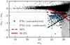 |
Fig. A.1. CMD for all sources (black dots) in the M 105 Suprime Cam field. Obects that lay below the grey horizontal line at mn − mb = −1 are emission-line objects with an equivalent width EWobs ≥ 110 Å. The magnitude range that is fainter than the limiting magnitude is denoted by the shaded grey region. The dashed (solid) red lines denote the 99.9% (99.9%) limits of the simulated foreground population. Black crosses denote the PNe candidates that were automatically selected, and blue dots denote those that were confirmed by visual inspection. |
Another source of possible contaminants are faint stellar sources (e.g. MW stars) that are scattered below the adopted colour excess because the increasingly large photometric errors are faint magnitudes. We therefore simulated a continuum population onto the on- and off-band images. The red dashed and solid lines in Fig. A.1 denote the 99% and 99.9% limits calculated from the extracted CMD of the simulated population. To limit the probability of including foreground stars to the 0.1% level, we only considered objects below the 99.9% limit for further analysis.
A.3.2. Point-like versus extended sources
At extragalactic distances, PNe appear as unresolved point-like sources. To limit contamination from extended sources (e.g. background galaxies or other objects with strong [O III] emission), we analysed the light distribution of the simulated PN population. We derived the following criteria for point-like sources:
-
The sources have half-light radii in the range 1 < Rh < 3.9 pix (top panels of Fig. A.2). This upper limit corresponds to 95% of the simulated population.
-
The sources lie above the 95% limit derived from the mn versus mn − mcore distribution of the simulated population (solid black line in the bottom panels of Fig. A.2). The core magnitude mcore is measured within a 5 pix aperture.
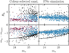 |
Fig. A.2. Point-source test for PN candidates in M 105. Left column: colour-selected PNe candidates. Right column: simulated PNe. Top row: half-light radius Rh as function of magnitude mn. Bottom row: mn − mcore as function of magnitude mn. In each panel, blue dots denote the PNe candidates selected based on their point-like appearance. Left column: red crosses denote cross-matches with the PN.S catalogue, which place additional constraints on the morphology of the selected PNe candidates from Subaru photometry. |
Sources that fulfil both criteria are denoted in blue in Fig. A.2 and as black crosses on the CMD in Fig. A.1. In contrast to Longobardi et al. (2013) and Hartke et al. (2017), we lifted the upper limit on the mn versus mn − mcore distribution (grey dashed line in Fig. A.2). This was motivated by the distribution of the PN.S-matched sources (red crosses) in the bottom left panel of Fig. A.2, the majority of which lie above the dashed grey line.
A.4. Catalogue validation and visual inspection
The automatically selected photometric catalogue was visually inspected, and any remaining spurious detections were removed, resulting in a final catalogue of 226 sources within the limiting magnitude of mlim, n = 25.6. These sources are highlighted with blue dots in the CMD in Fig. A.1. Their spatial distribution is shown in Fig. 1, superposed on the DSS image, in which they are denoted by blue crosses.
A.5. Catalogue completeness
Because PN-candidates were selected based on flux-ratio criteria, PNe that fell below the flux-threshold due to photometric errors would not have been detected. Table A.1 shows the spatial completeness of our survey within its limiting magnitude as a function of major-axis radius. The spatial completeness was calculated by determining the recovery fraction of the synthetic PN population simulated onto the unmasked regions of the on-band image. The spatial completeness is lowest in the innermost bin, which is due to the high background counts from the diffuse galaxy light of M 105.
Spatial completeness and unmasked survey area as function of major-axis radius.
The photometric completeness as a function of magnitude can be evaluated in terms of colour and detection completeness. The latter is simply the recovery fraction of the simulated population from the unmasked regions of the on-band image as a function of magnitude (cf. Appendix A.2). We determined the colour completeness by evaluating how many simulated PNe were scattered to CMD regions outside of the colour-selection criteria because of photometric errors as a function of magnitude. Both colour and detection completeness are tabulated in Table A.2.
Colour and detection completeness as function of magnitude.
A.6. Possible sources of contamination
A.6.1. Faint continuum objects
As we described earlier (cf. Appendix A.3), we limited our selection of objects to those that fall below the 99.9% line of a simulated continuum population to minimise the contamination by foreground objects such as faint MW stars. However, some of these objects will be scattered below this line. We estimated the fraction of foreground contaminants in the colour-selected sample by determining the total number of observed foreground stars down to mn, lim and assuming that 0.1% of these are scattered into the sample of colour-selected PNe. This results in 23 objects, which corresponds to a contribution of 10% of the extracted sample of 226 PNe.
A.6.2. Ly-α emitting background galaxies
Another source of contamination are faint background Ly-α galaxies that emit at the same wavelength as PNe in the Leo I group, if at redshift z = 3.1. To quantify this effect, we used the Ly-α LF determined by Gronwall et al. (2007), who carried out a deep survey for z = 3.1 Ly-α emission-line galaxies. The LF is characterised by a Schechter function (Schechter 1976). More recent surveys (e.g. Ciardullo et al. 2012) agree with this LF within 0.1 mag. The large-scale clustering of the Ly-α population at redshift z = 3.1 has a correlation length of r0 = 3.6 Mpc (Gawiser et al. 2007). At the distance of M 105, this corresponds to an angular scale of  , which is much larger than the SuprimeCam FoV. Within the limiting magnitude of our survey, we expect 56 Ly-α emitters, which corresponds to 24.9 ± 5.0% of the completeness-corrected sample. Figure 12 shows the corresponding LF. The contribution from [O II]3727 Å emitters at redshift z = 0.345 is already accounted for when the Gronwall et al. (2007) Ly-α LF is used (cf. Longobardi et al. 2013; Hartke et al. 2017).
Appendix B: Posterior probability distributions of the two-component model parameters
We calculated posterior probability distributions of the model parameters for each of the models presented in Sect. 4.2. We used the following logarithmic likelihood function (Foreman-Mackey et al. 2013):
![Mathematical equation: $$ \begin{aligned} \ln p(D|F_{\rm true}) = -\frac{1}{2}\sum _{n} \left[\frac{(g_{n}(F_{\rm true}) - D_{n})^2}{s_{n}^2}+\ln (2\pi s_{n}^2)\right], \end{aligned} $$](/articles/aa/full_html/2020/10/aa38009-20/aa38009-20-eq55.gif) (B.1)
(B.1)
where D is the data, that is, the observed stellar SB and PN number density profiles, F is the model parameters as detailed in Table 2, g is the model function (Eqs. (12) and (13)), and sn is the measurement uncertainties of the data. The resulting posterior probability distributions, calculated with the ensemble-based Monte Carlo Markov chain (MCMC) sampler EMCEE (Foreman-Mackey et al. 2013), are shown in Fig. B.1 for the model with the constant outer component, and Fig. B.2 shows the two models with an exponential outer component. Figure B.3 shows the posterior probability distribution for the final best-fit model with priors from resolved stellar populations. For each model, the posterior probability distribution was evaluated using 100 walkers and 5000 steps.
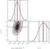 |
Fig. B.1. Posterior probability distribution of the parameters μconst and αouter/αinner of the two-component model with constant outer SB profile. The red lines denote the best-fit parameters determined in Sect. 4.2 (see Table 2), and the dashed lines show the 16%, 50%, and 84% levels. |
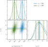 |
Fig. B.2. Posterior probability distribution of the parameters μconst and αouter/αinner of the two-component model with an exponential outer SB profile. The distribution shown in blue corresponds to a model with a fixed rh = 750″, and the distribution shown in green corresponds to a fixed rh = 438″. The solid lines denote the best-fit parameters determined in Sect. 4.2 (see Table 2), and the dashed lines show the 16%, 50%, and 84% levels. |
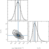 |
Fig. B.3. Posterior probability distribution of the parameters μoff and αouter/αinner of the two-component model with an exponential outer SB profile fit determined from the RGB number density profiles. The blue lines denote the best-fit parameters determined in Sect. 5 (see Table 3), and the dashed lines show the 16%, 50%, and 84% levels. |
All Tables
Best-fit parameters for analytic models fit to the SB and PN number density, with additional constraints from the RGB profiles from Lee & Jang (2016).
Spatial completeness and unmasked survey area as function of major-axis radius.
All Figures
|
Fig. 1. DSS image of M 105. Overplotted are the PN candidates from the Subaru survey (blue crosses), PNe from the ePN.S survey (Pulsoni et al. 2018, green pluses), and the e2PN.S survey (this work, red pluses and crosses). PNe in NGC 3384 from Cortesi et al. (2013a) are denoted with green circles. The red and green rectangles denote the ePN.S and e2PN.S fields, and the dashed blue rectangle indicates the SuprimeCam footprint. The grey hatched regions indicate the two HST fields analysed in Lee & Jang (2016). The scale bar in the lower right corner denotes 10 kpc. North is up, and east is to the left. |
| In the text | |
|
Fig. 2. Velocity measurements of PNe observed in the central field of M 105 compared to those observed in the field centred on NGC 3384 (blue) and the western e2PN.S field (red). The grey shaded region indicates the PN.S velocity error of 20 km s−1. |
| In the text | |
|
Fig. 3. Comparison of magnitudes of PNe measured with the Subaru SuprimeCam and the PN.S. The colour-coding is the same as in Fig. 1. The grey shaded region indicates where 99% of Subaru sources would fall if two independent measurements of their magnitudes mAB, Subaru were plotted against each other. The error bar in the lower right corner denotes the typical measurement error for magnitudes measured with the PN.S. |
| In the text | |
|
Fig. 4. Line-of-sight velocity distribution of PNe from the e2PN.S survey. The blue shaded regions denote the 1, 2, and 3σ intervals from the mean velocity (blue vertical line) of the sample. The double-peaked and asymmetric nature of the histogram is due to the fact that the survey covers NGC 3384 as well as M 105. |
| In the text | |
|
Fig. 5. Zoomed-in DSS image centred on M 105 with the PNe in the region of overlap between the SuprimeCam (blue rectangle) and e2 PN.S (red rectangles) surveys marked as blue and red crosses, respectively. The masked-out centres of NGC 3384 and M 105 are indicated by hatched ellipses. |
| In the text | |
|
Fig. 6. Top: magnitude distribution of PN candidates from the SuprimeCam survey (hatched blue histogram) and PNe from the e2PN.S survey (hatched red histogram) in the region of overlap highlighted in Fig. 5. The magnitude distribution of objects identified in both surveys is shown in purple. The vertical lines denote the limiting magnitudes of the two shallowest e2PN.S fields, and the shaded grey region denotes magnitudes fainter than the limiting magnitude of the SuprimeCam survey. Bottom: magnitude distribution of PN candidates from the SuprimeCam survey with no counterpart in the e2PN.S (purple). The hatched histogram shows the expected distribution of background Ly-α galaxies at redshift z = 3.1 in the region of overlap scaled by the photometric completeness of the SuprimeCam survey. |
| In the text | |
|
Fig. 7. Broad-band photometry of the galaxies M 105 (left) and NGC 3384 (right) in the Leo I group from Watkins et al. (2014, W+14). Top panel: B-band surface brightness profile, the middle panel shows the B − V colour profile, and the bottom panel shows the ellipticity (blue) and position angle (red), all as a function of major-axis radius. Open circles denote quantities measured from a binned image (9 pix × 9 pix). The error bar in the top left panel denotes the typical error on the B-band surface brightness, and the error bar the middle panel denotes typical measurement errors on the B − V colour for the binned data. Panel a: data from Capaccioli et al. (1990, black diamonds), and their best-fit de Vaucouleurs profile (grey line) in the top panel. Their mean ellipticity and position angle are indicated by shaded bands in the bottom panel. Panel b: colour-corrected 2MASS profile Skrutskie et al. (2006, black diamonds), and the corresponding disc-spheroid decomposition (dotted, dashed, and solid grey lines) by Cortesi et al. (2013b) are shown in the top panel. |
| In the text | |
|
Fig. 8. On-sky PN distribution for the PN density and PNLF calculation in M 105. Only PNe from the imaging survey and to the right of the blue lines are considered (see text) to limit the contamination from NGC 3384 PNe. The PN density of M 105 is calculated in nine elliptical bins denoted in grey. The dashed line indicates the photometric major axis of M 105. The red contour corresponds to the vertical dashed line in Fig. 9. The black cross denotes the centre of NGC 3384. PNe within 0.5 mag from the PNLF bright cut-off at the distance of M 105 are marked with red crosses. North is up, and east is to the left. |
| In the text | |
|
Fig. 9. Top panel: fractional contamination of the PN sample defined in Fig. 8 by Ly-α emitters in elliptical bins. The three panels of the middle row all show the same data: the grey crosses denote the PN number density calculated from the PN sample defined in Fig. 8 (101 PNe), which was shifted to the same scale as the B-band SB profile (grey stars; open symbols denote binned data, Watkins et al. 2014, W+14) and the bottom panels show the corresponding residuals. The vertical line denotes the transition from the inner PN-scarce to the outer PN-rich halo based on the change in the PN number density slope. Left column: the data are fit with a two-component SB profile (dark red line) consisting of a de Vaucouleurs-like inner component (dash-dotted grey line) and a constant outer component (dotted red line). The red line denotes the best-fit model to the PN number density. Middle column: the two-component SB profile (dark blue line) also has a de Vaucouleurs-like inner component (dash-dotted grey line), but the outer component is an exponential profile with scale height rh = 750″ (dotted blue line). The blue line denotes the best-fit model to the PN number density. Right column: the two-component SB profile (dark green line) has a de Vaucouleurs-like inner component (dash-dotted grey line) and an exponential component with scale height rh = 438″ (dotted green line). The green line denotes the best-fit model to the PN number density. The many thin lines are indicative of error ranges for the modelled profiles and were determined with Monte Carlo techniques (cf. Appendix B). |
| In the text | |
|
Fig. 10. a: comparison of the integrated B-band SB profiles (grey stars; open symbols denote binned data Watkins et al. 2014) with resolved stellar population studies of RGB stars (Lee & Jang 2016): grey squares indicate the number densities of all RGB stars, blue squares MP ([M/H] < 0.7) stars and red squares MR ([M/H] ≥ 0.7) stars. The coloured lines denote the best-fit Sérsic profiles to the respective stellar population determined by Lee & Jang (2016) with the best-fit indices stated in the legend of panel b. The RGB number densities were converted into SB using a constant conversion factor. b: same as panel a, but with a metallicity-weighted conversion factor from RGB number densities to SB (see Sect. 5.1) The right y-axis is only an indication of the RGB number density, as the conversion from μB is metallicity dependent. In addition, we also show the PN number density (black crosses). The solid black line represents the modelled PN number density profile, where the model consists of the MP and MR Sérsic profiles weighted by the respective α-parameter values. |
| In the text | |
|
Fig. 11. Final stellar population decomposition of the integrated SB and PN number density profiles. Top panel: final best-fit model (black line) to the PN number density (black crosses). Comparison of the integrated B-band SB profiles (grey stars; open symbols denote binned data Watkins et al. 2014) with resolved stellar population studies of RGB stars (Lee & Jang 2016): blue triangles indicate MP stars, and red squares show MR stars. We used a metallicity-weighted conversion factor from RGB number densities to SB (see Sect. 5.1). The right y axis is thus only an indication of the RGB number density. The RGB number density profile is decomposed into an exponential MP profile (dashed blue line), an intermediate-metallicity (IM) Sérsic profile (dotted blue line), and the MR Sérsic (solid red line). The many thin grey lines are indicative of error ranges and were determined using Monte Carlo techniques (cf. Appendix B). Lower panel: residuals of the best fit. |
| In the text | |
|
Fig. 12. PNLF in M 105. Left: observed LF of PN candidates (grey crosses) and PNLF of the completeness-corrected (CC) sample as defined in Fig. 8 (101 PNe) without accounting for contamination by Ly-α emitting background galaxies (blue crosses). Triangles denote upper limits. The solid red line shows the Ly-α LF and its variance due to density fluctuations indicated by the shaded regions (Gronwall et al. 2007). Right: PNLF of the completeness-corrected PN sample after statistical subtraction of the Ly-α LF (black crosses). Triangles denote upper limits. The solid blue curve denotes the standard Ciardullo PNLF with c2 = 0.307. The red line and shaded region denote our best-fit PNLF with c2 = 0.96 ± 0.30 In both panels, magnitudes fainter than the limiting magnitude and brighter than the bright cut-off are shaded in grey. |
| In the text | |
|
Fig. 13. Radial variation of the PNLF in M 105. Left: observed PNLF in the inner halo (black crosses) and best-fit generalised PNLF with c2 = 0.51 ± 0.12 (red line and shaded region). Right: observed PNLF in the outer halo (black crosses) and best-fit generalised PNLF with c2 = 1.42 ± 0.18 (red line and shaded region). |
| In the text | |
|
Fig. A.1. CMD for all sources (black dots) in the M 105 Suprime Cam field. Obects that lay below the grey horizontal line at mn − mb = −1 are emission-line objects with an equivalent width EWobs ≥ 110 Å. The magnitude range that is fainter than the limiting magnitude is denoted by the shaded grey region. The dashed (solid) red lines denote the 99.9% (99.9%) limits of the simulated foreground population. Black crosses denote the PNe candidates that were automatically selected, and blue dots denote those that were confirmed by visual inspection. |
| In the text | |
|
Fig. A.2. Point-source test for PN candidates in M 105. Left column: colour-selected PNe candidates. Right column: simulated PNe. Top row: half-light radius Rh as function of magnitude mn. Bottom row: mn − mcore as function of magnitude mn. In each panel, blue dots denote the PNe candidates selected based on their point-like appearance. Left column: red crosses denote cross-matches with the PN.S catalogue, which place additional constraints on the morphology of the selected PNe candidates from Subaru photometry. |
| In the text | |
|
Fig. B.1. Posterior probability distribution of the parameters μconst and αouter/αinner of the two-component model with constant outer SB profile. The red lines denote the best-fit parameters determined in Sect. 4.2 (see Table 2), and the dashed lines show the 16%, 50%, and 84% levels. |
| In the text | |
|
Fig. B.2. Posterior probability distribution of the parameters μconst and αouter/αinner of the two-component model with an exponential outer SB profile. The distribution shown in blue corresponds to a model with a fixed rh = 750″, and the distribution shown in green corresponds to a fixed rh = 438″. The solid lines denote the best-fit parameters determined in Sect. 4.2 (see Table 2), and the dashed lines show the 16%, 50%, and 84% levels. |
| In the text | |
|
Fig. B.3. Posterior probability distribution of the parameters μoff and αouter/αinner of the two-component model with an exponential outer SB profile fit determined from the RGB number density profiles. The blue lines denote the best-fit parameters determined in Sect. 5 (see Table 3), and the dashed lines show the 16%, 50%, and 84% levels. |
| In the text | |
Current usage metrics show cumulative count of Article Views (full-text article views including HTML views, PDF and ePub downloads, according to the available data) and Abstracts Views on Vision4Press platform.
Data correspond to usage on the plateform after 2015. The current usage metrics is available 48-96 hours after online publication and is updated daily on week days.
Initial download of the metrics may take a while.