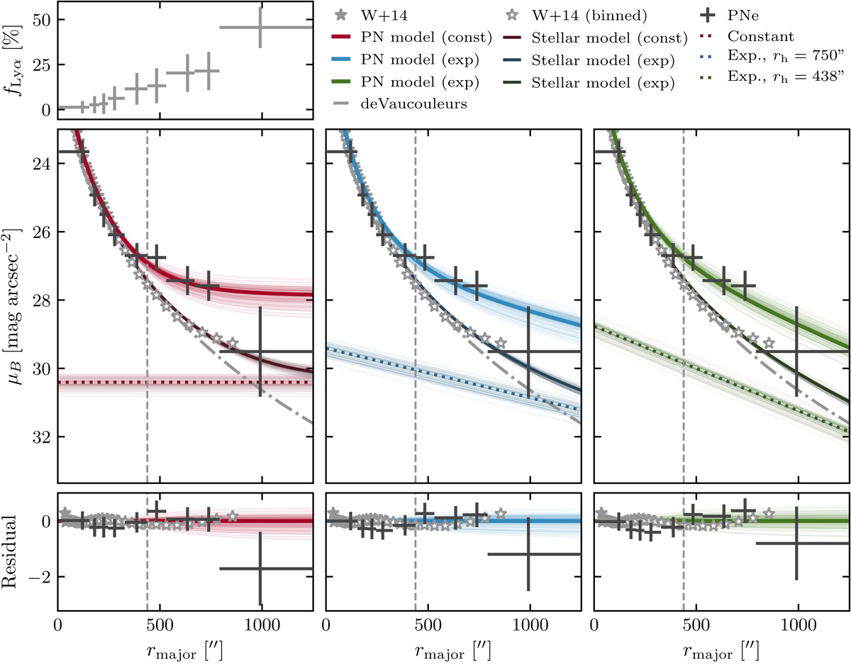
Top panel: fractional contamination of the PN sample defined in Fig. 8 by Ly-α emitters in elliptical bins. The three panels of the middle row all show the same data: the grey crosses denote the PN number density calculated from the PN sample defined in Fig. 8 (101 PNe), which was shifted to the same scale as the B-band SB profile (grey stars; open symbols denote binned data, Watkins et al. 2014, W+14) and the bottom panels show the corresponding residuals. The vertical line denotes the transition from the inner PN-scarce to the outer PN-rich halo based on the change in the PN number density slope. Left column: the data are fit with a two-component SB profile (dark red line) consisting of a de Vaucouleurs-like inner component (dash-dotted grey line) and a constant outer component (dotted red line). The red line denotes the best-fit model to the PN number density. Middle column: the two-component SB profile (dark blue line) also has a de Vaucouleurs-like inner component (dash-dotted grey line), but the outer component is an exponential profile with scale height r_h = 750″ (dotted blue line). The blue line denotes the best-fit model to the PN number density. Right column: the two-component SB profile (dark green line) has a de Vaucouleurs-like inner component (dash-dotted grey line) and an exponential component with scale height r_h = 438″ (dotted green line). The green line denotes the best-fit model to the PN number density. The many thin lines are indicative of error ranges for the modelled profiles and were determined with Monte Carlo techniques (cf. Appendix B).