| Issue |
A&A
Volume 641, September 2020
|
|
|---|---|---|
| Article Number | A22 | |
| Number of page(s) | 17 | |
| Section | Interstellar and circumstellar matter | |
| DOI | https://doi.org/10.1051/0004-6361/202038673 | |
| Published online | 01 September 2020 | |
Massive molecular gas reservoir around the central AGN in the CARLA J1103 + 3449 cluster at z = 1.44★
1
LERMA, Observatoire de Paris, PSL university, Sorbonne Université, CNRS, LERMA,
75014,
Paris, France
e-mail: This email address is being protected from spambots. You need JavaScript enabled to view it.
2
Université de Paris,
75013,
Paris, France
e-mail: This email address is being protected from spambots. You need JavaScript enabled to view it.
3
Jet Propulsion Laboratory, Cahill Center for Astronomy & Astrophysics, California Institute of Technology,
4800 Oak Grove Drive,
Pasadena,
CA, USA
4
Collège de France,
11 Place Marcelin Berthelot,
75231
Paris, France
5
Department of Astronomy, University of Geneva,
1205
Versoix, Switzerland
6
European Southern Observatory,
Karl-Schwarzschildstrasse 2,
85748
Garching, Germany
7
Cornell Center for Astrophysics and Planetary Science, Cornell University,
Ithaca,
NY
14853, USA
8
National Physical Laboratory,
Hampton Road,
Teddington,
Middlesex,
TW11 0LW, UK
9
Department of Astronomy, University of Florida,
Gainesville,
FL
32611-2055, USA
10
School of Physics and Astronomy, University of Nottingham, University Park,
Nottingham
NG7 2RD, UK
11
Department of Astronomy & Physics, Saint Mary’s University,
923 Robie Street,
Halifax,
NS
B3H 3C3, Canada
12
International Center for Radio Astronomy Research, Curtin University,
GPO Box U1987,
6102
Perth, Australia
13
Department of Physics, University of California,
One Shields Avenue,
Davis,
CA
95616, USA
Received:
16
June
2020
Accepted:
2
July
2020
Abstract
Passive early-type galaxies dominate cluster cores at z ≲ 1.5. At higher redshift, cluster core galaxies are observed to have on-going star-formation, which is fueled by cold molecular gas. We measured the molecular gas reservoir of the central region around the radio-loud active galactic nucleus (AGN) in the cluster CARLA J1103 + 3449 at z = 1.44 using NOEMA. The AGN synchrotron emission dominates the continuum emission at 94.48 GHz, and we measured its flux at the AGN position and at the position of two radio jets. Combining our measurements with published results over the range 4.71–94.5 GHz, and assuming Ssynch ∝ ν−α, we obtain a flat spectral index of α = 0.14 ± 0.03 for the AGN core emission, and a steeper index of α = 1.43 ± 0.04 and α = 1.15 ± 0.04 at positions close to the western and eastern lobes, respectively. The total spectral index is α = 0.92 ± 0.02 over the range 73.8 MHz–94.5 GHz. We detect two CO(2–1) emission lines, both blueshifted with respect to the AGN. Their emission corresponds to two regions, ~17 kpc southeast and ~14 kpc southwest of the AGN, not associated with galaxies. In these two regions, we find a total massive molecular gas reservoir of Mgastot = 3.9 ± 0.4 × 10¹⁰ M⊙, which dominates (≳60%) the central total molecular gas reservoir. These results can be explained by massive cool gas flows in the center of the cluster. The AGN early-type host is not yet quenched; its star formation rate is consistent with being on the main sequence of star-forming galaxies in the field (star formation rate ~30–140 M⊙ yr−1), and the cluster core molecular gas reservoir is expected to feed the AGN and the host star formation before quiescence. The other confirmed cluster members show star formation rates at ~2σ below the field main sequence at similar redshifts and do not have molecular gas masses larger than galaxies of similar stellar mass in the field.
Key words: galaxies: clusters: individual: CARLA J1103 + 3449 / galaxies: evolution / galaxies: star formation / galaxies: jets / radio continuum: galaxies
The reduced images and datacubes are only available at the CDS via anonymous ftp to cdsarc.u-strasbg.fr (130.79.128.5) or via http://cdsarc.u-strasbg.fr/viz-bin/cat/J/A+A/641/A22
© V. Markov et al. 2020
 Open Access article, published by EDP Sciences, under the terms of the Creative Commons Attribution License (http://creativecommons.org/licenses/by/4.0), which permits unrestricted use, distribution, and reproduction in any medium, provided the original work is properly cited.
1 Introduction
At redshifts z < 1.5 galaxy cluster cores are dominated by red, quenched, early-type galaxies, while blue, star-forming, late-type galaxies are mostly found in the field (e.g., Dressler 1980; Balogh et al. 1998, 2004; Postman et al. 2005; Mei et al. 2009; Rettura et al. 2011; Lemaux et al. 2012, 2019; Wagner et al. 2015; Tomczak et al. 2019). At higher redshifts, the results are somewhat conflicting, as it also becomes more difficult to define clusters of galaxies using measurements of their mass. Some results show that at z > 1.5 the star formation is already quenched in cluster cores (Kodama et al. 2007; Strazzullo et al. 2010; Papovich et al. 2010; Snyder et al. 2012; Grützbauch et al. 2012; Stanford et al. 2012; Zeimann et al. 2012; Gobat et al. 2013; Muzzin et al. 2013a; Newman et al. 2014; Mantz et al. 2014; Hayashi et al. 2017). Other observations show a reversal of the star formation–density relation and of ongoing star formation in cluster cores at z > 1.5, with a much more varied galaxy population compared to clusters at lower redshifts (Elbaz et al. 2007; Cooper et al. 2008; Tran et al. 2010; Brodwin et al. 2013; Santos et al. 2015; Mei et al. 2015; Alberts et al. 2016; Wang et al. 2016a; Noirot et al. 2016, 2018; Cucciati et al. 2018; Martinache et al. 2018; Shimakawa et al. 2018a,b; Tadaki et al. 2019). A reversal of the star formation at z ≳ 1 is also predicted from hydrodynamical and semi-analytical simulations (Tonnesen & Cen 2014; Chiang et al. 2017). Other cluster cores at z ≳ 1.5 present equal percentages of quiescent and star-forming galaxies (Fassbender et al. 2011; Tadaki et al. 2012; Zeimann et al. 2012; Mei et al. 2012; Noirot et al. 2016). A large presence of star-forming galaxies in cluster cores at z ~ 1.5–2 indicates that most of the star formation quenching observed at lower redshifts has not yet occurred, and that this is the key epoch of transformation of cluster galaxies from star forming to passive. At higher redshifts (z ~ 3–4), protoclusters show high star formation and star-burst activity (Umehata et al. 2015; Lewis et al. 2018; Miller et al. 2018; Oteo et al. 2018; Kubo et al. 2019; Hill et al. 2020; Ivison et al. 2020; Long et al. 2020; Toshikawa et al. 2020).
Galaxy star formation is fueled by cold and dense molecular gas (McKee & Ostriker 2007; Kennicutt & Evans 2012; Krumholz 2014). Therefore, galaxies rich in cold molecular gas are mostly star forming (bluish, mostly late-type spiral and irregular galaxies). Once the molecular gas is heated or stripped through different mechanisms, the star formation is quenched, and galaxiesstop forming new, young, blue stars, which explode relatively fast due to their short life cycle. These galaxies willslowly become dominated by long-lived red stars, and galaxies will evolve into red, mostly elliptical, quenched galaxies (Binney & Tremaine 1987; Kennicutt 1998; Kennicutt & Evans 2012). There are several possible processes that can be responsible for star formation quenching, and each plays a different role in cold molecular gas removal, at different epochs and with different timescales (Boselli & Gavazzi 2006). Quenching depends on both galaxy stellar mass and environment (Kauffmann et al. 2004; Baldry et al. 2006; Cucciati et al. 2010; Peng et al. 2010, 2012, 2014; Scoville et al. 2013; Darvish et al. 2015, 2016; Paccagnella et al. 2019). More massive galaxy stellar populations are quenched at earlier epochs (Thomas et al. 2005; Ilbert et al. 2013; Muzzin et al. 2013b; Tanaka et al. 2013; Guglielmo et al. 2015; Pacifici et al. 2016; Tomczak et al. 2016; Sklias et al. 2017; Davidzon et al. 2017; Morishita et al. 2019; Falkendal et al. 2019). Moreover, observations of galaxies of the same stellar mass at z < 1.5 show that the evolution from star forming to quiescent is more rapid for cluster galaxies than for their field counterparts (Raichoor et al. 2011; Muzzin et al. 2012; Papovich et al. 2012; Bassett et al. 2013; Shankar et al. 2013, 2014; Strazzullo et al. 2013; Scoville et al. 2013; Delaye et al. 2014; Guglielmo et al. 2015; Hatch et al. 2017; Tomczak et al. 2017; Foltz et al. 2018). This is due to additional environmental mechanisms, such as tidal stripping (Farouki & Shapiro 1981; Moore et al. 1999; Carleton et al. 2019), ram-pressure stripping (Abadi et al. 1999: McCarthy et al. 2008; Merluzzi et al. 2013; Jaffé et al. 2018), strangulation (Larson et al. 1980; Balogh & Morris 2000; Peng et al. 2012, 2015; Maier et al. 2016), and galaxy merging in the first epochs of cluster formation (Hopkins et al. 2006a; Dubois et al. 2016).
In the literature, the fraction of cold gas available for star formation is quantified as fgas = Mgas∕(M* + Mgas), or as a gas-to-stellar mass ratio Mgas∕M*. These quantities depend on redshift, galaxy stellar mass, and environment. Observations have shown that for galaxies at a given stellar mass, the gas fraction and gas-to-stellar mass ratio increase with redshift (Sargent et al. 2014; Genzel et al. 2015; Scoville et al. 2017; Silverman et al. 2018; Darvish et al. 2018; Tacconi et al. 2018). For galaxies at the same redshift, the gas fraction increases with decreasing stellar mass (Tacconi et al. 2013, 2018; Sargent et al. 2014; Lee et al. 2017). Finally, at z < 1.5, for galaxies of the same mass and at the same redshift, cluster galaxies show lower amounts of molecular gas and thus, lower gas fractions (Jablonka et al. 2013; Rudnick et al. 2017; Lee et al. 2017; Castignani et al. 2018; Hayashi et al. 2018). Some works have shown that at higher redshifts (z > 2), there is no difference in the gas fraction of cluster and field galaxies (Husband et al. 2016; Dannerbauer et al. 2017).
In order to assess the molecular gas mass, we can estimate the mass of the most dominant interstellar molecule – H2, which is also the star formation fuel. However, this molecule is practically invisible to observations due to its lack of a permanent dipole moment and the fact that its rotational dipole transitions require high temperatures, T > 100 K. In order to trace molecular hydrogen, rotational transitions of CO molecules are generally used for multiple reasons (Kennicutt & Evans 2012; Carilli & Walter 2013; Bolatto et al. 2013). The CO molecule has a weak permanent dipole moment and it is easily excited even inside cold molecular clouds due to its low energy rotational transitions (Kennicutt & Evans 2012; Bolatto et al. 2013). CO is also the second most abundant molecule after H2. CO rotational levels are excited by collisions with H2 molecules. Finally, CO rotational transitions lie in a relatively transparent millimeter window (Solomon & Vanden Bout 2005; Kennicutt & Evans 2012). The main drawback of tracing molecular gas with CO line emission is that CO is a poor tracer of the so-called CO-dark molecular gas, which usually accounts for a significant fraction (~ 30 to ~ 100%) of the total molecular gas mass in galaxies (Grenier et al. 2005; Wolfire et al. 2010; Abdo et al. 2010; Planck Collaboration XIX 2011; Pineda et al. 2013; Bisbas et al. 2017; Hall et al. 2020). In this paper, we focus on the molecular gas that can be detected by CO emission and molecular gas upper limits that can be inferred from the CO emission, with the caveat that this might not trace all the molecular gas in the galaxies that we study.
Few galaxy clusters are confirmed at z ≿ 1.5. Current observations of the CO emission line in clusters at these epochs show that cluster galaxies still have cold gas to fuel their star formation. However, these results are not yet statistically significant, and some results point toward higher molecular gas content in cluster galaxies with respect to the field and others to lower (Casasola et al. 2013; Rudnick et al. 2017; Noble et al. 2017; Hayashi et al. 2018; Coogan et al. 2018; Castignani et al. 2018). Molecular gas has also been detected in two protoclusters at z ~ 2.5 (Chapman et al. 2015; Wang et al. 2016b). Both protoclusters are dominated by star-forming (with a high starburst fraction), massive galaxies, with a substantial amount of molecular gas, and a small percentage of passive galaxies, which probably quenched after their accretion onto the cluster.
In this paper, we present IRAM (Institut de Radio Astronomie Millimetrique) NOEMA (NOrthern Extended Millimeter Array) observationsof the core of a confirmed cluster from the CARLA (Clusters Around Radio-Loud AGNs; Wylezalek et al. 2013) survey at z = 1.44, CARLA J1103 + 3449 (Noirot et al. 2018). CARLA J1103 + 3449 was selected as one of the highest CARLA IRAC color-selected overdensities (~ 6.5σ, from Wylezalek et al. 2014), and shows a ~ 3.5σ overdensity of spectroscopically confirmed sources (our Fig. 2, and Table 4 from Noirot et al. 2018). We found a large molecular gas reservoir south of the central AGN, consistent with gas inflows and outflows. We measured galaxy star formation rates and other properties for confirmed cluster members. We compared our results with similar observations in clusters and in the field.
Our observations, data reduction, and mapping are described in Sect. 2, the results are given in Sect. 3, the discussion is in Sect. 4, and finally, the summary of our results is given in Sect. 5. Throughout this paper, we adopt a ΛCDM cosmology, with of ΩM = 0.3, ΩΛ = 0.7, Ωk = 0, and h = 0.7, and assume a Chabrier initial mass function (IMF; Chabrier 2003).
2 Data
In this section, we describe the CARLA survey. Then, we present our observations and our available data.
2.1 CARLA survey
The CARLA survey (Wylezalek et al. 2013) is a substantial contribution to the field of high-redshift galaxy clusters at z > 1.5. CARLA is a 408h Warm Spitzer/IRAC survey of galaxy overdensities around 420 radio-loud AGN (RLAGN). The AGNs were selected across the full sky, approximately half radio loud quasars (RLQs) and half radio galaxies (HzRGs), and in the redshift range of 1.3 < z < 3.2. Wylezalek et al. (2013) identified galaxies at z > 1.3 around the AGNs in each field, using a color selection in IRAC channel 1 (λ = 3.6 μm; IRAC1, hereafter) and channel 2 (λ = 4.5 μm; IRAC2, hereafter). They found that 92% of the selected RLAGN reside in dense environments, with the majority (55%) of them being overdense at a > 2σ level, and 10% of them at a > 5σ level, with respect to the field surface density of sources in the Spitzer UKIRT Infrared Deep Sky Survey Ultra Deep Survey (SpUDS; Galametz et al. 2013), selected in the same way.
A Hubble Space Telescope Wide Field Camera 3 (HST/WFC3) follow-up of the twenty highest CARLA Spitzer overdensities (consisting of ten HzRGs and ten RLQs) spectroscopically confirmed sixteen of these at 1.4 <z < 2.8, and also discovered and spectroscopically confirmed seven serendipitous structures at 0.9 <z < 2.1 (Noirot et al. 2018). The structure members were confirmed as line emitters (in Hα, Hβ, [O II], and/or [O III], depending on the redshift) and have star formation estimates from the line fluxes (Noirot et al. 2018). The star formation of galaxies with a stellar mass ≳1010M⊙ is below the star-forming main sequence (MS) of field galaxies at similar redshift, and star-forming galaxies are mostly found within the central regions (Noirot et al. 2018). This program also provided WFC3 imaging in the F140W filter (WFC3/F140W) from which we obtained point-spread-function (PSF)-matched photometric catalogs (Amodeo et al., in prep.), and galaxy visual morphologies (Mei et al., in prep.).
From their IRAC luminosity function, Wylezalek et al. (2014) showed that CARLA overdensity galaxies have probably quenched faster and earlier compared to field galaxies. Some of the CARLA northern overdensities were also observed in either deep z-band or deep i-band, with the Gemini Multi-Object Spectrographs (GMOS) at the Gemini telescope (hereafter Gemini/GMOS), ISAAC at the European Southern Observatory Very Large Telescope (VLT/ISAAC) and ACAM at the WHT (William Herschel Telescope) telescope (WHT/ACAM). This permitted us to estimate their galaxy star formation rate histories, and we deduced that, on average, the star formation of galaxies in these targets had been rapidly quenched, producing the observed colors and luminosities (Cooke et al. 2015).
2.2 Optical and near-infrared multi-wavelength observations of CARLA J1103 + 3449
As a target of the Spitzer CARLA survey, CARLA J1103 + 3449 was observed with Spitzer IRAC1 and IRAC2 (Cycle 7 and 8 snapshot program; PI: D. Stern), for a total exposure of 800 s and 2000 s, respectively. The IRAC cameras have 256 × 256 InSb detector arrays with a pixel size of 1.22 arcsec and a field of view of 5.2 × 5.2 arcmin. Wylezalek et al. (2013) performed the data calibration and mapping with the MOPEX package (Makovoz & Khan 2005) and detected sources with SExtractor (Bertin & Arnouts 1996), using the IRAC-optimized SExtractor parameters from the work of Lacy et al. (2005). The final Spitzer IRAC1 and IRAC2 mosaic has a pixel size of 0.61 arcsec, after taking into account dithering and sub-pixelation.
The HST/WFC3 imaging and grism spectroscopy were obtained with a dedicated HST follow-up program (Program ID: 13 740; PI: D. Stern). We obtained F140W imaging (with a field of view of 2 × 2.3 arcmin2 at a resolution of 0.06 arsec pix−1, obtained after taking into account dithering), and G141 grism spectroscopy (with a throughput >10% in the wavelength range of 1.08 m < λ < 1.70 m and a spectral resolution of R = λ∕Δλ = 130). This grism was chosen in order to permit the identification of strong emission lines at our target redshift, such as Hα, Hβ, [O II], and [O III]. Noirot et al. (2016, 2018) performed the data reduction using the aXe (Kümmel et al. 2009) pipeline, by combining the individual exposures, and removing cosmic ray and sky signal. Noirot et al. (2018) performed the source detection with SExtractor (Bertin & Arnouts 1996) and extracted 2D spectra for each field, based on the positions and sizes of the sources. The redshifts and emission line fluxes were determined using the python version of mpfit and are published in Noirot et al. (2018).
CARLA J1103 + 3449 was followed-up with i-band imaging using WHT/ACAM (PI: N. Hatch; Cooke et al. 2015), and we obtained a PSF-matched photometric catalog in the WHT/ACAM i-band, WFC3/F140W (detection image), IRAC1, and IRAC2. The i-band, WFC3/F140W, and IRAC1 filters correspond to the UVJ rest-frame bandpasses at the redshift of CARLA J1103 + 3449. More details on the Spitzer IRAC, HST/WFC3, and WHT/ACAM observations, data reduction, and results can be found in Wylezalek et al. (2013, 2014), Noirot et al. (2016, 2018), and Cooke et al. (2015), respectively.
From a morphological (from the HST/F140W images) and photometric analysis of the central sources (Amodeo et al., in prep.; Mei et al., in prep.), the host galaxy of the AGN is an elliptical galaxy. The spiral galaxy close to the AGN is a spectroscopically confirmed member (Noirot et al. 2018), but is not detected as an independent galaxy in the IRAC images because of their poor spatial resolution. The bright central source south of the AGN is a star, with a spectral energy distribution consistent with a black body and not consistent with an early-type galaxy (ETG) spectrum.
2.3 Keck AGN spectrum observations
The redshift for the radio source B2 1100 + 35, associated with WISE J110326.19 + 344947.2 at the center of CARLA J1103 + 3449, was first reported in Eales et al. (1997) as z = 1.44, but with no spectrum presented. With no spectrum available from the Sloan Digital Sky Survey of the faint, red (g = 23.9 mag, i = 21.4 mag) optical counterpart to the radio source, we observed B2 1100 + 35 with the dual-beam Low Resolution Imaging Spectrometer (LRIS; Oke et al. 1995) at the Keck Observatory on UT 10 March 2019. The night suffered strongly from variable, often thick cloud cover.
The data were obtained through the 1.′′0 slit with the 5600 Å dichroic. The blue arm of the spectrograph used the 600 ℓ mm−1 grism (λblaze = 400 Å; resolving power R ≡ λ∕Δλ ~ 1600 for objects filling the slit), while the red arm used the 4000 ℓ mm−1 grating (λblaze = 8500 Å; R ~ 1300). Three 600 s exposures were attempted, though ultimately only one proved useful. We processed the spectrum using standard techniques, and flux calibrated the spectrum using observations of the standard stars Hilter 600 and HZ44 from Massey & Gronwall (1990) obtained the same night with the same instrument configuration. Figure 1 presents the processed spectrum. Multiple redshifted emission lines are detected, including broadened C IV λ1549 Å, narrow C III] λ1909 Å, narrow [Ne V] λ3426 Å, and strong, narrow [O II] λ3727 Å. Based on the latter feature, we report a redshift of z = 1.4427 ± 0.0005, where the uncertainty reflects both statistical uncertainties in the line fitting, as well as an estimate of systematic uncertainties in the wavelength calibration, and a comparison with other well-detected emission lines in this source. This measurement is consistent with the Noirot et al. (2018) AGN redshift measurement of z = 1.444 ± 0.006, from the HST/WFC3 grism observations (see above).
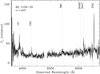 |
Fig. 1 Keck/LRIS spectrum of B2 1100 + 35, the radio galaxy at the center of CARLA J1103 + 3449. Since the night was not photometric, the y-axis only provides relative flux calibration. |
2.4 IRAM observations
For this work, we observe CARLA J1103 + 3449 with the IRAM/NOEMA (PI: A. Galametz, S. Mei), with eight antennas over a five-day period (28–30 Jul., 3–4 Aug. 2017), for a total exposure time of ~ 29 h (including overheads). The weather conditions were within the average precipitable water vapor (PWV ~10–20 mm). The average system temperaturewas Tsys ~ 100–200 K, and reached maximum values of 300 K. The sources used as RF (receiver bandpass) calibrator, the flux calibrator, and amplitude/phase calibrators were the 3C84 radio galaxy, the LKHA101 radio star, and the 1128 + 385 quasar, except on the 30 Jul., when we used the quasars 3C273, 1128 + 385 (measured on the 28 Jul.) and 1156 + 295.
We targeted the CO(2–1) emission line at the rest-frame frequency νrest = 230.538 GHz, which is redshifted to νobs = 94.48 GHz at z = 1.44 (approximately the mean confirmed cluster member redshift from Noirot et al. 2018), observed in the NOEMA 3 mm band. We covered our target with three pointings to map the AGN and the central cluster region. The pointings were positioned so that we could cover as many IRAC color-selected members as possible (~ 40) along with the seven (out of eight) HST/WFC3 spectroscopically confirmed members (green circles and a red star, for the AGN, in Fig. 2, based on Noirot et al. 2018). We chose the antenna configuration C to be able to separate cluster members in the cluster core. The beam size is 4.14 × 3.46 arcsec2, the PA = −171.01°, and the velocity resolution is 50 km s−1 (smoothed to 100 km s−1; see below).
We performed the entire NOEMA data calibration by running the pipeline in the clic package of the IRAM/GILDAS software1. We flagged additional data, modified antenna positions, and calibrated the flux again. While the pointing and the focus were excellent, the amplitude, and phase were of average quality because of the weather conditions.
With the reduced data, we created a CO(2–1) continuum emission mosaic map, by using the mapping package of the GILDAS software (Fig. 3, left). The map was obtained by averaging the flux over a velocity range of 2450 km s−1, excluding emission lines, with a background root mean square (rms) noise level of σ ~ 0.2 mJy beam−1. Then, we subtracted the continuum from the CO(2–1) emission in the uv-data set in order to obtain a clean, continuum-subtracted CO(2–1) map.
We calculated the rms noise level in the three pointing intersection regions of the CO(2–1) map (see Fig. 2). In this region, the original velocity resolution is 50 km s−1 and the rms noise level is σ ~ 0.8 × mJy beam−1. In order to improve the signal-to-noise ratio (S/N), we smoothed the CO(2–1) map to a final velocity resolution of 100 km s−1 by averaging two consecutive channels, and obtained a rms noise level of σ ~ 0.5 × mJy beam−1 after smoothing. We created the CO(2–1) intensity map by averaging the flux over a velocity range of 1200 km s−1 with the background rms noise level of σ ~ 0.2 mJy beam−1, and applied a primary beam correction (Fig. 3, right). On the mosaic edges, the rms noise level approximately doubles.
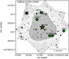 |
Fig. 2 Distribution of spectroscopically confirmed members of CARLA J1103 + 3449 (green circles) with the central AGN (red star) (Noirot et al. 2018). The background images are the two orientation HST/WFC3 F140W frames. The shaded area indicates the NOEMA mosaic map area. |
3 Results
In this section, we describe our results. First, we present the active galactic nucleus continuum emission. Then, we derive the molecular gas content in the cluster central region using CO(1-2) emission flux measurements.
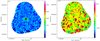 |
Fig. 3 Left: continuum emission map of the CARLA J1103 + 3449 cluster at 94.48 GHz. The map was obtained by averaging the flux over a velocity range of 2450 km s−1, outside of the emission lines. The rms noise level is σ ~ 0.2 mJy beam−1 in the central pointing intersection region, and the contours show the 3σ, 6σ, 9σ, etc. levels upto 24σ. Right: continuum subtracted CO(2–1) line emission mosaic map. The color wedge of the intensity maps is in Jy beam−1. The map was obtained by averaging the flux over a velocity range of 1200 km s−1, and has an average rms noise level of σ ~ 0.2 mJy beam−1 in the central pointing intersection region. The continuous lines show positive σ contours andthe dotted lines show negative σ contours. The contours show the 1σ, 2σ, and 3σ levels. The cross marks the phase center of the mosaic. The noise approximately doubles toward the map edges because of the primary beam correction. Both maps show an extended source in the cluster center. |
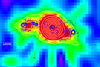 |
Fig. 4 Zoom-in on the continuum emission map of the extended source in the cluster center. The continuum emission contours (white) run as 3σ, 6σ, 9σ, etc. up to 24σ. The radio emission contours at 4.71 GHz from the work of Best et al. (1999) are overlaid on the image (in blue). The brightest continuum emission peak and one of the radio peaks are both centered on the AGN. The continuum emissions visually correspond to the position of the radio jets, suggesting the same or a connected physical origin. North is up and east is to the left. |
3.1 Active galactic nucleus continuum emission
On the continuum emission map at the observed frequency of νobs= 94.48 GHz, we detect an extended source in the cluster central region, with the brightest peak at the position of the AGN (>26σ, Fig. 4, white contours). Comparing the NOEMA continuum emission with radio observations at 4.71 GHz from Best et al. (1999) (Fig. 4, blue contours), the NOEMA continuum emission visually corresponds to the radio jets. Both the NOEMA extended continuum emission peak, and the central radio emission, correspond to the AGN position. We also detect significant (>6σ) continuum emission at the position of the tip of the eastern radio lobe (Fig. 4).
The position and the scale of this continuum emission detection follow the emission from the radio lobes, with the brighter and the fainter continuum components corresponding to the western and eastern radio lobe, respectively. This is consistent with the same or a connected physical origin of the two emissions. In fact, the AGN synchrotron emission dominates at both our NOEMA observed frequency (rest-frame ν ~ 230 GHz/λ ~ 1.3 mm), and in the radio observation frequency range (Bregman 1990; Haas et al. 1998; Hönig et al. 2008; Nyland et al. 2017; Ruffa et al. 2019). At both frequency ranges, the signal corresponds to the non-thermal synchrotron radiation emitted by the relativistic charged particles from the AGN jets (Gómez et al. 1995, 1997; Mioduszewski et al. 1997; Aloy et al. 2000; Porth et al. 2011; Fuentes et al. 2018).
We measured the continuum within a region the size of the NOEMA beam centered on the AGN and the two lobes. We obtain 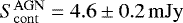 ,
,  , and
, and  . For the eastern lobe, we centered our measurement on the peak of the emission in our observations, while for the western lobe, where we do not have a clear peak, we centered on the radio peak.
Comparing the continuum emission from this work and the radio emission from Best et al. (1999) (white and blue contours in Fig. 4, respectively), we note that our brighter continuum component (~ 83% of the total continuum emission flux) roughly corresponds to the radio emission of the core and the western lobe (~ 65% at ν = 8210 MHz and 66% at ν= 4710 MHz of the total flux), and also includes the fainter part of the eastern jet. The peak of the continuum emission at 94.48 GHz is centered on the AGN (~71% of the total continuum emission flux), while most of the radio emission from Best et al. (1999) is from the western lobe (~ 52% at ν = 8210 MHz and 59% at ν = 4710 MHz of the total flux). Our fainter continuum component (~17% of the total flux) corresponds to the radio emission of the eastern lobe and a brighter part of the eastern jet (~ 35% at ν = 8210 MHz and 34% at ν= 4710 MHz of the total flux).
Table 1 shows our continuum flux measurements at 94.48 GHz, and those from Best et al. (1999) at 4.71 and 8.21 GHz. The total flux in the table is the sum of the three components, the core and the two lobes. The total flux measured in an area with the signal exceeding 3σ of the background is  . We modeled the AGN and lobe spectral energy distribution (SED) as a power law (Ssynch ∝ ν−α), and obtained the spectral index α for the different components from a linear fit in logarithmic scale, using all three frequencies. The uncertainty on α is the statistical uncertainty from the linear fit. The systematic uncertainty on αB99 of 0.07 from Best et al. (1999) is much larger than the statistical uncertainty and is calculated by assuming 3% uncertainties in the absolute calibration at each Best et al. (1999) frequency. Our indexes are consistent (1–1.5σ) with those from Best et al. (1999) (also shown in Table 1). The lobes present a steep SED, consistent with the optically thin synchrotron emission of the jets (Best et al. 1999; Laing & Bridle 2013; Nyland et al. 2017; Ruffa et al. 2019; Grossová et al. 2019), while the AGN core SED is flatter, which is consistent with optically thicker (self-absorbed) synchrotron emission (Best et al. 1999; Ruffa et al. 2019; Grossová et al. 2019).
In Fig. 5, we show the total AGN SED at radio and millimeter wavelengths from our work (total AGN emission) and the literature. Over this larger range of frequencies, we obtain α = 0.92 ± 0.02, consistent with the optically thin synchrotron emission of AGN jets that dominate the total continuum emission. The SED does not show a flattening or steepening at high-frequency (ν > 10 GHz) either, in agreement with previous results (Klamer et al. 2006; Emonts et al. 2011; Falkendal et al. 2019).
Our results are within the range of spectral indexes found in previous work. The typical spectral index of optically thin synchrotron emission (which corresponds to jets) is in the range of 0.5 ≲ α ≲ 1.5 in the local Universe (Laing & Bridle 2013; Nyland et al. 2017; Ruffa et al. 2019; Grossová et al. 2019) and 1 ≲ α ≲ 2 for galaxies at z > 2, with higher values being rarer (Carilli et al. 1997; Best et al. 1999; Falkendal et al. 2019). For the optically thick emission (which corresponds to the core), − 0.5 ≲ α ≲ 0.5 is found in the local Universe (Ruffa et al. 2019; Grossová et al. 2019) and − 1 ≲ α ≲ 1 is found at z > 2, with most of the measurements being α > 0.5 (Carilli et al. 1997; Athreya et al. 1997; Best et al. 1999; Falkendal et al. 2019).
Continuum flux measurements.
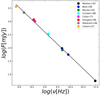 |
Fig. 5 Total SED plot of the AGN in the radio and millimeter wavebands from our work (black), Best et al. (1999) (blue), Becker et al. (1991) (green), Condon et al. (1998) (cyan), Colla et al. (1973) (magenta), Douglas et al. (1996) (red), Waldram et al. (1996) (gray), and Cohen et al. (2007) (orange). Over this range of frequencies, we obtain an AGN spectral index of α = 0.92 ± 0.02. |
3.2 Molecular gas content around the active galactic nucleus
System velocity and FWHM
In order to estimate the system velocity and the velocity full width at half maximum (FWHM) from the CO(2–1) line emission, weuse the class package from the GILDAS software. We extract the CO(2–1) line profile from a polygon enclosing all > 1σ CO(2–1) emission in the central region of the cluster.
In the integrated spectrum, we identify two emission lines, which we fit as Gaussians (Fig. 6, right). The two Gaussian emission peaks are at Vsys = −623 ± 30 km s−1 with a velocity of FWHM = 179 ± 71 km s−1, and Vsys = −116 ± 40 km s−1 with a velocity of FWHM = 346 ± 87 km s−1. We show these fits as the blue and the red Gaussians, respectively, in Fig. 6. The zero point Vsys = 0 km s−1 in the spectrum corresponds to a redshift of z = 1.44, approximately the mean confirmed cluster member redshift from Noirot et al. (2018), as explained in the observation section. In Appendix A, we identify the emission regions of the two CO(2–1) emission peaks by mapping the position of each component using the GILDAS software and we find that the two peaks correspond to two separate regions, one southeast and the other southwest of the AGN. Hereafter we identify the two peaks as the eastern and western emission peaks.
In Fig. 7, we compare the emission regions that we find from this analysis to the position of the CARLAIRAC color-selected galaxies in our HST/F140W image. We find that the spatial extension that corresponds to the eastern and western emission peaks is south of central AGN. Neither the eastern nor the western emission peaks correspond to the spatial position or to the spectroscopic redshift of the AGN (Fig. 6). The peaks do not correspond to any optical (HST/WFC3) or infrared (Spitzer/IRAC) counterpart.We remind the reader that the bright central source south of the AGN is a star and not a galaxy (see Sect. 2.2).
The other detections at the center of the NOEMA CO(2–1) line emission mosaic map (Fig. 3, right) are at S∕N ≤ 2. Their velocity peak is at the same spectral position as the western peak, and we again do not detect galaxies at their position in the HST/WFC3 or Spitzer/IRAC images. We conclude that those overdensities might be due to the side lobes, and neglect them. We do not have detections at >3σ at the edgesof the mosaic, where the noise is higher.
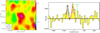 |
Fig. 6 Left: zoom-in on the CO(2–1) line emission, continuum-subtracted mosaic map of the extended source in the cluster center. The black cross marks the center of our observations. The beam size (4.14 × 3.45 arcsec2) is plotted at the lower left. The color scale of the intensity map is in Jy beam−1. The rms noise level is σ ~ 0.2 mJy beam−1 in the central pointing intersection region. The contours correspond to the 1σ, 2σ, and 3σ levels. Right: CO(2–1) line emission integrated spectrum. The two Gaussian fits correspond to system velocities of Vsys =−623.0 km s−1 (blue) and Vsys = −115.5 km s−1 (red). The AGN spectroscopic redshift corresponds to a velocity of v = 331.6 km s−1 (vertical green line). |
Flux and luminosity
From the Gaussian fit, the velocity-integrated flux for the eastern and western emission peaks are SCO(2−1)Δv = 0.6 ± 0.2 Jy km s−1 (S∕N ~ 3; here and hereafter the S/N is calculated as the signal divided by its uncertainty, before approximating to one significant figure), and SCO(2−1)Δv = 0.9 ± 0.2 Jy km s−1 (S∕N ~ 4), respectively. In the Gaussian fit, we leave all parameters free to vary. The uncertainty on the measurements includes the uncertainties in the Gaussian fit and the noise in the region in which the fit is performed. The total flux for the eastern emission peak, obtained by integrating over the velocity range − 1075 km s−1 < v < −475 km s−1, is SCO(2−1)Δv = 0.88 ± 0.16 Jy km s−1 (S/N ~ 6; Figs. 7 and A.2). The difference between this flux measurement and that obtained from the Gaussian fit is consistent with zero. The total flux for the western emission peak, obtained by integrating over the velocity range − 375 km s−1 < v < +125 km s−1, is SCO(2−1)Δv = 0.90 ± 0.15 Jy km s−1 (S/N ~ 6; Figs. 7 and A.3), and very similar to the value obtained from the Gaussian fit. The integrated flux from the eastern and western emission peaks over the velocity range − 1075 km s−1 < v < 125 km s−1 is SCO(2−1)Δv = 1.7 ± 0.2 Jy km s−1 (S/N ~ 10). We do not measure any CO(2–1) line emission at the spectral position of the AGN, z = 1.4427 ± 0.0005, which corresponds to a velocityof v = 331.6 km s−1, shown as a vertical green line in Fig. 6. Hereafter, we use the velocity integrated fluxes for both the eastern and western emission peaks, for which we have the higher S/N. We calculate the CO(2–1) luminosity using the following relation from Eq. (3) of Solomon & Vanden Bout (2005):
 (1)
(1)
where  is the CO(2–1) line luminosity in K km s−1 pc2, SCO(2−1)Δv is the CO(2–1) velocity integrated flux in Jy km s−1, DL = 10 397.4 Mpc is the AGN luminosity distance, νrest = 230.538 GHz is the rest frequency of the CO(2–1) rotational transition, and z = 1.4427 ± 0.0005 is the AGN redshift (see Sect. 2.2). We find
  and
and  , for the eastern and western emission peaks, respectively.
Molecular gas mass
In order to estimate the molecular gas mass, we use the mass-to-luminosity relation
 (2)
(2)
where Mgas is the molecular gas mass, αCO is the CO-to-H2 conversion factor (e.g., see review by Bolatto et al. 2013), r21 is the  luminosity ratio, and
  and
and  are the luminosities of the CO(2–1) and CO(1–0) emission lines, respectively.
We assume thermalized, optically thick CO emission for which the CO luminosities are independent of the rotational transitions, thus, 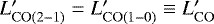 and r21 = 1 (Solomon & Vanden Bout 2005). This is a standard value used for the local galaxy M82 (Weiß et al. 2005) and for color-selected star-forming galaxies (CSGs, Dannerbauer et al. 2009). However other works use different values of r21, such as r21 = 0.5 for the Milky Way (Weiß et al. 2005). The reader should take into account these differences when comparing with other works in the literature (e.g., Casasola et al. 2013; Noble et al. 2017; Rudnick et al. 2017; Hayashi et al. 2018; Coogan et al. 2018; Castignani et al. 2018).
The CO-to-H2 conversion factor αCO is a large uncertainty in this calculation. Its value is not universal and depends on galaxy type, metallicity, and CO gas excitation temperature and density (Bolatto et al. 2013; Carilli & Walter 2013; Combes 2018). For different kinds of galaxies and environments, its average range of values is  (Bolatto et al. 2013). Since neither the eastern nor the western emission peaks are associated with galaxies detected in our optical and near-infrared images, they might be associated with extended emission around the AGN. In that case, we expect that the molecular gas might be more excited and have more chaotic motions, and this might lead to an expected value of r21 > 1, and to
  (Bolatto et al. 2013; Carilli & Walter 2013; Cicone et al. 2018). For these reasons, we use the lower end of standard αCO values, and this will give us lower limits to the molecular gas mass. When using
  , we obtain
 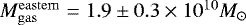 and
and 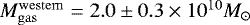 , for the eastern and western peak components, respectively. When using the Galactic conversion factor
  , the molecular gas masses are approximately five times larger. Summing the two components, the total molecular gas mass is
 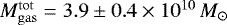 (S∕N ~ 8), and this mass is not spatially associated with galaxies detected in our optical or near-infrared images. Table 2 shows the integrated flux measurements, the CO luminosity, and the molecular gas mass.
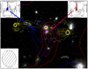 |
Fig. 7 HST/WFC3 F140W image of the central region of the cluster, with contours of CO(2–1) emission of the eastern and western emission peaks (shown as blue and red contours, respectively), and the radio emission at 4.71 GHz (yellow) from the work of Best et al. (1999). The central peak of the radio emission corresponds to the position of the AGN. The two radio lobes are asymmetrical, with the one to the east (left of the AGN) being more compact and the one to the west more diffuse. The central blue square and the pink star with four spikes show the position of the AGN and of the star, respectively. The green squares are the positions of IRAC color-selected galaxies in the cluster’s central region. The contours are derived by integrating the CO(2–1) emission across the velocities marked by their corresponding color on the CO(2–1) emission line spectra. The spectra are shown in the top left and right insets (see Appendix A for more details). The contour levels of the eastern and western emission peaks are 1–2σ and 1–4σ, respectively. The eastern and western emission peaks are south of the AGN, and do not correspond to any galaxy detected on the HST or Spitzer images. North is up and east is to the left. The beam scale is shown on the bottom left. |
3.3 Molecular gas content and star formation in cluster core members
We present the star formation properties of spectroscopically confirmed cluster members that are in the region covered by the NOEMA observations. We measure the upper limits on the molecular gas content of the confirmed cluster members and their star formation rates. We derive the galaxy gas fraction, and specific star formation rate (sSFR), and gas depletion time and star formation efficiency (SFE) upper limits.
Integrated flux measurements, the CO luminosity, and the gas mass from the integrated CO(2–1) line emission.
3.3.1 Upper limits on the molecular gas content of the confirmed cluster members
Besides the AGN, there are seven other spectroscopically confirmed CARLA J1103 + 3449 cluster members (Noirot et al. 2018), of which six are within the NOEMA beam, and three have stellar mass estimates (Fig. 2). Our NOEMA observations do not show CO(2–1) emission with S∕N > 3 at the positions of the spectroscopically confirmed members. However, we can use the 3σ values of the flux rms noise level around the position of each confirmed cluster member to derive an upper limit on the velocity integrated flux SCO(2−1)Δv = (3σrms)Δv. As Δv, we used an average Δv = 300 km s−1, following Saintonge et al. (2017). Since the velocity resolution of our CO(2–1) map has an uncertainty of σΔv = 100 km s−1, the velocity range within 300 ± 3σΔv km s−1 includes most of the published Δv for star-forming cluster galaxies at these redshifts (e.g., Noble et al. 2017; Lee et al. 2017; Castignani et al. 2018; Hayashi et al. 2018). For the molecular gas measurement, we use the Galactic conversion factor  , as typical for normal galaxies (Bolatto et al. 2013; Carilli & Walter 2013; Combes 2018). The estimated physical properties of the spectroscopically confirmed members are given in Table 3.
3.3.2 Star formation rates
We calculate galaxy star formation rates using the Hα emission line flux from Noirot et al. (2018). We then combine them with our measurements of the molecular gas mass from the CO(2–1) line emission, and the galaxy stellar masses from Mei et al. (in prep.), in order to estimate the galaxy gas fraction, and sSFR, and depletion time and SFE upper limits.
Galaxy stellar masses and gas fractions
Mei et al. (in prep.) describe the details of our stellar mass measurements. We measure our CARLA galaxy stellar masses by calibrating our PSF-matched Spitzer IRAC1 magnitudes (Amodeo et al., in prep.) with galaxy stellar masses from Santini et al. (2015) derived from the Guo et al. (2013) multiwavelength catalog in the Cosmic Assembly Near-infrared Deep Extragalactic Legacy Survey (CANDELS; PI: S. Faber, H. Ferguson; Koekemoer et al. 2011; Grogin et al. 2011) WIDE GOODS-S field.
The Spitzer IRAC1 magnitudes correspond to the rest-frame near infrared in the redshift range of the CARLA sample, and we expect them not to be biased by extinction. We find a very good correlation between these magnitudes and the Santini et al. (2015) mass measurements, with scatters of ~ 0.12 dex at the redshift of the cluster studied in this paper. Adding in quadrature the scatter of the relation and uncertainties from Santini et al. (2015), we obtain mass uncertainties in the range ~ 0.4–0.5 dex, and ~ 0.2–0.3 dex for masses larger than log .
.
Table 3 shows the stellar masses of the spectroscopically confirmed cluster members. The masses derived from this calibration are on average ~0.5 dex smaller to those derived from stellar population models by Noirot et al. (2018), and the difference is larger at fainter magnitudes.This difference in mass estimates does not significantly change results from Noirot et al. (2018), in particular the conclusions from the SFR versus stellar mass analysis (Fig. 7 in Noirot et al. 2018). From our molecular gas mass upper limits, combined with our stellar masses, we compute the gas-to-stellar mass ratio as Mgas∕M* and the molecular gas fraction as fgas = Mgas∕(Mgas + M*). The results are shown in Table 3.
Star formation rates, specific star formation rates, depletion times and star formation efficiencies
We re-compute SFRHα, using the Hα line fluxes from Noirot et al. (2018) and our stellar masses from Mei et al. (in prep.). The Kennicut law (Kennicutt 1998) shows a direct proportionality between SFR and Hα flux,
![Mathematical equation: \begin{equation*}\textrm{SFR}_{\textrm{H}{\alpha}} [M_{\odot} \rm{yr}^{-1}] = 5 \times 10^{-42} \textit{L}_{\rm{H}{\alpha}} \times 10^{0.4 \times {\textit{A}}_{\rm{H}{\alpha}}} ,\end{equation*}](/articles/aa/full_html/2020/09/aa38673-20/aa38673-20-eq24.png) (3)
(3)
where SFRHα is the estimated SFR corrected for the contribution from the [NII] line and AHα is the dust attenuation.
We estimate AHα using the Garn & Best (2010) empirical law (which used the Calzetti et al. 2000 extinction law),
 (4)
(4)
where  and M* is the stellar mass.
The symbol LHα represents the Hα luminosity in erg s−1, and it is calculated from FHα, the Hα flux given in erg cm−2 s−1, which is computed as
![Mathematical equation: \begin{equation*}F_{\textrm{H}{\alpha}} = F_{\textrm{H}{\alpha} + [\textrm{NII}] \lambda 6548, 6584}\frac{1}{1 + \frac{F_{[\textrm{NII}] \lambda 6548, 6584}}{F_{\textrm{H}{\alpha}}}} ,\end{equation*}](/articles/aa/full_html/2020/09/aa38673-20/aa38673-20-eq27.png) (5)
(5)
where FHα+[NII]λ6548,6584 is the total observed Hα flux plus the [NII]λ6548, 6584 flux. In fact,the WFC3/G141 grism resolution does not permit us to deblend the three lines (Noirot et al. 2018). To measure ![Mathematical equation: ${\frac{{F}_{\textrm{[NII] \lambda 6548, 6584}}}{{F}_{\textrm{H}{\alpha}}}}$](/articles/aa/full_html/2020/09/aa38673-20/aa38673-20-eq28.png) , we use the relation between this ratio and metallicity, and the fundamental relation between stellar mass, SFR, and metallicity. Following Curti et al. (2020) (Eqs. (2) and (5) and Table 6), we calculate the metallicity 12 + log(O∕H), expressed as a function of stellar mass and SFR:
, we use the relation between this ratio and metallicity, and the fundamental relation between stellar mass, SFR, and metallicity. Following Curti et al. (2020) (Eqs. (2) and (5) and Table 6), we calculate the metallicity 12 + log(O∕H), expressed as a function of stellar mass and SFR:
![Mathematical equation: \begin{equation*}\begin{aligned} \rm{12 + log(O/H)}= Z_0 - \gamma/\beta \times log \left[1 + \left(\frac{\textit{M}_*}{\textit{M}_0(\rm{SFR})}\right)^{-\beta}\right] \end{aligned} ,\end{equation*}](/articles/aa/full_html/2020/09/aa38673-20/aa38673-20-eq29.png) (6)
(6)
where Z0 = 8.779 ± 0.005, log (M0(SFR)) = m0 + m1 ×log(SFR), m0 = 10.11 ± 0.03, m1 = 0.56 ± 0.01, γ = 0.31 ± 0.01, and β = 2.1 ± 0.4.
Curti et al. (2020) also provide a new calibration for the relation between metallicity and ![Mathematical equation: ${\frac{{F}_{\textrm{[NII]}_{\lambda6584}}}{{F}_{\textrm{H}{\alpha}}}}$](/articles/aa/full_html/2020/09/aa38673-20/aa38673-20-eq30.png) :
:
![Mathematical equation: \begin{equation*}\textrm{log}\left( {\frac{{F}_{\textrm{[NII]}_{\lambda6584}}}{{F}_{\textrm{H}{\alpha}}}}\right) = \sum_{n=1}^{4} c_n x^n ,\end{equation*}](/articles/aa/full_html/2020/09/aa38673-20/aa38673-20-eq31.png) (7)
(7)
where x = 12 + log(O/H) − 8.69, c0 = −0.489, c1 = 1.513, c2 = −2.554, c3 = −5.293, and c4 = −2.867. Assuming a constant ratio ![Mathematical equation: ${{F}_{\textrm{[NII]}_{\lambda6584}}}$](/articles/aa/full_html/2020/09/aa38673-20/aa38673-20-eq32.png) :
:![Mathematical equation: ${{F}_{\textrm{[NII]}_{\lambda6548}}}$](/articles/aa/full_html/2020/09/aa38673-20/aa38673-20-eq33.png) of 3:1 (Osterbrock & Ferland 2006), we derive
of 3:1 (Osterbrock & Ferland 2006), we derive ![Mathematical equation: $ {\frac{{F}_{\textrm{[NII]} \lambda 6548, 6584}}{{F}_{\textrm{H}{\alpha}}}}$](/articles/aa/full_html/2020/09/aa38673-20/aa38673-20-eq34.png) .
.
Since to calculate SFR in Eq. (3) we need to know ![Mathematical equation: ${\frac{{F}_{\textrm{[NII]} \lambda 6548, 6584}}{{F}_{\textrm{H}{\alpha}}}}$](/articles/aa/full_html/2020/09/aa38673-20/aa38673-20-eq35.png) , and to measure
, and to measure ![Mathematical equation: ${\frac{{F}_{\textrm{[NII]} \lambda 6548, 6584}}{{F}_{\textrm{H}{\alpha}}}}$](/articles/aa/full_html/2020/09/aa38673-20/aa38673-20-eq36.png) in Eq. (7) we need to know the SFR, we follow Zeimann et al. (2013) and start with an initial value of
in Eq. (7) we need to know the SFR, we follow Zeimann et al. (2013) and start with an initial value of ![Mathematical equation: $ {\frac{{F}_{\textrm{[NII]} \lambda 6548, 6584}}{{F}_{\textrm{H}{\alpha}}}}=0.2$](/articles/aa/full_html/2020/09/aa38673-20/aa38673-20-eq37.png) and iterate Eqs. (3)–(7) until convergence.
and iterate Eqs. (3)–(7) until convergence.
Our results are shown in Table 4. For the AGN, we cannot separate the stellar contribution to the Hα+[NII] line emission from the AGN contribution (Tadhunter 2016). Since we know that the hosts of powerful AGNs present young stellar populations (e.g., Heckman & Kauffmann 2006), we consider that the stellar contribution to the total Hα+[NII] emission varies in the range of 20–100%. In Table 4, we compare our SFR measurements with those from Noirot et al. (2018), and we are consistent within 1.5–2σ. For some cluster galaxies we could not measure stellar masses, because they are not detected in the IRAC images, and we cannot re-compute the SFR. Hereafter, we will use our SFR measurements when we could derive them, and Noirot et al. (2018) SFR measurements for the other galaxies. Combining our measured SFR with the stellar masses from Mei et al. (in prep.), we compute the specific star formation rate  , the depletion time
  , and the star formation efficiency
  . Our results are shown in Table 4.
Velocity integrated CO(2–1) flux, luminosity, molecular gas mass, stellar mass, molecular gas-to-stellar mass ratio, and molecular gas fraction for the CARLA J1103 + 3449 cluster confirmed members.
CARLA J1103 + 3449 cluster confirmed member  , attenuation, metallicity, SFR, sSFR, depletion time, and SFE.
4 Discussion
In this section, we discuss our results. We focus on understanding the origin of the molecular gas in the cluster central region and on the physical properties and scaling relations of the confirmed cluster members.
4.1 Origin of the molecular gas in the cluster core
In the core of the cluster, we observe two CO(2–1) emission peaks that correspond to a region spatially offset from the center of the AGN continuum emission and that does not correspond to any galaxy detected in our HST or Spitzer images. Radio observations of the CARLA J1103 + 3449 cluster from the work of Best et al. (1999) reveal two radio lobes, which are roughly in the same directions (east and west) as our CO(2–1) molecular gas components and our data extended continuum emission (Figs. 4, 7, and 8). The two radio lobes are asymmetrical, the western being more compact, while the eastern is more diffuse. The asymmetry of their widths may be due to their expansion in an ICM (intracluster medium) with a density gradient, in which the more diffuse lobe, the western lobe, would be expanding in a less dense environment (e.g., Seymour et al. 2020). Both CO(2–1) emission peaks are blueshifted compared to the NOEMA observation central velocity of 0 km s−1 (which corresponds to the cluster redshift of z = 1.44) and to the AGN redshift, and their spatial position is close to, but south of the AGN and the radio lobes.
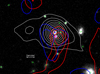 |
Fig. 8 HST/WFC3 F140W image of the central region of the cluster, with the contours of CO(2–1) emission of the eastern (1–2σ) and western (1–4σ) emission peaks (shown as blue and red contours, respectively), and the continuum emission at 94.5 GHz (white contours; 3–24σ). The central blue square and the pink star with four spikes show the position of the AGN and of the star, respectively. The green squares are the positions of IRAC color-selected galaxies in the cluster’s central region. North is up and east is to the left. |
4.1.1 Undetected galaxies
To exclude the hypothesis that the two CO(2–1) line emission components might originate from two or more galaxies that are not detected at the detection limit of our optical or near infrared images, we measure their hypothetical properties by making reasonable assumptions. Since our HST/WFC3 F140W images have a depth similar to the CANDELS WIDE survey, we use the CANDELS/WIDE survey mass limit M* = 5 × 10⁹ M⊙ (Grogin et al. 2011; similar to our Spitzer mass limit) as an upper limit to the stellar mass of each of these two hypothetical galaxies.
Assuming the 3σ Hα emission line flux limit of FHα = 2.1 × 10⁻¹⁷ erg cm−2 s−1 for the HST/WFC3 G141 grism spectra (Momcheva et al. 2016; Noirot et al. 2018) as an upper limit of the undetected Hα flux, and using the upper limit of the stellar mass, we estimate an upper limit to the SFR of the two emission peak components as SFRHα < 2 M⊙ yr−1, using the same system of equations in Sect. 3.3.2 and the cluster redshift2. We then estimate lower limits to the molecular gas-to-stellar mass ratios and gas fractions that correspond to the eastern and western peak emission. We obtain molecular gas masses of 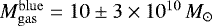 , and
, and  . We use the Galactic conversion factor because it is very improbable that these hypothetical galaxies are star-burst galaxies since they are not detected in our HST/WFC3 G141 grism observations. They could be only if the attenuation has an anomalously high values, of AHα > 5. Those gas masses lead to estimated gas fraction lower limits of fgas ≳ 95%, and a lower limit on the depletion times of τdep ≳ 55 Gyr. This is much longer than the depletion times observed for standard star-forming galaxies up to z ~ 4, which are closer to ~1−3 Gyr (e.g., Tacconi et al. 2013, 2018). The probability that the line that we are observing is not CO(2–1) is very small, given that it is very close to the CO(2–1) emission expected at the cluster redshift.
Some massive galaxies at z > 2 can be detected in millimeter wavelengths but not in the HST optical and near-infrared bands (e.g., Franco et al. 2018). However, these galaxies are rare (0.1 galaxy arcmin−2), massive, and usually detected with Spitzer/IRAC. Given the number densities of high redshift galaxies (e.g., Davidzon et al. 2018; Franco et al. 2018), having two galaxies of this kind so spatially close is possible but very improbable. These results mean that these two hypothetical galaxies would be unusually gas rich, with low SFR (or anomalously high attenuation), high gas fractions, and very long depletion times, independent of the conversion factor that we use. It is then very unlikely that our signal is due to undetected galaxies.
4.1.2 Extended emission
Excluding the hypothesis that the two CO(2–1) emission lines are due to undetected galaxies, they might trace molecular gas originating from an extended disk or torus, or emission components of molecular gas outflows or inflows associated with the AGN and its two radio jet lobes. We find no evidence to support the hypothesis of CO emission from an extended (up to tens of kiloparsecs) rotating disk or torus of molecular gas around the AGN. In fact, the CO(2–1) eastern and western peak emissions are not spatially located at the AGN position, they are located southeast and southwest of the AGN and the radio jets. The total molecular gas mass in the southern structures around the AGN is ≿ 60% of the total molecular gas, from  , and the upper limit on the AGN molecular gas mass (<3 × 10¹⁰ M⊙; Sect. 3.2; Table 3).
In the local Universe, both disk-dominated and filament-dominated central cluster galaxies have been observed with the Atacama Large Millimeter/submillimeter Array (ALMA; Russell et al. 2019; Olivares et al. 2019). In the first type, most of the molecular gas is concentrated in a disk around the central galaxy, while in the second type the molecular gas is mostly (> 70%) in filaments around the central galaxy (the most known example being the Perseus cluster; Salomé et al. 2006). The filaments typically extend from a few kiloparsecs in length up to 10− 20 kpc, and the molecular gas emission is offset with respect to the central AGN by projected distances of a few kiloparsecs. For the central galaxy of the cluster A1795, some molecular gas clumps are associated with the lobes of the radio jets. In filament-dominated galaxies, the filaments trace radio bubbles, and are associated with both gas outflow and inflow.
The molecular gas that we detect south of our central AGN also dominates the cluster central molecular gas reservoir and our observations are consistent with the filament-dominated local central galaxies. This suggests that the eastern and western emission peaks can be associated with gas outflow and inflow from the AGN. In fact, the AGN jets can drive a large amount of molecular gas, but this is not always expelled from the galaxy surroundings (e.g., Costa et al. 2015; Prasad et al. 2015), and can be re-accreted. As a consequence, the signal that we observe can be due to both inflows and outflows. When the amount of molecular gas outside the host galaxy is comparable to or higher than the host galaxy molecular gas reservoir, this also suggests that the gas has been cooled (e.g., Klamer et al. 2004; Nesvadba et al. 2009; Emonts et al. 2014; Russell et al. 2019). For the CARLA J1103 + 3449 cluster, we expect a reservoir of hot ICM that surrounds the host AGN, with accretion at the center of the cluster potential well. The detection of cool molecular gas around a central cluster AGN can indicate cooling due to the interaction of the ICM and AGN jets or can be due to condensation of low entropy hot gas uplifted by the AGN jet away from the host galaxy (Salomé et al. 2006; Lim et al. 2008; Gaspari et al. 2012; McNamara et al. 2014; Russell et al. 2014; Emonts et al. 2014; Li et al. 2015; Prasad et al. 2015; Gaspari & Sa̧dowski 2017; Voit et al. 2017; Tremblay et al. 2018; Olivares et al. 2019). With our observations, we cannot distinguish between these two scenarios.
4.2 Confirmed cluster member physical properties and scaling relations
In this section, we compare the physical properties of our measured cluster confirmed members to both cluster and field galaxies at similar redshifts (1 < z < 2.6). Our CO(2–1) luminosity, estimated upper limits to the velocity integrated CO(2–1) flux, and depletion times are similar to the literature for other cluster galaxies, AGN, and spiral galaxies at 1 < z < 2.5 (Wagg et al. 2012; Casasola et al. 2013; Emonts et al. 2014; Rudnick et al. 2017; Noble et al. 2017; Castignani et al. 2018, 2020; Hayashi et al. 2018), and galaxies in the field in the same redshift range (Tacconi et al. 2013). To compare our molecular gas upper limits to the literature, we have to take into account that we assume  (Sect. 3; Solomon & Vanden Bout 2005), and in several works a lower ratio of ~ 20−50% is assumed. For example, Noble et al. (2017) use a ratio of
  , Hayashi et al. (2018) use
  , and Tacconi et al. (2013) assume
  . In Figs. 9–11, we show the original published values, without scaling. In fact, our results do not significantly change when using other values of
  . We also know that stellar mass estimations can differ by up to a factor of ~ 1.5−6 (~ 0.1−0.8 dex) when using different techniques or different stellar population models (van der Wel et al. 2006; Lee et al. 2009; Maraston et al. 2010; Raichoor et al. 2011; Pforr et al. 2012; Sorba & Sawicki 2018).
In Fig. 9, we compare our molecular gas mass versus stellar mass relation to other works. Our upper limits agree with the field molecular gas mass-to-stellar mass ratio from the Plateau de Bure high-z Blue Sequence Survey (PHIBBS) survey (Tacconi et al. 2013). This result also holds when considering the uncertainties in the  conversion, conversion factor αCO, and stellar masses. Our galaxies show upper limits that are higher than the molecular gas mass-to-stellar mass ratio in some of the other clusters. However, since they are only upper limits, we cannot make conclusions on environmental effects, apart from the fact that our cluster galaxies do not show evidence for larger gas reservoirs than field galaxies with similar stellar masses.
In Figs. 10 and 11, we show SFR as a function of stellar and molecular gas mass, respectively. Figure 10 only shows results for galaxies for which we can measure the stellar mass. Compared to field galaxies, the SFR of the AGN host is within ~ 1−1.5σ of the MS from Tacconi et al. (2013), and the SFR of the other spectroscopically confirmed cluster members is ~ 2σ lower than the MS (Fig. 10), consistent with results from Noirot et al. (2018), which concluded that star-forming galaxies with stellar mass > 1010 M⊙ in the CARLA HST cluster sample have lower SFR than field galaxies with similar masses at the same redshifts. In Fig. 11, the AGN SFR (for all the Hα stellar emission percentages considered in this paper) is also within ~ 1σ of field galaxies with gas masses similar to its molecular gas mass upper limit. This shows that its SFR is typical of galaxies in the field with the same molecular gas reservoir.
The AGN SFR is comparable to the main sequence of star-forming field galaxies, and its star formation has not yet been quenched. This is consistent with the large molecular gas reservoir in the center of the cluster. As a massive early-type central cluster galaxy, the AGN is predicted to have gone through at least one major merger, which might have triggered a starburst phase (Hopkins et al. 2006b, 2008; Snyder et al. 2011; Yesuf et al. 2014), which we do not observe as on-going in our data. During this phase, the galaxy is predicted to lie above the MS in the SFR−M* and SFR−Mgas diagrams (Figs. 10 and 11), and the galaxy molecular gas is converted into stars. Afterwards, the remaining molecular gas content is expected to be consumed by the combination of star formation and feedback (Snyder et al. 2011; Yesuf et al. 2014). Our AGN is observed on the star-forming galaxy MS (with a SFR of ~ 30–140 M⊙ yr−1), and we expect that it will evolve toward quenching when the molecular gas reservoir is depleted, becoming a passive ETG similar to those observed in lower redshift cluster centers (Norton et al. 2001; Hopkins et al. 2008; Snyder et al. 2011; Yesuf et al. 2014).
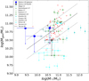 |
Fig. 9 Molecular gas mass vs. stellar mass relation for the AGN (empty black circles) and for other CARLA J1103 + 3449 spectroscopically confirmed cluster members (blue filled circles) compared to other cluster (green and cyan) and field galaxies (red) from the literature. The arrows show lower and upper limits. Green markers are the results for cluster galaxies for which gas masses were estimated using the Galactic conversion factor. Cyan markers are estimations with different values of the conversion factor. Dashed and dashed-dotted lines represent the Tacconi et al. (2013) relation for field star-forming galaxies and its 1σ scatter. |
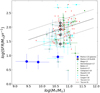 |
Fig. 10 Star formation rate as a function of stellar mass. Symbols are the same as in Fig. 9. The AGN SFR is shown with different contributions of the Hα+[NII] stellar emission to the total flux. We compare our results with those from other works. The dashed and the dashed-dotted lines represent the best fit with 1σ scatter for the MS of field galaxies from Tacconi et al. (2013). |
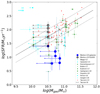 |
Fig. 11 Star formation rate as a function of gas mass. Symbols are the same as in Fig. 9. The arrows show upper limits. Dashed and dashed-dotted lines represent the Tacconi et al. (2013) relation for field star-forming galaxies and its 1σ scatter. |
5 Summary
We report on observations of the central region of the galaxy cluster CARLA J1103 + 3449 at z = 1.44 with NOEMA, and measure the molecular gas content in the center of the cluster. We also obtain SFR, sSFR, molecular gas mass, and SFE, and gas depletion time upper limits for the spectroscopically confirmed cluster members.
Our main results are:
-
At the rest frequency of νrest = 230.5 GHz, the dominant source of our NOEMA extended continuum emission is the non-thermal synchrotron radio emission from the AGN. We measured its flux at the AGN position and at the position of two radio jets. The central AGN in CARLA J1103 + 3449 has been already observed at 4.71 and 8.21 GHz by Best et al. (1999), who found two asymmetrical radio lobes, one oriented toward the east and the other toward the west. We measured the continuum within a region the size of the NOEMA beam centered on the AGN and the two lobes, and obtained
 ,
,
 , and
, and  . Combining our measurements with published results over the range 4.71–94.5 GHz, and assuming
Ssynch ∝ ν−α, we obtained a flat spectral index α = 0.14 ± 0.03 for the AGN core emission, and a steeper index α = 1.43 ± 0.04 and α = 1.15 ± 0.04 at positions close to the western and eastern lobe, respectively, which is consistent with optically thicker synchrotron emission. The total spectral index is α = 0.92 ± 0.02 over the range 73.8 MHz–94.5 GHz.
. Combining our measurements with published results over the range 4.71–94.5 GHz, and assuming
Ssynch ∝ ν−α, we obtained a flat spectral index α = 0.14 ± 0.03 for the AGN core emission, and a steeper index α = 1.43 ± 0.04 and α = 1.15 ± 0.04 at positions close to the western and eastern lobe, respectively, which is consistent with optically thicker synchrotron emission. The total spectral index is α = 0.92 ± 0.02 over the range 73.8 MHz–94.5 GHz. -
We detected two CO(2–1) emission line peaks with S∕N ~ 6, blueshifted with respect to the AGN redshift. One of the two detected emission peaks is situated at a projected distance of ~17 kpc southeast of the AGN, and the second one is ~14 kpc southwest of the AGN. These regions are roughly aligned with the radio jets (east-west), and south of them. These two emissions do not correspond to the position of any galaxy that we detect in our optical or near-infrared images, and it is very unlikely that they are due to undetected galaxies (see Sect. 4).
-
We found a massive reservoir of cool molecular gas in the center of the cluster, distributed south of the AGN. From the CO(2–1) total velocity integrated flux, the total cluster core molecular gas mass is
 . The two CO(2–1) emission line peaks correspond to molecular gas masses of Mgas = 1.9 ± 0.3 × 10¹⁰ M⊙
for the eastern component, and of Mgas = 2.0 ± 0.3 × 10¹⁰ M⊙
for the western component. Considering the upper limit of 3 × 10¹⁰ M⊙
on the AGN molecular mass (see below), the southern emission molecular gas mass is ≿60% of the cluster total central molecular mass reservoir. Our observations can be explained by gas inflows and outflows, either due to cluster gas accretion or, most probably, driven by the jets, as is observed in filament-dominated central galaxies in the local Universe. The gas might be cooled by the interaction of the ICM and AGN jets or could be due to condensation of low entropy hot gas uplifted by the AGN jet away from the host galaxy.
. The two CO(2–1) emission line peaks correspond to molecular gas masses of Mgas = 1.9 ± 0.3 × 10¹⁰ M⊙
for the eastern component, and of Mgas = 2.0 ± 0.3 × 10¹⁰ M⊙
for the western component. Considering the upper limit of 3 × 10¹⁰ M⊙
on the AGN molecular mass (see below), the southern emission molecular gas mass is ≿60% of the cluster total central molecular mass reservoir. Our observations can be explained by gas inflows and outflows, either due to cluster gas accretion or, most probably, driven by the jets, as is observed in filament-dominated central galaxies in the local Universe. The gas might be cooled by the interaction of the ICM and AGN jets or could be due to condensation of low entropy hot gas uplifted by the AGN jet away from the host galaxy. -
The central AGN host is an ETG with a SFR of ~30−140 M⊙ yr−1, depending on the assumed percentage of AGN contribution to its Hα+[NII] flux (20–100%). The upper limit on its gas reservoir is of Mgas < 3 × 10¹⁰ M⊙. This means that the AGN molecular gas reservoir amounts to ≲40% of the total molecular gas reservoir in the center of the cluster. The AGN host SFR lies on the MS of star-forming galaxies at a similar redshift, and it has not yet been quenched. We expect that its star formation will be also fed by the larger southern molecular gas reservoir.
-
We measured SFR and sSFR, and estimated upper limits on the molecular gas masses, gas fractions, SFE, and depletion times for the other spectroscopically confirmed cluster members. Our spectroscopically confirmed cluster member SFR is at ~2σ below the field star-forming MS (Fig. 10), consistent with results from Noirot et al. (2018), who concluded that star-forming galaxies with stellar mass >1010 M⊙ in the CARLA HST cluster sample have a lower SFR than field galaxies at a similar redshift, and of similar stellar mass. We find that the molecular gas mass upper limits are in the range of average values for field galaxies at similar redshiftsand of similar stellar mass, and we cannot make conclusions on environmental effects apart from the fact that our cluster galaxies do not show evidence for larger gas reservoir than field galaxies with similar stellar mass.
Acknowledgments
We thank the PI: of the Keck observations, Fiona Harrison, for providing these observations and Thomas Connor for assisting with the Keck observing. We thank Philip Best and Katherine Inskip for useful discussion and their kind sharing of their radio, optical and infrared observations of the central radio sources and lobes. The data reduction and mapping and most of data analysis was done by using IRAM/GILDAS free software (http://www.iram.fr/IRAMFR/GILDAS/), and with the assistance of the IRAM support astronomers in Grenoble, Cynthya Herrera and Melanie Krips, which we warmly thank. We would like to thank the GILDAS support team for their help and guidance forthe data analysis, Sébastien Bardeau and Vincent Pietu. V.M. would like to thank Anelise Audibert, Benoit Tabone, Valeria Olivares and Gianluca Castignani for their help with the data mapping and analysis. The work of D.S. was carried out at the Jet Propulsion Laboratory, California Institute of Technology, under a contract with NASA. This work was supported by the CNES.
Appendix A Positions of the two CO(2–1) emission peaks
In order to kinematically resolve the two components of the CO(2–1) emission line, we performed an analysis of different ranges of channels (velocities or frequencies) in the CO(2–1) spectrum and created the corresponding CO(2–1) emission line intensity maps, averaged over the chosen range of velocities. In Fig. A.1, we select a range of velocities so that we include both the eastern and western emission peaks (− 1075 km s−1 < v < +125 km s−1. In Fig. A.2, we select only the range of velocities that correspond to the eastern peak (− 1075 km s−1 < v < −475 km s−1). In Fig. A.3, we select only the range of velocities that correspond to the western peak (− 375 km s−1 < v < +125 km s−1). We can see that, although both the eastern and western emission peaks are superposed in some regions of the cluster core, we can kinematically separate them.
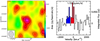 |
Fig. A.1 Left: CO(2–1) line emission intensity map of the central cluster region with NOEMA created by selecting the channel ranges that include both the eastern and western emission peaks (on the right). The spectra are binned in channels of 100 km s−1. The contour levels are 1σ, 2σ, and 3σ. |
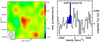 |
Fig. A.2 Left: CO(2–1) line emission intensity map of the central cluster region with NOEMA created by selecting the channel ranges that include only the eastern emission peak (on the right). The spectra are binned in channels of 100 km s−1. The contour levels are 1σ and 2σ. |
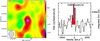 |
Fig. A.3 Left: CO(2–1) line emission intensity map of the central cluster region with NOEMA created by selecting the channel ranges that include only the western emission peak (on the right). The spectra are binned in channels of 100 km s−1. The contour levels are 1σ, 2σ, 3σ, and 4σ. |
References
- Abadi, M. G., Moore, B., & Bower, R. G. 1999, MNRAS, 308, 947 [NASA ADS] [CrossRef] [Google Scholar]
- Abdo, A. A., Ackermann, M., Ajello, M., et al. 2010, ApJ, 710, 133 [NASA ADS] [CrossRef] [Google Scholar]
- Alberts, S., Pope, A., Brodwin, M., et al. 2016, ApJ, 825, 72 [NASA ADS] [CrossRef] [Google Scholar]
- Aloy, M.-A., Gómez, J.-L., Ibáñez, J.-M., Martí, J.-M., & Müller, E. 2000, ApJ, 528, L85 [Google Scholar]
- Athreya, R. M., Kapahi, V. K., McCarthy, P. J., & van Breugel, W. 1997, MNRAS, 289, 525 [NASA ADS] [CrossRef] [Google Scholar]
- Baldry, I. K., Balogh, M. L., Bower, R. G., et al. 2006, MNRAS, 373, 469 [NASA ADS] [CrossRef] [Google Scholar]
- Balogh, M. L., & Morris, S. L. 2000, MNRAS, 318, 703 [Google Scholar]
- Balogh, M. L., Schade, D., Morris, S. L., et al. 1998, ApJ, 504, L75 [NASA ADS] [CrossRef] [Google Scholar]
- Balogh, M., Eke, V., Miller, C., et al. 2004, MNRAS, 348, 1355 [Google Scholar]
- Bassett, R., Papovich, C., Lotz, J. M., et al. 2013, ApJ, 770, 58 [NASA ADS] [CrossRef] [Google Scholar]
- Becker, R. H., White, R. L., & Edwards, A. L. 1991, ApJS, 75, 1 [Google Scholar]
- Bertin, E., & Arnouts, S. 1996, A&AS, 117, 393 [NASA ADS] [CrossRef] [EDP Sciences] [Google Scholar]
- Best, P. N., Eales, S. A., Longair, M. S., Rawlings, S., & Rottgering, H. J. A. 1999, MNRAS, 303, 616 [NASA ADS] [CrossRef] [Google Scholar]
- Binney, J., & Tremaine, S. 1987, Galactic dynamics (Princeton: Princeton University Press) [Google Scholar]
- Bisbas, T. G., van Dishoeck, E. F., Papadopoulos, P. P., et al. 2017, ApJ, 839, 90 [NASA ADS] [CrossRef] [Google Scholar]
- Bolatto, A. D., Wolfire, M., & Leroy, A. K. 2013, ARA&A, 51, 207 [Google Scholar]
- Boselli, A., & Gavazzi, G. 2006, PASP, 118, 517 [NASA ADS] [CrossRef] [Google Scholar]
- Bregman, J. N. 1990, A&ARv, 2, 125 [NASA ADS] [CrossRef] [Google Scholar]
- Brodwin, M., Stanford, S. A., Gonzalez, A. H., et al. 2013, ApJ, 779, 138 [NASA ADS] [CrossRef] [Google Scholar]
- Calzetti, D., Armus, L., Bohlin, R. C., et al. 2000, ApJ, 533, 682 [NASA ADS] [CrossRef] [Google Scholar]
- Carilli, C. L., & Walter, F. 2013, ARA&A, 51, 105 [NASA ADS] [CrossRef] [EDP Sciences] [Google Scholar]
- Carilli, C. L., Röttgering, H. J. A., van Ojik, R., Miley, G. K., & van Breugel, W. J. M. 1997, ApJS, 109, 1 [NASA ADS] [CrossRef] [Google Scholar]
- Carleton, T., Errani, R., Cooper, M., Kaplinghat, M., & Peñarrubia, J. 2019, MNRAS, 485, 382 [NASA ADS] [CrossRef] [Google Scholar]
- Casasola, V., Magrini, L., Combes, F., et al. 2013, A&A, 558, A60 [NASA ADS] [CrossRef] [EDP Sciences] [Google Scholar]
- Castignani, G., Combes, F., Salomé, P., et al. 2018, A&A 617, A103 [NASA ADS] [CrossRef] [EDP Sciences] [Google Scholar]
- Castignani, G., Pandey-Pommier, M., Hamer, S. L., et al. 2020, A&A, 640, A65 [CrossRef] [EDP Sciences] [Google Scholar]
- Chabrier, G. 2003, PASP, 115, 763 [Google Scholar]
- Chapman, S. C., Bertoldi, F., Smail, I., et al. 2015, MNRAS, 449, L68 [Google Scholar]
- Chiang, Y.-K., Overzier, R. A., Gebhardt, K., & Henriques, B. 2017, ApJ, 844, L23 [NASA ADS] [CrossRef] [Google Scholar]
- Cicone, C., Severgnini, P., Papadopoulos, P. P., et al. 2018, ApJ, 863, 143 [NASA ADS] [CrossRef] [Google Scholar]
- Cohen, A. S., Lane, W. M., Cotton, W. D., et al. 2007, AJ, 134, 1245 [NASA ADS] [CrossRef] [Google Scholar]
- Colla, G., Fanti, C., Fanti, R., et al. 1973, A&AS, 11, 291 [NASA ADS] [Google Scholar]
- Combes, F. 2018, A&ARv, 26, 5 [NASA ADS] [CrossRef] [Google Scholar]
- Condon, J. J., Cotton, W. D., Greisen, E. W., et al. 1998, AJ, 115, 1693 [NASA ADS] [CrossRef] [Google Scholar]
- Coogan, R. T., Daddi, E., Sargent, M. T., et al. 2018, MNRAS, 479, 703 [NASA ADS] [Google Scholar]
- Cooke, E. A., Hatch, N. A., Rettura, A., et al. 2015, MNRAS, 452, 2318 [NASA ADS] [CrossRef] [Google Scholar]
- Cooper, M. C., Newman, J. A., Weiner, B. J., et al. 2008, MNRAS, 383, 1058 [Google Scholar]
- Costa, T., Sijacki, D., & Haehnelt, M. G. 2015, MNRAS, 448, L30 [NASA ADS] [CrossRef] [Google Scholar]
- Cucciati, O., Iovino, A., Kovač, K., et al. 2010, A&A, 524, A2 [NASA ADS] [CrossRef] [EDP Sciences] [Google Scholar]
- Cucciati, O., Lemaux, B. C., Zamorani, G., et al. 2018, A&A, 619, A49 [NASA ADS] [CrossRef] [EDP Sciences] [Google Scholar]
- Curti, M., Mannucci, F., Cresci, G., & Maiolino, R. 2020, MNRAS, 491, 944 [NASA ADS] [CrossRef] [Google Scholar]
- Dannerbauer, H., Daddi, E., Riechers, D. A., et al. 2009, ApJ, 698, L178 [NASA ADS] [CrossRef] [Google Scholar]
- Dannerbauer, H., Lehnert, M. D., Emonts, B., et al. 2017, A&A, 608, A48 [NASA ADS] [CrossRef] [EDP Sciences] [Google Scholar]
- Darvish, B., Mobasher, B., Sobral, D., Scoville, N., & Aragon-Calvo, M. 2015, ApJ, 805, 121 [NASA ADS] [CrossRef] [Google Scholar]
- Darvish, B., Mobasher, B., Sobral, D., et al. 2016, ApJ, 825, 113 [NASA ADS] [CrossRef] [Google Scholar]
- Darvish, B., Scoville, N. Z., Martin, C., et al. 2018, ApJ, 860, 111 [NASA ADS] [CrossRef] [Google Scholar]
- Davidzon, I., Ilbert, O., Laigle, C., et al. 2017, A&A, 605, A70 [NASA ADS] [CrossRef] [EDP Sciences] [Google Scholar]
- Davidzon, I., Ilbert, O., Faisst, A. L., Sparre, M., & Capak, P. L. 2018, ApJ, 852, 107 [NASA ADS] [CrossRef] [Google Scholar]
- Delaye, L., Huertas-Company, M., Mei, S., et al. 2014, MNRAS, 441, 203 [NASA ADS] [CrossRef] [Google Scholar]
- Douglas, J. N., Bash, F. N., Bozyan, F. A., Torrence, G. W., & Wolfe, C. 1996, AJ, 111, 1945 [NASA ADS] [CrossRef] [Google Scholar]
- Dressler, A. 1980, ApJ, 236, 351 [NASA ADS] [CrossRef] [Google Scholar]
- Dubois, Y., Peirani, S., Pichon, C., et al. 2016, MNRAS, 463, 3948 [NASA ADS] [CrossRef] [Google Scholar]
- Eales, S., Rawlings, S., Law-Green, D., Cotter, G., & Lacy, M. 1997, MNRAS, 291, 593 [NASA ADS] [CrossRef] [Google Scholar]
- Elbaz, D., Daddi, E., Le Borgne, D., et al. 2007, A&A, 468, 33 [NASA ADS] [CrossRef] [EDP Sciences] [Google Scholar]
- Emonts, B. H. C., Feain, I., Mao, M. Y., et al. 2011, ApJ, 734, L25 [NASA ADS] [CrossRef] [Google Scholar]
- Emonts, B. H. C., Norris, R. P., Feain, I., et al. 2014, MNRAS, 438, 2898 [NASA ADS] [CrossRef] [Google Scholar]
- Falkendal, T., De Breuck, C., Lehnert, M. D., et al. 2019, A&A, 621, A27 [NASA ADS] [CrossRef] [EDP Sciences] [Google Scholar]
- Farouki, R., & Shapiro, S. L. 1981, ApJ, 243, 32 [NASA ADS] [CrossRef] [Google Scholar]
- Fassbender, R., Nastasi, A., Böhringer, H., et al. 2011, A&A, 527, L10 [NASA ADS] [CrossRef] [EDP Sciences] [Google Scholar]
- Foltz, R., Wilson, G., Muzzin, A., et al. 2018, ApJ, 866, 136 [NASA ADS] [CrossRef] [Google Scholar]
- Franco, M., Elbaz, D., Béthermin, M., et al. 2018, A&A, 620, A152 [NASA ADS] [CrossRef] [EDP Sciences] [Google Scholar]
- Fuentes, A., Gómez, J. L., Martí, J. M., & Perucho, M. 2018, ApJ, 860, 121 [Google Scholar]
- Galametz, A., Grazian, A., Fontana, A., et al. 2013, ApJS, 206, 10 [NASA ADS] [CrossRef] [Google Scholar]
- Garn, T., & Best, P. N. 2010, MNRAS, 409, 421 [NASA ADS] [CrossRef] [Google Scholar]
- Gaspari, M., & Sa̧dowski, A. 2017, ApJ, 837, 149 [NASA ADS] [CrossRef] [Google Scholar]
- Gaspari, M., Ruszkowski, M., & Sharma, P. 2012, ApJ, 746, 94 [Google Scholar]
- Genzel, R., Tacconi, L. J., Lutz, D., et al. 2015, ApJ, 800, 20 [NASA ADS] [CrossRef] [Google Scholar]
- Gobat, R., Strazzullo, V., Daddi, E., et al. 2013, ApJ, 776, 9 [NASA ADS] [CrossRef] [Google Scholar]
- Gómez, J. L., Marti, J. M. A., Marscher, A. P., Ibañez, J. M. A., & Marcaide, J. M. 1995, ApJ, 449, L19 [NASA ADS] [CrossRef] [Google Scholar]
- Gómez, J. L., Martí, J. M., Marscher, A. P., Ibáñez, J. M., & Alberdi, A. 1997, ApJ, 482, L33 [NASA ADS] [CrossRef] [Google Scholar]
- Grenier, I. A., Casandjian, J.-M., & Terrier, R. 2005, Science, 307, 1292 [NASA ADS] [CrossRef] [PubMed] [Google Scholar]
- Grogin, N. A., Kocevski, D. D., Faber, S. M., et al. 2011, ApJS, 197, 35 [NASA ADS] [CrossRef] [Google Scholar]
- Grossová, R., Werner, N., Rajpurohit, K., et al. 2019, MNRAS, 488, 1917 [CrossRef] [Google Scholar]
- Grützbauch, R., Bauer, A. E., Jørgensen, I., & Varela, J. 2012, MNRAS, 423, 3652 [NASA ADS] [CrossRef] [Google Scholar]
- Guglielmo, V., Poggianti, B. M., Moretti, A., et al. 2015, MNRAS, 450, 2749 [NASA ADS] [CrossRef] [Google Scholar]
- Guo, Y., Ferguson, H. C., Giavalisco, M., et al. 2013, ApJS, 207, 24 [NASA ADS] [CrossRef] [Google Scholar]
- Haas, M., Chini, R., Meisenheimer, K., et al. 1998, ApJ, 503, L109 [NASA ADS] [CrossRef] [Google Scholar]
- Hall, K. P., Stanimirović, S., Lee, M.-Y., Wolfire, M., & Goldsmith, P. 2020, ApJ, 899, 23 [NASA ADS] [CrossRef] [Google Scholar]
- Hatch, N. A., Cooke, E. A., Muldrew, S. I., et al. 2017, MNRAS, 464, 876 [NASA ADS] [CrossRef] [Google Scholar]
- Hayashi, M., Kodama, T., Kohno, K., et al. 2017, ApJ, 841, L21 [NASA ADS] [CrossRef] [Google Scholar]
- Hayashi, M., Tadaki, K.-i., Kodama, T., et al. 2018, ApJ, 856, 118 [NASA ADS] [CrossRef] [Google Scholar]
- Heckman, T. M., & Kauffmann, G. 2006, New Astron. Rev., 50, 677 [NASA ADS] [CrossRef] [Google Scholar]
- Hill, R., Chapman, S., Scott, D., et al. 2020, MNRAS, 495, 3124 [CrossRef] [Google Scholar]
- Hönig, S. F., Prieto, M. A., & Beckert, T. 2008, A&A, 485, 33 [NASA ADS] [CrossRef] [EDP Sciences] [Google Scholar]
- Hopkins, P. F., Somerville, R. S., Hernquist, L., et al. 2006a, ApJ, 652, 864 [NASA ADS] [CrossRef] [Google Scholar]
- Hopkins, P. F., Hernquist, L., Cox, T. J., et al. 2006b, ApJS, 163, 1 [Google Scholar]
- Hopkins, P. F., Hernquist, L., Cox, T. J., & Kereš, D. 2008, ApJS, 175, 356 [NASA ADS] [CrossRef] [Google Scholar]
- Husband, K., Bremer, M. N., Stott, J. P., & Murphy, D. N. A. 2016, MNRAS, 462, 421 [NASA ADS] [CrossRef] [Google Scholar]
- Ilbert, O., McCracken, H. J., Le Fèvre, O., et al. 2013, A&A, 556, A55 [NASA ADS] [CrossRef] [EDP Sciences] [Google Scholar]
- Ivison, R. J., Biggs, A. D., Bremer, M., Arumugam, V., & Dunne, L. 2020, MNRAS, 496, 4358 [CrossRef] [Google Scholar]
- Jablonka, P., Combes, F., Rines, K., Finn, R., & Welch, T. 2013, A&A, 557, A103 [NASA ADS] [CrossRef] [EDP Sciences] [Google Scholar]
- Jaffé, Y. L., Poggianti, B. M., Moretti, A., et al. 2018, MNRAS, 476, 4753 [NASA ADS] [CrossRef] [Google Scholar]
- Kauffmann, G., White, S. D. M., Heckman, T. M., et al. 2004, MNRAS, 353, 713 [NASA ADS] [CrossRef] [Google Scholar]
- Kennicutt, Jr. R. C. 1998, ARA&A, 36, 189 [Google Scholar]
- Kennicutt, R. C., & Evans, N. J. 2012, ARA&A, 50, 531 [NASA ADS] [CrossRef] [Google Scholar]
- Klamer, I. J., Ekers, R. D., Sadler, E. M., & Hunstead, R. W. 2004, ApJ, 612, L97 [NASA ADS] [CrossRef] [Google Scholar]
- Klamer, I. J., Ekers, R. D., Bryant, J. J., et al. 2006, MNRAS, 371, 852 [NASA ADS] [CrossRef] [Google Scholar]
- Kodama, T., Tanaka, I., Kajisawa, M., et al. 2007, MNRAS, 377, 1717 [NASA ADS] [CrossRef] [Google Scholar]
- Koekemoer, A. M., Faber, S. M., Ferguson, H. C., et al. 2011, ApJS, 197, 36 [NASA ADS] [CrossRef] [Google Scholar]
- Krumholz, M. R. 2014, Phys. Rep., 539, 49 [NASA ADS] [CrossRef] [Google Scholar]
- Kubo, M., Toshikawa, J., Kashikawa, N., et al. 2019, ApJ, 887, 214 [CrossRef] [Google Scholar]
- Kümmel, M., Walsh, J. R., Pirzkal, N., Kuntschner, H., & Pasquali, A. 2009, PASP, 121, 59 [NASA ADS] [CrossRef] [Google Scholar]
- Lacy, M., Wilson, G., Masci, F., et al. 2005, ApJS, 161, 41 [NASA ADS] [CrossRef] [Google Scholar]
- Laing, R. A., & Bridle, A. H. 2013, MNRAS, 432, 1114 [NASA ADS] [CrossRef] [Google Scholar]
- Larson, R. B., Tinsley, B. M., & Caldwell, C. N. 1980, ApJ, 237, 692 [NASA ADS] [CrossRef] [Google Scholar]
- Lee, S.-K., Idzi, R., Ferguson, H. C., et al. 2009, ApJS, 184, 100 [NASA ADS] [CrossRef] [Google Scholar]
- Lee, M. M., Tanaka, I., Kawabe, R., et al. 2017, ApJ, 842, 55 [CrossRef] [Google Scholar]
- Lemaux, B. C., Gal, R. R., Lubin, L. M., et al. 2012, ApJ, 745, 106 [NASA ADS] [CrossRef] [Google Scholar]
- Lemaux, B. C., Tomczak, A. R., Lubin, L. M., et al. 2019, MNRAS, 490, 1231 [NASA ADS] [CrossRef] [Google Scholar]
- Lewis, A. J. R., Ivison, R. J., Best, P. N., et al. 2018, ApJ, 862, 96 [CrossRef] [Google Scholar]
- Li, Y., Bryan, G. L., Ruszkowski, M., et al. 2015, ApJ, 811, 73 [NASA ADS] [CrossRef] [Google Scholar]
- Lim, J., Ao, Y., & Dinh-V-Trung. 2008, ApJ, 672, 252 [NASA ADS] [CrossRef] [Google Scholar]
- Long, A. S., Cooray, A., Ma, J., et al. 2020, ApJ, 898, 133 [CrossRef] [Google Scholar]
- Maier, C., Kuchner, U., Ziegler, B. L., et al. 2016, A&A, 590, A108 [NASA ADS] [CrossRef] [EDP Sciences] [Google Scholar]
- Makovoz, D., & Khan, I. 2005, ASP Conf. Ser., 347, 81 [NASA ADS] [Google Scholar]
- Mantz, A. B., Abdulla, Z., Carlstrom, J. E., et al. 2014, ApJ, 794, 157 [NASA ADS] [CrossRef] [Google Scholar]
- Maraston, C., Pforr, J., Renzini, A., et al. 2010, MNRAS, 407, 830 [NASA ADS] [CrossRef] [Google Scholar]
- Martinache, C., Rettura, A., Dole, H., et al. 2018, A&A, 620, A198 [NASA ADS] [CrossRef] [EDP Sciences] [Google Scholar]
- Massey, P., & Gronwall, C. 1990, ApJ, 358, 344 [NASA ADS] [CrossRef] [Google Scholar]
- McCarthy, I. G., Frenk, C. S., Font, A. S., et al. 2008, MNRAS, 383, 593 [NASA ADS] [CrossRef] [Google Scholar]
- McKee, C. F., & Ostriker, E. C. 2007, ARA&A, 45, 565 [NASA ADS] [CrossRef] [Google Scholar]
- McNamara, B. R., Russell, H. R., Nulsen, P. E. J., et al. 2014, ApJ, 785, 44 [NASA ADS] [CrossRef] [Google Scholar]
- Mei, S., Holden, B. P., Blakeslee, J. P., et al. 2009, ApJ, 690, 42 [NASA ADS] [CrossRef] [Google Scholar]
- Mei, S., Stanford, S. A., Holden, B. P., et al. 2012, ApJ, 754, 141 [Google Scholar]
- Mei, S., Scarlata, C., Pentericci, L., et al. 2015, ApJ, 804, 117 [NASA ADS] [CrossRef] [Google Scholar]
- Merluzzi, P., Busarello, G., Dopita, M. A., et al. 2013, MNRAS, 429, 1747 [NASA ADS] [CrossRef] [Google Scholar]
- Miller, T. B., Chapman, S. C., Aravena, M., et al. 2018, Nature, 556, 469 [NASA ADS] [CrossRef] [Google Scholar]
- Mioduszewski,A. J., Hughes, P. A., & Duncan, G. C. 1997, ApJ, 476, 649 [CrossRef] [Google Scholar]
- Momcheva, I. G., Brammer, G. B., van Dokkum, P. G., et al. 2016, ApJS, 225, 27 [NASA ADS] [CrossRef] [Google Scholar]
- Moore, B., Lake, G., Quinn, T., & Stadel, J. 1999, MNRAS, 304, 465 [NASA ADS] [CrossRef] [Google Scholar]
- Morishita, T., Abramson, L. E., Treu, T., et al. 2019, ApJ, 877, 141 [NASA ADS] [CrossRef] [Google Scholar]
- Muzzin, A., Wilson, G., Yee, H. K. C., et al. 2012, ApJ, 746, 188 [NASA ADS] [CrossRef] [Google Scholar]
- Muzzin, A., Wilson, G., Demarco, R., et al. 2013a, ApJ, 767, 39 [NASA ADS] [CrossRef] [Google Scholar]
- Muzzin, A., Marchesini, D., Stefanon, M., et al. 2013b, ApJ, 777, 18 [NASA ADS] [CrossRef] [Google Scholar]
- Nesvadba, N. P. H., Neri, R., De Breuck, C., et al. 2009, MNRAS, 395, L16 [NASA ADS] [CrossRef] [Google Scholar]
- Newman, A. B., Ellis, R. S., Andreon, S., et al. 2014, ApJ, 788, 51 [NASA ADS] [CrossRef] [Google Scholar]
- Noble, A. G., McDonald, M., Muzzin, A., et al. 2017, ApJ, 842, L21 [Google Scholar]
- Noirot, G., Vernet, J., De Breuck, C., et al. 2016, ApJ, 830, 90 [NASA ADS] [CrossRef] [Google Scholar]
- Noirot, G., Stern, D., Mei, S., et al. 2018, ApJ, 859, 38 [NASA ADS] [CrossRef] [Google Scholar]
- Norton, S. A., Gebhardt, K., Zabludoff, A. I., & Zaritsky, D. 2001, ApJ, 557, 150 [NASA ADS] [CrossRef] [Google Scholar]
- Nyland, K., Davis, T. A., Nguyen, D. D., et al. 2017, ApJ, 845, 50 [NASA ADS] [CrossRef] [Google Scholar]
- Oke, J. B., Cohen, J. G., Carr, M., et al. 1995, PASP, 107, 375 [NASA ADS] [CrossRef] [Google Scholar]
- Olivares, V., Salome, P., Combes, F., et al. 2019, A&A, 631, A22 [NASA ADS] [CrossRef] [EDP Sciences] [Google Scholar]
- Osterbrock, D. E., & Ferland, G. J. 2006, Astrophysics of Gaseous Nebulae and Active Galactic Nuclei (Sausalito, CA: University Science Books) [Google Scholar]
- Oteo, I., Ivison, R. J., Dunne, L., et al. 2018, ApJ, 856, 72 [Google Scholar]
- Paccagnella, A., Vulcani, B., Poggianti, B. M., et al. 2019, MNRAS, 482, 881 [NASA ADS] [CrossRef] [Google Scholar]
- Pacifici, C., Kassin, S. A., Weiner, B. J., et al. 2016, ApJ, 832, 79 [NASA ADS] [CrossRef] [Google Scholar]
- Papovich, C., Momcheva, I., Willmer, C. N. A., et al. 2010, ApJ, 716, 1503 [NASA ADS] [CrossRef] [Google Scholar]
- Papovich, C., Bassett, R., Lotz, J. M., et al. 2012, ApJ, 750, 93 [NASA ADS] [CrossRef] [Google Scholar]
- Peng, Y.-j., Lilly, S. J., Kovač, K., et al. 2010, ApJ, 721, 193 [NASA ADS] [CrossRef] [Google Scholar]
- Peng, Y.-j., Lilly, S. J., Renzini, A., & Carollo, M. 2012, ApJ, 757, 4 [NASA ADS] [CrossRef] [Google Scholar]
- Peng, Y.-j., Lilly, S. J., Renzini, A., & Carollo, M. 2014, ApJ, 790, 95 [NASA ADS] [CrossRef] [Google Scholar]
- Peng, Y., Maiolino, R., & Cochrane, R. 2015, Nature, 521, 192 [NASA ADS] [CrossRef] [Google Scholar]
- Pforr, J., Maraston, C., & Tonini, C. 2012, MNRAS, 422, 3285 [NASA ADS] [CrossRef] [Google Scholar]
- Pineda, J. L., Langer, W. D., Velusamy, T., & Goldsmith, P. F. 2013, A&A, 554, A103 [NASA ADS] [CrossRef] [EDP Sciences] [Google Scholar]
- Planck Collaboration XIX. 2011, A&A, 536, A19 [NASA ADS] [CrossRef] [EDP Sciences] [Google Scholar]
- Porth, O., Fendt, C., Meliani, Z., & Vaidya, B. 2011, ApJ, 737, 42 [Google Scholar]
- Postman, M., Franx, M., Cross, N. J. G., et al. 2005, ApJ, 623, 721 [NASA ADS] [CrossRef] [Google Scholar]
- Prasad, D., Sharma, P., & Babul, A. 2015, ApJ, 811, 108 [NASA ADS] [CrossRef] [Google Scholar]
- Raichoor, A., Mei, S., Nakata, F., et al. 2011, ApJ, 732, 12 [NASA ADS] [CrossRef] [Google Scholar]
- Rettura, A., Mei, S., Stanford, S. A., et al. 2011, ApJ, 732, 94 [NASA ADS] [CrossRef] [Google Scholar]
- Rudnick, G., Hodge, J., Walter, F., et al. 2017, ApJ, 849, 27 [NASA ADS] [CrossRef] [Google Scholar]
- Ruffa, I., Prandoni, I., Laing, R. A., et al. 2019, MNRAS, 484, 4239 [CrossRef] [Google Scholar]
- Russell, H. R., McNamara, B. R., Edge, A. C., et al. 2014, ApJ, 784, 78 [NASA ADS] [CrossRef] [Google Scholar]
- Russell, H. R., McNamara, B. R., Fabian, A. C., et al. 2019, MNRAS, 490, 3025 [Google Scholar]
- Saintonge, A., Catinella, B., Tacconi, L. J., et al. 2017, ApJS, 233, 22 [Google Scholar]
- Salomé, P., Combes, F., Edge, A. C., et al. 2006, A&A, 454, 437 [NASA ADS] [CrossRef] [EDP Sciences] [Google Scholar]
- Santini, P., Ferguson, H. C., Fontana, A., et al. 2015, ApJ, 801, 97 [NASA ADS] [CrossRef] [Google Scholar]
- Santos, J. S., Altieri, B., Valtchanov, I., et al. 2015, MNRAS, 447, L65 [NASA ADS] [CrossRef] [Google Scholar]
- Sargent, M. T., Daddi, E., Béthermin, M., et al. 2014, ApJ, 793, 19 [NASA ADS] [CrossRef] [Google Scholar]
- Scoville, N., Arnouts, S., Aussel, H., et al. 2013, ApJS, 206, 3 [NASA ADS] [CrossRef] [Google Scholar]
- Scoville, N., Lee, N., Vanden Bout, P., et al. 2017, ApJ, 837, 150 [NASA ADS] [CrossRef] [Google Scholar]
- Seymour, N., Huynh, M., Shabala, S. S., et al. 2020, PASA, 37, e013 [Google Scholar]
- Shankar, F., Marulli, F., Bernardi, M., et al. 2013, MNRAS, 428, 109 [NASA ADS] [CrossRef] [Google Scholar]
- Shankar, F., Mei, S., Huertas-Company, M., et al. 2014, MNRAS, 439, 3189 [NASA ADS] [CrossRef] [Google Scholar]
- Shimakawa, R., Kodama, T., Hayashi, M., et al. 2018a, MNRAS, 473, 1977 [NASA ADS] [CrossRef] [Google Scholar]
- Shimakawa, R., Koyama, Y., Röttgering, H. J. A., et al. 2018b, MNRAS, 481, 5630 [CrossRef] [Google Scholar]
- Silverman, J. D., Rujopakarn, W., Daddi, E., et al. 2018, ApJ, 867, 92 [NASA ADS] [CrossRef] [Google Scholar]
- Sklias, P., Schaerer, D., Elbaz, D., et al. 2017, A&A, 605, A29 [NASA ADS] [CrossRef] [EDP Sciences] [Google Scholar]
- Snyder, G. F., Cox, T. J., Hayward, C. C., Hernquist, L., & Jonsson, P. 2011, ApJ, 741, 77 [NASA ADS] [CrossRef] [Google Scholar]
- Snyder, G. F., Brodwin, M., Mancone, C. M., et al. 2012, ApJ, 756, 114 [NASA ADS] [CrossRef] [Google Scholar]
- Solomon, P. M., & Vanden Bout, P. A. 2005, ARA&A, 43, 677 [NASA ADS] [CrossRef] [Google Scholar]
- Sorba, R., & Sawicki, M. 2018, MNRAS, 476, 1532 [NASA ADS] [CrossRef] [Google Scholar]
- Stanford, S. A., Brodwin, M., Gonzalez, A. H., et al. 2012, ApJ, 753, 164 [NASA ADS] [CrossRef] [Google Scholar]
- Strazzullo, V., Rosati, P., Pannella, M., et al. 2010, A&A, 524, A17 [NASA ADS] [CrossRef] [EDP Sciences] [Google Scholar]
- Strazzullo, V., Gobat, R., Daddi, E., et al. 2013, ApJ, 772, 118 [NASA ADS] [CrossRef] [Google Scholar]
- Tacconi, L. J., Neri, R., Genzel, R., et al. 2013, ApJ, 768, 74 [Google Scholar]
- Tacconi, L. J., Genzel, R., Saintonge, A., et al. 2018, ApJ, 853, 179 [NASA ADS] [CrossRef] [Google Scholar]
- Tadaki, K.-i., Kodama, T., Ota, K., et al. 2012, MNRAS, 423, 2617 [CrossRef] [Google Scholar]
- Tadaki, K.-i., Kodama, T., Hayashi, M., et al. 2019, PASJ, 71, 40 [NASA ADS] [CrossRef] [Google Scholar]
- Tadhunter, C. 2016, A&ARv, 24, 10 [NASA ADS] [CrossRef] [Google Scholar]
- Tanaka, M., Toft, S., Marchesini, D., et al. 2013, ApJ, 772, 113 [NASA ADS] [CrossRef] [Google Scholar]
- Thomas, D., Maraston, C., Bender, R., & Mendes de Oliveira, C. 2005, ApJ, 621, 673 [NASA ADS] [CrossRef] [Google Scholar]
- Tomczak, A. R., Quadri, R. F., Tran, K.-V. H., et al. 2016, ApJ, 817, 118 [NASA ADS] [CrossRef] [Google Scholar]
- Tomczak, A. R., Lemaux, B. C., Lubin, L. M., et al. 2017, MNRAS, 472, 3512 [NASA ADS] [CrossRef] [Google Scholar]
- Tomczak, A. R., Lemaux, B. C., Lubin, L. M., et al. 2019, MNRAS, 484, 4695 [Google Scholar]
- Tonnesen, S., & Cen, R. 2014, ApJ, 788, 133 [NASA ADS] [CrossRef] [Google Scholar]
- Toshikawa, J., Malkan, M. A., Kashikawa, N., et al. 2020, ApJ, 888, 89 [CrossRef] [Google Scholar]
- Tran, K.-V. H., Papovich, C., Saintonge, A., et al. 2010, ApJ, 719, L126 [CrossRef] [Google Scholar]
- Tremblay, G. R., Combes, F., Oonk, J. B. R., et al. 2018, ApJ, 865, 13 [NASA ADS] [CrossRef] [Google Scholar]
- Umehata, H., Tamura, Y., Kohno, K., et al. 2015, ApJ, 815, L8 [Google Scholar]
- van der Wel, A., Franx, M., Wuyts, S., et al. 2006, ApJ, 652, 97 [NASA ADS] [CrossRef] [Google Scholar]
- Voit, G. M., Meece, G., Li, Y., et al. 2017, ApJ, 845, 80 [NASA ADS] [CrossRef] [Google Scholar]
- Wagg, J., Pope, A., Alberts, S., et al. 2012, ApJ, 752, 91 [NASA ADS] [CrossRef] [Google Scholar]
- Wagner, C. R., Brodwin, M., Snyder, G. F., et al. 2015, ApJ, 800, 107 [NASA ADS] [CrossRef] [Google Scholar]
- Waldram, E. M., Yates, J. A., Riley, J. M., & Warner, P. J. 1996, MNRAS, 282, 779 [NASA ADS] [CrossRef] [Google Scholar]
- Wang, T., Elbaz, D., Daddi, E., et al. 2016a, ApJ, 828, 56 [NASA ADS] [CrossRef] [Google Scholar]
- Wang, Z.-Y., Haase, J. F., Casanova, J., & Plenio, M. B. 2016b, Phys. Rev. B, 93, 174104 [NASA ADS] [CrossRef] [Google Scholar]
- Weiß, A., Walter, F., & Scoville, N. Z. 2005, A&A, 438, 533 [NASA ADS] [CrossRef] [EDP Sciences] [Google Scholar]
- Wolfire, M. G., Hollenbach, D., & McKee, C. F. 2010, ApJ, 716, 1191 [NASA ADS] [CrossRef] [Google Scholar]
- Wylezalek, D., Galametz, A., Stern, D., et al. 2013, ApJ, 769, 79 [NASA ADS] [CrossRef] [Google Scholar]
- Wylezalek, D., Vernet, J., De Breuck, C., et al. 2014, ApJ, 786, 17 [NASA ADS] [CrossRef] [Google Scholar]
- Yesuf, H. M., Faber, S. M., Trump, J. R., et al. 2014, ApJ, 792, 84 [NASA ADS] [CrossRef] [Google Scholar]
- Zeimann, G. R., Stanford, S. A., Brodwin, M., et al. 2012, ApJ, 756, 115 [NASA ADS] [CrossRef] [EDP Sciences] [Google Scholar]
- Zeimann, G. R., Stanford, S. A., Brodwin, M., et al. 2013, ApJ, 779, 137 [NASA ADS] [CrossRef] [Google Scholar]
We assume that these hypothetical galaxies are at the cluster redshift because it would be very improbable to have two galaxies at another redshift so close to the cluster center and with spectral peaks so close to the cluster redshift.
All Tables
Integrated flux measurements, the CO luminosity, and the gas mass from the integrated CO(2–1) line emission.
Velocity integrated CO(2–1) flux, luminosity, molecular gas mass, stellar mass, molecular gas-to-stellar mass ratio, and molecular gas fraction for the CARLA J1103 + 3449 cluster confirmed members.
CARLA J1103 + 3449 cluster confirmed member , attenuation, metallicity, SFR, sSFR, depletion time, and SFE.
All Figures
|
Fig. 1 Keck/LRIS spectrum of B2 1100 + 35, the radio galaxy at the center of CARLA J1103 + 3449. Since the night was not photometric, the y-axis only provides relative flux calibration. |
| In the text | |
|
Fig. 2 Distribution of spectroscopically confirmed members of CARLA J1103 + 3449 (green circles) with the central AGN (red star) (Noirot et al. 2018). The background images are the two orientation HST/WFC3 F140W frames. The shaded area indicates the NOEMA mosaic map area. |
| In the text | |
|
Fig. 3 Left: continuum emission map of the CARLA J1103 + 3449 cluster at 94.48 GHz. The map was obtained by averaging the flux over a velocity range of 2450 km s−1, outside of the emission lines. The rms noise level is σ ~ 0.2 mJy beam−1 in the central pointing intersection region, and the contours show the 3σ, 6σ, 9σ, etc. levels upto 24σ. Right: continuum subtracted CO(2–1) line emission mosaic map. The color wedge of the intensity maps is in Jy beam−1. The map was obtained by averaging the flux over a velocity range of 1200 km s−1, and has an average rms noise level of σ ~ 0.2 mJy beam−1 in the central pointing intersection region. The continuous lines show positive σ contours andthe dotted lines show negative σ contours. The contours show the 1σ, 2σ, and 3σ levels. The cross marks the phase center of the mosaic. The noise approximately doubles toward the map edges because of the primary beam correction. Both maps show an extended source in the cluster center. |
| In the text | |
|
Fig. 4 Zoom-in on the continuum emission map of the extended source in the cluster center. The continuum emission contours (white) run as 3σ, 6σ, 9σ, etc. up to 24σ. The radio emission contours at 4.71 GHz from the work of Best et al. (1999) are overlaid on the image (in blue). The brightest continuum emission peak and one of the radio peaks are both centered on the AGN. The continuum emissions visually correspond to the position of the radio jets, suggesting the same or a connected physical origin. North is up and east is to the left. |
| In the text | |
|
Fig. 5 Total SED plot of the AGN in the radio and millimeter wavebands from our work (black), Best et al. (1999) (blue), Becker et al. (1991) (green), Condon et al. (1998) (cyan), Colla et al. (1973) (magenta), Douglas et al. (1996) (red), Waldram et al. (1996) (gray), and Cohen et al. (2007) (orange). Over this range of frequencies, we obtain an AGN spectral index of α = 0.92 ± 0.02. |
| In the text | |
|
Fig. 6 Left: zoom-in on the CO(2–1) line emission, continuum-subtracted mosaic map of the extended source in the cluster center. The black cross marks the center of our observations. The beam size (4.14 × 3.45 arcsec2) is plotted at the lower left. The color scale of the intensity map is in Jy beam−1. The rms noise level is σ ~ 0.2 mJy beam−1 in the central pointing intersection region. The contours correspond to the 1σ, 2σ, and 3σ levels. Right: CO(2–1) line emission integrated spectrum. The two Gaussian fits correspond to system velocities of Vsys =−623.0 km s−1 (blue) and Vsys = −115.5 km s−1 (red). The AGN spectroscopic redshift corresponds to a velocity of v = 331.6 km s−1 (vertical green line). |
| In the text | |
|
Fig. 7 HST/WFC3 F140W image of the central region of the cluster, with contours of CO(2–1) emission of the eastern and western emission peaks (shown as blue and red contours, respectively), and the radio emission at 4.71 GHz (yellow) from the work of Best et al. (1999). The central peak of the radio emission corresponds to the position of the AGN. The two radio lobes are asymmetrical, with the one to the east (left of the AGN) being more compact and the one to the west more diffuse. The central blue square and the pink star with four spikes show the position of the AGN and of the star, respectively. The green squares are the positions of IRAC color-selected galaxies in the cluster’s central region. The contours are derived by integrating the CO(2–1) emission across the velocities marked by their corresponding color on the CO(2–1) emission line spectra. The spectra are shown in the top left and right insets (see Appendix A for more details). The contour levels of the eastern and western emission peaks are 1–2σ and 1–4σ, respectively. The eastern and western emission peaks are south of the AGN, and do not correspond to any galaxy detected on the HST or Spitzer images. North is up and east is to the left. The beam scale is shown on the bottom left. |
| In the text | |
|
Fig. 8 HST/WFC3 F140W image of the central region of the cluster, with the contours of CO(2–1) emission of the eastern (1–2σ) and western (1–4σ) emission peaks (shown as blue and red contours, respectively), and the continuum emission at 94.5 GHz (white contours; 3–24σ). The central blue square and the pink star with four spikes show the position of the AGN and of the star, respectively. The green squares are the positions of IRAC color-selected galaxies in the cluster’s central region. North is up and east is to the left. |
| In the text | |
|
Fig. 9 Molecular gas mass vs. stellar mass relation for the AGN (empty black circles) and for other CARLA J1103 + 3449 spectroscopically confirmed cluster members (blue filled circles) compared to other cluster (green and cyan) and field galaxies (red) from the literature. The arrows show lower and upper limits. Green markers are the results for cluster galaxies for which gas masses were estimated using the Galactic conversion factor. Cyan markers are estimations with different values of the conversion factor. Dashed and dashed-dotted lines represent the Tacconi et al. (2013) relation for field star-forming galaxies and its 1σ scatter. |
| In the text | |
|
Fig. 10 Star formation rate as a function of stellar mass. Symbols are the same as in Fig. 9. The AGN SFR is shown with different contributions of the Hα+[NII] stellar emission to the total flux. We compare our results with those from other works. The dashed and the dashed-dotted lines represent the best fit with 1σ scatter for the MS of field galaxies from Tacconi et al. (2013). |
| In the text | |
|
Fig. 11 Star formation rate as a function of gas mass. Symbols are the same as in Fig. 9. The arrows show upper limits. Dashed and dashed-dotted lines represent the Tacconi et al. (2013) relation for field star-forming galaxies and its 1σ scatter. |
| In the text | |
|
Fig. A.1 Left: CO(2–1) line emission intensity map of the central cluster region with NOEMA created by selecting the channel ranges that include both the eastern and western emission peaks (on the right). The spectra are binned in channels of 100 km s−1. The contour levels are 1σ, 2σ, and 3σ. |
| In the text | |
|
Fig. A.2 Left: CO(2–1) line emission intensity map of the central cluster region with NOEMA created by selecting the channel ranges that include only the eastern emission peak (on the right). The spectra are binned in channels of 100 km s−1. The contour levels are 1σ and 2σ. |
| In the text | |
|
Fig. A.3 Left: CO(2–1) line emission intensity map of the central cluster region with NOEMA created by selecting the channel ranges that include only the western emission peak (on the right). The spectra are binned in channels of 100 km s−1. The contour levels are 1σ, 2σ, 3σ, and 4σ. |
| In the text | |
Current usage metrics show cumulative count of Article Views (full-text article views including HTML views, PDF and ePub downloads, according to the available data) and Abstracts Views on Vision4Press platform.
Data correspond to usage on the plateform after 2015. The current usage metrics is available 48-96 hours after online publication and is updated daily on week days.
Initial download of the metrics may take a while.