| Issue |
A&A
Volume 693, January 2025
|
|
|---|---|---|
| Article Number | L1 | |
| Number of page(s) | 11 | |
| Section | Letters to the Editor | |
| DOI | https://doi.org/10.1051/0004-6361/202452091 | |
| Published online | 23 December 2024 | |
Letter to the Editor
Spectroscopic confirmation of the galaxy clusters CARLA J0950+2743 at z = 2.363 and CARLA-Ser J0950+2743 at z = 2.243
1
Université Paris Cité, CNRS(/IN2P3), Astroparticule et Cosmologie, F-75013 Paris, France
2
Jet Propulsion Laboratory and Cahill Center for Astronomy & Astrophysics, California Institute of Technology, 4800 Oak Grove Drive, Pasadena, California 91011, USA
3
Center for Astrophysics – Harvard and Smithsonian, 60 Garden Street MS09, Cambridge, MA 02138, USA
4
Sternberg Astronomical Institute, Moscow M.V. Lomonosov State University, Universitetsky pr., 13, Moscow 119234, Russia
5
INAF-Osservatorio Astrofisico di Arcetri, Largo Enrico Fermi 5, 50125 Florence, Italy
6
Department of Astronomy, University of Florida, 211 Bryant Space Center, Gainesville, FL 32611, USA
7
School of Physics and Astronomy, University of Nottingham, University Park, Nottingham NG7 2RD, UK
8
Department of Physics, University of California, One Shields Avenue, Davis, CA 95616, USA
9
Astronomisches Rechen-Institut, Zentrum fur Astronomie der Universitat Heidelberg, Monchhofstr. 12-14, 69120 Heidelberg, Germany
⋆ Corresponding author; This email address is being protected from spambots. You need JavaScript enabled to view it.
Received:
2
September
2024
Accepted:
9
October
2024
Abstract
Galaxy clusters are the largest gravitationally bound structures in the Universe and therefore are a powerful tool for studying mass assembly at different epochs. At z > 2, they provide the unique opportunity to place solid constraints not only on the growth of the dark matter halo, but also on the mechanisms of galaxy quenching and morphological transformation when the Universe was younger than 3.3 Gyr. However, the currently available sample of confirmed z > 2 clusters remains very limited. We present the spectroscopic confirmation of the galaxy cluster CARLA J0950+2743 at z = 2.363 ± 0.005 and a new serendipitously discovered cluster, CARLA-Ser J0950+2743 at z = 2.243 ± 0.008, in the same region. We confirm eight star-forming galaxies in the first and five in the second cluster by detecting [OII], [OIII], and Hα emission lines. The analysis of an archival X-ray Chandra dataset that covers the cluster position revealed a counterpart with a total luminosity of L0.5−5keV = 2.9 ± 0.6 × 1045 erg s−1. Because the depth of the X-ray observations is limited, we cannot distinguish the 1D profile of the source from a point spread function model, but our statistical analysis of the 2D profile favors an extended component that might be associated with a thermal contribution from the intracluster medium. If the extended X-ray emission is due to the hot intracluster medium, the total combined dark matter mass for the two clusters would be M200 ≈ 3.0−0.23(stat)+0.20 −0.85(sys)+1.13 × 10¹⁴ M⊙, assuming a ∼30% contribution from the active galactic nucleus. Our two clusters are therefore interesting targets for studies of the structure growth in the cosmological context. However, future investigation will require deeper high-resolution X-ray and spectroscopic observations to rule out the hypotheses that the emission is entirely due to the active galactic nucleus or that it originates from other contaminating radio galaxies and structures.
Key words: galaxies: high-redshift / galaxies: clusters: individual: CARLA J0950+2743 / galaxies: clusters: individual: CARLA-Ser J0950+2743 / infrared: galaxies / X-rays: galaxies: clusters
© The Authors 2024
 Open Access article, published by EDP Sciences, under the terms of the Creative Commons Attribution License (https://creativecommons.org/licenses/by/4.0), which permits unrestricted use, distribution, and reproduction in any medium, provided the original work is properly cited.
This article is published in open access under the Subscribe to Open model. This email address is being protected from spambots. You need JavaScript enabled to view it. to support open access publication.
1. Introduction
Galaxy clusters are the largest gravitationally bound structures in the Universe and therefore are direct probes not only of the structure growth, but also of the environmentally driven galaxy evolution and transformation processes (Grishin et al. 2021). Studies of galaxy clusters have important cosmological implications if they can constrain baryon processes and mass assembly channels at different epochs (e.g., Santos et al. 2011; Muzzin et al. 2014; Strazzullo et al. 2019; Mei et al. 2023; Afanasiev et al. 2023; Kimmig et al. 2023; Ghirardini et al. 2024).
The upcoming deep wide-field sky surveys such as the Rubin Legacy Survey of Space and Time (LSST; Kahn 2018), Euclid (Laureijs et al. 2011), and the Nancy Grace Roman Telescope (Eifler et al. 2021) as well as submillimeter surveys such as Cosmic Microwave Background Stage 4 (CMB-S4; Abazajian et al. 2016), will provide us the opportunity to systematically study the properties of galaxy clusters and their individual members out to z ∼ 2 − 3 (e.g., Ascaso et al. 2015).
However, the currently available sample of known galaxy clusters at z > 2 is too small for understanding their statistical properties, which is crucial for the preparation for future surveys. Deep observations with the Hubble and James Webb Space Telescopes opened a new discovery space for galaxy clusters and protoclusters at z > 2 (e.g., Zheng et al. 2014; Wang et al. 2016; Noirot et al. 2018; Laporte et al. 2022; Morishita et al. 2023). At the same time, ground-based facilities still play an important role in the identification and confirmation of candidate clusters and protoclusters (Strazzullo et al. 2018; Wang et al. 2021; Tanaka et al. 2024; Toshikawa et al. 2024; Yonekura et al. 2022; Kakimoto et al. 2024; Zhou et al. 2024). A systematic search in the area of the COSMOS UltraVISTA field, which has a deep multiwavelength coverage, also yielded several high-fidelity protoclusters at 2 < z < 4 (Capak et al. 2011; Spitler et al. 2012; Yuan et al. 2014; Koyama et al. 2021; Darvish et al. 2020; Lee et al. 2016; Diener et al. 2015; Casey et al. 2015; Wang et al. 2016; Lemaux et al. 2018; Pavesi et al. 2018; McConachie et al. 2022). Only two of these detections were confirmed as clusters through intracluster medium (ICM) that was detected in X-ray at z > 2: J1449 − 0856 at z = 2.07 (Gobat et al. 2011) and J1001 + 0220 at z = 2.51 (Wang et al. 2016).
In this Letter, we present (i) the spectroscopic confirmation of a cluster candidate identified by the Clusters Around Radio-Loud AGN survey (CARLA Wylezalek et al. 2013, 2014), CARLA J0950+2743 at z = 2.363 ± 0.005, and (ii) the serendipitous discovery of a new cluster, CARLA-Ser J0950+2743 at z = 2.243 ± 0.008 in the same area of the sky, which is superposed to the first cluster. An archival Chandra dataset revealed an extended X-ray counterpart, which is consistent with the existence of ICM either in the form of hot X-ray emitting gas or as a result of inverse-Compton scattering of the cosmic microwave background on the radio lobes of a radio-loud quasar. Throughout this paper, we adopt the ΛCDM cosmology, with ΩM = 0.3, ΩΛ = 0.7, h = 0.72, and σ8 = 0.8. In our X-ray analysis, we use the widely used self-similar evolution with E2(z), which is also consistent with observations (Vikhlinin et al. 2009). All magnitudes are given in the AB system (Oke & Gunn 1983).
2. Observations
2.1. Observations with the Spitzer Space Telescope and from the ground
CARLA J0950+2743 is a cluster candidate around an Active Galactic Nuclei (AGN) at z = 2.36 in the CARLA survey (PI: D. Stern, Prop. ID: 80154; Wylezalek et al. 2013, 2014). The main goal of CARLA was the identification of galaxy cluster candidates around radio-loud AGN at z > 1.3 by selecting galaxy overdensities with Spitzer IRAC1 3.6 μm (hereafter IRAC1) to IRAC 4.5 μm (hereafter IRAC2) colors using following criteria: (IRAC1-IRAC2) > −0.1 (Wylezalek et al. 2013, 2014). Of the CARLA fields, 46% and 11% are overdense at the 2σ and 5σ levels respectively, with respect to the field surface density of near-infrared (NIR) sources in the UKIRT Infrared Deep Sky Survey (UKIDSS) Ultra Deep Survey (Wylezalek et al. 2013).
The CARLA J0950+2743 field has a galaxy density of 18.8 arcmin−2 (> 4.4σ with respect to the field; Wylezalek et al. 2013, 2014). The Spitzer IRAC1 and IRAC2 images were obtained over a common 5.2 × 5.2 arcmin2 field of view with total exposure times of 1000 s and 2100 s and point spread function (PSF) FWHMs of 1.95″ and 2.02″. This yielded 95% completeness limits of 22.6 mag and 22.9 mag, respectively (Wylezalek et al. 2014).
This cluster candidate was also observed in the i′ band with the ACAM camera at the 4.2 m William Herschel Telescope with a total integration of 7200 s (PI: N. Hatch). The image had a sampling of 0.25″ pix−1, and the atmospheric seeing was 1.31″ FWHM. The 5σi-band limiting magnitude is 24.92 mag (Cooke et al. 2015).
The CARLA J0950+2743 AGN was spectroscopically observed three times by the Sloan Digital Sky Survey (SDSS; Abazajian et al. 2009) and by the Extended Baryon Oscillation Spectroscopic Survey (eBOSS; Ahumada et al. 2020). The average redshift measurement was zAGN = 2.354 ± 0.004 based on measurements from one SDSS (Abazajian et al. 2009) and two eBOSS spectra (Ahumada et al. 2020)2.
2.2. New spectroscopic observations
We observed CARLA J0950+2743 with the 6.5m converted Multiple Mirror Telescope (MMT) using the MMT and Magellan InfraRed Spectrograph (MMIRS; McLeod et al. 2012, PI: I. Chilingarian, program SAO-18-23A).
To select galaxy targets, we first built a multiwavelength catalog (IRAC1, IRAC2, and ACAM i-band) using SExtractor (Bertin & Arnouts 1996) in multiple detection mode and using IRAC1 as the detection image. Then, we selected galaxy candidates at z > 2, applying a cut in the (i-IRAC1) versus IRAC1 color–magnitude diagram following Cooke et al. (2015).
Using the MMIRSMask web-tool3, we designed the two slit masks, C0950p27 (hereafter mask1) and C09p27_2 (hereafter mask2). Each covered a rectangular area in the sky of 4.0 × 6.9 arcmin with slitlets of 6 arcsec.
The slitlets were 0.8 arcsec and 0.5 arcsec wide for mask1 and mask2, respectively, and matched the average seeing quality during observations in the Ks band (0.7 and 0.55 arcsec, respectively). We used the HK grism with the HK3 cutoff filter, which covers the wavelength range 1.25–2.35 μm (50% transmission limits) at spectral resolving powers R ∼ 1400 and R ∼ 1700 for the 0.8 arcsec and 0.5 arcsec slits, respectively. The selected setup covers AGN restframe Hβ and [OIII] emission lines in the H band, and Hα in the K band. Mask1 was observed on April 3, 6, and 8 and on May 12, 2023, with a total integration time of 7 h. Mask2 was observed on April 9 and 10, 2023, with a total integration time of 5 h. Mask1 was also observed on May 7–8, 2023, with 4 h of total integration in the J/zJ setup, which covers the range 0.949 − 1.500 μm (50% transmission limit) at a spectral resolving power R ∼ 2200, and it includes the [OII] doublet at z ∼ 2.3. Further details about the spectroscopic observations and the data reduction are provided in Appendix A.
2.3. Archival Chandra X-ray data
The CARLA J0950+2743 region was serendipitously observed by Chandra with the ACIS instrument on January 17, 2010, with an integration time of 8.2 ksec (dataset ID: 11376, PI: E. Gallo, target: PGC028305). This dataset unveiled an X-ray source close to the center of the galaxy overdensity (Fig. 1) in the ACIS-S0 detector, which is ∼15 arcmin away from the aim point.
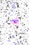 |
Fig. 1. Spectroscopically confirmed members in CARLA J09504+2743 and CARLA-Ser J09504+2743 and the X-ray counterpart emission contours corresponding to one to five times the background level (magenta contours). The blue and brown circles denote the positions of the spectroscopically confirmed members in CARLA J09504+2743 and CARLA-Ser J09504+2743, respectively, in the Spitzer IRAC1 image. The blue crosses show observed galaxies without detected emission lines and, hence, without a measured redshift. |
We measured the total flux of the X-ray counterpart as 6.77 ± 1.51 × 10⁻¹⁴ erg s−1 cm−2 in the 0.5 − 5 keV energy band in a circular aperture with a radius of 27 arcsec (220 kpc). The analysis of its 1D profile did not allow us to securely distinguish it from a point source given the small number of photons. At the same time, a Kolmogorov-Smirnov test of the observed 2D photon distribution showed that the data are consistent with a point-source distribution only at the confidence level of p = 0.0037, which confirmed that the X-ray source has an extended component in addition to the point source corresponding to the AGN. This test is more sensitive to the 2D distribution of the signal, for instance, to the differences in ellipticity. Further technical details about the analysis of the X-ray data are provided in Appendix B.
We discuss possible sources of the extended emission other than the ICM in Appendix C.3. We conclude that the observed X-ray source is likely a combination of the AGN and some extended component. A more precise analysis of the source shape requires deep high-resolution observations.
3. Results and discussion
3.1. Spectroscopic confirmation of CARLA J0950+2743, and the serendipitous discovery of a new cluster at z = 2.24
We extracted emission line fluxes using the optimal extraction method described in Horne (1986). We modeled the 2D profile for each individual emission line with a single 2D Gaussian using the LMFIT Python package4, and we divided it by the error frame. We then extracted fluxes and uncertainties using a 2D Gaussian weighting. Our measurements are shown in Fig. 2 and Table 1.
Spectroscopic measurements for confirmed cluster members in the CARLA J0950+2743 field.
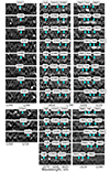 |
Fig. 2. Parts of the reduced coadded 2D MMIRS spectra for the eight spectroscopically confirmed cluster members in CARLA J0950+2743 at z = 2.363 ± 0.005 (top) and for five spectroscopically confirmed cluster members in CARLA-Ser J0950+2743 at z = 2.243 ± 0.008 (bottom). The cyan arrows indicate the positions of redshifted Hα+[NII], Hβ, [O III], and [OII] emission lines. The extracted 1D spectra are shown in Figure A.1. |
Following Noirot et al. (2018) and because our observed flux have similar flux depth that their observations, we spectroscopically confirmed CARLA J0950+2743 using the Eisenhardt et al. (2008) criteria for z > 1 clusters, which are that at least five galaxies must lie within ±2000(1 + z) km s−1 from the AGN redshift range within a physical radius of 2 Mpc. We identified eight galaxies that satisfied these criteria with Hα detections (S/N > 8), six of which also show other prominent emission lines. The shorter J/zJ setup integration time led to a lower S/N in the [OII] 3727Å detections, and these detections might also be affected by stronger dust extinction. We measured a cluster redshift of z = 2.363 ± 0.005 as the average of the redshifts of all spectroscopically confirmed members.
We also discovered a foreground structure at z = 2.243 ± 0.008 (155 Mpc comoving distance from CARLA J0950+2743), which is consistent with the Eisenhardt et al. (2008) criteria. This cluster, which we name CARLA-Ser J0950+2743 following Noirot et al. (2018), presents five galaxies with Hα emission and three galaxies that also show [OIII] emission (Fig. 2 and Table 1). Because only three galaxies show multiple emission lines, this confirmation and cluster classification should be validated with further observations. Following the CARLA cluster classification in Noirot et al. (2018), we classified these two structures as “probable clusters” because we do not observe a significant galaxy overdensity or high fractions of passive galaxies close to the spectroscopically confirmed members. Our spectroscopically confirmed galaxies are line emitters and star-forming galaxies.
3.2. Cluster mass constraints from X-ray data assuming a hot ICM
The estimated flux in the 0.5–5 keV (see Fig. 3) band corresponds to the observed luminosity of L0.5−5keV = 2.9 ± 0.6 × 1045 erg s−1. We denote with L0.5−5keV the X-ray luminosity in the 0.5–5 keV observed band, which corresponds to 1.7–17 keV restframe at z = 2.36.
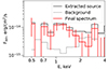 |
Fig. 3. X-ray spectrum extracted in an aperture with a radius of 27 arcsec, centered on the AGN (black), and the background spectrum (gray). The red line shows the spectrum of the source without the background. |
Because of the small number of detected photons and the correspondingly large error bars, the shape of the X-ray spectrum is consistent with a wide range of possible components, including a power-law component with Γ = 2, which is typical for AGNs, and all possible variations of ICM bremsstrahlung emission. We expect that the X-ray spectrum is likely to be a combination of these components. However, the limited depth of the dataset prevents us from decomposing the data more precisely. Hereafter, we choose a bremsstrahlung model to parameterize the X-ray spectral shape, but we verified that the choice of other models, or their combination, does not affect the results significantly. A pure bremsstrahlung model delivers the most conservative estimate of the k-correction range because for a power law with Γ = 2, the k-correction is 1.
To estimate the k-correction, we modeled the observed X-ray spectrum with XSPEC (Dorman & Arnaud 2001) using the model APEC, which corresponds to free-free transitions. This is a dominating emission regime in sparse hot plasma in galaxy clusters (Böhringer & Werner 2010). This modeling resulted in an electron temperature estimate of  keV. This temperature corresponds to a k-correction of kX = 0.612, which is needed to convert the observed flux into the restframe at z ∼ 2.2. Using the SHERPA tool (Doe et al. 2007), we estimate
  erg s−1 and LX = 4.5 ± 1.0 × 1045 erg s−15.
When we assumed a redshift of z = 2.363, the luminosity estimate corresponds to a total dark matter mass of  , according to the LX–M2500 relation (Connor et al. 2014). This considers the 1σ scatter in the relation, which is 0.1 dex (added to the systematic uncertainty). We also estimated the mass iteratively using two scaling relations: the M-T and the T-L relation. This allowed us to avoid uncertainties related to k-corrections because we did not need to estimate the k-correction from observations, but only from the temperature using the M-T scaling relation. This approach yielded M2500 = 0.80 ± 0.25 × 10¹⁴ M⊙, which is very close to the mass estimate that uses k-corrections.
For the transformations that were calibrated in the Magneticum cosmological hydrodynamic simulation (Ragagnin et al. 2021), we converted the measurement of M2500 into 
 . For a redshift z = 2.243, our mass estimate does not change significantly if the difference in the luminosity distances results in a luminosity ratio of 1.136. Based on the power-law index of the LX − M2500 relation of 0.305, the mass estimate would even be 8% lower.
We used  keV to estimate the k-correction. Its uncertainty therefore contributes to the systematic uncertainty of the mass estimate. For the 3σ lower limit of the temperature (TX = 2.50 keV), the k-correction is kX = 1.43, which yields M200 = 3.76 × 10¹⁴ M⊙. At the same time, the 3σ upper limit for TX of 35 keV is not physically possible because the highest values observed in galaxy clusters are about TX ∼ 10 keV, which yields kX = 0.414 and corresponds to M200 = 3.25 × 10¹⁴ M⊙.
Based on the statistical and systematic errors, which are independent, we conclude that if all the X-ray emission were due to an extended ICM emission, it would correspond to a total combined dark matter mass of 
 for the two clusters. Our observations do not permit us to confirm a thermal emission. We therefore discuss alternative explanations for the observed X-ray extended contribution in Appendix C.3.
We also take into account that at least part of the X-ray emission is due to the AGN. The total X-ray luminosity and the estimated AGN luminosity from multiwavelength data are consistent within ∼3σ (see Appendix C). This means that we cannot formally rule out that the X-ray flux is completely due to the AGN. However, if that were true, it would contradict our results from the KS test, which showed that the observed X-ray emission is not consistent with a single point source, and moreover, the X-ray emission is not centered on the AGN, but on a galaxy overdensity close to it.
Our best estimate of the AGN contribution based on the multiwavelength scaling relations of the X-ray surface brightness distribution is 32±22% (Appendix C.1), and our final total dark matter mass estimate is 
 . However, the scatter in the fraction of a possible AGN contribution does not affect the mass estimate strongly: In the very pessimistic case that a +2σ outlier results in an AGN contribution of 76%, the mass estimate would only change to
 .
.
The association of the X-ray counterpart with these two structures can also be secured by further spectroscopic observations that may deliver more complete galaxy catalogs. Based on these more complete catalogs, we may be able to exclude the existence of hypothetical low-redshift galaxy structures (or constrain them) that may contaminate the X-ray detection.
In general, additional observations will also help us to validate the dark matter mass estimate, which is higher by one order of magnitude than the estimate based on an abundance matching using the observed stellar mass within 1 arcmin from the peak of the X-ray emission (see Appendix D).
3.3. Perspectives of the cosmological implications
CARLA J0950+2743 and CARLA-Ser J0950+2743 and their X-ray counterpart can be used for future studies of the structure formation in the cosmological context. However, the interpretation of the X-ray observations of these clusters will be also affected by the superposition of these systems.
If the diffuse emission originates from the ICM in only one of these two clusters, its total luminosity can be used to set a lower limit on the cluster mass because the luminosity of a more massive cluster is always higher (or equal) than a half of the sum of the luminosities of two clusters.
The analysis of the Magneticum Pathfinder suite of cosmological simulations showed that the virial masses of clusters at z = 2.36 in case of the largest Box 0 (2688 Mpc h)−3 box size (Remus et al. 2023) do not exceed Mvir ≃ 3 × 10¹⁴ M⊙. This value is close to the total dark matter mass estimate for our two clusters derived from the X-ray analysis, when we convert M200 to Mvir following Ragagnin et al. 2021. We show the total virial mass of our two clusters in color in Fig. 4, considering different percentage levels of contamination from the AGN.
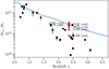 |
Fig. 4. Comparison of the mass estimate for CARLA J0950+2743 for different contamination levels from 0 to 99% (brown points), including the most realistic value of 32% (red point) with measurements for other structures (black points), compiled in Remus et al. (2023), which includes clusters from Shimasaku et al. (2003), Venemans et al. (2004), Ouchi et al. (2005), Toshikawa et al. (2012, 2014), Higuchi et al. (2019). Chanchaiworawit et al. (2019), Toshikawa et al. (2020), Calvi et al. (2021) and the virial mass of the most massive halo in the snapshots at different redshifts (blue line) for the Box 0 simulation set. |
Even under the assumption of an AGN X-ray contamination level of 90% (e.g., ≈2.5σ higher than the average contamination derived from scaling relations), it would still be one of the most massive clusters at its redshift if the X-ray thermal emission were dominated by one of the two clusters.
The implications of CARLA J0950+2743 and CARLA-Ser J0950+2743 in the cosmological context require deeper high-resolution X-ray observations to precisely constrain the contribution from AGN and a possible contamination from other point sources, such as those found in the field of some other high-redshift galaxy clusters and protoclusters, such as Spiderweb at z = 2.16 (Tozzi et al. 2022). Deeper and more complete spectroscopic observations are required as well.
4. Summary
Using deep ground-based NIR spectroscopy, we confirmed the CARLA J0950+2743 galaxy cluster at z = 2.363 ± 0.005 following the Eisenhardt et al. (2008) criteria. Specifically, we confirmed eight spectroscopic members within 2000 × (1 + z) km s−1 and a physical radius of 2 Mpc, including five galaxies with multiple emission lines.
We also serendipitously discovered another structure, CARLA-Ser J0950+2743 at z = 2.243 ± 0.008, which we classified as a cluster following the Eisenhardt et al. (2008) criteria. However, this last classification is based on five spectroscopically confirmed members, only three of which have multiple emission lines. This confirmation would benefit from deeper observations so that more galaxies with multiple emission lines might be observed, while the Eisenhardt et al. (2008) criteria would need at least five certain spectroscopically confirmed members.
Archival X-ray observations from the Chandra observatory revealed a counterpart that is consistent with a total dark matter halo mass of 
 for the two clusters, if the emission is associated with the cluster ICM and assuming an AGN contribution of ∼30%. We discuss in the appendix that the total mass estimate from an abundance matching is lower by an order of magnitude.
To improve each cluster mass estimate, deeper high-resolution X-ray observations are needed to better constrain the AGN contribution to the signal. At the same time, submillimeter observations of the Sunyaev–Zel’dovich effect (Sunyaev & Zeldovich 1972) may not be efficient for our source given the effective mass limit of submillimeter surveys, which depends on their depth and angular resolution (Bleem et al. 2020) and the presence of the AGN.
Further spectroscopic observations are needed to secure the association of the X-ray source with these two structures at z > 2.0 and to exclude or constrain possible contamination (see Appendix D).
CARLA J0950+2743 and CARLA-Ser J0950+2743 provide a unique opportunity to study the formation of the large-scale structure of the Universe at the age of 2–3 billion years after the Big Bang, as well as the evolution of the galaxy population in dense environments and the main factors driving it.
Infrared Array Camera, (IRAC, Fazio et al. 2004).
Hereafter, we denote the bolometric luminosity with LX, following Connor et al. (2014).
We can consider this bin size optimal because it yields S/N> 3 in most bins in the area of the detection and it does not yet affect much the spatial information.
Acknowledgments
We thank Université Paris Cité, which funded KG’s Ph.D. research. We also thank Franz Bauer and Alexei Vikhlinin for useful discussions. KG thanks Victoria Toptun for the fruitful discussions related to the X-ray analysis. IC’s research is supported by the Telescope Data Center, Smithsonian Astrophysical Observatory. Observations reported here were obtained at the MMT Observatory, a joint facility of the Smithsonian Institution and the University of Arizona. We gratefully acknowledge support from the CNRS/IN2P3 Computing Center (Lyon - France) for providing computing and data-processing resources needed for this work. This work was supported by CNES, focused on the Euclid space mission, and by the CNRS/IN2P3.
References
- Abazajian, K. N., Adelman-McCarthy, J. K., Agüeros, M. A., et al. 2009, ApJS, 182, 543 [Google Scholar]
- Abazajian, K. N., Adshead, P., Ahmed, Z., et al. 2016, arXiv e-prints [arXiv:1610.02743] [Google Scholar]
- Afanasiev, A. V., Mei, S., Fu, H., et al. 2023, A&A, 670, A95 [NASA ADS] [CrossRef] [EDP Sciences] [Google Scholar]
- Ahumada, R., Allende Prieto, C., Almeida, A., et al. 2020, ApJS, 249, 3 [NASA ADS] [CrossRef] [Google Scholar]
- Ascaso, B., Mei, S., & Benítez, N. 2015, MNRAS, 453, 2515 [Google Scholar]
- Bariuan, L. G. C., Snios, B., Sobolewska, M., Siemiginowska, A., & Schwartz, D. A. 2022, MNRAS, 513, 4673 [NASA ADS] [CrossRef] [Google Scholar]
- Bertin, E., & Arnouts, S. 1996, A&AS, 117, 393 [NASA ADS] [CrossRef] [EDP Sciences] [Google Scholar]
- Bleem, L. E., Bocquet, S., Stalder, B., et al. 2020, ApJS, 247, 25 [Google Scholar]
- Böhringer, H., & Werner, N. 2010, A&ARv, 18, 127 [Google Scholar]
- Calvi, R., Dannerbauer, H., Arrabal Haro, P., et al. 2021, MNRAS, 502, 4558 [NASA ADS] [CrossRef] [Google Scholar]
- Capak, P. L., Riechers, D., Scoville, N. Z., et al. 2011, Nature, 470, 233 [Google Scholar]
- Casey, C. M., Cooray, A., Capak, P., et al. 2015, ApJ, 808, L33 [NASA ADS] [CrossRef] [Google Scholar]
- Chanchaiworawit, K., Guzmán, R., Salvador-Solé, E., et al. 2019, ApJ, 877, 51 [NASA ADS] [CrossRef] [Google Scholar]
- Chilingarian, I., Beletsky, Y., Moran, S., et al. 2015, PASP, 127, 406 [CrossRef] [Google Scholar]
- Connor, T., Donahue, M., Sun, M., et al. 2014, ApJ, 794, 48 [NASA ADS] [CrossRef] [Google Scholar]
- Cooke, E. A., Hatch, N. A., Rettura, A., et al. 2015, MNRAS, 452, 2318 [NASA ADS] [CrossRef] [Google Scholar]
- Darvish, B., Scoville, N. Z., Martin, C., et al. 2020, ApJ, 892, 8 [NASA ADS] [CrossRef] [Google Scholar]
- Davis, J. E., Bautz, M. W., Dewey, D., et al. 2012, SPIE Conf. Ser., 8443, 84431A [NASA ADS] [Google Scholar]
- Diener, C., Lilly, S. J., Ledoux, C., et al. 2015, ApJ, 802, 31 [NASA ADS] [CrossRef] [Google Scholar]
- Doe, S., Nguyen, D., Stawarz, C., et al. 2007, ASP Conf. Ser., 376, 543 [NASA ADS] [Google Scholar]
- Dorman, B., & Arnaud, K. A. 2001, ASP Conf. Ser., 238, 415 [NASA ADS] [Google Scholar]
- Dye, S., Lawrence, A., Read, M. A., et al. 2018, MNRAS, 473, 5113 [Google Scholar]
- Eifler, T., Miyatake, H., Krause, E., et al. 2021, MNRAS, 507, 1746 [NASA ADS] [CrossRef] [Google Scholar]
- Eisenhardt, P. R. M., Brodwin, M., Gonzalez, A. H., et al. 2008, ApJ, 684, 905 [Google Scholar]
- Erlund, M. C., Fabian, A. C., Blundell, K. M., Celotti, A., & Crawford, C. S. 2006, MNRAS, 371, 29 [Google Scholar]
- Fasano, G., & Franceschini, A. 1987, MNRAS, 225, 155 [NASA ADS] [CrossRef] [Google Scholar]
- Fazio, G. G., Hora, J. L., Allen, L. E., et al. 2004, ApJS, 154, 10 [Google Scholar]
- Gandhi, P., Horst, H., Smette, A., et al. 2009, A&A, 502, 457 [NASA ADS] [CrossRef] [EDP Sciences] [Google Scholar]
- Ghirardini, V., Bulbul, E., Artis, E., et al. 2024, A&A, 689, A298 [NASA ADS] [CrossRef] [EDP Sciences] [Google Scholar]
- Gobat, R., Daddi, E., Onodera, M., et al. 2011, A&A, 526, A133 [NASA ADS] [CrossRef] [EDP Sciences] [Google Scholar]
- Grishin, K. A., Chilingarian, I. V., Afanasiev, A. V., et al. 2021, Nat. Astron., 5, 1308 [NASA ADS] [CrossRef] [Google Scholar]
- Harris, D. E., & Grindlay, J. E. 1979, MNRAS, 188, 25 [NASA ADS] [Google Scholar]
- Higuchi, R., Ouchi, M., Ono, Y., et al. 2019, ApJ, 879, 28 [Google Scholar]
- Horne, K. 1986, PASP, 98, 609 [Google Scholar]
- Just, D. W., Brandt, W. N., Shemmer, O., et al. 2007, ApJ, 665, 1004 [Google Scholar]
- Kahn, S. 2018, in 42nd COSPAR Scientific Assembly, 42, E1.16-5-18 [Google Scholar]
- Kakimoto, T., Tanaka, M., Onodera, M., et al. 2024, ApJ, 963, 49 [NASA ADS] [CrossRef] [Google Scholar]
- Kelson, D. D. 2003, PASP, 115, 688 [NASA ADS] [CrossRef] [Google Scholar]
- Khadka, N., Zajaček, M., Prince, R., et al. 2023, MNRAS, 522, 1247 [NASA ADS] [CrossRef] [Google Scholar]
- Kimmig, L. C., Remus, R. S., Seidel, B., et al. 2023, arXiv e-prints [arXiv:2310.16085] [Google Scholar]
- Kolmogorov, A. 1933, G. Ist. Ital. Attuari, 4, 83 [Google Scholar]
- Koyama, Y., Polletta, M. d. C., Tanaka, I., et al. 2021, MNRAS, 503, L1 [NASA ADS] [CrossRef] [Google Scholar]
- Kozłowski, S. 2017, ApJS, 228, 9 [CrossRef] [Google Scholar]
- Lanzuisi, G., Piconcelli, E., Fiore, F., et al. 2009, A&A, 498, 67 [NASA ADS] [CrossRef] [EDP Sciences] [Google Scholar]
- Laporte, N., Zitrin, A., Dole, H., et al. 2022, A&A, 667, L3 [NASA ADS] [CrossRef] [EDP Sciences] [Google Scholar]
- Laureijs, R., Amiaux, J., Arduini, S., et al. 2011, arXiv e-prints [arXiv:1110.3193] [Google Scholar]
- Lee, K.-G., Hennawi, J. F., White, M., et al. 2016, ApJ, 817, 160 [NASA ADS] [CrossRef] [Google Scholar]
- Lemaux, B. C., Le Fèvre, O., Cucciati, O., et al. 2018, A&A, 615, A77 [NASA ADS] [CrossRef] [EDP Sciences] [Google Scholar]
- Lusso, E., Comastri, A., Vignali, C., et al. 2010, A&A, 512, A34 [NASA ADS] [CrossRef] [EDP Sciences] [Google Scholar]
- Lutz, D., Maiolino, R., Spoon, H. W. W., & Moorwood, A. F. M. 2004, A&A, 418, 465 [NASA ADS] [CrossRef] [EDP Sciences] [Google Scholar]
- MacLeod, C. L., Ivezić, Ž., Sesar, B., et al. 2012, ApJ, 753, 106 [NASA ADS] [CrossRef] [Google Scholar]
- McConachie, I., Wilson, G., Forrest, B., et al. 2022, ApJ, 926, 37 [NASA ADS] [CrossRef] [Google Scholar]
- McLeod, B., Fabricant, D., Nystrom, G., et al. 2012, PASP, 124, 1318 [NASA ADS] [CrossRef] [Google Scholar]
- Mei, S., Hatch, N. A., Amodeo, S., et al. 2023, A&A, 670, A58 [NASA ADS] [CrossRef] [EDP Sciences] [Google Scholar]
- Merloni, A., Heinz, S., & di Matteo, T. 2003, MNRAS, 345, 1057 [Google Scholar]
- Morishita, T., Roberts-Borsani, G., Treu, T., et al. 2023, ApJ, 947, L24 [NASA ADS] [CrossRef] [Google Scholar]
- Muzzin, A., van der Burg, R. F. J., McGee, S. L., et al. 2014, ApJ, 796, 65 [Google Scholar]
- Noirot, G., Stern, D., Mei, S., et al. 2018, ApJ, 859, 38 [NASA ADS] [CrossRef] [Google Scholar]
- Oke, J. B., & Gunn, J. E. 1983, ApJ, 266, 713 [NASA ADS] [CrossRef] [Google Scholar]
- Ouchi, M., Shimasaku, K., Akiyama, M., et al. 2005, ApJ, 620, L1 [NASA ADS] [CrossRef] [Google Scholar]
- Overzier, R. A., Harris, D. E., Carilli, C. L., et al. 2005, A&A, 433, 87 [NASA ADS] [CrossRef] [EDP Sciences] [Google Scholar]
- Pavesi, R., Riechers, D. A., Sharon, C. E., et al. 2018, ApJ, 861, 43 [Google Scholar]
- Peacock, J. A. 1983, MNRAS, 202, 615 [NASA ADS] [Google Scholar]
- Press, W. H., Teukolsky, S. A., Vetterling, W. T., & Flannery, B. P. 2002, Numerical Recipes in C++: The Art of Scientific Computing (William H: Press) [Google Scholar]
- Ragagnin, A., Saro, A., Singh, P., & Dolag, K. 2021, MNRAS, 500, 5056 [Google Scholar]
- Remus, R.-S., Dolag, K., & Dannerbauer, H. 2023, ApJ, 950, 191 [NASA ADS] [CrossRef] [Google Scholar]
- Saez, C., Brandt, W. N., Shemmer, O., et al. 2011, ApJ, 738, 53 [Google Scholar]
- Sambruna, R. M., Eracleous, M., & Mushotzky, R. F. 1999, ApJ, 526, 60 [NASA ADS] [CrossRef] [Google Scholar]
- Santos, J. S., Fassbender, R., Nastasi, A., et al. 2011, A&A, 531, L15 [NASA ADS] [CrossRef] [EDP Sciences] [Google Scholar]
- Shimasaku, K., Ouchi, M., Okamura, S., et al. 2003, ApJ, 586, L111 [NASA ADS] [CrossRef] [Google Scholar]
- Smirnov, N. 1948, Ann. Math. Stat., 19, 279 [CrossRef] [Google Scholar]
- Spitler, L. R., Labbé, I., Glazebrook, K., et al. 2012, ApJ, 748, L21 [NASA ADS] [CrossRef] [Google Scholar]
- Stern, D. 2015, ApJ, 807, 129 [Google Scholar]
- Strazzullo, V., Coogan, R. T., Daddi, E., et al. 2018, ApJ, 862, 64 [NASA ADS] [CrossRef] [Google Scholar]
- Strazzullo, V., Pannella, M., Mohr, J. J., et al. 2019, A&A, 622, A117 [NASA ADS] [CrossRef] [EDP Sciences] [Google Scholar]
- Sunyaev, R. A., & Zeldovich, Y. B. 1972, Comm. Astrophys. Space Phys., 4, 173 [Google Scholar]
- Tanaka, M., Onodera, M., Shimakawa, R., et al. 2024, ApJ, 970, 59 [Google Scholar]
- Toptun, V. A., Chilingarian, I. V., Grishin, K. A., & Katkov, I. Y. 2023, PASP, 135, 084102 [Google Scholar]
- Toshikawa, J., Kashikawa, N., Ota, K., et al. 2012, ApJ, 750, 137 [Google Scholar]
- Toshikawa, J., Kashikawa, N., Overzier, R., et al. 2014, ApJ, 792, 15 [NASA ADS] [CrossRef] [Google Scholar]
- Toshikawa, J., Malkan, M. A., Kashikawa, N., et al. 2020, ApJ, 888, 89 [Google Scholar]
- Toshikawa, J., Wuyts, S., Kashikawa, N., et al. 2024, arXiv e-prints [arXiv:2404.15910] [Google Scholar]
- Tozzi, P., Pentericci, L., Gilli, R., et al. 2022, A&A, 662, A54 [NASA ADS] [CrossRef] [EDP Sciences] [Google Scholar]
- Venemans, B. P., Röttgering, H. J. A., Overzier, R. A., et al. 2004, A&A, 424, L17 [NASA ADS] [CrossRef] [EDP Sciences] [Google Scholar]
- Vikhlinin, A., Burenin, R. A., Ebeling, H., et al. 2009, ApJ, 692, 1033 [Google Scholar]
- Vollmer, B., Gassmann, B., Derrière, S., et al. 2010, A&A, 511, A53 [NASA ADS] [CrossRef] [EDP Sciences] [Google Scholar]
- Wang, T., Elbaz, D., Daddi, E., et al. 2016, ApJ, 828, 56 [NASA ADS] [CrossRef] [Google Scholar]
- Wang, G. C. P., Hill, R., Chapman, S. C., et al. 2021, MNRAS, 508, 3754 [NASA ADS] [CrossRef] [Google Scholar]
- Wylezalek, D., Galametz, A., Stern, D., et al. 2013, ApJ, 769, 79 [NASA ADS] [CrossRef] [Google Scholar]
- Wylezalek, D., Vernet, J., De Breuck, C., et al. 2014, ApJ, 786, 17 [NASA ADS] [CrossRef] [Google Scholar]
- Yonekura, N., Kajisawa, M., Hamaguchi, E., Mawatari, K., & Yamada, T. 2022, ApJ, 930, 102 [NASA ADS] [CrossRef] [Google Scholar]
- Yuan, T., Nanayakkara, T., Kacprzak, G. G., et al. 2014, ApJ, 795, L20 [NASA ADS] [CrossRef] [Google Scholar]
- Zheng, W., Shu, X., Moustakas, J., et al. 2014, ApJ, 795, 93 [NASA ADS] [CrossRef] [Google Scholar]
- Zhou, L., Wang, T., Daddi, E., et al. 2024, A&A, 684, A196 [NASA ADS] [CrossRef] [EDP Sciences] [Google Scholar]
Appendix A: Spectroscopic observations and data reduction
For the MMIRS observations, we used a 4-position dithering pattern (ABA’B’) at +1.4, −1.0, +1.0, −1.4 arcsec. The individual exposure times were set to 300 sec. with the 4.426 sec. up-the-ramp nondestructive readout sequence using the 0.95 e-/ADU inverse gain. The readout noise per readout ∼15 e- was reduced to the effective value of ∼3 e- after 69 readouts.
We reduced data with the MMIRS pipeline (Chilingarian et al. 2015), which included the following steps: (i) reference pixel correction and up-the-ramp fitting of raw readouts; (ii) dark subtraction; (iii) flat fielding; (iv) extraction of 2D slitlets; (v) wavelength solution using OH lines; (vi) sky background subtraction using a modified Kelson (2003) technique with a global sky model; (vii) correction for the telluric absorption and relative flux calibration using observations of a A0V telluric standard star. We ran the pipeline on individual A−B (or A’−B’) dithered pairs.
We then co-added the dithered pairs from observations collected during different nights applying the weights inversely proportional to the squared seeing FWHM.
Finally, we performed the absolute flux calibration by using secondary calibration stars included in the masks by re-normalizing their fluxes to the H and Ks-band measurements from the UKIRT Hemisphere Survey (UHS Dye et al. 2018). Being a secondary flux calibration standard catalog, the UKIDSS/UHS does not show significant systematic effects either for stars or for galaxies (Toptun et al. 2023). Hence, we do not expect to have substantial (> 10%) flux calibration bias in our measurements.
Our datasets reach a 3σ sensitivity at 1.1 × 10⁻¹⁷ erg s−1 cm−2 and 1.4 × 10⁻¹⁷ erg s−1 cm−2, for mask1 and mask2, respectively, for a typical Hα emission line, with the restframe full width at half maximum of 9.7 Å. This corresponds to 1.2 × 10⁻¹⁸ erg s−1 cm−2 Å−1 and 1.5 × 10⁻¹⁸ erg s−1 cm−2 Å−1, for mask1 and mask2, respectively, in the continuum averaged between Hα and [SII].
For mask1, the achieved depth in J/zJ reached 1.6 × 10⁻¹⁷ erg s−1 cm−2 for the [OII] emission line, and 1.8 × 10⁻¹⁸ erg s−1 cm−2 Å−1 for the continuum in the region of this emission line.
In Fig. A.1, we show the 1D profiles for the spectroscopically confirmed members in CARLA J0950+2743 and CARLA-Ser J0950+2743 that were optimally extracted (Horne 1986) using Gaussian profile with FWHM = 0.74 arcsec. (3.7 pixels). Emission line detections on 1D profiles have systematically less S/N than in 2D datasets given that the flux extraction on the latter allows to take into account a full information about line profile.
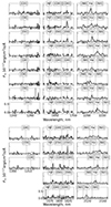 |
Fig. A.1. Parts of reduced co-added extracted 1D MMIRS spectra for the eight CARLA J0950+2743 (top) and the five CARLA-Ser J0950+2743 (bottom) spectroscopically confirmed cluster members. Dashed vertical lines indicate the positions of redshifted Hα+[NII], Hβ, [OIII], and [OII] emission lines. |
Appendix B: Spatial extent of an X-ray counterpart
We measured the flux of the X-ray cluster counterpart in the following way: (i) We selected a subsample of the registered events within a radius of 27 arcsec from the peak of the counts in the binned dataset, which identify our target; (ii) To estimate the background, we selected a subsample of events in two circular areas with radii 86 and 62 arcsec, in the same detector, but far enough from the extraction region of the main source; (iii) We then calculated the energy spectra of these three photon subsamples; (iv) We subtracted the background from the target spectrum, after renormalizing by the area covered by the regions; (v) We corrected the spectra taking into account the photon energy and effective area. We obtained a total target flux of 6.77 ± 1.51 × 10⁻¹⁴ erg s−1 cm−2 in the 0.5 − 5 keV energy band in the circular aperture with a radius of 27 arcsec (220 kpc).
Using the CHART web-tool6 we ran a raytrace simulation for the position of the AGN on the archival Chandra dataset for 1000 rays for a source with a spectral shape obtained from the modeling with XSPEC as discussed in Section 3.2. The obtained ray map was then reprojected on the detector plane using MARX (Davis et al. 2012) to obtain a model of the Chandra Point Spread Function (PSF).
To assess whether the distribution of detected photons corresponds to what is expected for a point source, we performed a Kolmogorov–Smirnov test (KS-test) (Kolmogorov 1933; Smirnov 1948). For this test, we estimated a 2D distribution of detected photons that contains two components: background and a point source. To estimate the contribution of each component, we spatially binned the observed photon events within a square window with the side of 600 pixels and the bin size of 32 pixels. We then modeled the derived 2D distribution by a linear combination of a constant component (background) and a PSF model. Inferred coefficients were used to assign background and point source the same flux amplitude as in the Chandra dataset. We use a classical two-sample KS test (Peacock 1983; Fasano & Franceschini 1987; Press et al. 2002), which provides a better ability of separating two distributions.
Using the 2DKS Python package7, we ran a KS test for the observed distribution of detected photons and 500 realizations of the model distribution. The median value of the KS-statistic D (the maximum deviation between the observed cumulative distribution function of the sample and the cumulative distribution function of the model distribution) is D = 0.0642, with a median value of the significance level to follow the same distribution of p = 0.0037 (see Fig. B.1).
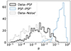 |
Fig. B.1. The distribution of the significance levels (p) for different realizations of the mock event lists obtained using the KS test for the observed distribution vs a point source distribution (black). As an additional test, we present the distribution of p for the cross-tested generated samples of event lists that correspond to point-source (blue) and for the tested background-only photon distribution (grey). |
As an additional cross-validation, we ran the same KS test for independently generated mock event lists that follow the model distribution. This test yielded a median D = 0.0362 and p = 0.27. At the same time to confirm the source detection, we also did a similar test between observed photon distribution and a pure background distribution what yielded a median D = 0.0735 and p = 0.00054, which securely confirms the presence of a source. From these results we conclude that: (i) Using a two-sample KS test for the Chandra dataset we can separate with high confidence a case of a pure point-source from a combination of a point source and extended one; (ii) The significance level that the observed photon distribution is drawn from a point-source distribution is p = 0.0037.
In Figures B.2 and B.3, we show the radial profiles of the cluster counterpart in X-ray obtained with 55 photons and a generated PSF model. In Figure B.2 and B.3 we provide the 1D profile for the source and for PSF model extracted in circular and elliptical (b/a = 0.75) annuli respectively, both centered on the position of the AGN. The profile derived with elliptical annuli is normalized to the total number of photons, while normalization of the coefficients for the profile in circular annuli is obtained by using a χ2 minimization.
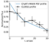 |
Fig. B.2. Radial profile of detected photons extracted from the Chandra dataset in circular annuli centered on the CARLA J0950+2743 AGN (black), compared to the PSF profile modeled using ChaRT+MARX (blue) with the normalization factor derived from the χ2 minimization. |
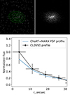 |
Fig. B.3. Upper panel: Chandra image of CARLA J0950+2743 (left) and simulated PSF (right) with overlapped the elliptical annuli used for the 1D signal profile (in green). All regions are centered on the AGN. Lower panel: Radial profile of the detected photons per unit area in the Chandra dataset centering on the CARLA J0950+2743 AGN, compared to the simulated Chandra PSF radial profile (in black). Both profiles are normalized to the total number of net counts found in the extraction regions (see upper panel). |
The two 1D profile analyses are consistent with emission from a point source, but the extended emission detected from our spatial analysis is also consistent with these profiles, given the large uncertainties on the data.
The spatial distribution of our source is also substantially rounder (b/a = 0.80±0.16) than the PSF (b/a = 0.5) at that position in the Chandra FoV (Fig. C.1), and this could explain why our spatial analysis and KS test are more conclusive to show evidence for an extended source component.
The error bars clearly demonstrate that our modeling of the observed photon distribution is limited by the statistical effects, i.e. number of detected photons, rather than the PSF systematics.
Appendix C: Estimates of the AGN contribution to X-ray luminosity
C.1. Estimates of the AGN X-ray luminosity
The only available archival Chandra X-ray dataset does not provide a precise measurement of the AGN contribution, therefore we use several multiwavelength scaling relations to estimate it. Each of these relations has a relatively high intrinsic spread, however, because they probe different physical regions and/or mechanisms of an AGN, together they provide a very good constraint of the flux.
By combining the estimates obtained using relations between AGN luminosities in the X-ray and UV or IR, we estimate a possible AGN contribution as  , taking the average of all contributions estimated in the following subsection, excluding the estimate obtained from the Fundamental Plane of the black hole activity, for which we cannot conclude with reasonable uncertainties. For the uncertainties, we took into account the scatter of the scaling relations, the measurements of the X-ray source flux, and the uncertainty on the variables used in the scaling relations. The details of our estimations are given in the subsections below.
C.1.1. Fundamental Plane of the black hole activity.
The fundamental plane of black hole activity (Merloni et al. 2003) relates the black hole mass, the radio luminosity at 5 GHz, and the X-ray luminosity in the 2–10 keV range. It suggests that the processes governing black hole accretion and jet emission are scalable and can be described by universal laws for black holes in the mass ranges from stellar to supermassive. A recent re-calibration of the fundamental plane of black hole activity based on observational data for intermediate-redshift quasars (Bariuan et al. 2022) has a scatter of ∼0.62 dex for radio-loud AGN, which is smaller than that of the original relation (Merloni et al. 2003, ∼0.8-0.9 dex). But it still leads to 1σ uncertainties of a factor of ∼3 in X-ray luminosity. The black hole mass estimate for the AGN from the broad lines (CIV]) is MBH = 2.0 − 2.6 × 10⁹ M⊙ (MacLeod et al. 2012; Kozłowski 2017) and the radio continuum luminosity νFν = 2.9 × 1044ergs−1 estimated from Vollmer et al. (2010) yields the AGN X-ray luminosity of  , which substantially exceeds the X-ray luminosity that we measured for our source. However, given the large scatter, we cannot consider this estimate for assessing the AGN contribution, but can only conclude that it can be between 20% and 100% within the 3σ range.
C.1.2. L0.2 − 2keV − L6μm relation.
The relation between the AGN luminosity in the X-ray and in the infrared (IR) reflects the tight dependence of the emission of the hot corona and the emission from the accretion disk irradiated by the dust (Lutz et al. 2004; Gandhi et al. 2009; Lanzuisi et al. 2009). We use the correlation between the mid-IR flux at 6 μm (Stern 2015) and X-ray that relates the X-ray emission to the emission of the warm dust in the AGN torus, and is less affected by the intrinsic dust attenuation unlike the correlations based on the UV luminosity. Using the WISE W4 magnitude measurement for the AGN that perfectly matches the restframe 6 μm, we estimated L0.5 − 5keV = 0.75 × 1045 erg s−1, or ∼25% of the total observed X-ray luminosity.
The scatter, estimated for the "filtered high-luminosity quasar" sample from Just et al. (2007), used to build the regression fit in Stern (2015) is 0.26 dex. Adding the uncertainty of the W4 magnitude measurement, this leads to the final estimate of  erg s−1. This corresponds to an AGN contribution of
  .
.
C.1.3. L2keV − LNUV correlation.
We use the empirical correlation between the AGN luminosity in soft X-ray and the near-UV from Lusso et al. (2010) with an intrinsic scatter of 0.35 dex. It relates the accretion disk luminosity in the continuum at 2500Å to the X-ray generated by the corona.
From available SDSS spectra, at λ = 8400 Å, we can directly measure the UV restframe continuum flux as F2500A = 3 × 10⁻¹⁷ erg s−1 cm2 Å−1 that corresponds to the UV restframe luminosity density of Lν, 2500A = 1.10 × 1031 erg s−1 cm2 Hz−1.
From this, we derive the X-ray luminosity spectral density L2keV = 5.1 × 1026 erg s−1 cm2 Hz−1 (Khadka et al. 2023). The uncertainty on F2500A is less than 5%, so it does not affect the uncertainty of L2keV estimate.
Using the CALC_KCORR procedure in the Chandra SHERPA toolkit, we converted the L2keV to the observed X-ray luminosity in the 0.5 − 5 keV bandpass and obtain L0.5 − 5keV = 1.1 × 1045 erg s−1 assuming Γ = 1.4 for RL AGN (Sambruna et al. 1999; Saez et al. 2011). Adding the scatter of the LX − L2500Å correlation of 0.35 dex, we obtain  erg s−1. This corresponds to an AGN contribution of
  .
.
C.2. AGN contribution from the decomposition of the X-ray photon distribution
To directly constrain a contribution from the AGN point source in X-ray, we performed a decomposition of the observed background subtracted distribution of detected X-ray photons by representing it with a linear combination of a point-source component used in Section 2.3, and an extended Gaussian distribution, both convolved with a PSF (Fig. C.1). For a bin size of 18 × 18 pixels (9 arcsec)8, the recovered contribution of the point source is 35±26%.
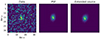 |
Fig. C.1. Decomposition of a binned Chandra X-ray event list for CARLA J0950+2743. Left: A binned event list with higher energy cut of 7keV; Middle: A binned event list for the point source; Right: A binned 2-D Gaussian model convolved with the Chandra PSF for the extended component. |
Given that the shape of the point source component is fixed while the shape of the diffuse emission is flexible, the estimated AGN fraction can be treated as an upper limit of AGN fraction in the observed X-ray luminosity.
C.3. Extended X-ray emission from inverse Compton scattering on a radio jet
The observed X-ray counterpart can be explained by sources other than the ICM. For example, deep high-resolution Chandra X-ray imaging of the Spiderweb protocluster revealed a population of point sources (AGN) (Tozzi et al. 2022) that would be interpreted as extended ICM emission in case of lower angular resolution, similar to the Chandra dataset for our cluster.
The inverse Compton (IC) scattering of the CMB photons on the electrons in the AGN jet can produce substantial X-ray emission (Harris & Grindlay 1979). To estimate the possibility of high contribution of possible IC from the AGN to the observed X-ray luminosity, we followed an approach similar to that used for the cluster J1001+02 at z = 2.51 (Wang et al. 2016), assuming that all the observed radio and X-ray emission originates from the AGN.
Our calculations yield a magnetic field estimate of ∼0.5μG, which is almost an order of a magnitude smaller than typical magnetic fields in the systems where the IC is observed (Overzier et al. 2005). We therefore conclude that the observed extended X-ray emission is unlikely to be produced by IC scattering.
The observed X-ray flux can also emerge from the IC structures in the radio-lobes (Erlund et al. 2006), but observed X-ray luminosities of these objects are of the order of a few times of 1044 erg/s, substantially lower than expected luminosity of the diffuse emission. However, the very existence of lobe may already serve as a indirect confirmation of the ICM.
Appendix D: Galaxy overdensities around the peak of the X-ray emission
The CARLA J0950+2743 field has a galaxy density of 18.8 arcmin−2 (> 4.4σ with respect to the field; Wylezalek et al. (2013, 2014)). However, when compared to the other CARLA spectroscopically confirmed clusters at z∼2 (Mei et al. 2023), the signal-to-noise ratio (S/N) of the overdensities of galaxies with IRAC1-IRAC2 > -0.1 (Fig. D.1) never reaches S/N ≳ 13, and never S/N ≳ 10 around the peak of the X-ray emission and the position of the AGN (see Fig. D.1). The other CARLA clusters at z ∼ 2 instead show galaxy overdensities with S/N > 17 up to z ∼ 2.8 (with two with overdensities of S/N ∼ 25 and 30) around the AGN and large percentages of passive galaxies, with a much more compact galaxy distribution (Mei et al. 2023). This seems to point to a large contribution to the total galaxy density calculated by Wylezalek et al. (2013, 2014) from two S/N ∼ 13 overdensities at ∼1.5 arcmin from the AGN, the spectroscopically confirmed members of the two confirmed clusters in this paper, and the X-ray emission peak. Both show high numbers of galaxies with colors compatible with z < 2, following Cooke et al. (2015).
The estimated total dark matter masses of the other CARLA spectroscopically confirmed clusters at z ∼ 2 are in the range 4 × 10¹³ M⊙ < Mh < 2 × 10¹⁴ M⊙. The only clusters with total dark matter mass estimated to be close to the combined mass estimated for this paper are CARLA J1018+0530 and CARLA J0800+4029, with an estimated Mh ∼ 2 × 10¹⁴ M⊙. One shows a very concentrated overdensity with S/N > 30 around the AGN, and the other three overdensities with S/N ∼ 16 that encircle the AGN. This is puzzling, because we do not observe any high S/N galaxy overdensity around the CARLA J0950+2743 AGN and the peak of the X-ray emission.
For these reasons, we also explore another hypothesis. The extended X-ray emission might also be due to a lower redshift structure on the line of sight of our two clusters. In Fig. D.2, we show the positions of galaxies with colors and magnitudes compatible with being z∼1.2-1.5, from the color-magnitude diagram in the (i−IRAC1) vs IRAC1 color–magnitude diagram following Cooke et al. (2015).
From the positions of these galaxies, we cannot exclude that the extended X-ray emission is due to a lower redshift structure. If the X-ray extended emission is due to this structure, its mass would be 
 ×1014 M⊙, after subtracting the same AGN contribution of ∼ 30% used for the final estimate of the combined total dark matter mass of the two z∼2 clusters in this paper.
We also observe that galaxies with colors and magnitudes compatible to have redshift z< 2 show high concentrations at the position of the highest galaxy overdensities of galaxies with IRAC1-IRAC2>-0.1, confirming again that there are not high S/N overdensities of galaxies with z> 2 around the AGN or the peak of the X-ray emission.
Following Mei et al. (2023), we convert the IRAC1 magnitudes in stellar mass estimates for all galaxies with IRAC1-IRAC2>-0.1 within 1 arcmin. of the position of the X-ray emission peak. These are galaxies belonging to the overdensity closer on the X-ray emission peak and the closer overdensity on the top right of it in Fig. D.1. We then calculate the total dark matter halo masses of these two overdensities from the obtained stellar mass, and obtain Mh ∼ 2 × 10¹² M⊙ and Mh ∼ 3 × 10¹² M⊙ for the overdensity closest to the X-ray emission peak and Mh ∼ 6 × 10¹² M⊙ and Mh ∼ 2 × 10¹³ M⊙ for the other, at z ∼ 1.3 − 1.5 and z ∼ 2.2 − 2.3, respectively.
All these total dark matter estimates are about one order to two order of magnitude less than the combined total dark matter mass for our two clusters, as obtained from the X-ray emission, even when we correct for a AGN contribution of 75%. The different estimates can be consistent only if the AGN contribution to the X-ray emission is more than 75%, and dominates most of the X-ray emission, and even then we cannot conclude much about the redshift of the two galaxy overdensities within 1 arcmin from the peak of the X-ray emission.
In a similar way as the hypothesis that most of the X-ray emission is due to the AGN, only a dedicated spectroscopic campaign and deep X-ray observations that would identify more precisely the AGN contribution would be able to test this hypothesis and the consistency of our total dark matter mass estimates.
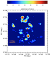 |
Fig. D.1. S/N of overdensity of galaxies with IRAC1-IRAC2>-0.1 in the CARLA J0950+2743 field. The red star shows the position of the peak of the X-ray emission. |
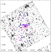 |
Fig. D.2. The Spitzer IRAC1 image with superposed X-ray contours and the positions of galaxies with colors and magnitudes compatible with structures at z∼1.2-1.5 (magenta crosses), from the color-magnitude diagram in the (i−IRAC1) vs IRAC1 color–magnitude diagram following Cooke et al. (2015). Blue and brown circles are spectroscopically confirmed members at z = 2.36 and z = 2.24 respectively, blue crosses are MMT spectroscopically followed-up galaxies without measured redshifts. |
All Tables
Spectroscopic measurements for confirmed cluster members in the CARLA J0950+2743 field.
All Figures
|
Fig. 1. Spectroscopically confirmed members in CARLA J09504+2743 and CARLA-Ser J09504+2743 and the X-ray counterpart emission contours corresponding to one to five times the background level (magenta contours). The blue and brown circles denote the positions of the spectroscopically confirmed members in CARLA J09504+2743 and CARLA-Ser J09504+2743, respectively, in the Spitzer IRAC1 image. The blue crosses show observed galaxies without detected emission lines and, hence, without a measured redshift. |
| In the text | |
|
Fig. 2. Parts of the reduced coadded 2D MMIRS spectra for the eight spectroscopically confirmed cluster members in CARLA J0950+2743 at z = 2.363 ± 0.005 (top) and for five spectroscopically confirmed cluster members in CARLA-Ser J0950+2743 at z = 2.243 ± 0.008 (bottom). The cyan arrows indicate the positions of redshifted Hα+[NII], Hβ, [O III], and [OII] emission lines. The extracted 1D spectra are shown in Figure A.1. |
| In the text | |
|
Fig. 3. X-ray spectrum extracted in an aperture with a radius of 27 arcsec, centered on the AGN (black), and the background spectrum (gray). The red line shows the spectrum of the source without the background. |
| In the text | |
|
Fig. 4. Comparison of the mass estimate for CARLA J0950+2743 for different contamination levels from 0 to 99% (brown points), including the most realistic value of 32% (red point) with measurements for other structures (black points), compiled in Remus et al. (2023), which includes clusters from Shimasaku et al. (2003), Venemans et al. (2004), Ouchi et al. (2005), Toshikawa et al. (2012, 2014), Higuchi et al. (2019). Chanchaiworawit et al. (2019), Toshikawa et al. (2020), Calvi et al. (2021) and the virial mass of the most massive halo in the snapshots at different redshifts (blue line) for the Box 0 simulation set. |
| In the text | |
|
Fig. A.1. Parts of reduced co-added extracted 1D MMIRS spectra for the eight CARLA J0950+2743 (top) and the five CARLA-Ser J0950+2743 (bottom) spectroscopically confirmed cluster members. Dashed vertical lines indicate the positions of redshifted Hα+[NII], Hβ, [OIII], and [OII] emission lines. |
| In the text | |
|
Fig. B.1. The distribution of the significance levels (p) for different realizations of the mock event lists obtained using the KS test for the observed distribution vs a point source distribution (black). As an additional test, we present the distribution of p for the cross-tested generated samples of event lists that correspond to point-source (blue) and for the tested background-only photon distribution (grey). |
| In the text | |
|
Fig. B.2. Radial profile of detected photons extracted from the Chandra dataset in circular annuli centered on the CARLA J0950+2743 AGN (black), compared to the PSF profile modeled using ChaRT+MARX (blue) with the normalization factor derived from the χ2 minimization. |
| In the text | |
|
Fig. B.3. Upper panel: Chandra image of CARLA J0950+2743 (left) and simulated PSF (right) with overlapped the elliptical annuli used for the 1D signal profile (in green). All regions are centered on the AGN. Lower panel: Radial profile of the detected photons per unit area in the Chandra dataset centering on the CARLA J0950+2743 AGN, compared to the simulated Chandra PSF radial profile (in black). Both profiles are normalized to the total number of net counts found in the extraction regions (see upper panel). |
| In the text | |
|
Fig. C.1. Decomposition of a binned Chandra X-ray event list for CARLA J0950+2743. Left: A binned event list with higher energy cut of 7keV; Middle: A binned event list for the point source; Right: A binned 2-D Gaussian model convolved with the Chandra PSF for the extended component. |
| In the text | |
|
Fig. D.1. S/N of overdensity of galaxies with IRAC1-IRAC2>-0.1 in the CARLA J0950+2743 field. The red star shows the position of the peak of the X-ray emission. |
| In the text | |
|
Fig. D.2. The Spitzer IRAC1 image with superposed X-ray contours and the positions of galaxies with colors and magnitudes compatible with structures at z∼1.2-1.5 (magenta crosses), from the color-magnitude diagram in the (i−IRAC1) vs IRAC1 color–magnitude diagram following Cooke et al. (2015). Blue and brown circles are spectroscopically confirmed members at z = 2.36 and z = 2.24 respectively, blue crosses are MMT spectroscopically followed-up galaxies without measured redshifts. |
| In the text | |
Current usage metrics show cumulative count of Article Views (full-text article views including HTML views, PDF and ePub downloads, according to the available data) and Abstracts Views on Vision4Press platform.
Data correspond to usage on the plateform after 2015. The current usage metrics is available 48-96 hours after online publication and is updated daily on week days.
Initial download of the metrics may take a while.