| Issue |
A&A
Volume 670, February 2023
|
|
|---|---|---|
| Article Number | A58 | |
| Number of page(s) | 26 | |
| Section | Cosmology (including clusters of galaxies) | |
| DOI | https://doi.org/10.1051/0004-6361/202243551 | |
| Published online | 03 February 2023 | |
Morphology-density relation, quenching, and mergers in CARLA clusters and protoclusters at 1.4 < z < 2.8⋆
1
Université Paris Cité, CNRS(/IN2P3), Astroparticule et Cosmologie, 75013 Paris, France
e-mail: This email address is being protected from spambots. You need JavaScript enabled to view it.
2
Jet Propulsion Laboratory and Cahill Center for Astronomy & Astrophysics, California Institute of Technology, 4800 Oak Grove Drive, Pasadena, CA 91011, USA
3
School of Physics and Astronomy, University of Nottingham, University Park, Nottingham NG7 2RD, UK
4
Université de Strasbourg, CNRS, Observatoire astronomique de Strasbourg, UMR 7550, 67000 Strasbourg, France
5
European Southern Observatory, Karl-Schwarzschildstrasse 2, 85748 Garching, Germany
6
National Physical Laboratory, Hampton Road, Teddington, Middlesex TW11 0LW, UK
7
Department of Astronomy, University of Florida, Gainesville, FL 32611-2055, USA
8
Department of Astronomy & Physics, Saint Mary’s University, 923 Robie Street, Halifax, NS B3H 3C3, Canada
9
International Center for Radio Astronomy Research, Curtin University, GPO Box U1987 6102 Perth, Australia
10
Department of Physics, University of California, One Shields Avenue, Davis, CA 95616, USA
11
Zentrum für Astronomie der Universität Heidelberg, Astronomisches Rechen-Institut, Mönchhofstr 12-14, 69120 Heidelberg, Germany
Received:
15
March
2022
Accepted:
5
October
2022
Abstract
At redshifts of z ≲ 1.3, early-type galaxies (ETGs) and passive galaxies are mainly found in dense environments, such as galaxy clusters. However, it remains unclear whether these well-known morphology-density and passive-density relations have already been established at higher redshifts. To address this question, we performed an in-depth study of galaxies in 16 spectroscopically confirmed clusters at 1.3 < z < 2.8 from the Clusters Around Radio-Loud AGN (CARLA) survey. Our clusters span a total stellar mass in the range of 11.3 < log(M∗c/M⊙) < 12.6 (approximate halo mass in the range of 13.5 ≲ log(Mhc/M⊙) ≲ 14.5). Our main finding is that the morphology-density and passive-density relations are already in place at z ∼ 2. The cluster at z = 2.8 shows a similar fraction of ETG as in the other clusters in its densest region, however, only one cluster does not provide enough statistics to confirm that the morphology-density relation is already in place at z ∼ 3. The cluster ETG and passive fractions depend mainly on local environment and only slightly on galaxy mass; also, they do not depend on the global environment. At lower local densities, where ΣN < 700 gal/Mpc2, the CARLA clusters exhibit a similar ETG fraction as the field, in contradiction to clusters at z = 1, which already exhibit higher ETG fractions. This implies that the densest regions influence the morphology of galaxies first, with lower density local environments either taking longer or only influencing galaxy morphology at later cosmological times. Interestingly, we find evidence of high merger fractions in our clusters with respect to the CANDELS fields, but the merger fractions do not significantly depend on local environment. This suggests that merger remnants in the lowest density regions can reform disks fueled by cold gas flows, but those in the highest density regions are cut off from the gas supply and will become passive ETGs. The percentages of active ETGs, with respect to the total ETG population, are 21 ± 6% and 59 ± 14% at 1.35 < z < 1.65 and 1.65 < z < 2.05, respectively, and about half of them are mergers or asymmetric in both redshift bins. All the spectroscopically confirmed CARLA clusters have properties that are consistent with clusters and proto-clusters, confirming that radio-loud active galactic nuclei are lighthouses for dense environments. The differences between our results and other findings that point to enhanced star formation and starbursts in cluster cores at similar redshifts are probably due to differences in the sample selection criteria; for example, selection of different environments hosting galaxies with different accretion and pre-processing histories.
Key words: galaxies: clusters: general / galaxies: clusters: individual: CARLA / galaxies: evolution / quasars: general / galaxies: high-redshift
The CARLA photometric catalogue is only available at the CDS via anonymous ftp to cdsarc.cds.unistra.fr (130.79.128.5) or via https://cdsarc.cds.unistra.fr/viz-bin/cat/J/A+A/670/A58
© The Authors 2023
 Open Access article, published by EDP Sciences, under the terms of the Creative Commons Attribution License (https://creativecommons.org/licenses/by/4.0), which permits unrestricted use, distribution, and reproduction in any medium, provided the original work is properly cited.
This article is published in open access under the Subscribe-to-Open model. This email address is being protected from spambots. You need JavaScript enabled to view it. to support open access publication.
1. Introduction
Clusters of galaxies form via mergers of galaxy groups and filament accretion and typically cross the typical halo mass of virialisation of  M⊙ (Evrard et al. 2008) in the redshift range of 1 ≲ z ≲ 3 (Chiang et al. 2013; Muldrew et al. 2018). In this first phase of assembly, cluster progenitors (also called proto-clusters) are distributed over large areas (e.g. at z ∼ 2 over ≈35 h−1 Mpc2 comoving; Muldrew et al. 2018), and a typical local cluster with a mass of M = 2 − 5 × 10¹⁴ M⊙ is predicted to attain a typical halo mass of virialisation at z ∼ 1.5 − 2 (Chiang et al. 2013). While a few clusters and proto-clusters at 1.5 < z < 3 were detected by the early 2010s, dozens of them were observed in the next five years (Castellano et al. 2007, 2011; Eisenhardt et al. 2008; Ashby et al. 2009, 2013; Kurk et al. 2009; Chiaberge et al. 2010; Papovich et al. 2010; Tanaka et al. 2010; Andreon & Huertas-Company 2011; Gobat et al. 2011; Hayashi et al. 2011, 2016; Santos et al. 2011; Galametz et al. 2012; Stanford et al. 2012; Zeimann et al. 2012; Muzzin et al. 2013; Wylezalek et al. 2013, 2014; Castignani et al. 2014; Mei et al. 2015). These discoveries were driven by the advent of deep, large surveys in the infrared and mid-infrared. Hundreds more candidates have been detected at present (Rettura et al. 2014; Baronchelli et al. 2016; Greenslade et al. 2018; Martinache et al. 2018; Guaita et al. 2020).
However, while cluster candidate detection has been very successful, only a few dozen of candidates have been spectroscopically confirmed and observed with high-resolution space imaging with the Hubble Space Telescope (HST) to study in detail their galaxy morphology and structural properties (Stanford et al. 2012; Zeimann et al. 2012; Newman et al. 2014; Delaye et al. 2014; Mei et al. 2015; Strazzullo et al. 2016; McConachie et al. 2022). A unique sample of this kind is the HST follow-up of the Clusters Around Radio-Loud AGN study (CARLA; Wylezalek et al. 2013, 2014).
The CARLA survey includes 420 fields observed with the Spitzer Space Telescope (hereafter Spitzer) IRAC 3.6 μm (hereafter IRAC1) and 4.5 μm (hereafter IRAC2) channels around radio-loud active galactive nuclei (RLAGN). The RLAGN include 211 RLQs (Radio Loud Quasars) and 209 HzRGs (High Redshift Radio Sources, and were selected from the Miley & De Breuck (2008) compendium, built by using both flux-limited radio surveys (e.g. MRC, 3C, 6C, 7C) and ultra-steep spectrum surveys (e.g. Rottgering et al. 1997, De Breuck et al. 2001). Since high-redshift clusters and proto-clusters are often found around radio sources (e.g. Castignani et al. 2014, Hatch et al. 2014, Orsi et al. 2016, Daddi et al. 2017, Paterno-Mahler et al. 2017, Marinello et al. 2020, Izquierdo-Villalba et al. 2018, Lovell et al. 2018), the main aim of CARLA was the discovery of galaxy clusters and proto-clusters at z > 1.3 by selecting galaxy overdensities with Spitzer/IRAC colour (IRAC1 − IRAC2) > − 0.1 (Wylezalek et al. 2013, 2014). Wylezalek et al. (2013) found that 46% and 11% of the CARLA fields are overdense at a 2σ and a 5σ level, respectively, with respect to the field surface density of sources in the Spitzer UKIDSS Ultra Deep Survey (SpUDS; P.I. Dunlop).
Twenty of the CARLA fields from Wylezalek et al. (2014) with the highest Spitzer density were followed up with a 40-orbit HST WFC3 G141 spectroscopy and F140W (hereafter H140) imaging. These observations led to the spectroscopic confirmation of sixteen CARLA overdensities at redshift 1.34 ≤ z ≤ 2.8, which are classified as ‘probable’ or ‘highly probable’ clusters based on their spectroscopic member overdensities (Noirot et al. 2018). Hereafter, we refer to all these structures as ‘CARLA confirmed clusters’ with the caveat that they have been classified as ‘probable’ or ‘highly probable clusters’, and have not yet been confirmed by the presence of hot gas in their potential well. Cooke et al. (2015) have followed up on 23 of the densest CARLA overdensities at 1.3 ≤ z ≤ 3.2 (overdense at a 4–8σ level) with the William Herschel Telescope (WHT) auxiliary-port camera (ACAM) in La Palma, as well as 14 with the Gemini Multi-Object Spectrograph South instrument (GMOS-S; Hook et al. 2004) on Gemini-South in Chile. They studied their galaxy stellar population formation histories using a statistical background subtraction and found that galaxies in their CARLA sample have an approximately constant red observed-frame (i-band – IRAC1) colour across the examined redshift range. This indicates that star formation should have been fast in their sample to produce these red colours. Noirot et al. (2016) have shown that the stellar populations of two of the CARLA confirmed clusters at z ∼ 2 are very different, with one being an already evolved cluster with a clearly defined red sequence and the other being dominated by a star-forming galaxy population.
In this paper, we study the stellar populations and morphology of the entire sample of the CARLA confirmed clusters at 1.34 < z < 2.8 from Noirot et al. (2018). Our main result is that the morphology-density and passive density relations are already in place at z ∼ 3 and 2, respectively. The cluster’s early-type galaxy (ETG) and passive fractions depend on local environment and mildly on galaxy mass. They do not depend on global environment quantified as the cluster core total stellar mass, or density contrast. Our sample is described in Sect. 2.1, along with the sample photometry in Sect. 2.2, and the galaxy sample selection is given in Sect. 2.3, the mass estimation in Sect. 2.4, and the local and global environment measurements in Sect. 2.5, while the morphological classification is presented in Sect. 2.6 and the passive galaxy selection in Sect. 2.7. Our results are presented in Sect. 3 and discussed in Sect. 4. Our summary is in Sect. 5.
We adopt a ΛCDM cosmology, with ΩM = 0.3, ΩΛ = 0.7, h = 0.72. All magnitudes are given in the AB system (Oke & Gunn 1983; Sirianni et al. 2005). The photometry and structural parameters in this paper were measured adopting the empirical PSF model released for H1401. Stellar masses are estimated with a Chabrier initial mass function (IMF; Chabrier 2003). Logarithms are with base ten. The uncertainty on the fractions in this paper are calculated following Gehrels (1986; see Section 3 for binomial statistics). These approximations apply even when the ratios of different events are calculated from small numbers and yield the lower and upper limits of a binomial distribution within the 84% confidence limit, corresponding to 1σ. Using the Gehrels’s conservative approach, our uncertainties are slightly overestimated (Cameron 2011).
2. Method
2.1. Observations
In this work, we use 16 CARLA clusters from the Noirot et al. (2018) sample, listed in Table 1. Each cluster has a HST/WFC3 H140 image, G141 spectroscopy, and Spitzer IRAC1 and IRAC2 images. Nine clusters also have i- or z-band images, which correspond to the rest-frame NUV/U band. We provide details of these observations below.
CARLA confirmed cluster sample.
2.1.1. Spitzer and HST observations
Spitzer IRAC1 and IRAC2 images were obtained over a common 5.2 × 5.2 arcmin2 field of view during Spitzer Cycle 7 (P.I. D. Stern). The total exposure times of 800 s/1000 s in IRAC1 and 2000 s/2100 s in IRAC2, for clusters at z < 2/z > 2, provide a similar depth in both channels. The 95% completeness limit is obtained at IRAC1 = 22.6 mag and IRAC2 = 22.9 mag. Regions with limited coverage (< 85%) were rejected from our analysis. The IRAC point spread function (PSF) is 1.95″ and 2.02″ in IRAC1 and IRAC2, respectively (as described in the IRAC Instrument Handbook). Full details of the image processing can be found in Wylezalek et al. (2013, 2014).
HST observations of the clusters were obtained between October 2014 and April 2016 (Program ID: 13740; P.I.: D. Stern). These observations consisted of both H140 images and G141 grism spectroscopy, both performed with the WFC3 instrument. The total exposure time was 1000 s for the H140 images, and 4000 s for the G141 grism spectroscopy.
The details of the HST data reduction are provided in Noirot et al. (2016), whilst Noirot et al. (2018) describes how the cluster candidates were confirmed using emission line cluster members detected with the grism spectroscopy. Our morphological measurements of the cluster galaxies were obtained from the WFC3H140 images, so we recall the important details of these data here. Each WFC3 image has a field of view of 2 × 2.3′2 with a resolution of 0.13″pix−1. The images were dithered and processed using the software aXe (v2.2.4; Kümmel et al. 2009, 2011) to obtain images with a final resolution of 0.06 ″pix−1. Our HST image 5σ magnitude limit within an aperture of radius of 0.17″is H140 = 27.1 mag.
2.1.2. Optical ground-based observations
Ground-based i-band images of 8 CARLA clusters were obtained with either ACAM or GMOS-S (Cooke et al. 2015) and a z-band image of one cluster was obtained with VLT/ISAAC (run ID 69.A-0234; see Noirot et al. 2016 for details of this image). The entire field of view of the HST images was covered by these ground based images and the pixel scale ranged from 0.25″pixel−1 for ACAM to 0.146″pixel−1 for GMOS-S. The exposure times were adapted to obtain a consistent depth across all fields to deal with variable seeing and sky conditions. Photometric calibration was performed either using available Sloan Digital Sky Survey photometry or standard stars observed before and after the cluster observations. Full details on these observations and the image processing can be found in Cooke et al. (2015), and we provide a summary of the optical imaging used in this work in Table 2.
CARLA confirmed cluster sample ground-based observations from Cooke et al. (2015).
2.2. Photometry
2.2.1. CARLA cluster T-PHOT photometry
We created PSF-matched multi-wavelength photometric catalogues of the Spitzer, HST and ground-based images using the software T-PHOT (Merlin et al. 2015, 2016a,b). T-PHOT performs source deblending in low resolution images by using the positions and surface brightness profiles of the sources measured on a high resolution image as priors. In our case, the H140 image is used as the high resolution image and we derive PSF-matched fluxes in the lower resolution Spitzer and ground-based images.
We first derived photometric catalogues and segmentation maps for the H140 images using the software SExtractor (Bertin & Arnouts 1996). We used the same input parameters for SExtractor as used by Galametz et al. (2013), Guo et al. (2013) to obtain the Cosmic Assembly Near-infrared Deep Extragalactic Legacy Survey (CANDELS; PI: S. Faber, H. Ferguson; Koekemoer et al. 2011; Grogin et al. 2011) photometric catalogues. We use both the cold and the hot mode to detect both faint and bright sources (e.g. Barden et al. 2012).
We then applied the T-PHOT pipeline using the cell-on-object fitting method to obtain the multi-wavelength photometric catalogue. The statistical uncertainty on the photometry was estimated with both T-PHOT and with Monte-Carlo simulations, and we found the two estimates to be consistent. The final photometric errors are the sum in quadrature of the statistical error, shot noise, and the error on the photometric zero point. The SExtractor and TPHOT parameters used in this analysis are shown in the appendix.
The final catalogues for the nine clusters listed in Table 2 include four bands (H140, IRAC1 and IRAC2, and either an i or z-band). The catalogues for the remaining clusters include only three-band photometry (H140, IRAC1, and IRAC2). All catalogues are ∼95% complete at H140 = 24.5 mag.
2.2.2. Control sample photometry from CANDELS
We wish to compare our cluster findings from the CARLA data to a field galaxy baseline. For this purpose, we use the CANDELS wide survey, in the GOODS-S region, since the depth and resolution of the CARLA H140 images correspond to the depth and resolution of the HST/F160W (hereafter H160) CANDELS images. In fact, our HST image 5σ magnitude limit is H140 = 27.1 mag compared to CANDELS magnitude limit of H160 = 27.4 mag (both were calculated within an aperture of radius 0.17″).
To assemble all the relevant information, we combined the following public catalogues: photometry and photometric redshifts from Guo et al. (2013), stellar masses and other galaxy parameters from Santini et al. (2015), and galaxy morphologies from Kartaltepe et al. (2015). We combined the catalogues by matching data by position and we hereafter refer to this catalogue as the ‘combined CANDELS catalogue’. In this catalogue, the photometry is presented as total fluxes estimated by PSF-matching. For low resolution imaging, such as IRAC, the PSF-matching was performed using the software TFIT (Laidler et al. 2007).
The PSF-matched photometry from CANDELS was derived using a different software than used to obtain our CARLA catalogues. To ensure this would not bias our results, we re-extracted the photometry from a ≈47′2 subregion of the GOODS-S CANDELS Wide field using exactly the same T-PHOT method we performed on the CARLA fields.
We re-extracted the photometry using the public ACS/F775W (hereafter i775), ACS/F850W (hereafter z850), IRAC1, IRAC2, H140, and H160 images from the CANDELS and 3D-HST archives (Brammer et al. 2012). Since the CANDELS images are deeper than the CARLA images in some bands, we degraded the CANDELS photometric uncertainty to the CARLA photometric uncertainty as a function of galaxy magnitude and in steps of 0.25 mag. Furthermore, we applied corrections to the i775 and z850 photometry to account for the different bandpass responses compared to our CARLA ground-based images.
We combined the new T-PHOT photometry with stellar masses and other galaxy parameters from Santini et al. (2015), along with galaxy morphologies from Kartaltepe et al. (2015). We refer to this catalogue as the ‘TPHOT-CANDELS catalogue’, and the photometry in this catalogue is referred to as CANDELS TPHOT photometry and labelled with the subscript TP:  ,
,  ,
,  ,
,  , IRAC1TP, IRAC2TP.
2.3. Cluster member selection
We have between three and five bandpasses for each of the CARLA clusters and proto-clusters, and we were therefore unable to perform a precise photometric redshift analysis or derive galaxy properties from their spectral energy distribution. Thus, we followed Wylezalek et al. (2013) in performing a simple colour-cut of (IRAC1–IRAC2) > –0.1 to remove galaxies at z < 1.3. We further limited our cluster sample to galaxies with IRAC1 < 22.6 mag, where our sample is ∼95% complete (Wylezalek et al. 2013, 2014). When we performed this magnitude and colour cut with the TPHOT-CANDELS catalogue, we found that we ended up selecting ∼90% of z > 1.3 galaxies and including only ∼10% of contaminants.
This sample is still contaminated by galaxies that have redshifts of z > 1.3 but are not cluster members. We therefore restricted our analysis to the densest cluster regions in which the contamination by interlopers is low. To locate these dense regions of the clusters we create galaxy projected overdensity maps across the entire field of view of the H140 images. We counted all galaxies, Ngal, with IRAC1 < 22.6 mag, and (IRAC1–IRAC2) > − 0.1 mag within a radius of 0.5 arcmin (∼0.25 Mpc at our redshifts), which corresponds to the scale of the dense cluster cores at z > 1 (e.g. Postman et al. 2005). We obtained an average background of Nbkg = 3.0 ± 0.6 galaxies in circles of radius 0.5 arcmin.
We define the galaxy projected overdensity as Σ =  and calculated the overdensity signal-to-noise ratio S/N
 , which quantifies the density contrast. As an example, we display the S/N map of the cluster CARLAJ1358+5752 at z = 1.368 in Fig. 1. The AGN is close to the strongest density peak, but three other peaks are visible. One of these is only partially covered by the HST image and another visually seems to be an extension of the second peak. We therefore limited our analysis to the two strongest peaks in this cluster. We provide the S/N maps and details about our overdensity spatial selection for each cluster in Appendix B and Figs. B.1–B.3. Table 3 shows the number of overdensities selected within each cluster.
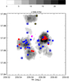 |
Fig. 1. Selected high-density regions for CARLAJ1358+5752 at z = 1.368. Passive and active galaxies are shown in red and blue, respectively. ETGs are shown as circles. LTG are shown as squares (disks) and diamonds (irregulars). The cluster spectroscopic members are marked by a small yellow circle, when they are black they are not included in our magnitude, colour and spatial selection but are shown to better explain our overdensity selection. The RLQ is shown as a star. The bar shows S/N levels. |
CARLA selected overdensities.
We go on to apply a further magnitude limit of H140 = 24.5 mag, which is the depth to which we can reliably classify galaxy morphology (see Sect. 2.6.1). We selected cluster members as those galaxies with H140 < 24.5, IRAC1 < 22.6 mag, (IRAC1- IRAC2) > –0.1, and lie within 0.5 arcmin of each overdensity peak in the cluster.
For each overdensity we calculated S/Nc as the S/N in circles of 0.5 arcmin radius when applying our complete cluster sample criterion (i.e. H140 < 24.5, IRAC1 < 22.6 mag, IRAC1 − IRAC2 > −0.1). With this more stringent criterion, we find Nbkg = 2 ± 1. S/Nc corresponds to our effective S/N in each selected overdensity. Table 3 shows the number of cluster galaxies selected in each overdensity, and the S/Nc of the overdensity. We expect that overdensities with S/Nc ∼ 10, S/Nc ∼ 15, and S/Nc ∼ 20 are contaminated with ∼20%, ∼15%, and ∼10% of contaminant galaxies, respectively.
We furthemore eliminate spectroscopically confirmed outliers from Noirot et al. (2018), the photo-spectral analysis of CARLAJ1018+0530 by Werner et al. (in prep.), and of CARLA J1753+6310 by Rettura et al. (in prep.). Our final sample comprises a total of 271 galaxies in 19 overdensities in the 16 CARLA confirmed clusters. In fact, 3 of our clusters are double structures (see Appendix B for details).
2.4. Galaxy stellar mass
Different stellar mass estimation methods and the use of different stellar population templates, priors, or rest-frame magnitudes can result in mass differences of a factor of ∼1.5 − 6 (∼0.1 − 0.8 dex) (van der Wel et al. 2006; Lee et al. 2009; Maraston et al. 2010; Raichoor et al. 2011; Pforr et al. 2012; Sorba & Sawicki 2018; Noirot et al. 2018), resulting in both underestimations or overestimations of masses at z > 1.4, depending on which methods, templates, priors, and rest-frame magnitudes are used. In our previous analysis of the CARLA sample (Noirot et al. 2016, 2018), galaxy stellar masses were derived from Spitzer/IRAC photometry.
In this work, we estimate galaxy stellar masses using an empirical method that links our mass estimates to those derived by the CANDELS collaboration (Santini et al. 2015) to be able to directly compare our results to theirs. In fact, we cannot derive masses by fitting the galaxy spectral energy distribution.
We estimated the masses of the cluster galaxies by calibrating our CARLA photometry against that of the CANDELS Santini et al. (2015) median galaxy stellar mass. This catalogue has the advantage of having been built using results from ten different teams. This enabled the authors to estimate how different parameter choices of the different teams affected their final results. Their analysis showed that the largest scatter around the median mass was produced by different choices of stellar population synthesis templates (resulting in scatter of ∼0.1 − 0.2 dex), and the inclusion of nebular emission was crucial for young galaxies (age < 100 Myr) at z > 2.2 (Santini et al. 2015). The errors on the median stellar masses include the uncertainty due to the different method assumptions and degeneracies, combined with errors on photometric and spectroscopic redshifts, which are the largest contributions to the total uncertainties. When compared to the 3D-HST published masses (Skelton et al. 2014) for the same galaxies in the GOODS-S field, they agree within ∼0.1 dex with a negative offset of ∼ − 0.1 dex for the CANDELS masses.
We used IRAC1 photometry to perform our mass calibration, but we verified that our results do not change when using IRAC2. IRAC1 corresponds to the rest-frame near-infrared in the redshift range of the CARLA clusters and it is therefore less biased by extinction than H140, which corresponds to the rest-frame U or V-band for the CARLA clusters.
We first use the CANDELS combined catalogue to obtain a linear relation between the Guo et al. CANDELS IRAC1 photometry and the Santini et al. median galaxy mass in seven bins chosen in the redshift range covered by our CARLA sample, namely, 1.35 < z < 2.8, and in the magnitude range 20 < IRAC1 < 25 mag. We accounted for errors in both parameters in our fit using the code mpfityx from Markwardt (2009). This magnitude range is well within the CANDELS IRAC1 photometric depth. The redshift bin width was chosen to have enough galaxies for stable linear fits.
We then fixed the slopes of the relations and re-fit the IRAC1-mass relation using the TPHOT-CANDELS catalogue, constraining the magnitudes to the range corresponding to the depth of the CARLA images: IRAC1 = 20–22.6 mag. The difference in the offset between the relationships we measure is typically ∼0.1 − 0.3 mag. These relations are shown in Table 4.
CANDELS mass calibration, showing the linear coefficients found for the following relations: Log10(M*) = a + b × (IRAC1) for the CANDELS combined catalogue (CC) and the TPHOT-CANDELS catalogue (TCC), and the scatter around these relations σMC.
The average difference between the median masses taken from Santini et al. and the masses derived from this calibration is −0.03 ± 0.05 dex and 0.3 ± 0.1 dex, in the redshift ranges of z = 1.35 − 2 and z ∼ 3, respectively. The scatter increases with magnitude and redshift, from ∼0.12 at redshift z = 1.35 − 1.45 to ∼0.2 at redshift z ∼ 3.
With these new mass estimates, the mass range for the spectroscopically confirmed CARLA members is 2 × 10⁸ − 3 × 10¹² M⊙, including the AGN, for which the estimated mass is an upper limit. These mass estimates are approximately four times smaller (≈0.5 dex) than those derived from stellar populations models by Noirot et al. (2018). This is consistent with the mass uncertainty estimated in Noirot et al. (2018), and it has been well documented that different stellar mass estimation methods, including the use of different stellar population templates, priors, or rest-frame magnitudes, can result in mass differences by a factor of ∼1.5 − 6 (in the range ∼0.1 − 0.8 dex) (van der Wel et al. 2006; Lee et al. 2009; Maraston et al. 2010; Raichoor et al. 2011; Pforr et al. 2012; Sorba & Sawicki 2018; Noirot et al. 2018). This difference in mass estimates does not change results from Noirot et al. (2018). The conclusions from the SFR versus stellar mass analysis (Fig. 7 in Noirot et al. 2018), for example, were also confirmed by Markov et al. (2020) for one of the clusters, and we verified that these do hold with our new mass estimates.
Since our calibration is based on the CANDELS stellar masses, our mass estimates are affected by the same systematic uncertainties as the CANDELS Santini et al. (2015) mass estimates. We estimated our total mass uncertanties by adding in quadrature the scatter around the linear relation fit σMC = 0.4 − 0.5 dex for log , and ≈0.2 dex for log
 , and the average Santini et al. (2015) systematic mass uncertainties, which are in the range of ∼0.1 − 0.2 dex. To obtain the total uncertainty on our mass measurements, we added in quadrature σMC and the average mass uncertainty from Santini et al. (2015) as a function of the redshift and the IRAC1 magnitude, and we derived mass uncertainties of ∼0.4 − 0.5 dex for log
 , and ≈0.2 − 0.3 dex for log
 . We considered that the differences due to age, dust content, and metallicity are taken into account by these mass uncertainties.
In particular, most of the mass estimate methods from Santini et al. (2015) assume a Calzetti dust extinction law (Calzetti et al. 2000). Given that quiescent ETGs at redshifts similar to ours have shown at least two orders of magnitude more dust at fixed stellar mass than for local ETGs (Gobat et al. 2018), and that the dust attenuation increases with mass in star-forming galaxies (e.g. Pannella et al. 2015), this prescription may introduce uncertainties. More sophisticated radiative transfer models predict a shallower dust attenuation curve than the Calzetti law for larger attenuation optical depths, and this impacts dust attenuation estimations in the rest-frame near-infrared at the redshifts that we are probing (e.g. Charlot & Fall 2000; Chevallard et al. 2013; Buat et al. 2018, 2019; Trayford et al. 2020), and as a consequence, the galaxy stellar mass estimation (e.g. Reddy et al. 2015, 2018). In fact, galaxy stellar masses derived assuming the Calzetti law are predicted to be ∼30% (∼0.2 dex) larger than those derived with new models (e.g. Reddy et al. 2015, 2018). This bias impacts both CANDELS mass estimates and ours and it has been included by Santini et al. (2015) in their estimation of systematic uncertainties.
In Fig. 2, we show that the galaxy stellar mass distributions for cluster overdensities in three redshift bins are consistent. The three galaxy mass distributions are similar up to z ∼ 2 and span the range  . The cluster at z = 2.8 does not show galaxies with log
 .
.
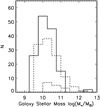 |
Fig. 2. Galaxy stellar mass distribution within the cluster overdensities in the redshift range 1.3 < z < 1.6 (continuous line), 1.6 < z < 2.1 (dashed line), and z = 2.8 (dot-dashed line). The three distributions are consistent. |
2.5. Definition of local and global environment
2.5.1. Local environment
We quantified the local environment of the cluster galaxies by deriving galaxy projected surface densities. We selected all galaxies in the whole HST field with IRAC1 < 22.6 mag and (IRAC1–IRAC2) > –0.1. We then applied the method of Nth-nearest neighbor distances:  . N is the number of galaxy neighbors, DN is defined as the distance in Mpc to the Nth nearest neighbor. Our results are stable in the range of N = 5 − 10 and hereafter we use N = 7 to be consistent with previous galaxy projected surface density estimates using HST cluster observations (e.g. Postman et al. 2005).
2.5.2. Global environment: Total stellar mass of the cluster
We quantified the global environment of each cluster galaxy in terms of the halo mass of the overdensity the galaxy resides in. We first measured the total stellar mass of each overdensity, then used the stellar mass to total mass ratio (Behroozi et al. 2013, 2019) and the correlation between the stellar mass of the brightest galaxy in the cluster and halo mass (van der Burg et al. 2014) to derive an approximate estimation of the halo masses. These halo masses should not be taken as measurements and we expect large errors (≈0.5 dex) to our rough estimation.
The total stellar mass within each overdensity was obtained by summing the galaxy stellar masses within 0.5′ of each overdensity peak. The total stellar mass of the overdensities are given in Table 3 and displayed in Fig. 3. The halo masses of the overdensities are in the approximative range  and are tabulated in Table 3.
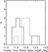 |
Fig. 3. Total stellar mass within each overdensity of the CARLA clusters in the redshift range of 1.3 < z < 1.6 (continuous line), and 1.6 < z < 3 (dashed line). These stellar masses roughly correspond to a total halo mass of |

2.6. Morphology
2.6.1. Morphology of galaxies in CARLA images
We classify the morphology of all galaxies brighter than H140 = 24.5 mag in the overdensity regions described in Sect. 2.5 in each CARLA HST image. Our classification was performed by a single person, SM, based on postage stamps of 128 × 128 pixel (16.6 × 16.6 arcsecond). From previous visual classification statistics (Postman et al. 2005; Kartaltepe et al. 2015), a morphological classification is considered stable when ∼70% of classifiers are in agreement, and we consider this as our uncertainty.
In this paper we will describe a galaxy morphologically as an ETG or a late-type galaxy (LTG). However, we wish our morphological classifications to be directly comparable to the field baseline provided by CANDELS morphologies classified by Kartaltepe et al. (2015). We therefore have followed the more complex visual morphology classification scheme of Kartaltepe et al. (2015), and later convert these classifications into ETG and LTG classes. We classify each galaxy as a: (1) Disk: galaxies that have a disk even if they don’t show clear spiral arms; (2) Spheroid: galaxies that are resolved spheroids and do not show a disk; (3) Irregular: all galaxies that cannot be classified either as a disk or spheroid; (4) Compact or unresolved: compact or unresolved galaxies; (5) Unclassifiable.
The only difference between this scheme and that of Kartaltepe et al. (2015) is that our Disk class include galaxies classified as either disk or disk spheroid by Kartaltepe et al. (2015; see Sect. 2.6.2 for more details). We furthermore assign a ‘morphology quality flag’ to each galaxy classification: 1. certain; 2. uncertain.
In addition to the above morphological classes, we also followed Kartaltepe et al. (2015) in identifying mergers. These are defined as galaxies that show visual tidal features or other structures that may indicate a recent merger has occurred. This class corresponds to galaxies that have Kartaltepe et al. fM > 2/3, which are ∼1.1 ± 0.1% of the galaxies in our ‘combined CANDELS catalogue’.
We also add structure flags similar to Kartaltepe et al. (2015): 1. tidal arms; 2. double nuclei; 3. asymmetric; 4. spiral arms/ring; 5. bar; 6. point source contamination ; 7. edge-on disk; 8. face-on disk; 9. tadpole galaxy; 10. chain galaxy; 11. disk- dominated; 12. bulge-dominated. Most of these flags do not occur enough in our galaxy magnitude or colour and mass ranges to be statistically significant for this work, except the asymmetric flag. Therefore, we do not consider them in the statistics presented below, but these classifications are available from the lead author upon request.
For this paper, given the small numbers of galaxies in each category for both CANDELS and our sample, we combined spheroids and compact, unresolved, point sources in an ETG single class, and disks, disk spheroids, and irregulars in a LTG single class. The sample used in this paper does not include any unclassifiable galaxy.
2.6.2. Morphology of galaxies within CANDELS
Kartaltepe et al. (2015) visually classified the morphologies of galaxies in the CANDELS GOODS-S field to a depth of H160 = 24.5 mag. This matches well our magnitude limit of H140 = 24.5 mag in the CARLA images. Both H140 and H160 are in the optical rest-frame range for galaxies at redshift 1.5 < z < 2.8 and, as Kartaltepe et al. (2015) pointed out, morphology classifications performed in infrared bandpasses at these redshifts do not show significant differences.
Each CANDELS galaxy was classified by at least three people into the same morphological classes listed above; Spheroid, Disk, Irregular, Unresolved/Point Source, Unclassifiable. They also considered mixed classes, and labelled other features such as face-on disk or tadpole galaxy. Full details of these additional classifications can be found in Kartaltepe et al. (2015).
The catalogue from Kartaltepe et al. also provides the fraction of classifiers that identify each galaxy as belonging to a given class. Here, fsph/disk/irr/tp refers to the fraction of classifiers that identify each galaxy as a spheroid, disk, irregular, or tadpole galaxy; fps refers to the fraction of classifiers that identify the object as a point source; and func refers to the fraction of classifiers that could not classify the object. We use these fractions as proxies of the probability that a galaxy belongs to a given morphological class.
In the Kartaltepe et al. (2015) classification, each galaxy can be classified into more than one class with high probability. For this reason, we are using the following criteria to place galaxies into each of the five dominant classes:
-
Spheroid: fsph > 2/3 and fdisk < 2/3, or 0.5 < fsph < 2/3 and fdisk < 0.5 and firr < 2/3. Spheroids are ∼20% of the galaxies in our ‘combined CANDELS catalogue’.
-
Disk: fdisk > 2/3 and fsph < 2/3, or 0.5 < fdisk < 2/3 and fsph < 0.5 and firr < 2/3. Galaxies with this morphology comprise ∼60% of our ‘combined CANDELS catalogue’. We add to this class galaxies with fdisk > 2/3 and fsph > 2/3. These disk galaxies have a prominent bulge and comprise ∼6% of the galaxies in our ‘combined CANDELS catalogue’. Hence, ∼66% of the galaxies in our ‘combined CANDELS catalogue’ are disks.
-
Irregular: firr > 0.5 and fdisk < 2/3 and fsph < 2/3. Or ftp > 2/3. Irregulars comprise ∼13% of the galaxies in our ‘combined CANDELS catalogue’.
-
Compact, unresolved, or point source: fps > 2/3. These sources comprise ∼1% of the galaxies in our ‘combined CANDELS catalogue’.
-
Unclassifiable: func > 2/3, or galaxies that do not belong to the classes above. This comprises ∼1% of the galaxies in our ‘combined CANDELS catalogue’.
The limit of 2/3 (∼70%) corresponds to the typical agreement on galaxy visual morphology from multiple classifiers (e.g. Postman et al. 2005). The sum of the fractions in each class do not add up to 100 because they are rounded numbers.
2.7. Passive and active galaxy selection
Nine of our CARLA clusters have been observed in the i or z-band from the ground (Table 2). For these clusters, we use colour-colour diagrams, based on the UVJ diagrams commonly used in the literature, to separate passive from active galaxies (e.g. Labbé et al. 2005; Wuyts et al. 2007; Williams et al. 2009; Whitaker et al. 2011; Fang et al. 2018) in clusters with ground-based observations. Unfortunately, our limited spectral energy coverage (of only four bands per cluster) means we are unable to perform spectral energy distribution fitting and derive rest-frame UVJ colours. Instead we use the colours of the observed bands since, at the redshift range of our clusters, the i-band and z-band observations correspond approximately to the rest-frame U-band, whilst H140 and IRAC1 correspond to approximately the rest-frame V and J-band, respectively. When the U-band rest-frame is not available, the FUV rest-frame can substitute it and even lead to more precise specific star formation rate (sSFR) measurements (Arnouts et al. 2013; Leja et al. 2019).
We used apparent magnitude colours to define passive regions of i − H140 IRAC1 and z − H140 IRAC1 colour space as shown in Fig. 4, which shows the 271 galaxies selected for this paper analysis. We define as quiescent galaxies with log(sSFR) < −9.5 [yr−1], which characterises the quiescent region at our cluster redshifts (e.g. Whitaker et al. 2014; Leja et al. 2019). The method used to obtain these colours is based on a calibration on CANDELS apparent magnitudes, and is described in Appendix C.
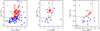 |
Fig. 4. Cluster colour-colour diagrams. Left: All clusters observed with ACAM. Middle: all clusters observed with GMOS. Right: CARLAJ2039-2514, observed with ISAAC. The continuous lines limit the regions that separate passive from active galaxies. Passive and active galaxies are shown in red and blue, respectively. ETGs are shown as circles. Disks and Irregular galaxies are shown as squares and diamonds, respectively. The cluster spectroscopic members show a yellow dot at the center. The RLQ and HzRG are shown as yellow stars and triangles, respectively, and have spectroscopic redshift even if we do not mark them with a dot. The other AGN have colours that are not included in the plots. The crosses on the upper left are the average colour errors. |
Among the 271 galaxies selected for the study in this paper, only 10 are spectroscopically confirmed members and have sSFR measurements (Table 5). Of those, 6 (∼20% of the total selected passive population) are classified as passive galaxies and have log(sSFR) < −9.5 [yr−1] at ∼1σ. The other 4 are classified as active, and 3 of them have log(sSFR) < −9.5 [yr−1] at ∼2σ. This confirms that our selection includes recently quenched star-forming galaxies (see appendix), and that many of star-forming galaxies in the CARLA clusters show SFR that are ∼3σ below the field main sequence (Noirot et al. 2018).
CARLA-selected spectroscopically confirmed member classification as passive and active galaxies in this paper.
All the AGN have log(sSFR) > −9.5 [yr−1] and are found in the active galaxy region, except the CARLAJ1753+6310 AGN that is found in the passive galaxy selection and has a log(sSFR) = −8.6 ± 0.3 [yr−1]. The AGN that are not included in the plots have colours that are not in the figure range. The fraction of the galaxies that could not be classified as passive and active corresponds to ∼30% of the galaxies.
3. Results
We calculated the galaxy type fractions as the ratio of galaxies in each category divided by the sum of total galaxies. The exception is the ETG fraction which we calculate with respect to the total of ETGs plus the LTG population (excluding the QSO). We used statistical background subtraction to correct for foreground and background galaxies that contaminate our cluster sample.
Following the method detailed in Postman et al. (2005), we calculated the corrected number of galaxies in our clusters as Ncorr = Nuncorr + Nmiss − Ncont, where Nuncorr is the number of galaxies of each sub-type, without correcting for contamination; Nmiss are the galaxies that we missed by applying our selection criteria; Ncont are the foreground and background galaxies that are not at our cluster redshift and are estimated to contaminate our sample – for each fraction category.
We estimated Nmiss and Ncont for each galaxy sample using the CANDELS combined catalogue. Within our colour, magnitude and mass selection, and in a circle of radius 0.5 arcminutes, we typically detect 2 ± 1 galaxies in the CANDELS combined catalogue. Of these galaxies, 28 ± 2% are ETGs, 21 ± 1% are passive, 34 ± 2% are asymmetric, and 1.7 ± 0.5% are mergers. We used these numbers to correct the cluster galaxy counts for fore- and background contaminants, namely, Ncont, within each subsample of galaxies; Ncont is typically is in the range 3 − 15%. The fraction of missing galaxies is negligible (< 2% for each category), and we approximated Nmiss ∼ 0.
The percentage of CARLA active ETGs with respect to the total number of ETGs is 20 ± 6% at 1.35 < z < 1.65, and 55 ± 13% at 1.65 < z < 2.05, compared to 6 ± 5% in the ‘TPHOT-CANDELS catalogue’ and 6 ± 5% in our ‘CANDELS combined catalogue’ for galaxies selected in the range 1.3 < z < 3. In general, this shows a large percentage of active ETGs in CARLA clusters with respect to the field, especially in the highest redshift range of our sample.
We list the corrected fraction of passive, ETG, asymmetric, and interacting galaxies in each cluster in Table 6. Many clusters show enhanced fractions in all categories, but the uncertainties on these fractions are large because the number of galaxies in each cluster is small. We therefore combine all the cluster galaxies into a single sample to explore the effect of stellar mass and environment on the morphology and passivity of the cluster galaxies. In the appendix (Fig. D.1), we show the ETG and passive fractions as a function of cluster redshift. We find no correlation between these fractions and redshift, with Pearson coefficients of p = −0.03 and p = −0.003 for ETGs and passive galaxies, respectively. This also justifies our decision to combine all the cluster galaxies into a larger sample.
Corrected fractions of passive galaxies, ETGs, and mergers, and the minimum, maximum, and median ΣN and galaxy stellar mass  .
.
3.1. Influence of local environment on the morphology and passivity of cluster galaxies
We first explore the fraction of passive galaxies within the clusters as a function of the local environment, shown in Fig. 5. We also split the cluster sample into a higher and lower redshift bin to explore whether there is any redshift evolution. We find there is a strong relation between the fraction of passive galaxies and the local environment of a cluster galaxy. Furthermore, we find no significant difference in this relationship between clusters at 1.3 < z < 1.6 and 1.6 < z < 2. This result extends the work of Lemaux et al. (2019) and Tomczak et al. (2019) that found the SFR-density relation is already in place at z ∼ 1.5.
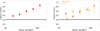 |
Fig. 5. Passive galaxy fractions as a function of environment. Left: Our entire sample. Right: passive fractions in two redshift bins: 1.3 < z < 1.6 (orange circles) and 1.6 < z < 2 (yellow circles). The grey region shows the ±1 σ range of the CANDELS passive fraction. We observe a significant passive-density relation up to z ∼ 2. |
We then explore the influence of local environment on the morphological properties of cluster galaxies. We start by examining the fraction of ETGs, also subdividing the analysis by redshift bins. We find that the ETG fractions are correlated with local environment (Pearson coefficient p ∼ 0.93). The ETG fraction decreases in the last bin, however, this drop is dominated by that lack of ETG and a high incidence of disk and irregular galaxy interactions in the high density regions of only one cluster, CARLAJ0800+402. When this cluster is excluded from the analysis, the drop is mitigated and the Pearson coefficient for the correlation between the ETG fraction and local environment is p ∼ 0.98. These correlations, shown in Figs. 6–8, demonstrate that the morphology-density relation is present in high redshift clusters.
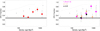 |
Fig. 6. ETG galaxy fractions as a function of environment. Left: Our entire sample. Right: ETG fractions in two redshift bins: 1.3 < z < 1.6 (magenta circles) and 1.6 < z < 2.8 (pink circles). We also show with two black circles the fraction for CARLAJ1017+6116 at z = 2.8. The small grey circles and error bars and the dashed line show the morphology-density relation at z ∼ 1 from Postman et al. (2005) and at lower redshift from Dressler (1980). The grey region shows the ±1 σ range of the CANDELS ETG fraction. We observe a significant morphology-density relation up to z ∼ 2. The cluster at z = 2.8 shows a similar fraction of ETGs as in the other clusters, however, one cluster does not provide enough statistics to confirm that the morphology-density relation is already in place at z ∼ 3. In fact, ETG fractions are correlated with environment and increase from high to lower redshift in the intermediate dense regions. |
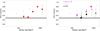 |
Fig. 7. ETG galaxy fractions as a function of environment. Details are the same as in Fig. 6, excluding the cluster CARLAJ0800+4029, which shows an high percentage of mergers in its densest regions. We observe a significant morphology-density relation up to z ∼ 2. The ETG fractions drop in the last bin, which is observed in the entire sample (see Fig. 6), is mitigated. This means that the mergers in the high density regions in CARLAJ0800+4029 were dominating the ETG fraction drop observed when including this cluster in the analysis. |
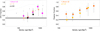 |
Fig. 8. ETG (left) and passive (right) galaxy fractions as a function of environment. Details are the same as in the right panels of Fig. 5 and Fig. 7, excluding the cluster CARLAJ0800+4029, and separating the z ∼ 2 clusters from the others at z < 1.9. This shows that the relations holds at z ∼ 2. |
The morphology-density relation is most clearly present in the lowest redshift bin, and holds up to z = 2. The cluster at z = 2.8 only has galaxies in two local density bins and the data are consistent with both the field values and with the morphology-density relation within uncertainties. We therefore conclude that the morphology-density relation is present in clusters up to z = 2, but there is no strong evidence for or against this relationship persisting at higher redshifts.
We compare our high-redshift cluster sample to data from the local Universe (Dressler 1980) and at z ∼ 1 (Postman et al. 2005). These are displayed in Figs. 6 and 7 as the dashed line and the small grey circles. We find that the ETG fractions in high-redshift clusters are consistent with those observed in clusters at z ∼ 1 by Postman et al. (2005) when the local density is ΣN > 700 gal/Mpc2. Thus, there is already a strong morphological influence occurring in the densest local environment of clusters at z = 2. However, at this high-local density, the ETG fraction of z = 1 clusters and our 1.3 < z < 2 CARLA clusters is lower than that of clusters in the local Universe. This suggests that further morphological transformation must still occur within the cluster population.
At lower local densities, where ΣN < 700 gal/Mpc2, the CARLA clusters exhibit a similar ETG fraction as the field. This is in stark contradiction to clusters at z = 1 that already exhibit higher ETG fractions. It therefore seems that the densest of cluster environments influence the morphology of galaxies first, with lower density local environments either taking longer to influence galaxy morphology or only influencing galaxy morphology at later cosmological times.
3.2. Influence of global environment on the morphology and passivity of cluster galaxies
In Fig. 9, we show the ETG and passive galaxy fractions as a function of global environment defined as total galaxy stellar mass in the overdensity. The morphology and passivity of cluster galaxies do not depend on the cluster total stellar mass (the Pearson coefficient is p = −0.2 and p = −0.4 for the ETG and passive fractions, respectively). As shown in the Appendix D, this lack of correlation is also observed with the overdensity S/N, as a proxy of density contrast.
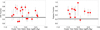 |
Fig. 9. ETG and passive galaxy fractions as a function of global environment defined as total galaxy stellar mass in the overdensity. The grey region shows the ±1σ range of the CANDELS fractions. |
3.3. Influence of stellar mass on the morphology and passivity of cluster galaxies
We examine how stellar mass influences the ETG and passive fractions in Fig. 10. The ETG and passive galaxy fractions are displayed in two mass bins and also subdivided into two redshift bins: 1.3 < z < 1.6 and z > 1.6. At both redshifts, more massive galaxies show higher ETG and passive fractions, but the uncertainties are high, so we do not record a conclusive relationship in either case. This holds even when considering more mass bins, however, the uncertainties rise because we are selecting fewer galaxies in each bin and the field contamination correction is also more uncertain.
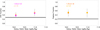 |
Fig. 10. ETG and passive galaxy fractions as a function of mass in two redshift bins: 1.3 < z < 1.6 and z > 1.6. Symbol colours are the same as in Fig. 5. The grey region shows the ±1σ range of the CANDELS fractions. The ETG and passive fractions mildly increase with increasing mass. |
Figures 5 and 6 display a strong relationship between the local environment and the ETG and passive fractions. To explore whether these relations are caused by an underlying correlation between galaxy stellar mass and local environment, we plot in Fig. 11 the ETG and passive fractions as a function of environment in two mass bins:  and
and  . While the two separate samples are less statistically significant, the morphology and passive density relations are in place in both mass bins. For the ETG fractions, less massive galaxies have lower ETG fractions (on average) than the more massive galaxies, while in the densest and least dense bins they are consistent with the field. However, as in Fig. 10, the uncertainties are too large to make strong conclusions. We investigate whether there is a relationship between galaxy stellar mass and local environment, but we find that these parameters are not correlated in our cluster sample, with a Pearson coefficient of p = 0.11. This implies that the morphology-density and passive galaxy density relations are not driven by a correlation between galaxy mass and environment.
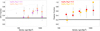 |
Fig. 11. ETG and passive galaxy fractions as a function of galaxy surface density in two mass bins: |


In conclusion, we find that the morphology-local density and passive-local density relations are already in place by z = 2 for all galaxies with stellar masses above our mass limit,  , but we cannot determine their dependence on stellar mass.
3.4. Merger fractions of z > 1.3 cluster galaxies
We concentrate on visually classified mergers rather than the number of close companions because the fractions of close companions can be biased by projection effects in clusters. The merger fraction for the entire sample of cluster galaxies is 26 ± 3%, which is significantly higher than the CANDELS average merger fraction of 1.7 ± 0.5. In Fig. 12, we display the merger fraction as a function of local environment and mass. The merger fraction is systematically higher (≳3σ, except at high density where uncertainties are high) than the CANDELS merger fraction. Merger fractions show a moderate correlation with mass at all redshifts, with higher fractions for more massive galaxies and lower redshifts. However, similarly to the results given in Sect. 3.3, this result is not statistically significant because the differences in the observed fractions is consistent within ∼1σ. In contrast to the passive and ETG fractions, the merger fraction shows no significant correlation with local environment. We explore the implications of this in the discussion below.
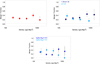 |
Fig. 12. Merger fractions as a function of environment. Top left: Our entire sample. Top right: Merger fractions in two redshift bins: 1.3 < z < 1.6 (dark blue circles) and 1.6 < z < 2.8 (light blue circles). Bottom: Merger fractions as a function of galaxy stellar mass. The grey region shows the ±1 σ range of the CANDELS merger fraction. The merger fraction in our cluster sample is significantly higher than in CANDELS and shows a moderate correlation with environment and mass. |
We additionally observe an average asymmetric galaxy fraction of 50 ± 3%, which is significantly larger than the CANDELS asymmetric fraction of 34 ± 2%. This provides supporting evidence that merger rates are enhanced in the cluster environment. Our asymmetric galaxy fraction has no dependency on stellar mass, local or global environment, or redshift.
3.5. AGN and spectroscopically confirmed member morphology
The CARLA central AGN are eight high redshift radio galaxies (HzRG) and eight quasars (RLQ). We also confirmed two more quasars, one in the CARLAJ1510+5958 area, but at a different redshift (z = 1.838) and one spectroscopically confirmed member in CARLAJ0800+4029 (Noirot et al. 2018). The RLQ all have unresolved morphology, often saturated and/or showing diffraction spikes. The HzRG morphologies are shown in Fig. 13: they are spheroids, disks, and irregulars. They are often found with a companion and tidal tails, and some are asymmetric, evidence for possible interactions or mergers. The radio source in CARLAJ2355–0002 has been discussed in Noirot et al. (2018). Collet et al. (2015) reported a peculiar radio-jet and gas properties in this radio source, which they found similar to the properties of the brightest cluster galaxies in low-redshift cool core clusters. Noirot et al. (2018) already discussed the morphology of this object in detail, and our HST image shows two sources and a complex morphology for this object. We do not use this galaxy pair in the galaxy morphology and colour analysis in this paper. Its colours are consistent with being an active galaxy, and its morphology does not have a clear classification.
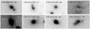 |
Fig. 13. Morphology of the eight central HzRG. They all show possible interactions and tidal arms. The radio source in CARLAJ2355–0002 has been discussed in Noirot et al. (2018). |
The CARLA spectroscopically confirmed members with a morphological classification (107 galaxies), are mostly disks (55%), even if a large percentage of confirmed members are star-forming spheroids (∼22%; 4 of 23 are HzRG) and visually compact galaxies (∼20%). Only ∼4% are irregular galaxies. Figure 14 shows the member morphology distribution. Excluding the AGN, the members that have sSFR 3σ higher than the field main sequence (with log(sSFR) ≳ −8.2 [yr−1] at z < 1.5, and log(sSFR) ≳ −7.8 [yr−1] at 1.5 < z< 2; from Whitaker et al. 2014) are nine disks and one spheroid at z < 1.5. Three disks show interaction (two also show tidal tails), and eight are asymmetric, indicating a possible connection between recent merger and starburst activity. At 1.5 < z< 2, we find one visually compact galaxy in CARLAJ1129+0951 with log(sSFR) ≳ −7.8 [yr−1] that does not show interactions, tidal tails, or asymmetry.
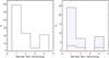 |
Fig. 14. Morphology of the spectroscopically confirmed cluster memberss. Left: Morphology class distribution of the 107 spectroscopically confirmed cluster members from Noirot et al. (2018), shown on the left. The classes are: Disk (1), Spheroid (2), Irregular (3), Compact (4), Unclassifiable (5). Most of the members are disks, however there are large percentages of star-forming spheroids and compact galaxies. Right: Morphology class distribution of the members that have ground-based photometry is shown on the right. The blue and red lined histograms correspond to active and passive galaxies, respectively. The passive LTG are galaxies with star formation rates below the field main sequence. |
4. Discussion
4.1. Structure and heterogeneity of protoclusters
Cosmological models predict that the clusters observed in the local Universe are built via the accretion of groups and filaments. At the redshifts of our sample, the main cluster progenitors are predicted to have halo mass in the range of  and are expected to be surrounded by groups of similar or lower mass, spread out over scales of ≈35 h−1 Mpc2 comoving at z ∼ 2, which will accrete to form the clusters observed in the local Universe (Chiang et al. 2013; Muldrew et al. 2018).
Our CARLA clusters have estimated halo masses of  and so are consistent with these model predictions. Nine of our clusters have expected total halo masses of log
 , which defines a galaxy cluster2. All others have an expected halo mass consistent with massive groups, which potentially are the main progenitors of local clusters.
Our images do not cover large enough scales to observe the entire infall regions, but we do observe some structure. We observe three double structures (CARLAJ1018+0530, CARLAJ1358+5752, CARLAJ2039–2514) and multiple less significant overdensities in all our clusters except CARLAJ1753+6310. In all double structures, one of the two overdensities reaches ΣN ≳ 600 gal Mpc−2, and median ΣN > 300 gal Mpc−2, typical of cluster core environments at z ∼ 1 (e.g. Postman et al. 2005; Lemaux et al. 2019), and the other one has densities of ΣN ≲ 600 gal Mpc−2, typical of groups infalling in clusters (e.g. Mei et al. 2012; Lemaux et al. 2019).
This results is consistent with the CARLA overdensities being clusters, groups and proto-clusters in the epoch of assembling. The exact characteristics of the assembly regions can only be better analyzed using a large imaging and spectroscopy coverage of these field.
Our local density analysis reveals that the galaxy populations within the cores of these high redshift clusters and protoclusters are heterogeneous: some consistent with the field, others with lower redshift groups and clusters. Around 25% of our structures clearly show environments and galaxy fractions consistent with groups and filaments. For example, CARLAJ0958–2904 does not show properties much different from the field; whereas around 30% of our clusters have very dense local environments with ΣN > 1000 gal Mpc−2, and here the galaxy population exhibits ETG or passive fractions of > 50%. Two clusters, CARLAJ1052+0806 and CARLAJ1753+6310 (both at z ∼ 1.6), exhibit ETG and passive fractions that are consistent with being mature clusters as those at z < 1.3.
The other structures are a more heterogeneous sample, mostly showing ETG and passive fractions and expected halo mass characteristic of groups and clusters, consistent with what is expected for cluster and proto-clusters at these redshifts. One exception to the general trends is a structure with low-density environment 110 ≲ ΣN ≲ 220 gal Mpc−2, CARLAJ1103+3449, with expected halo mass that corresponds to a group, in which galaxy pre-processing has already happened. The central AGN is a star-forming ETG and its central region hosts a massive molecular gas reservoir (Markov et al. 2020), which suggests massive cool gas flows similar at those observed in the local Universe.
These results are consistent with a large body of literature on individual clusters. Clusters and proto-clusters at z > 1.5 show a large variety in their galaxy populations. Some samples show large quiescent population and already quenched star-forming galaxies (Andreon & Huertas-Company 2011; Cooke et al. 2015; Strazzullo et al. 2015, 2016; Noirot et al. 2018; Markov et al. 2020; Shi et al. 2021; Sazonova et al. 2020), others show enhanced star-formation in their cores (Tran et al. 2010; Fassbender et al. 2011; Hayashi et al. 2011, 2016; Tadaki et al. 2012; Zeimann et al. 2012; Brodwin et al. 2013; Mei et al. 2015; Alberts et al. 2016; Shimakawa et al. 2018; Aoyama et al. 2022; Koyama & del Polletta 2021; Polletta et al. 2021; Zheng et al. 2021), and then others show both populations (Wang et al. 2016; Kubo et al. 2017; Strazzullo et al. 2018).
At higher redshift (z > 2), some dense structures (clusters and protoclusters) present starbursts (Casey et al. 2015; Casey 2016; Wang et al. 2016), but others high fractions of quiescent galaxies (McConachie et al. 2022). Our findings stand in contrast to the enhanced star-formation and starburst activity in these samples, since we find an increasing fraction of passive galaxies in the densest local environments. This difference with other samples is probably due to the different sample selection, where some overdensities have been detected using star-forming and starburst galaxy colour selection, while others have been found by red galaxies overdensities and X-ray emission.
From our results, the CARLA overdensities selected around RLAGN have a more passive and ETG-dominated galaxy population than the overdensities selected using star-forming and starburst galaxy colour selection, while they show similar populations as those found in X-ray and SZ selected clusters at z ≲ 1.5 (e.g. Postman et al. 2005; Mei et al. 2009; Andreon & Huertas-Company 2011; Strazzullo et al. 2016, 2019; Lemaux et al. 2019; van der Burg et al. 2020). This might indicate a different evolution stage in the overdensities selected by different methods, with those selected using star-forming and starburst galaxy colour selection being still in a stage in which morphological transformations and quenching are still happening, in contrast with the galaxy population in CARLA, X-ray, and SZ selected clusters that show large fractions of ETGs and passive galaxies up to z = 2 − 3.
Our sample shows different percentages of ETGs and passive galaxies in cluster regions that are otherwise similar in terms of global environment, dynamical state, and redshift. We would therefore warn that ETGs and passive fractions in individual high-redshift clusters or protoclusters should not be used to conclude whether or not morphological transformations or quenching happened first. This suggests that physical processes that lead to morphological transformations and quenching are often correlated but might not be exactly the same and can happen independently one from the other. Some models (De Lucia et al. 2012; Laigle et al. 2018) predict that these differences might be due to the fact that galaxies have different pre-processing histories that depend on the environments they were hosted by before their accretion in clusters and on tides in filaments that impact galaxy mass and quenching. In fact, some of the galaxies observed in our denser regions might have been accreted in much earlier epochs and others more recently, with different levels of pre-processing in the groups and filaments that hosted them in their previous history.
The unique prospective from the CARLA survey is that by combining our large sample of clusters and protoclusters at z > 1.3, we are able to average over a range of accretion histories and examine trends with both stellar mass and environment.
4.2. Morphology and SFR-density relations of CARLA clusters in the context of prior results
Our main result is that galaxy morphology and passivity are strongly correlated to local environment by z ∼ 2. We find the ETG and passive galaxy fractions are higher in denser environments. These fractions also mildly depend on galaxy stellar mass, with ETGs and passive galaxies also being the most massive. However, we find no correlation with the global environment (assuming that the central total stellar mass is correlated with total halo mass using Behroozi et al. 2019).
These results are reminiscent of the well-defined morphology-density relation that is in place at z ≲ 1 (e.g. Dressler 1980; Postman et al. 2005). The densest regions in the Universe are found in galaxy clusters, which host high percentages (≳80%) of passive ETGs. Dense cluster environments can change galaxy morphologies and quench star formation via interactions between the galaxy and the intracluster medium or gravitational potential, or by galaxy-galaxy interactions which are frequent in the dense clusters. Quenching and morphological transformations are also observed to be correlated with galaxy mass, with more massive galaxies being more passive and more likely to possess ETG morphologies (Peng et al. 2010). In this case, quenching and morphology transformations are consequences of mass accretion and the formation of a bulge.
These studies have been extended to higher redshifts using field surveys. These works find that passive fractions are higher for massive galaxies up to z ∼ 2 − 3 (Ilbert et al. 2013; Muzzin et al. 2013; Tomczak et al. 2014). Darvish et al. (2015, 2016, 2018) have studied galaxy properties as a function of environment in the COSMOS field up to z ∼ 3 (see also Lemaux et al. 2022). They found that the passive galaxy fraction depends on the environment at z ≲ 1 and on stellar mass out to z ∼ 3. They suggested that at z ∼ 1 the denser environment could quench massive galaxies in a more efficient way because of the higher merger rate of massive galaxies in denser environments. In their field sample, less massive galaxies ( ) are quenching, while more massive galaxies exhibit starbursts.
With the CARLA cluster galaxies, we find that both the ETG and passive fractions depend on environment and only mildly on galaxy stellar mass. The explanation for this discrepancy is that we probe a very different environment as compared to earlier field studies. COSMOS covers an area of only few degrees and does not host a significant cluster population. Most COSMOS galaxies are hosted in environments with a projected galaxy surface density of Σ ≲ 300.
At Σ ≲ 300, the CARLA clusters also exhibit ETG and passive fractions that are similar to the field. Thus, our results are in complete agreement with the results of Darvish et al. (2015, 2016, 2018). We only observe a significant enhancement in the ETG and passive fractions at Σ > 700. Therefore, we should be wary of studies that look for environmental trends without exploring cluster environments.
One study that explored dense environments at high redshift is the Observations of Redshift Evolution in Large-Scale Environments (ORELSE; Lubin et al. 2009; Tomczak et al. 2017). This collaboration studied a large range of environments, including groups around clusters at a scale of ∼10 − 15h−1 proper Mpc in the redshift range 0.55 < z < 1.4. Using this sample, Lemaux et al. (2019) found that the average passive fraction is ∼10%, ∼ 40%, and ∼60% in three environments: lower galaxy surface density log(1 + δ) < 0.3, intermediate 0.3 < log(1 + δ) < 0.7, and higher log(1 + δ) > 0.7, respectively. Their definition of local density is  , where ΣVMC is calculated with a Voronoi Monte-Carlo (VMC) method and
  is the background local density.
The three surface density bins considered in ORELSE roughly correspond to our ΣN < 140 gal Mpc−2 (log(1 + δ) < 0.3), 140 < ΣN < 350 gal Mpc−2 (0.3 < log(1 + δ) < 0.7), and ΣN > 350 gal Mpc−2 (log(1 + δ) > 0.7). To derive this correspondence, we have calculated our background surface density  from the ‘combined CANDELS catalogue’ and we have relied on results from Darvish et al. (2015), showing that the density fields measured with ΣVMC and ΣN are in good agreement. Using this conversion, we see that our results for the passive fraction of z > 1.3 cluster galaxies agrees with ORELSE results at z < 1.4. The CARLA sample extends the relation between local density and SFR & morphology up to z = 2.
It is interesting that we find average passive fractions that are consistent with those found in Lemaux et al. (2019), showing a lack of significant passive fraction redshift evolution at fixed environment from the ORELSE survey (0.55 < z < 1.4) to our passive galaxy sample (1.3 < z < 2).
Van der Burg et al. (2020) studied passive galaxy fractions in eleven clusters from the Galaxies in Rich Early Environments (GOGREEN; Balogh et al. 2017) survey at 1 < z < 1.4. They find that the passive fraction strongly depends on galaxy mass, ranging from ∼0.3 to ∼1 at masses of  and
and  , respectively. A similar result is observed in the ZFOURGE survey (Kawinwanichakij et al. 2017) and in galaxy groups at 0.1 ≲ z ≲ 2.3 detected in deep near-infrared surveys by Sarron & Conselice (2021). Furthermore, in a sample of five clusters at 1.4 < z < 1.7 identified in the South Pole Telescope Sunyaev Zel’dovich effect (SPT-SZ) survey, Strazzullo et al. (2019) found that the passive galaxy fraction depends on both mass and environment with efficient suppression of star formation occurring at z ≳ 1.5.
In contrast to these works, the CARLA sample does not exhibit a strong stellar mass dependency for either the ETG fraction or the passive galaxy fraction. We stress that the uncertainties on our results on the mass-dependency are large and our lack of evidence of a dependency is not in disagreement with previous works within uncertainties. Our method, using statistical background subtraction, and estimating stellar masses using only IRAC1 photometry means that our mass estimates are more uncertain than the works mentioned above.
4.3. Cause of morphological transformations in high-redshift clusters
Morphological transformations of galaxies can occur through multiple routes. Rapid mass accretion resulting in a starburst can go on to form a bulge and transform LTGs into ETGs. Another route to forming an ETG morphology is through mergers and galaxy-galaxy interactions. In fact, ETG quenching can happen in different ways and at different epochs. While spheroids are formed as a consequence of starbursts and dissipative collapse, they can also form from gas-rich disk mergers that do not cause starbursts (e.g. Mo et al. 2010). If these galaxies do not accrete further gas, the spheroids resulting from the merger will become ETGs. If these merger remnants accrete substantial amounts of gas, then a disk will reform and the galaxy will present an LTG morphology.
In our sample, the passive galaxy fraction increases in denser local environments and we do not observe large fractions of star forming galaxies in dense environments. We also do not observe enhanced starburst activity in the cluster cores. In fact, excluding the AGN, we only find nine disk galaxies and one spheroid at z < 1.5 that have sSFR 3σ higher than the main sequence (log(sSFR) ≳ −8.1 [yr−1] at z < 1.5, and log(sSFR) ≳ −7.8 [yr−1] at 1.5 < z < 2), and only one visually compact galaxy at z > 1.5 in CARLAJ1129+0951, which does not show interactions, tidal tails, or asymmetry. On the other hand, three disks do show interaction (two also show tidal tails), and eight are asymmetric, indicating a possible connection between recent merger and starburst activity.
The lack of enhanced star-formation and starburst activity in the CARLA sample suggests that morphological transformations are not caused primarily by rapid mass accretion that results in a starburst and formation of a bulge. Alternatively, these starbursts may have already occurred and caused the morphological transformations, or they are heavily dust-obscured and therefore not detectable in our optical and near-infrared analysis. However, an analysis of the AllWISE3 catalogue sources in the area covered by our Spitzer observations shows that only our radio sources are detected in the 22 μm channel, which is the Wide-field Infrared Survey Explorer (WISE, Wright et al. 2010) W4 channel. This also indicated the absence of sources with high star-formation rates. In fact, this channel is closer to the peak of the infrared emission by star-forming galaxies and the lack of significant detections means that there are no intense star-forming galaxies in the area (e.g. Hwang et al. 2012; Chang et al. 2015; Cluver et al. 2017).
On the other hand, previous studies concluded that a high fraction of mergers in clusters at z > 1.5 would have been necessary to explain their high quiescent fractions at z ∼ 1 − 1.5 (Darvish et al. 2015, 2016, 2018; Lemaux et al. 2019). We indeed observe merger fractions that are systematically higher than in the CANDELS fields in the CARLA clusters. Our average merger fraction is 26 ± 3%, which is significantly higher (≳3σ) than the CANDELS average merger fraction of 1.7 ± 0.5.
At first look this seems to point towards galaxy interactions and mergers acting as the primary cause of transforming LTGs into ETGs. However, whilst the ETG and passive galaxy fractions strongly increase with local environment, the merger galaxy fraction is approximately constant across all local environments. In fact, the galaxy merger fraction in the CARLA clusters is not correlated with local or global environment, redshift, or galaxy stellar mass. Therefore, the merger rate is enhanced to the same level in the low-density cluster environments (where the passive and ETG fractions are low) as in the high-density cluster environments (where the passive and ETG fractions are high). So mergers do not seem to be solely responsible for the morphological transformations and quenching.
One possibility solution that is consistent with the data from the CARLA galaxy morphologies is the theory of that the LTG or ETG morphology results from the amount of gas accreted after a merger (e.g. Zavala et al. 2019; Harshan et al. 2021). Let us take the merge fraction data at face value and presume that mergers occur at the same rate in all regions of the high redshift clusters. In the low-density regions, new disks may be able to re-form around these merger remnants through the inflow of substantial amounts of pristine gas through cold streams. However, if cold streams are disrupted in the densest regions of the clusters (as suggested by Dekel et al. 2009), then the merger remnants in the densest regions will become ETGs. Such a scenario would account for our observations of a strong morphology-local density and SFR-local density relation within clusters, as well as with a high merger rate in all cluster environments.
4.4. Active ETGs
We find higher percentages of active ETGs in CARLA clusters compared to the field, mainly within the highest redshift range of our sample. In fact, CARLA active ETGs are 21 ± 6% and 59 ± 14% of the total ETG population at 1.35 < z < 1.65 and 1.65 < z < 2.05, respectively, which are ≳2.5σ higher than the corresponding values of 6 ± 5% and the 8 ± 2% found in our field TPHOT-CANDELS catalogue and CANDELS combined catalogue for galaxies selected in the range 1.3 < z < 3, after applying our CARLA cluster sample selection criteria. About half of the active ETGs are mergers or asymmetric in both redshift bins. Afanasiev et al. (2023) also find that 45 ± 18% and 42 ± 17% of the CARLA active ETGs lie within 1σ of the passive MSR ( % and 58 ± 17% for 2.5σ) at 1.35 < z < 1.65 and 1.65 < z < 2.05, respectively.
The presence of active ETGs in clusters has been observed at z ∼ 0 (e.g. Sheen et al. 2016) and up to z ∼ 2 (e.g. Ferreras & Silk 2000; Mei et al. 2006a,b, 2015; Jaffé et al. 2011; Mansheim et al. 2017). These galaxies could be evidence that morphological transformation occurs before quenching (e.g. Barro et al. 2013, 2014), but they could also be remnants of recent events that triggered the star formation, such as mergers or feedback (e.g. Martig et al. 2009; Bournaud et al. 2011; Kaviraj et al. 2011, 2013).
In the local Universe (z < 1), active ETGs show evidence for recent gas-rich minor merger events or interactions with neighbouring gas-rich galaxies, and they are thought to become quiescent when the gas acquired during the merger, which fuels star formation, has been exhausted (e.g. Lee et al. 2006; Huertas-Company et al. 2010; George & Zingade 2015; George 2017). If this is true also at the higher redshifts that we probe, at least some of these galaxies have most probably gone through a recent merger or galaxy interaction, and would most probably quench at a later epoch, thereby increasing the fraction of passive ETGs in the cluster population.
The higher percentage of blue ETGs in our higher redshift clusters could point to an increase of mergers or neighbour galaxy interactions at high redshift; however we do not observe a significant increase in the fraction of mergers in the highest redshift bin that we probed (with respect to the lower redshift bin), even if the merger fractions in our cluster sample are higher than in the field (see Sect. 3.4). Observations at higher redshift are needed to test this hypothesis, in addition to a larger statistical sample to assess if this result is universal.
5. Summary and conclusions
We performed an in-depth study of galaxy population, morphology and quenching in the CARLA cluster sample (Noirot et al. 2018). The CARLA survey is a unique sample of spectroscopically confirmed clusters and proto-clusters at 1.3 < z < 2.8, with HST, Spitzer, and ground-based imaging and HST grism spectroscopy. Our cluster total stellar mass spans the range  , which corresponds to an approximative halo mass range
  .
.
This sample permits us to extend morphology and quenching studies in clusters at 1.3 < z < 2.8, and study them as a function of local and global environment, and cluster redshift and density contrast. Our main results are:
-
The morphology-density and passive density relations are already in place at z ∼ 2. The cluster ETG and passive fractions depend on local environment and mildly on galaxy mass. They do not depend on global environment (defined as the cluster core total stellar mass). This points to local environment as the main driver of morphological transformations and quenching at 1.3 ≲ z ≲ 2.
-
At lower local densities, where ΣN < 700 gal/Mpc2, the CARLA clusters exhibit a similar ETG fraction as the field, in contrast to clusters at z = 1 which already exhibit higher ETG fractions. This implies that the densest of cluster environments influence the morphology of galaxies first, with lower density environments either taking longer to influence galaxy morphology or only influencing galaxy morphology at later cosmological times.
-
The percentages of active ETGs in CARLA clusters are higher compared to the field, mainly within the highest redshift range of our sample. We find that CARLA active ETGs are 21 ± 6% and 59 ± 14% of the total ETG population at 1.35 < z < 1.65, and 1.65 < z < 2.05, respectively, ≳2.5σ higher than the 6 ± 5% and the 8 ± 2% respectively found in our field TPHOT-CANDELS catalogue and CANDELS combined catalogue for galaxies selected in the range 1.3 < z < 3, applying our CARLA cluster sample selection criteria. About half of the blue ETGs are mergers or asymmetric in both redshift bins. The high percentages of blue ETGs in our higher redshift clusters could be evidence of an increase of mergers or galaxy interactions at high redshift. However, even if our merger fractions are higher than in the field at all redshift, we do not observe an increase of merger fraction in the highest redshift bin that we probe.
-
Merger fractions in clusters are ten time larger than in the CANDELS fields, as needed in previous studies to explain their high quiescent fractions at lower redshift (Darvish et al. 2015, 2016, 2018; Lemaux et al. 2019), and do not depend on environment. One cluster, CARLAJ0800+4029 does not host any ETGs and shows a large fractions of disk and irregular mergers in its densest regions. This suggests that morphological transformations have not yet taken place and that ETG formation might result in later epochs from the mergers that we that we are catching in the act. The constant rate of mergers as a function of environment, and the high fractions of ETGs and passive galaxies in the densest local environments support a scenario in which cold gas streams still fuel star formation in merger remnants within the lower density environs, while streams are disrupted in merger remnants in the densest regions, allowing them to become ETGs.
-
We do not find large fractions of star forming galaxies and starbursts in dense environments. This suggests that if morphological transformations are caused primarily by rapid mass accretion that results in a starburst and the formation of a bulge, the starburst happened at z > 2 − 3 in clusters like those in our sample. This is different from the enhanced star-formation and starburst activity found in other overdensity samples and consistent with other clusters that present a significant ETG and quenched population at z ≳ 1.5. These differences are most probably due to different sample selection functions. In fact, some overdensities have been detected using star-forming and starburst galaxy colour selection, while others have been found by red galaxy overdensities and X-ray or SZ emission, with the potential to probe different environments that host galaxies with different accretion and pre-processing histories.
-
We confirm that selecting dense regions around RLAGN is efficient with regard to identifying structures that are consistent with being clusters and proto-clusters. Our clusters and proto-clusters have estimated halo masses consistent with progenitors of local clusters, and three of them present multiple structures that have been predicted to be found in cluster progenitors at z = 1.5 − 3 (Chiang et al. 2013; Muldrew et al. 2018).
In conclusion, our results point to environment as the main driver of morphological transformations and quenching at 1.3 ≲ z ≲ 2 in the CARLA cluster sample. The densest of cluster environments influence the morphology of galaxies first, with lower density environments either taking longer to influence galaxy morphology or only influencing galaxy morphology at later cosmological times. We find high percentages of active ETG, and about half are mergers and/or asymmetric. Merger fractions in clusters are ten time larger than in the CANDELS fields. We do not find large fractions of star forming galaxies and starbursts in dense environments. This suggests that if morphological transformations are caused primarily by rapid mass accretion that results in a starburst and the formation of a bulge, the starburst happened at z > 2 − 3 in clusters like those in our sample. We confirm that selecting dense regions around RLAGN is efficient with regard to identifying structures that are consistent with being clusters and proto-clusters.
In fact, 90% of the dark matter halos more massive than log are a very regular virialised cluster population up to redshift z ∼ 3 in simulations (Evrard et al. 2008; Chiang et al. 2013; Muldrew et al. 2018).
Acknowledgments
For the purpose of open access, the author has applied a creative commons attribution (CC BY) to any author accepted manuscript version arising. This work is based on observations made with the NASA/ESA Hubble Space Telescope, obtained at the Space Telescope Science Institute, which is operated by the Association of Universities for Research in Astronomy Inc., under NASA contract NAS 5-26555. These observations are associated with program GO-13740. Support for program GO-13740 was provided by NASA through a grant from the Space Telescope Science Institute, which is operated by the Association of Universities for Research in Astronomy Inc., under NASA contract NAS 5-26555. This work is based on observations made with the Spitzer Space Telescope, which is operated by the Jet Propulsion Laboratory, California Institute of Technology, under a contract with NASA. We thank Stefano Andreon, Peter Behroozi, Veronique Buat, Emanuele Daddi, Adriano Fontana, Claudia Maraston and Alvio Renzini for useful comments and suggestions. We thank Sandra Faber and Dave Kocevski for helping with CANDELS templates. We thank Université Paris Cité, which founded Anton Afanasiev’ s Ph.D. research. We thank the anonymous referee for her/his careful reading of the manuscript and useful suggestions that helped to improve the paper. The work of DS was carried out at the Jet Propulsion Laboratory, California Institute of Technology, under a contract with NASA. GN acknowledges funding support from the Natural Sciences and Engineering Research Council (NSERC) of Canada through a Discovery Grant and Discovery Accelerator Supplement, and from the Canadian Space Agency through grant 18JWST-GTO1. NAH thanks the Science and Technology Facilities Council, UK, consolidated grant ST/T000171/1. This work was supported by the French Space Agency (CNES).
References
- Afanasiev, A. V., Mei, S., Fu, H., et al. 2023, A&A, in press, https://doi.org/10.1051/0004-6361/202244634 [NASA ADS] [CrossRef] [EDP Sciences] [Google Scholar]
- Alberts, S., Pope, A., Brodwin, M., et al. 2016, ApJ, 825, 72 [NASA ADS] [CrossRef] [Google Scholar]
- Andreon, S., & Huertas-Company, M. 2011, A&A, 526, A11 [NASA ADS] [CrossRef] [EDP Sciences] [Google Scholar]
- Aoyama, K., Kodama, T., Suzuki, T. L., et al. 2022, ApJ, 924, 74 [NASA ADS] [CrossRef] [Google Scholar]
- Arnouts, S., Le Floc’h, E., Chevallard, J., et al. 2013, A&A, 558, A67 [NASA ADS] [CrossRef] [EDP Sciences] [Google Scholar]
- Ashby, M. L. N., Stern, D., Brodwin, M., et al. 2009, ApJ, 701, 428 [Google Scholar]
- Ashby, M. L. N., Stanford, S. A., Brodwin, M., et al. 2013, ApJS, 209, 22 [NASA ADS] [CrossRef] [Google Scholar]
- Balogh, M. L., Gilbank, D. G., Muzzin, A., et al. 2017, MNRAS, 470, 4168 [NASA ADS] [CrossRef] [Google Scholar]
- Barden, M., Häußler, B., Peng, C. Y., et al. 2012, MNRAS, 422, 449 [CrossRef] [Google Scholar]
- Baronchelli, I., Scarlata, C., Rodighiero, G., et al. 2016, ApJS, 223, 1 [NASA ADS] [CrossRef] [Google Scholar]
- Barro, G., Faber, S. M., Pérez-González, P. G., et al. 2013, ApJ, 765, 104 [Google Scholar]
- Barro, G., Faber, S. M., Pérez-González, P. G., et al. 2014, ApJ, 791, 52 [Google Scholar]
- Behroozi, P. S., Wechsler, R. H., & Conroy, C. 2013, ApJ, 770, 57 [NASA ADS] [CrossRef] [Google Scholar]
- Behroozi, P., Wechsler, R. H., Hearin, A. P., et al. 2019, MNRAS, 488, 3143 [NASA ADS] [CrossRef] [Google Scholar]
- Bertin, E., & Arnouts, S. 1996, A&AS, 117, 393 [NASA ADS] [CrossRef] [EDP Sciences] [Google Scholar]
- Bournaud, F., Chapon, D., Teyssier, R., et al. 2011, ApJ, 730, 4 [NASA ADS] [CrossRef] [Google Scholar]
- Brammer, G. B., van Dokkum, P. G., Franx, M., et al. 2012, ApJS, 200, 13 [Google Scholar]
- Brodwin, M., Stanford, S. A., Gonzalez, A. H., et al. 2013, ApJ, 779, 138 [NASA ADS] [CrossRef] [Google Scholar]
- Buat, V., Boquien, M., Małek, K., et al. 2018, A&A, 619, A135 [NASA ADS] [CrossRef] [EDP Sciences] [Google Scholar]
- Buat, V., Ciesla, L., Boquien, M., et al. 2019, A&A, 632, A79 [NASA ADS] [CrossRef] [EDP Sciences] [Google Scholar]
- Calzetti, D., Armus, L., Bohlin, R. C., et al. 2000, ApJ, 533, 682 [NASA ADS] [CrossRef] [Google Scholar]
- Cameron, E. 2011, PASA, 28, 128 [Google Scholar]
- Casey, C. M. 2016, ApJ, 824, 36 [CrossRef] [Google Scholar]
- Casey, C. M., Cooray, A., Capak, P., et al. 2015, ApJ, 808, L33 [NASA ADS] [CrossRef] [Google Scholar]
- Castellano, M., Salimbeni, S., Trevese, D., et al. 2007, ApJ, 671, 1497 [NASA ADS] [CrossRef] [Google Scholar]
- Castellano, M., Pentericci, L., Menci, N., et al. 2011, A&A, 530, A27 [NASA ADS] [CrossRef] [EDP Sciences] [Google Scholar]
- Castignani, G., Chiaberge, M., Celotti, A., et al. 2014, ApJ, 792, 114 [Google Scholar]
- Chabrier, G. 2003, PASP, 115, 763 [Google Scholar]
- Chang, Y.-Y., van der Wel, A., da Cunha, E., et al. 2015, ApJS, 219, 8 [NASA ADS] [CrossRef] [Google Scholar]
- Charlot, S., & Fall, S. M. 2000, ApJ, 539, 718 [Google Scholar]
- Chevallard, J., Charlot, S., Wandelt, B., et al. 2013, MNRAS, 432, 2061 [CrossRef] [Google Scholar]
- Chiaberge, M., Capetti, A., Macchetto, F. D., et al. 2010, ApJ, 710, L107 [NASA ADS] [CrossRef] [Google Scholar]
- Chiang, Y.-K., Overzier, R., & Gebhardt, K. 2013, ApJ, 779, 127 [Google Scholar]
- Cluver, M. E., Jarrett, T. H., Dale, D. A., et al. 2017, ApJ, 850, 68 [Google Scholar]
- Collet, C., Nesvadba, N. P. H., De Breuck, C., et al. 2015, A&A, 579, A89 [NASA ADS] [CrossRef] [EDP Sciences] [Google Scholar]
- Cooke, E. A., Hatch, N. A., Rettura, A., et al. 2015, MNRAS, 452, 2318 [NASA ADS] [CrossRef] [Google Scholar]
- Cooke, E. A., Hatch, N. A., Stern, D., et al. 2016, ApJ, 816, 83 [NASA ADS] [CrossRef] [Google Scholar]
- Daddi, E., Jin, S., Strazzullo, V., et al. 2017, ApJ, 846, 31 [Google Scholar]
- Darvish, B., Mobasher, B., Sobral, D., et al. 2015, ApJ, 805, 121 [Google Scholar]
- Darvish, B., Mobasher, B., Sobral, D., et al. 2016, ApJ, 825, 113 [NASA ADS] [CrossRef] [Google Scholar]
- Darvish, B., Martin, C., Gonçalves, T. S., et al. 2018, ApJ, 853, 155 [NASA ADS] [CrossRef] [Google Scholar]
- De Breuck, C., van Breugel, W., Röttgering, H., et al. 2001, AJ, 121, 1241 [NASA ADS] [CrossRef] [Google Scholar]
- Dekel, A., Birnboim, Y., Engel, G., et al. 2009, Nature, 457, 451 [Google Scholar]
- Delaye, L., Huertas-Company, M., Mei, S., et al. 2014, MNRAS, 441, 203 [NASA ADS] [CrossRef] [Google Scholar]
- De Lucia, G., Weinmann, S., Poggianti, B. M., et al. 2012, MNRAS, 423, 1277 [NASA ADS] [CrossRef] [Google Scholar]
- Dressler, A. 1980, ApJ, 258, 351 [NASA ADS] [CrossRef] [Google Scholar]
- Eisenhardt, P. R. M., Brodwin, M., Gonzalez, A. H., et al. 2008, ApJ, 684, 905 [Google Scholar]
- Evrard, A. E., Bialek, J., Busha, M., et al. 2008, ApJ, 672, 122 [Google Scholar]
- Fang, J. J., Faber, S. M., Koo, D. C., et al. 2018, ApJ, 858, 100 [NASA ADS] [CrossRef] [Google Scholar]
- Fassbender, R., Nastasi, A., Böhringer, H., et al. 2011, A&A, 527, L10 [NASA ADS] [CrossRef] [EDP Sciences] [Google Scholar]
- Ferreras, I., & Silk, J. 2000, ApJ, 541, L37 [NASA ADS] [CrossRef] [Google Scholar]
- Galametz, A., Stern, D., De Breuck, C., et al. 2012, ApJ, 749, 169 [NASA ADS] [CrossRef] [Google Scholar]
- Galametz, A., Grazian, A., Fontana, A., et al. 2013, ApJS, 206, 10 [Google Scholar]
- Gehrels, N. 1986, ApJ, 303, 336 [Google Scholar]
- George, K. 2017, A&A, 598, A45 [NASA ADS] [CrossRef] [EDP Sciences] [Google Scholar]
- George, K., & Zingade, K. 2015, A&A, 583, A103 [NASA ADS] [CrossRef] [EDP Sciences] [Google Scholar]
- Gobat, R., Daddi, E., Onodera, M., et al. 2011, A&A, 526, A133 [NASA ADS] [CrossRef] [EDP Sciences] [Google Scholar]
- Gobat, R., Daddi, E., Magdis, G., et al. 2018, Nat. Astron., 2, 239 [NASA ADS] [CrossRef] [Google Scholar]
- Greenslade, J., Clements, D. L., Cheng, T., et al. 2018, MNRAS, 476, 3336 [NASA ADS] [CrossRef] [Google Scholar]
- Grogin, N. A., Kocevski, D. D., Faber, S. M., et al. 2011, ApJS, 197, 35 [NASA ADS] [CrossRef] [Google Scholar]
- Guaita, L., Pompei, E., Castellano, M., et al. 2020, A&A, 640, A107 [NASA ADS] [CrossRef] [EDP Sciences] [Google Scholar]
- Guo, Y., Ferguson, H. C., Giavalisco, M., et al. 2013, ApJS, 207, 24 [NASA ADS] [CrossRef] [Google Scholar]
- Harshan, A., Gupta, A., Tran, K.-V., et al. 2021, ApJ, 919, 57 [NASA ADS] [CrossRef] [Google Scholar]
- Hatch, N. A., Wylezalek, D., Kurk, J. D., et al. 2014, MNRAS, 445, 280 [NASA ADS] [CrossRef] [Google Scholar]
- Hayashi, M., Kodama, T., Koyama, Y., et al. 2011, MNRAS, 415, 2670 [NASA ADS] [CrossRef] [Google Scholar]
- Hayashi, M., Kodama, T., Tanaka, I., et al. 2016, ApJ, 826, L28 [CrossRef] [Google Scholar]
- Hook, I. M., JØrgensen, I., Allington-Smith, J. R., et al. 2004, PASP, 116, 425 [NASA ADS] [CrossRef] [Google Scholar]
- Huertas-Company, M., Aguerri, J. A. L., Tresse, L., et al. 2010, A&A, 515, A3 [NASA ADS] [CrossRef] [EDP Sciences] [Google Scholar]
- Hwang, H. S., Geller, M. J., Kurtz, M. J., et al. 2012, ApJ, 758, 25 [NASA ADS] [CrossRef] [Google Scholar]
- Ilbert, O., McCracken, H. J., Le Fèvre, O., et al. 2013, A&A, 556, A55 [NASA ADS] [CrossRef] [EDP Sciences] [Google Scholar]
- Izquierdo-Villalba, D., Orsi, Á. A., Bonoli, S., et al. 2018, MNRAS, 480, 1340 [NASA ADS] [CrossRef] [Google Scholar]
- Jaffé, Y. L., Aragón-Salamanca, A., De Lucia, G., et al. 2011, MNRAS, 410, 280 [CrossRef] [Google Scholar]
- Kaviraj, S., Schawinski, K., Silk, J., et al. 2011, MNRAS, 415, 3798 [NASA ADS] [CrossRef] [Google Scholar]
- Kaviraj, S., Cohen, S., Ellis, R. S., et al. 2013, MNRAS, 428, 925 [NASA ADS] [CrossRef] [Google Scholar]
- Kartaltepe, J. S., Mozena, M., Kocevski, D., et al. 2015, ApJS, 221, 11 [NASA ADS] [CrossRef] [Google Scholar]
- Kawinwanichakij, L., Papovich, C., Quadri, R. F., et al. 2017, ApJ, 847, 134 [NASA ADS] [CrossRef] [Google Scholar]
- Koekemoer, A. M.,Faber, S. M.,Ferguson, H. C., et al. 2011, ApJS, 197, 36 [NASA ADS] [CrossRef] [Google Scholar]
- Koyama, Y., del Polletta, M.C., Tanaka, I., et al. 2021, MNRAS, 503, L1 [NASA ADS] [CrossRef] [Google Scholar]
- Kubo, M., Yamada, T., Ichikawa, T., et al. 2017, MNRAS, 469, 2235 [NASA ADS] [CrossRef] [Google Scholar]
- Kümmel, M., Walsh, J. R., Pirzkal, N., et al. 2009, PASP, 121, 59 [CrossRef] [Google Scholar]
- Kümmel, M., Walsh, J., Kuntschner, H., & Bushouse, H. 2011, aXe User Manual version 2.3 (Baltimore, MD: STScI) [Google Scholar]
- Kurk, J., Cimatti, A., Zamorani, G., et al. 2009, A&A, 504, 331 [NASA ADS] [CrossRef] [EDP Sciences] [Google Scholar]
- Labbé, I., Huang, J., Franx, M., et al. 2005, ApJ, 624, L81 [Google Scholar]
- Laidler, V. G., Papovich, C., Grogin, N. A., et al. 2007, PASP, 119, 1325 [Google Scholar]
- Laigle, C., Pichon, C., Arnouts, S., et al. 2018, MNRAS, 474, 5437 [Google Scholar]
- Lee, J. H., Lee, M. G., & Hwang, H. S. 2006, ApJ, 650, 148 [NASA ADS] [CrossRef] [Google Scholar]
- Lee, S.-K., Idzi, R., Ferguson, H. C., et al. 2009, ApJS, 184, 100 [NASA ADS] [CrossRef] [Google Scholar]
- Leja, J., Tacchella, S., & Conroy, C. 2019, ApJ, 880, L9 [NASA ADS] [CrossRef] [Google Scholar]
- Lemaux, B. C., Tomczak, A. R., Lubin, L. M., et al. 2019, MNRAS, 490, 1231 [NASA ADS] [CrossRef] [Google Scholar]
- Lemaux, B. C., Cucciati, O., Le Fèvre, O., et al. 2022, A&A, 662, A33 [NASA ADS] [CrossRef] [EDP Sciences] [Google Scholar]
- Lovell, C. C., Thomas, P. A., & Wilkins, S. M. 2018, MNRAS, 474, 4612 [NASA ADS] [CrossRef] [Google Scholar]
- Lubin, L. M., Gal, R. R., Lemaux, B. C., et al. 2009, AJ, 137, 4867 [NASA ADS] [CrossRef] [Google Scholar]
- Mansheim, A. S., Lemaux, B. C., Dawson, W. A., et al. 2017, ApJ, 834, 205 [NASA ADS] [CrossRef] [Google Scholar]
- Maraston, C., Pforr, J., Renzini, A., et al. 2010, MNRAS, 407, 830 [NASA ADS] [CrossRef] [Google Scholar]
- Marinello, M., Overzier, R. A., Röttgering, H. J. A., et al. 2020, MNRAS, 492, 1991 [NASA ADS] [CrossRef] [Google Scholar]
- Markov, V., Mei, S., Salomé, P., et al. 2020, A&A, 641, A22 [NASA ADS] [CrossRef] [EDP Sciences] [Google Scholar]
- Markwardt, C. B. 2009, Astronomical Data Analysis Software and Systems XVIII, 411, 251 [NASA ADS] [Google Scholar]
- Martig, M., Bournaud, F., Teyssier, R., et al. 2009, ApJ, 707, 250 [NASA ADS] [CrossRef] [Google Scholar]
- Martinache, C., Rettura, A., Dole, H., et al. 2018, A&A, 620, A198 [NASA ADS] [CrossRef] [EDP Sciences] [Google Scholar]
- McConachie, I., Wilson, G., Forrest, B. et al., 2022, ApJ, 926, 37 [NASA ADS] [CrossRef] [Google Scholar]
- Mei, S., Blakeslee, J. P., Stanford, S. A., et al. 2006a, ApJ, 639, 81 [NASA ADS] [CrossRef] [Google Scholar]
- Mei, S., Holden, B. P., Blakeslee, J. P., et al. 2006b, ApJ, 644, 759 [NASA ADS] [CrossRef] [Google Scholar]
- Mei, S., Holden, B. P., Blakeslee, J. P., et al. 2009, ApJ, 690, 42 [NASA ADS] [CrossRef] [Google Scholar]
- Mei, S., Stanford, S. A., Holden, B. P., et al. 2012, ApJ, 754, 141 [Google Scholar]
- Mei, S., Scarlata, C., Pentericci, L., et al. 2015, ApJ, 804, 117 [NASA ADS] [CrossRef] [Google Scholar]
- Merlin, E., Fontana, A., Ferguson, H. C., et al. 2015, A&A, 582, A15 [NASA ADS] [CrossRef] [EDP Sciences] [Google Scholar]
- Merlin, E., Amorín, R., Castellano, M., et al. 2016a, A&A, 590, A30 [NASA ADS] [CrossRef] [EDP Sciences] [Google Scholar]
- Merlin, E., Bourne, N., Castellano, M., et al. 2016b, A&A, 595, A97 [NASA ADS] [CrossRef] [EDP Sciences] [Google Scholar]
- Miley, G., & De Breuck, C. 2008, A&A Rv., 15, 67 [NASA ADS] [Google Scholar]
- Mo, H., van den Bosch, F., & White, S. 2010, Galaxy Formation& Evolution [CrossRef] [Google Scholar]
- Muldrew, S. I., Hatch, N. A., & Cooke, E. A. 2018, MNRAS, 473, 2335 [Google Scholar]
- Muzzin, A., Marchesini, D., Stefanon, M., et al. 2013, ApJ, 777, 18 [NASA ADS] [CrossRef] [Google Scholar]
- Newman, A. B., Ellis, R. S., Andreon, S., et al. 2014, ApJ, 788, 51 [NASA ADS] [CrossRef] [Google Scholar]
- Noirot, G., Vernet, J., De Breuck, C., et al. 2016, ApJ, 830, 90 [CrossRef] [Google Scholar]
- Noirot, G., Stern, D., Mei, S., et al. 2018, ApJ, 859, 38 [NASA ADS] [CrossRef] [Google Scholar]
- Oke, J. B., & Gunn, J. E. 1983, ApJ, 266, 713 [NASA ADS] [CrossRef] [Google Scholar]
- Orsi, Á. A., Fanidakis, N., Lacey, C. G., et al. 2016, MNRAS, 456, 3827 [NASA ADS] [CrossRef] [Google Scholar]
- Pannella, M., Elbaz, D., Daddi, E., et al. 2015, ApJ, 807, 141 [Google Scholar]
- Papovich, C., Momcheva, I., Willmer, C. N. A., et al. 2010, ApJ, 716, 1503 [NASA ADS] [CrossRef] [Google Scholar]
- Paterno-Mahler, R., Blanton, E. L., Brodwin, M., et al. 2017, ApJ, 844, 78 [NASA ADS] [CrossRef] [Google Scholar]
- Peng, Y. J., Lilly, S. J., Kovač, K., et al. 2010, ApJ, 721, 193 [NASA ADS] [CrossRef] [Google Scholar]
- Pforr, J., Maraston, C., & Tonini, C. 2012, MNRAS, 422, 3285 [NASA ADS] [CrossRef] [Google Scholar]
- Polletta, M., Soucail, G., Dole, H., et al. 2021, A&A, 654, A121 [NASA ADS] [CrossRef] [EDP Sciences] [Google Scholar]
- Postman, M., Franx, M., Cross, N. J. G., et al. 2005, ApJ, 623, 721 [Google Scholar]
- Raichoor, A., Mei, S., Nakata, F., et al. 2011, ApJ, 732, 12 [NASA ADS] [CrossRef] [Google Scholar]
- Reddy, N. A., Kriek, M., Shapley, A. E., et al. 2015, ApJ, 806, 259 [NASA ADS] [CrossRef] [Google Scholar]
- Reddy, N. A., Oesch, P. A., Bouwens, R. J., et al. 2018, ApJ, 853, 56 [NASA ADS] [CrossRef] [Google Scholar]
- Rettura, A., Martinez-Manso, J., Stern, D., et al. 2014, ApJ, 797, 109 [NASA ADS] [CrossRef] [Google Scholar]
- Santini, P., Ferguson, H. C., Fontana, A., et al. 2015, ApJ, 801, 97 [Google Scholar]
- Santos, J. S., Fassbender, R., Nastasi, A., et al. 2011, A&A, 531, L15 [NASA ADS] [CrossRef] [EDP Sciences] [Google Scholar]
- Sarron, F., & Conselice, C. J. 2021, MNRAS, 506, 2136 [NASA ADS] [CrossRef] [Google Scholar]
- Sazonova, E., Alatalo, K., Lotz, J., et al. 2020, ApJ, 899, 85 [Google Scholar]
- Sheen, Y.-K., Yi, S. K., Ree, C. H., et al. 2016, ApJ, 827, 32 [NASA ADS] [CrossRef] [Google Scholar]
- Shi, K., Toshikawa, J., Lee, K.-S., et al. 2021, ApJ, 911, 46 [NASA ADS] [CrossRef] [Google Scholar]
- Shimakawa, R., Koyama, Y., Röttgering, H. J. A., et al. 2018, MNRAS, 481, 5630 [NASA ADS] [CrossRef] [Google Scholar]
- Sirianni, M., Jee, M. J., Benítez, N., et al. 2005, PASP, 117, 1049 [Google Scholar]
- Skelton, R. E., Whitaker, K. E., Momcheva, I. G., et al. 2014, ApJS, 214, 24 [Google Scholar]
- Sorba, R., & Sawicki, M. 2018, MNRAS, 476, 1532 [NASA ADS] [CrossRef] [Google Scholar]
- Stanford, S. A., Brodwin, M., Gonzalez, A. H., et al. 2012, ApJ, 753, 164 [Google Scholar]
- Strazzullo, V., Daddi, E., Gobat, R., et al. 2015, A&A, 576, L6 [NASA ADS] [CrossRef] [EDP Sciences] [Google Scholar]
- Strazzullo, V., Daddi, E., Gobat, R., et al. 2016, ApJ, 833, L20 [NASA ADS] [CrossRef] [Google Scholar]
- Strazzullo, V., Coogan, R. T., Daddi, E., et al. 2018, ApJ, 862, 64 [NASA ADS] [CrossRef] [Google Scholar]
- Strazzullo, V., Pannella, M., Mohr, J. J., et al. 2019, A&A, 622, A117 [NASA ADS] [CrossRef] [EDP Sciences] [Google Scholar]
- Tadaki, K. I., Kodama, T., Ota, K., et al. 2012, MNRAS, 423, 2617 [CrossRef] [Google Scholar]
- Tanaka, M., De Breuck, C., Venemans, B., et al. 2010, A&A, 518, A18 [NASA ADS] [CrossRef] [EDP Sciences] [Google Scholar]
- Tomczak, A. R., Quadri, R. F., Tran, K.-V. H., et al. 2014, ApJ, 783, 85 [Google Scholar]
- Tomczak, A. R., Lemaux, B. C., Lubin, L. M., et al. 2017, MNRAS, 472, 3512 [NASA ADS] [CrossRef] [Google Scholar]
- Tomczak, A. R., Lemaux, B. C., Lubin, L. M., et al. 2019, MNRAS, 484, 4695 [Google Scholar]
- Tran, K.-V. H., Papovich, C., Saintonge, A., et al. 2010, ApJ, 719, L126 [CrossRef] [Google Scholar]
- Trayford, J. W., Lagos, C. P., Robotham, A. S. G., et al. 2020, MNRAS, 491, 3937 [NASA ADS] [CrossRef] [Google Scholar]
- van der Burg, R. F. J., Muzzin, A., Hoekstra, H., et al. 2014, A&A, 561, A79 [NASA ADS] [CrossRef] [EDP Sciences] [Google Scholar]
- van der Burg, R. F. J., Rudnick, G., Balogh, M. L., et al. 2020, A&A, 638, A112 [NASA ADS] [CrossRef] [EDP Sciences] [Google Scholar]
- van der Wel, A., Franx, M., Wuyts, S., et al. 2006, ApJ, 652, 97 [NASA ADS] [CrossRef] [Google Scholar]
- van der Wel, A., Franx, M., van Dokkum, P. G., et al. 2014, ApJ, 788, 28 [Google Scholar]
- Wang, T., Elbaz, D., Daddi, E., et al. 2016, ApJ, 828, 56 [NASA ADS] [CrossRef] [Google Scholar]
- Whitaker, K. E., Labbé, I., van Dokkum, P. G., et al. 2011, ApJ, 735, 86 [Google Scholar]
- Whitaker, K. E., Franx, M., Leja, J., et al. 2014, ApJ, 795, 104 [NASA ADS] [CrossRef] [Google Scholar]
- Williams, R. J., Quadri, R. F., Franx, M., et al. 2009, ApJ, 691, 1879 [NASA ADS] [CrossRef] [Google Scholar]
- Wright, E. L., Eisenhardt, P. R. M., Mainzer, A. K., et al. 2010, AJ, 140, 1868 [Google Scholar]
- Wuyts, S., Labbé, I., Franx, M., et al. 2007, ApJ, 655, 51 [NASA ADS] [CrossRef] [Google Scholar]
- Wylezalek, D., Galametz, A., Stern, D., et al. 2013, ApJ, 769, 79 [NASA ADS] [CrossRef] [Google Scholar]
- Wylezalek, D., Vernet, J., De Breuck, C., et al. 2014, ApJ, 786, 17 [NASA ADS] [CrossRef] [Google Scholar]
- Zavala, J. A., Casey, C. M., Scoville, N., et al. 2019, ApJ, 887, 183 [NASA ADS] [CrossRef] [Google Scholar]
- Zeimann, G. R., Stanford, S. A., Brodwin, M., et al. 2012, ApJ, 756, 115 [Google Scholar]
- Zheng, X. Z., Cai, Z., An, F. X., et al. 2021, MNRAS, 500, 4354 [Google Scholar]
Appendix A: Sextractor and TPHOT parameters used for our photometry
SExtractor parameters.
TPHOT parameters.
Appendix B: Overdensities and spatial distribution of selected galaxies
In Sect. 2.3 we describe how we identify the densest regions in each CARLA cluster, where the contamination by interloper galaxies is ≲20%. Figs. B.1 - B.3 present the S/N maps for all CARLA clusters, and we explain our subjective choices in this section.
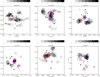 |
Fig. B.1. Selected high density regions for CARLAJ0958-2904 at z = 1.392, CARLAJ0116-2052 at z = 1.425, CARLAJ1103+3449 at z = 1.444, CARLAJ1131-2705 at z = 1.446, CARLAJ2355-0002 at z = 1.49, and CARLAJ1129+0951 at z = 1.528. Passive and active galaxies are shown in red and blue, respectively. We use pink when we cannot separate passive and active galaxies, either because the cluster was not observed in four bandpasses or because the galaxy was not detected in one of the four bandpasses. The ETGs are shown as circles. LTG are shown as squares (disks) and diamonds (irregulars). The cluster spectroscopic members are marked by a small yellow circle; when they are black they are not included in our magnitude, colour and spatial selection, but are shown to better explain our overdensity selection. The RLQ and HzRG are shown as stars and triangles, respectively. |
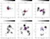 |
Fig. B.2. Selected high-density regions for CARLAJ1753+6310 at z = 1.582, CARLAJ1052+0806 densitymap at z = 1.646, CARLAJ1300+4009 at z = 1.675, CARLAJ2227-2705 at z = 1.692, CARLAJ1510+5958 at z = 1.725, and CARLAJ1018+0530 at z = 1.952 (two selected regions). The symbols are the same as in Fig. B.1. |
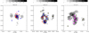 |
Fig. B.3. Selected high-density regions for CARLAJ0800+4029 at z = 1.986, CARLAJ2039-2514 at z = 1.999 (two selected regions), and CARLAJ1017+6116 at z = 2.801. The symbols are the same as in Fig. B.1. |
CARLAJ1358+5752 at z = 1.368: the AGN is close to the highest peak. There are other three peaks. One of these last two is only partially covered by the HST image and another visually seems to be an extension of the second peak. We focus our analysis on the first two peaks, at S/Nc = 17 and 15.
CARLAJ0958-2904 at z = 1.392: the AGN is close to one of the three highest peaks, all with similar S/N, S/Nc = 6, and we center our region on the AGN. This is the structure in which we expect more contamination, with ∼28% being field galaxies.
CARLAJ0116-2052 at z = 1.425: the AGN is within 0.5′ from the highest S/N peak, S/Nc = 16. We concentrate only on the region centered around the highest S/N, because we cannot study in details the second highest S/N region, which is only partially covered by the HST image.
CARLAJ1103+3449 at z = 1.442: The highest S/N peak, is at ∼0.6′ south of the AGN (bottom-right of the S/N map) and the spectroscopically confirmed members are found in other two highest peaks. We don’t have enough information to know if the highest S/N peak is associated with the AGN, and we consider the region centered on the AGN in this analysis, with S/Nc = 10. The AGN host is a star-forming ETG that lies on the field star formation main sequence at the cluster redshift, and we found a large reservoir of molecular gas tens of kiloparsecs to the south of it (Markov et al. 2020).
CARLAJ1131-2705 at z = 1.446: the AGN is close to the highest peak, with S/Nc = 7. The second highest peak is a too much contaminated by field galaxies. We concentrate only on the region centered around the highest S/N peak.
CARLAJ2355-0002 at z = 1.490: the AGN is close to the center of the highest S/N peak at S/Nc = 15. The other peaks have much lower S/N. CARLAJ1129+0951 at z = 1.528: we observe two high peaks. The AGN is within 0.5′ from the highest peak. Both regions host spectroscopically confirmed members. The lowest peak is only partially covered by the HST image and visually appears as an extension of the main overdensity. We focus our analysis on the highest peak, which is S/Nc = 14.
CARLAJ1753+6310 at 1.582: the AGN is close to the center of the highest peak at S/Nc = 23. Noirot et al. (2018) discovered a serendipitous structure with six spectroscopically confirmed members at z = 2.117, superposed to the highest peak. The overdensity around the highest S/N has a regular circular form, and CARLAJ1753+6310 is one of the three clusters that we classified as a highly probable cluster (Noirot et al. 2018). The caveat with this cluster is that we cannot separate the cluster that hosts the AGN from the z = 2.117 structure. However, with this caveat in mind, we make the hypothesis that most of the galaxies in the overdensity belong to the cluster associated to the AGN. Cooke et al. (2016) has shown that the core of this cluster is dominated by passive galaxies.
CARLAJ1052+0806 at z = 1.646: the AGN is at the center of the highest peak, S/Nc = 15. The second-highest peak is overly contaminated by field galaxies. We concentrate only on the region centered around the highest S/N peak.
CARLAJ1300+4009 at z = 1.675: the AGN is close to the highest peak, S/Nc = 15. The other two peaks are at lower S/Nc. One is an extension of the main peak, and the other does not host any spectroscopically confirmed members. We concentrate only on the region centered around the highest S/N peak.
CARLAJ2227-2705 at z = 1.692: the cluster shows several low S/N peaks. The highest peak is at ∼0.9′ north of the AGN. The region around this peak and other minor peaks hosts several spectroscopically confirmed members of the two serendipitous structures discovered by Noirot et al. (2018) at z = 1.357 and z = 1.478. We do not have enough information to associate neither this or the other overdensities to the AGN and the spectroscopically confirmed members. Even if the region centered around the AGN has a S/Nc = 11 and includes several confirmed members, we consider that the contamination from the background and the serendipitous structures is too uncertain to keep this cluster in our analysis.
CARLAJ1510+5958 at z = 1.725: we observe three S/N peaks. The highest density peak (top of the S/N map) is one only partially covered by the HST image. This and another peak also host several spectroscopically confirmed members belonging to the serendipitous discoveries at z = 0.875 and z = 0.977 (Noirot et al. 2018). We concentrate on the third peak (S/Nc = 11) that is also close to the AGN and around which are also found other three spectroscopically confirmed members.
CARLAJ0800+4029 at z = 1.896: the AGN is at the center of the highest peak, S/Nc = 17. There are other overdensities but they are too much contaminated by field galaxies. We concentrate only on the region centered around the highest S/N peak.
CARLAJ1018+0530 at z = 1.952: we observe three high S/N peaks. The AGN is closest to the first highest peak, with S/Nc = 12. We find cluster members in all of these three regions. One of these highest peak (in the S/N map, the peak on the bottom) encompasses a region that is only partially covered by the HST image. We keep only the two highest peaks that are completely covered by HST (S/Nc = 11 and S/Nc = 12) for this cluster, which might be a multiple cluster structure. These regions correspond to the regions discussed in Noirot et al. (2018), where we point out that there is a concentration of bright continuum-only sources in a region northeast of the AGN. This corresponds to our second overdensity, and it shows potential intracluster light. Narrow-band imaging available for this field permits us to derive photometric redshifts that are consistent with the AGN redshifts (Werner et al., in prep.).
CARLAJ2039-2514 at z = 1.999: the region with the highest S/N is ∼0.7′ north of the AGN. The first two highest peaks are within 30″, and the AGN is close to the third highest peak. We selected two regions, centered on the highest peak (S/Nc = 10) and the third peak (S/Nc = 8). This cluster presents a clearly defined colour-magnitude relation (Noirot et al. 2016) and it might be an extended multi-peak structure.
CARLAJ1017+6116 at z = 2.801: the region with the highest S/Nc is centered at a distance of ∼0.6′ from the AGN. Noirot et al. (2018) discovered a galaxy overdensity around this highest peak, with spectroscopical redshift z = 1.235. The second highest peak, with S/Nc = 14, is close to the AGN and closer to the cluster spectroscopically confirmed members. In this analysis, we exclude the overdensity at z = 1.235 and consider instead the second-highest overdensity associated with the AGN.
Appendix C: Passive and active galaxy selection
In this section, we detail how we arrived at the apparent magnitude colour-colour cuts we used to define passive cluster galaxies (see Sect. 2.7). We also show that rest–frame UVJ diagrams obtained with only our four TPHOT magnitudes are not accurate enough to separate passive galaxies at the redshift of the CARLA clusters.
Throughout this analysis, we use the sSFR from Santini et al. as the ‘true’ sSFR and hereafter we define sSFR–passive galaxies as those with sSFR < 10−9.5 M⊙/year, which characterises the quiescent region at our cluster redshifts (e.g. Whitaker et al. 2014; Leja et al. 2019).
We started with the ‘combined CANDELS catalogue’ (described in Sect. 2.3) and selected those galaxies with IRAC1 < 22.6 mag, (IRAC1 − IRAC2) > − 0.1 mag and at 1 < z < 2. This selection results in 646 galaxies, of which 26 ± 3% have sSFR < 10−9.5 M⊙/year, defined here as passive.
Applying the same magnitude, colour and redshift selection to the TPHOT-CANDELS catalogue, we obtain 147 galaxies, of which 20 ± 4% are passive. Because of the limited statistics from the TPHOT-CANDELS catalogue, we consolidated our analysis by using the ‘combined CANDELS catalogue’ and we scaled our results to the TPHOT photometry using empirical relations.
We use this sample to build UVJ diagrams using CANDELS rest-frame U, V, and J bands from our ‘combined CANDELS catalogue’. The passive region defined by Williams et al. (2009) includes 77 ± 4% of the sSFR–passive galaxies. The contamination of sSFR–active galaxies (hereafter defined as galaxies with sSFR ≥ 10−9.5 M⊙/year) is 12 ± 3%. In addition, we define galaxies that are selected within the passive region defined by Williams et al. (2009) as UVJ–passive. This means that the UVJ–passive sample includes a sample of CANDELS sSFR–passive galaxies that is ∼80% complete and ∼90% pure. Overall, UVJ–passive galaxies are 24 ± 2% of our total selectedpg galaxies.
We then derived new rest-frame U, V, and J-band magnitudes by running the software EAZY (Brammer et al. 2008) on our ‘TPHOT-CANDELS catalogue’, fixing the galaxy redshifts to CANDELS spectroscopic redshifts, and using the same templates as those used by the CANDELS collaboration in Fang et al. (2018) (Dave Kocevski’s private communication). When deriving the U, V and J-band in this way (i.e. with four TPHOT bandpasses), our UVJ–passive sample is ∼65% complete and ∼80% pure. Thus, we can consider that our TPHOT bandpasses do not permit us a reasonable estimation of the galaxy spectral energy distribution that could be used to derive rest-frame U, V, and J-band magnitudes.
Therefore, we used our ‘combined CANDELS catalogue’ to derive a linear relation between rest-frame U, V, and J bandpasses and apparent magnitudes of our observed bands, and we built the equivalent of Williams et al.’s regions in the CANDELS apparent i775H160IRAC1 diagram. Using this empirical conversion and iterating to optimise for both completeness and purity, we find an optimal passive galaxy region defined by:
as shown in (Fig. C.1). This colour-colour cut results in a passive galaxy sample that is ∼85% complete and pure for galaxies at 1 < z < 2. These results show that a selection of passive/active galaxies based on apparent CANDELS magnitudes in the redshift range 1 < z < 2 is equivalent to a UVJ selection using the region adopted in Williams et al. using published CANDELS U, V, and J-band magnitudes. This apparent magnitude selection gives much better passive galaxy selection than the use of rest-frame UVJ diagrams obtained using our four TPHOT bandpasses.
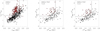 |
Fig. C.1. Passive galaxy selection. Left: Passive galaxy selection using Guo et al. (2013)’s photometry of the 600 galaxies selected from the ‘combined CANDELS catalogue’ at 1 < z < 2. The empty red circles show galaxies with Santini et al. (2015) sSFR < 10−9.5 M⊙/year. The lines show the optimised passive galaxy regions at 1 < z < 2 obtained by using published CANDELS colours from Guo et al. (2013) and similar to the Williams et al. (2009)’s UVJ diagram region. At our survey redshifts, these apparent magnitudes permit us to select in a very similar way as the Williams et al. (2009)’s UVJ diagram region. Middle: Passive galaxy selection at 1 < z < 2, using the TPHOT photometry modified to ACAM depth and filter response. Right: Passive galaxy selection at 1 < z < 2, using the TPHOT photometry modified to GMOS depth and filter response. The empty red circles show galaxies with Santini et al. (2015) sSFR < 10−9.5 M⊙/year. |
We also explored a passive region selection within a simpler two line cut, as implemented in other works (e.g. Ilbert et al. 2013; van der Wel et al. 2014), but we found no significant difference, so we limited our analysis to the three-line passive region.
The last step was to adapt these colours to take into account the filter transmissions of the ground-based ACAM and GMOS i-band and ISAAC z-bands of the CARLA data. Using the ‘TPHOT-CANDELS catalogue’, we derived a linear relation between the CANDELS rest-frame U, V, and J bandpasses and TPHOT apparent magnitudes, and built the equivalent of the regions from Williams et al. in the apparent  diagram. Then we optimised the parameters of the passive galaxy empirical regions by changing the four variables a, b, c, d in the relations:
  ,
,  b and
b and  to optimise the completeness and purity of passive galaxies in the selected region.
The optimal choice of parameters for clusters observed with ACAM is:
whilst for clusters observed with GMOS, the following parameters are used:
These regions can be seen in Fig. C.1. Both selections result in a purity of ∼80%. The ACAM selection results in a completeness of 80%, whereas for the clusters with GMOS data the completeness increases to ∼90%. The active galaxy sample is ∼95% complete and pure in both selections.
At 1.5 ≲ z ≲ 2, the i-band corresponds to the rest frame NUV–band and the z-band to the rest frame U–band. We studied the difference in the passive galaxy sample completeness and purity when using the z-band instead of the i-band.
Using the same techniques as above, but limiting the galaxy sample to those in the redshift range 1.5 < z < 2, we define a passive region through:

This selection, seen in Fig. C.2, results in a passive sample completeness and purity of ∼85%. The active galaxy sample is ∼95% complete and pure.
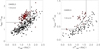 |
Fig. C.2. Passive galaxy selection. Left: Passive galaxy selection using CANDELS photometry. Right: Passive galaxy selection using our TPHOT photometry. Details are the same as Fig. C.1, but using the ISAAC z-band instead of the i-band. |
Again, we use the same techniques as above with the TPHOT-derived photometry, to transform these relations to our ISAAC z-band observation depth and filter response. Our optimal passive region is defined by:
This region is shown in Fig. C.2, and it selects a passive sample that has a completeness and purity of ∼85%. The active galaxy sample is ∼95% complete and pure.
To confirm the completeness and purity of our cluster passive or active selection obtained above, we used our CARLA SFR and mass measurements to calculate the sSFR for the spectroscopically confirmed members in our clusters from Noirot et al. (2018); among them, there are 79 that have SFR measurements and that were detected in all the bandpasses in which their cluster was observed. We measured the sSFR using the SFRs from Noirot et al. (2018) and galaxy masses estimated in this work (only for galaxies detected in IRAC1), resulting in sSFR measurements for 54 galaxies. Hα SFR are available for 40 of these galaxies, and we use O[III] SFR measurements when the Hα flux was not measured. Only 47 galaxies of the 54 were also observed in the i-band or z-band imaging necessary to separate active from passive galaxies using the colour-colour diagrams obtained in this appendix. The passive galaxy selection obtained using this last sample is ∼80% complete (∼80% of the colour-colour galaxies selected as passive have log(sSFR) < − 9.5 [yr−1] at ∼2σ) and pure (∼20% of the colour-colour galaxies selected as passive have log(sSFR) > − 9.5 [yr−1] at ∼2σ). Our sample of galaxies that have been selected as active is also ∼80% complete and pure. With these low numbers, we cannot reach firm statistical conclusions about the completeness and purity of our colour-selected passive sample. However, our CARLA spectroscopically confirmed member passive selection is consistent with the completeness and purity of ∼80 − 85% that we estimated in this appendix using CANDELS catalogues. We note that in the main text, we dropped the prefix "TP" for the TPHOT magnitudes in Figure 4 and after Sect. 2.7.
Appendix D: Fractions as a function of redshift and density contrast
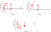 |
Fig. D.1. ETG, passive, and merger galaxy fractions as a function of redshift. The grey region shows the ±1 σ range of the CANDELS fractions. All the fractions that we considered in this work do not show evolution with redshift. We were not able to separate passive and active galaxies in the cluster at z = 2.8. We did not observe any significant correlations. |
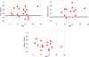 |
Fig. D.2. ETG, passive, and merger galaxy fractions as a function of S/N (as a proxy for density contrast; see text). The grey region shows the ±1 σ range of the CANDELS fractions. We do not observe any significant correlations. |
All Tables
CARLA confirmed cluster sample ground-based observations from Cooke et al. (2015).
CANDELS mass calibration, showing the linear coefficients found for the following relations: Log10(M*) = a + b × (IRAC1) for the CANDELS combined catalogue (CC) and the TPHOT-CANDELS catalogue (TCC), and the scatter around these relations σMC.
CARLA-selected spectroscopically confirmed member classification as passive and active galaxies in this paper.
Corrected fractions of passive galaxies, ETGs, and mergers, and the minimum, maximum, and median ΣN and galaxy stellar mass .
All Figures
|
Fig. 1. Selected high-density regions for CARLAJ1358+5752 at z = 1.368. Passive and active galaxies are shown in red and blue, respectively. ETGs are shown as circles. LTG are shown as squares (disks) and diamonds (irregulars). The cluster spectroscopic members are marked by a small yellow circle, when they are black they are not included in our magnitude, colour and spatial selection but are shown to better explain our overdensity selection. The RLQ is shown as a star. The bar shows S/N levels. |
| In the text | |
|
Fig. 2. Galaxy stellar mass distribution within the cluster overdensities in the redshift range 1.3 < z < 1.6 (continuous line), 1.6 < z < 2.1 (dashed line), and z = 2.8 (dot-dashed line). The three distributions are consistent. |
| In the text | |
|
Fig. 3. Total stellar mass within each overdensity of the CARLA clusters in the redshift range of 1.3 < z < 1.6 (continuous line), and 1.6 < z < 3 (dashed line). These stellar masses roughly correspond to a total halo mass of |
| In the text | |
|
Fig. 4. Cluster colour-colour diagrams. Left: All clusters observed with ACAM. Middle: all clusters observed with GMOS. Right: CARLAJ2039-2514, observed with ISAAC. The continuous lines limit the regions that separate passive from active galaxies. Passive and active galaxies are shown in red and blue, respectively. ETGs are shown as circles. Disks and Irregular galaxies are shown as squares and diamonds, respectively. The cluster spectroscopic members show a yellow dot at the center. The RLQ and HzRG are shown as yellow stars and triangles, respectively, and have spectroscopic redshift even if we do not mark them with a dot. The other AGN have colours that are not included in the plots. The crosses on the upper left are the average colour errors. |
| In the text | |
|
Fig. 5. Passive galaxy fractions as a function of environment. Left: Our entire sample. Right: passive fractions in two redshift bins: 1.3 < z < 1.6 (orange circles) and 1.6 < z < 2 (yellow circles). The grey region shows the ±1 σ range of the CANDELS passive fraction. We observe a significant passive-density relation up to z ∼ 2. |
| In the text | |
|
Fig. 6. ETG galaxy fractions as a function of environment. Left: Our entire sample. Right: ETG fractions in two redshift bins: 1.3 < z < 1.6 (magenta circles) and 1.6 < z < 2.8 (pink circles). We also show with two black circles the fraction for CARLAJ1017+6116 at z = 2.8. The small grey circles and error bars and the dashed line show the morphology-density relation at z ∼ 1 from Postman et al. (2005) and at lower redshift from Dressler (1980). The grey region shows the ±1 σ range of the CANDELS ETG fraction. We observe a significant morphology-density relation up to z ∼ 2. The cluster at z = 2.8 shows a similar fraction of ETGs as in the other clusters, however, one cluster does not provide enough statistics to confirm that the morphology-density relation is already in place at z ∼ 3. In fact, ETG fractions are correlated with environment and increase from high to lower redshift in the intermediate dense regions. |
| In the text | |
|
Fig. 7. ETG galaxy fractions as a function of environment. Details are the same as in Fig. 6, excluding the cluster CARLAJ0800+4029, which shows an high percentage of mergers in its densest regions. We observe a significant morphology-density relation up to z ∼ 2. The ETG fractions drop in the last bin, which is observed in the entire sample (see Fig. 6), is mitigated. This means that the mergers in the high density regions in CARLAJ0800+4029 were dominating the ETG fraction drop observed when including this cluster in the analysis. |
| In the text | |
|
Fig. 8. ETG (left) and passive (right) galaxy fractions as a function of environment. Details are the same as in the right panels of Fig. 5 and Fig. 7, excluding the cluster CARLAJ0800+4029, and separating the z ∼ 2 clusters from the others at z < 1.9. This shows that the relations holds at z ∼ 2. |
| In the text | |
|
Fig. 9. ETG and passive galaxy fractions as a function of global environment defined as total galaxy stellar mass in the overdensity. The grey region shows the ±1σ range of the CANDELS fractions. |
| In the text | |
|
Fig. 10. ETG and passive galaxy fractions as a function of mass in two redshift bins: 1.3 < z < 1.6 and z > 1.6. Symbol colours are the same as in Fig. 5. The grey region shows the ±1σ range of the CANDELS fractions. The ETG and passive fractions mildly increase with increasing mass. |
| In the text | |
|
Fig. 11. ETG and passive galaxy fractions as a function of galaxy surface density in two mass bins: |
| In the text | |
|
Fig. 12. Merger fractions as a function of environment. Top left: Our entire sample. Top right: Merger fractions in two redshift bins: 1.3 < z < 1.6 (dark blue circles) and 1.6 < z < 2.8 (light blue circles). Bottom: Merger fractions as a function of galaxy stellar mass. The grey region shows the ±1 σ range of the CANDELS merger fraction. The merger fraction in our cluster sample is significantly higher than in CANDELS and shows a moderate correlation with environment and mass. |
| In the text | |
|
Fig. 13. Morphology of the eight central HzRG. They all show possible interactions and tidal arms. The radio source in CARLAJ2355–0002 has been discussed in Noirot et al. (2018). |
| In the text | |
|
Fig. 14. Morphology of the spectroscopically confirmed cluster memberss. Left: Morphology class distribution of the 107 spectroscopically confirmed cluster members from Noirot et al. (2018), shown on the left. The classes are: Disk (1), Spheroid (2), Irregular (3), Compact (4), Unclassifiable (5). Most of the members are disks, however there are large percentages of star-forming spheroids and compact galaxies. Right: Morphology class distribution of the members that have ground-based photometry is shown on the right. The blue and red lined histograms correspond to active and passive galaxies, respectively. The passive LTG are galaxies with star formation rates below the field main sequence. |
| In the text | |
|
Fig. B.1. Selected high density regions for CARLAJ0958-2904 at z = 1.392, CARLAJ0116-2052 at z = 1.425, CARLAJ1103+3449 at z = 1.444, CARLAJ1131-2705 at z = 1.446, CARLAJ2355-0002 at z = 1.49, and CARLAJ1129+0951 at z = 1.528. Passive and active galaxies are shown in red and blue, respectively. We use pink when we cannot separate passive and active galaxies, either because the cluster was not observed in four bandpasses or because the galaxy was not detected in one of the four bandpasses. The ETGs are shown as circles. LTG are shown as squares (disks) and diamonds (irregulars). The cluster spectroscopic members are marked by a small yellow circle; when they are black they are not included in our magnitude, colour and spatial selection, but are shown to better explain our overdensity selection. The RLQ and HzRG are shown as stars and triangles, respectively. |
| In the text | |
|
Fig. B.2. Selected high-density regions for CARLAJ1753+6310 at z = 1.582, CARLAJ1052+0806 densitymap at z = 1.646, CARLAJ1300+4009 at z = 1.675, CARLAJ2227-2705 at z = 1.692, CARLAJ1510+5958 at z = 1.725, and CARLAJ1018+0530 at z = 1.952 (two selected regions). The symbols are the same as in Fig. B.1. |
| In the text | |
|
Fig. B.3. Selected high-density regions for CARLAJ0800+4029 at z = 1.986, CARLAJ2039-2514 at z = 1.999 (two selected regions), and CARLAJ1017+6116 at z = 2.801. The symbols are the same as in Fig. B.1. |
| In the text | |
|
Fig. C.1. Passive galaxy selection. Left: Passive galaxy selection using Guo et al. (2013)’s photometry of the 600 galaxies selected from the ‘combined CANDELS catalogue’ at 1 < z < 2. The empty red circles show galaxies with Santini et al. (2015) sSFR < 10−9.5 M⊙/year. The lines show the optimised passive galaxy regions at 1 < z < 2 obtained by using published CANDELS colours from Guo et al. (2013) and similar to the Williams et al. (2009)’s UVJ diagram region. At our survey redshifts, these apparent magnitudes permit us to select in a very similar way as the Williams et al. (2009)’s UVJ diagram region. Middle: Passive galaxy selection at 1 < z < 2, using the TPHOT photometry modified to ACAM depth and filter response. Right: Passive galaxy selection at 1 < z < 2, using the TPHOT photometry modified to GMOS depth and filter response. The empty red circles show galaxies with Santini et al. (2015) sSFR < 10−9.5 M⊙/year. |
| In the text | |
|
Fig. C.2. Passive galaxy selection. Left: Passive galaxy selection using CANDELS photometry. Right: Passive galaxy selection using our TPHOT photometry. Details are the same as Fig. C.1, but using the ISAAC z-band instead of the i-band. |
| In the text | |
|
Fig. D.1. ETG, passive, and merger galaxy fractions as a function of redshift. The grey region shows the ±1 σ range of the CANDELS fractions. All the fractions that we considered in this work do not show evolution with redshift. We were not able to separate passive and active galaxies in the cluster at z = 2.8. We did not observe any significant correlations. |
| In the text | |
|
Fig. D.2. ETG, passive, and merger galaxy fractions as a function of S/N (as a proxy for density contrast; see text). The grey region shows the ±1 σ range of the CANDELS fractions. We do not observe any significant correlations. |
| In the text | |
Current usage metrics show cumulative count of Article Views (full-text article views including HTML views, PDF and ePub downloads, according to the available data) and Abstracts Views on Vision4Press platform.
Data correspond to usage on the plateform after 2015. The current usage metrics is available 48-96 hours after online publication and is updated daily on week days.
Initial download of the metrics may take a while.