| Issue |
A&A
Volume 641, September 2020
|
|
|---|---|---|
| Article Number | A151 | |
| Number of page(s) | 11 | |
| Section | Extragalactic astronomy | |
| DOI | https://doi.org/10.1051/0004-6361/202037660 | |
| Published online | 23 September 2020 | |
Molecular gas in the central region of NGC 7213⋆
1
Dipartimento di Astronomia, Università degli Studi di Bologna, Via Gobetti 93/2, 40129 Bologna, Italy
e-mail: francesc.salvestrin2@unibo.it
2
INAF – Osservatorio di Astrofisica e Scienza dello Spazio di Bologna, Via Gobetti 93/3, 40129 Bologna, Italy
3
INAF – Istituto di Radioastronomia & Italian ALMA Regional Centre, Via P. Gobetti 101, 40129 Bologna, Italy
4
ESO, Karl-Schwarzschild-Str. 2, 85748 Garching bei München, Germany
Received:
4
February
2020
Accepted:
4
July
2020
We present a multi-wavelength study (from X-ray to mm) of the nearby low-luminosity active galactic nucleus NGC 7213. We combine the information from the different bands to characterise the source in terms of contribution from the AGN and the host-galaxy interstellar medium. This approach allows us to provide a coherent picture of the role of the AGN and its impact, if any, on the star formation and molecular gas properties of the host galaxy. We focused our study on archival ALMA Cycle 1 observations, where the CO(2–1) emission line has been used as a tracer of the molecular gas. Using the 3DBAROLO code on ALMA data, we performed the modelling of the molecular gas kinematics traced by the CO(2–1) emission, finding a rotationally dominated pattern. The molecular gas mass of the host galaxy was estimated from the integrated CO(2–1) emission line obtained with APEX data, assuming an αCO conversion factor. Had we used the ALMA data, we would have underestimated the gas masses by a factor ∼3, given the filtering out of the large-scale emission in interferometric observations. We also performed a complete X-ray spectral analysis on archival observations, revealing a relatively faint and unobscured AGN. The AGN proved to be too faint to significantly affect the properties of the host galaxy, such as star formation activity and molecular gas kinematics and distribution.
Key words: galaxies: ISM / galaxies: Seyfert / galaxies: spiral / galaxies: active / X-rays: galaxies
The reduced data cubes are only available at the CDS via anonymous ftp to cdsarc.u-strasbg.fr (130.79.128.5) or via http://cdsarc.u-strasbg.fr/viz-bin/cat/J/A+A/641/A151
© ESO 2020
1. Introduction
Active galactic nuclei (AGN) are thought to play a key role in regulating a host galaxy’s star formation (SF). The accretion of matter onto the central supermassive black hole (SMBH) is responsible for injecting energy in the circum-nuclear region, providing feedback to its host galaxy and the interstellar medium (ISM; see, e.g. Fabian 2012; Somerville & Davé 2015, and references therein). For this reason, the SF activity and SMBH properties are believed to be connected, both in high-redshift quasars and in local Seyfert nuclei. AGN f are held responsible for both suppressing the star formation rate (SFR), which constitutes “negative feedback”, or enhancing it through the compression of molecular clouds, which constitutes “positive feedback”.
In this scenario, the molecular gas plays a fundamental role, because it is the main fuel for SF and the more abundant phase of the ISM in the nuclear region. Therefore, studying the properties of the molecular gas in galaxies and the rate at which it is converted into stars (depletion time, tdepl = Mgas/SFR) is crucial to understanding the processes at play in galaxies. If the AGN is able to completely remove or heat the gas, thus preventing it from cooling, we would expect low tdepl values with respect to inactive galaxies with similar stellar masses (M⋆) and SFRs. Indeed, tdepl (0.01 < tdepl < 0.1 Gyr) lower than in normal galaxies with similar SFRs and M⋆ have been found in luminous AGN at high redshift (i.e. z ∼ 1.5−2.5, Kakkad et al. 2017; Brusa et al. 2018; Talia et al. 2018), while in the local Universe, this effect is not completely understood (e.g. García-Burillo et al. 2014; Casasola et al. 2015; Rosario et al. 2018).
A multi-wavelength approach is necessary to fully characterise the mechanisms regulating the relation between the accretion onto the SMBH and the SF process within its host galaxy. Spatially and spectrally resolved observations, tracing the cold phase of the ISM, are necessary to understanding the impact of the AGN. In fact, if the AGN is present, it can dominate the emission close to the nuclear regions, while at increasing distances from the centre, stellar processes such as supernovae, stellar winds or shocks start dominating. The high spatial resolution and high sensitivity provided by the Atacama Large Millimeter Array (ALMA) are crucial to studying the feeding and feedback processes that could take place on sub-kpc scales, meaning near the nucleus. Coupling this information with a single-dish observation, which is needed to recover the whole content of molecular gas in galaxies, allows us to characterise the properties of the molecular component. This, in combination with the modelling of the spectral energy distribution (SED), using broad-band photometry from the UV/optical to the far infrared (FIR), can allow us to constrain the contributions of stellar processes and the AGN to the global output of the source. Eventually, X-ray observations, especially in the hard band, directly probe the accretion-related emission from the nuclear region, hence the radiating power of the AGN. To obtain a complete picture of the interplay between the AGN and the host-galaxy, it is necessary to coherently combine all the information from the different wavebands.
Gruppioni et al. (2016, hereafter G16) presented the results of a detailed broad-band SED decomposition on a statistically significant sample of local active galaxies, including the emission from stars, dust-reprocessed emission by SF, and AGN dusty torus. The sample consisted of 76 nearby active galaxies (i.e. 36 Seyfert 1, 37 Seyfert 2, and three low-ionisation narrow emission-line regions, LINER) from the complete sample of active and in-active galaxies in the local Universe, selected at 12 μm by Rush et al. (1993). In particular, the 76 sources presented in G16 were selected from the parent sample among the active galaxies based on the availability of mid infrared (MIR) spectra obtained with the IRS spectrograph on the Spitzer telescope. Combining the MIR information with an ancillary collection of photometric data from the optical to the FIR, the analysis of the broad-band SED allowed us to derive M⋆, SFR, Mdust, and the IR luminosity from the AGN and from the SF. To assess whether and to what extent the AGN is able to regulate the host galaxy’s SF, we need to study the properties of the molecular gas, which is the main driver of the SF activity. This goal can be achieved by combining information on the morphology and kinematics of the molecular gas obtained with high-resolution observations in the mm band with the determination of the relative contribution of the AGN to the global outcome of the galaxy (obtained using the SED decomposition and the characterisation of the AGN power through the analysis of the emission in the X-rays).
In this work, we present a test study to show the potential of this multi-waveband method, focusing our attention on one object out of the 76 by G16. The target of this study is NGC 7213, a nearby spiral galaxy showing intermediate properties between a low-luminosity AGN (LLAGN) and a LINER. The source was chosen due to the quality of the available archival observations in different bands, in particular in the X-rays (e.g. NuSTAR and XMM-Newton) to characterise the AGN power, and at mm wavelengths (ALMA and APEX) to trace the molecular gas content and kinematics.
The paper is organised as follows: in Sect. 2, we summarise the multi-waveband properties of the NGC 7213. In Sect. 3, we introduce the data sets that we reduced and analysed in this work. The interpretation of the CO and the continuum mm emission is presented in Sect. 4. Our conclusions and the results are summarised in Sect. 5.
2. NGC 7213
The galaxy NGC 7213 is a nearby (D = 23 Mpc, z = 0.0058) S0 one, which hosts an active nucleus, and was first discovered with the HEAO A-2 satellite (e.g. Marshall et al. 1979). The classification of this source was long debated (e.g. Halpern & Filippenko 1984), and nowadays it is known as an intermediate object – between a LLAGN (with Lbol = 1.7 × 1043 ergs s−1, Emmanoulopoulos et al. 2012) and a LINER (e.g. Starling et al. 2005). The first published optical spectrum by Phillips (1979) suggested the Seyfert 1 classification on the basis of the observed broad Hα emission-line component (with full width at zero intensity ∼13 000 km s−1). They also found that the flux of the Hα was relatively low with respect to what was usually measured in typical Seyfert 1 galaxies, and broad components were very weak or absent in the other observed optical emission lines. Later, Halpern & Filippenko (1984) confirmed the presence of the broad Hα emission line, but the evidence for a low-excitation narrow-line spectrum led to the inclusion of the source in the LINER class.
The X-ray observations confirmed the ambiguous nature of NGC 7213. Archival observations with different X-ray telescopes over several years showed some spectral features in agreement with the Seyfert 1 classification (e.g. an X-ray spectral slope ΓX ∼ 1.8 and no evidence for neutral or ionised absorption features: Bianchi et al. 2008; Lobban et al. 2010; Emmanoulopoulos et al. 2013), while others did not (e.g. the absence of a Compton reflection component, usually observed in local Seyfert 1 galaxies: e.g. Dadina 2008; Ursini et al. 2015).
To complete the multi-band picture of NGC 7213, at radio frequencies the galaxy appears point-like at 3 cm (half power beam width HPBW ≲ 1 arcsec), which was interpreted by Bransford et al. (1998) as either nuclear synchrotron emission or free-free emission. The radio power is P1.4 GHz = 3 × 1029 erg s−1 Hz−1, at least an order of magnitude higher than that of a typical Seyfert, although too low for a radio-loud classification (e.g. Blank et al. 2005). The compactness of the radio emission was also later confirmed by Murphy et al. (2010), who observed NGC 7213 with ATCA at higher frequencies (5, 8, and 20 GHz; see also Bell et al. 2011).
3. Multi-waveband data
In this work, we completed the multi-band picture of NGC 7213 by providing a new and coherent modelling of the most relevant data to describe the overall emission of the source in the X-rays over a broad energy range (including the hard-X data from NuSTAR) and the analysis of sub-mm/mm single-dish (APEX) and interferometric (ALMA) observations. The X-ray data analysis aims to provide an accurate estimation of the accretion power, while the study of the high spatial resolution of the ALMA data is used to characterise the morphology and kinematics of the molecular gas. Finally, the single-dish APEX observation is used to provide reliable estimates of the integrated CO emission, needed to derive the molecular gas mass content.
3.1. X-ray data
The NGC 7213 galaxy has been observed extensively over the last 20 years in the X-rays using a number of facilities, in both soft and hard bands. We are interested in characterising the nuclear activity of the source in terms of the emitting power of the AGN, meaning the luminosity in the 2−10 keV band produced by the primary emission. For this reason, we decided to use the largest band available, combining the information from NuSTAR (nominally, 3−79 keV) with an instrument in the 0.3−10 keV band (i.e. XMM-Newton). We analysed the NuSTAR observation and the one from XMM-Newton with the longer exposure time separately (130 ks: e.g. Emmanoulopoulos et al. 2013) to obtain a global picture of the properties of the source in terms of the spectral features and continuum emission. We did not combine the NuSTAR and XMM-Newton observations since they were not taken simultaneously, and previous works revealed evidence for minor variability in terms of flux and spectral features in NGC 7213 (e.g. Ursini et al. 2015). Nevertheless, the observed variabilities do not significantly affect the X-ray properties of the source (e.g. Bianchi et al. 2003; Lobban et al. 2010; Emmanoulopoulos et al. 2013).
3.1.1. X-ray data reduction
In this work, we re-analysed and combined the following archival observations from XMM-Newton (ID: 605800301; starting on Nov. 11 2009; texp = 132.5 ks) and NuSTAR (ID: 60001031002; starting on Oct. 05 2014; texp = 101.6 ks). We performed a standard data reduction for each data set using the following dedicated softwares: the Science Analysis Software (SAS) v.16.1.0 for XMM-Newton, the HEASOFT (v. 6.19) distribution for NuSTAR Focal Plane Modules (FPM; NuSTARDAS, NuSTAR Data Analysis Software v1.7.1). During data reduction, we checked the light curves for potential time variability, once flaring-background periods were filtered out. No evidence for significant time variability during the observations was found. For each observation, the source counts were extracted from circular regions centred on the radio position of NGC 7213, provided by the NASA/IPAC Extragalactic Database (NED)1. The adopted apertures were chosen depending on the encircled energy fraction (EEF): 15″ for XMM-Newton (corresponding to 90% of the EEF, which was below 5 keV for both EPIC pn and MOS cameras), and 60″ for NuSTAR (corresponding to the 50% of the EEF on the entire band for both FPM cameras). The corresponding background counts were extracted from regions free from sources, close to the target, with circular apertures similar to those used for the source.
We excluded the energy channels where either calibration issues are known to affect the cameras response, or a high background was present (i.e. signal-to-noise ratio ∼1). In particular, for the XMM-Newton pn and MOS cameras, we excluded the channels corresponding to energies below 0.5 keV due to calibration issues, while above 10 keV the background dominates. Furthermore, the soft band below 2 keV is dominated by thermal emission, associated with the high-energy tail of SF-related emission (e.g. Bianchi et al. 2003, 2008; Starling et al. 2005; Lobban et al. 2010). Since we are not interested in interpreting this emission, we excluded the channels below 2 keV from our analysis. Regarding NuSTAR, as high background affected all the channels above 27 keV and calibration issues affected the channels below 3 keV, these energy intervals were also removed. Both NuSTAR and XMM-Newton data were grouped with a minimum number of 30 counts in each channel bin.
3.1.2. X-ray data analysis
The spectral analysis was performed using the X-Ray Spectral Fitting Package (XSPEC) v. 12.10.0c (Arnaud 1996). All the models presented below include the Galactic absorption (NH = 1.06 × 1020 cm−2; Kalberla et al. 2005). We also included cross-calibration constants to account for different responses between EPIC pn and both MOS cameras in XMM-Newton, and between FPM A and B in NuSTAR. We analysed each data set separately and compared our best-fit models with the literature (e.g. Bianchi et al. 2003 for XMM-Newton, and Ursini et al. 2015 for NuSTAR). This also allowed us to check for any potential variability both in flux and in spectral shape as a function of time, since the observations were taken with a separation of five years.
Starting from the XMM-Newton observation, the simplest model we used was a single power-law, with best-fit spectral index ΓX ∼ 1.65. This represents the primary X-ray emission from the nuclear activity, produced by the inverse Compton of the hot electrons from the corona on the seeds of UV photons produced in the accretion disc. It is the emission we are interested in, since it is strictly associated with the accretion processes onto the SMBH. Clear excesses (up to 5σ) were evident in the ∼6−7 keV energy band. Then, we included, one at a time, three Gaussian lines, with a fixed width of 10 eV. Given their best fit energies (see Table 1), they can be associated with the Fe Kα fluorescence emission line at the rest-frame 6.39 keV, and the ionised Fe XXV and Fe XXVI fluorescence emission lines at the rest-frames 6.7 and 6.97 keV, respectively. We found no evidence for absorption of the primary continuum emission (NH < 1021 cm−2). Since some residuals were present in the soft part of the analysed band (i.e. at ∼2 keV), we included a “mekal” component, which is needed to model the excess likely produced by the diffuse emission from the high-energy tail of SF. In the end, our best fit model consists of a power law, three Gaussian emission lines, and a thermal component. The best fit model (χ2 = 388.4 for 321 degrees of freedom) is shown in the top panel of Fig. 1, and the best fit parameters are presented in Table 1 and are consistent with results in the literature (e.g. Emmanoulopoulos et al. 2013). The flux obtained integrating the primary AGN emission (i.e. the power law) in the rest-frame 2−10 keV is  ergs s−1 cm−2.
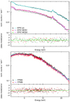 |
Fig. 1. From top to bottom: X-ray spectrum of NGC 7213 obtained with XMM-Newton (EPIC pn, MOS1 and MOS2) and NuSTAR (FPMA and FPMB), as a function of the observed-frame energies. Data and the best fit models for each camera are represented in different colours. In both lower panels, we present the residuals (data minus model) in units of σ. |
Best fit parameters from the X-ray spectral analysis using XMM-Newton and NuSTAR observations, respectively.
Considering the wide energy band (3−27 keV) offered by NuSTAR, we first fit the continuum emission with a single power law. In this case, we obtained a poor fit, with significant residual excess in the ∼6−7 keV band. Given the lower spectral resolution provided by NuSTAR (∼400 eV at 6 keV with respect to ∼150 eV from XMM-Newton), we were not able to constrain both the centroid and the normalisation of the Gaussian lines needed to model the excess in the ∼6−7 keV band. For this reason, we included the Gaussian functions one at a time, setting the energy in correspondence of the best fit obtained with XMM-Newton, then we left the normalisation free to vary (as in Ursini et al. 2015). The primary emission spectral index is significantly higher (ΓX = 1.81 ± 0.02) than the one observed with XMM-Newton, consistently with the literature (Ursini et al. 2015). This is likely due to the wider energy band available to model the primary emission where there are no significant contributions from other components (e.g. the thermal component below 3 keV). Part of the primary emission is usually reflected by the surrounding material around the SMBH, resulting in an excess above 10 keV with respect to the continuum. This reflected component is usually observed in Seyfert 1 galaxies (e.g. Perola et al. 2002), but has never been observed in NGC 7213. We checked for the presence of a reflection component, but the fit was not significantly improved by such inclusion. The best fit is presented in the bottom panel of Fig. 1 (χ2 = 344.2 for 342 degrees of freedom), while the best-fit parameters are shown in Table 1. Integrating the power law over the rest-frame of the 2−10 keV energy band, we estimated a flux of  ergs s−1 cm−2.
Comparing the best fit results between the two observations, variability in both flux and spectral shape is present. The observed variability in terms of flux (the flux measured by XMM-Newton is ∼25% fainter than the that derived by NuSTAR data) is consistent with what is usually observed in AGN, while the different spectral slope (ΓX = 1.64 and 1.81, see Table 1) may be due to the different energy band used for the analysis. In the end, in the X-rays NGC 7213 shows spectral features of a typical low-luminosity Seyfert 1 (i.e. ΓX ∼ 1.8) with no evidence for obscuration, and L2−10 keV = (1.25 ± 0.02)×1042 ergs s−1, using the results from the analysis of the NuSTAR observation. Assuming a bolometric conversion factor of kbol = 9 ± 5 as from Lusso et al. (2012), appropriate for the 2−10 keV luminosity of NGC 7213, we estimate the bolometric luminosity to be Lbol = (1.1 ± 0.6)×1043 ergs s−1, consistent with previous results from literature (e.g. Starling et al. 2005; Emmanoulopoulos et al. 2013). This means that NGC 7213 is accreting at a very low rate, resulting in a rather low fraction of the Eddington luminosity (∼9 × 10⁻⁴, assuming a black hole mass MBH ∼ 108 M⊙, as the one from Woo & Urry 2002). This value is relatively low with respect to typical Seyfert 1 galaxies (a few percent), again stressing the intermediate nature of NGC 7213 between a Seyfert galaxy and a LINER.
3.2. ALMA data
The ALMA observations of NGC 7213 were taken in May 2014 (early science project: 2012.1.00474.S, PI: N. Nagar) at 230 GHz (band 6), in configuration C32-5, including 31 12 m antennas. These observations cover the angular scales in the range of 0.5″ − 25″, corresponding to 60 pc−3 kpc at the redshift of the source, where 0.5″ is the spatial resolution, while 25″ is the field of view (FoV). However, the largest angular scale that was recovered with the adopted antenna configuration is 6.2″, or 750 pc. The spectral setup consisted of three high-resolution spectral windows with 1920 channels of 976.562 kHz in width each, and a low-resolution spectral window of 128 channels of 15.626 MHz in width. Two of the high-resolution spectral windows were centred on the observed frame frequency of the 12CO(2–1) and CS(5–4) emission lines at 229.2 GHz and 243.5 GHz, respectively. The remaining two windows were centred on the sky frequencies at 240.4 GHz and 227.8 GHz, respectively, in order to measure the sub-mm continuum emission.
The data were calibrated using the ALMA calibration scripts, with CASA version 4.5.3. J2056-4714 was observed as bandpass calibrator, J2235-4835 as phase calibrator, while Neptune was used as an amplitude calibrator, assuming the Butler-JPL-Horizons 2012 model. From the calibrated data, continuum and line images were obtained using the CASA task, “clean”. We adopted the natural weighting to get the best signal-to-noise ratio.
3.2.1. The continuum emission
In Fig. 2, the contour levels of the continuum emission (at 235.1 GHz, or 1.28 mm), obtained from the line-free channels in all the four spectral windows, are presented in red. The beam size is 0.48″ × 0.44″ (with a beam position angle of ∼81.1 deg) and a 1σ rms level of 8.9 × 10⁻⁵ Jy beam−1. The emission is clearly produced by a ≲60 pc-sized point-like source. Using the “imfit” task from the CASA software, we fitted the map with an elliptical Gaussian profile. The best fit centroid is consistent (within the uncertainties) with the NGC 7213 radio position provided by the NASA-IPAC Extragalactic Database (NED)2. The “imfit” task provided the continuum flux density, integrating the Gaussian profile, with the corresponding uncertainty: Fν, cont = 40.1 ± 0.1 mJy.
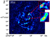 |
Fig. 2. ALMA CO(2–1) integrated intensity image with the continuum emission overlaid in red contours (at 5σ, 10σ, and 50σ levels). The white ellipse in the bottom-left corner represents the synthesised beam of 0.50″ × 0.47″ with a position angle of 73.4 deg. The three interesting regions are magnified in the two boxes: a possible outflow (A) located at the edge of a super bubble (B) and a second potential outflow observed from the PV diagram analysis (C; see Fig. 7). |
3.2.2. The CO(2–1) emission line
The CO(2–1) emission line was extracted from the continuum-subtracted cube of the first spectral window. We used the CO(2–1) frequency at the redshift of z = 0.0058 (NED) as a reference frequency. We used the “clean” task to iteratively clean the dirty image, selecting a natural weighting scheme of the visibilities. We binned the cube to increase the signal-to-noise ratio, requiring a spectral resolution of 10 km s−1. The cleaned image of the CO(2–1) emission line has a synthesised beam of 0.50″ × 0.47″, with a position angle of 73.4 deg and an average 1σ rms of 0.1 mJy beam−1 per channel.
As presented in the integrated intensity map (see Fig. 2), the spatial distribution of the CO line flux follows a spiral-like pattern, which is characterised by a clumpy emission. This can be explained by the combination of the intrinsic clumpy nature of the emitting medium, with the lack of a more diffuse component, which has most likely been resolved because of the extended antenna configuration adopted for the interferometric observation. Using a circular region with a diameter of 25″ (or ∼3 kpc, roughly corresponding to the FoV of the instrument), we measured fCO, ALMA = 112 ± 5 Jy km s−1 as the flux of the CO(2–1) emission line. The uncertainty on the flux density is the quadratic sum of the two main contributions: the rms within the same aperture, and the flux calibration uncertainty (∼5%, as suggested when using Neptune as flux calibrator).
Regarding the morphology, the CO(2–1) emission traces the spiral arms of the galaxy, as can be observed in Fig. 3, where the contours of the CO emission line are superimposed onto an archival HST optical observation (taken with the F606W filter on the WFPC2; Malkan et al. 1998). The molecular gas is clearly co-spatial with the spiral arms, while the size of the narrow-line region, estimated from the [O III] line observed with the FR533N filter on the HST/WFPC2 (Schmitt et al. 2003), is less than 100 pc. This suggests that the CO(2–1) is most likely heated by the stellar activity within the arms rather than the low-luminosity AGN hosted in the centre. This is in agreement with theoretical models (e.g. Obreschkow & Rawlings 2009; Meijerink et al. 2007; Vallini et al. 2019), where the impinging radiation for the low-J transitions like the CO(2–1) mainly comes from the photodissociation regions (PDRs; e.g. Pozzi et al. 2017; Mingozzi et al. 2018) rather than from the X-ray dissociation region (XDR) heated by the central AGN. Indeed, looking at both Figs. 2 and 3, the lack of CO emission at the location of the ALMA continuum emission and a lack of the peak of the optical emission (both indicative of the location of the nucleus) are evident.
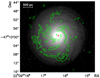 |
Fig. 3. Contour levels of continuum (red) and CO(2–1) line emission (green, at 2σ, 4σ, and 6σ levels) are superimposed on an optical image from the Hubble Space Telescope (HST; F606W filter). The molecular gas follows the same spiral-like pattern as the optical emission. The continuum is produced by a point-like source. |
3.3. APEX data
The APEX observation of the CO(2–1) emission line (at 229.2 GHz sky frequency) was carried out with the PI230 receiver at the Atacama Pathfinder Experiment (APEX; project 0103.F-9311, PI: F. Salvestrini). The need for the single-dish observation was motivated by the potential filtering of the CO emission at intermediate and large scales in the interferometric observations. Indeed, the archival ALMA data were limited by the maximum recoverable scale (MRS; ∼6.2″, or ∼750 pc) of the antenna configuration adopted. This could result in a significant underestimation of the molecular gas content traced by the CO emission. As reported in Sect. 3.2.2, the clumpy morphology observed in the interferometric observation, along with the lack of a fainter diffuse component, supported this hypothesis.
Data reduction was performed using the CLASS program, which is part of the GILDAS3 software. The CO(2–1) emission-line profile is presented in Fig. 4. The spectral resolution requested for the APEX observation (50 km s−1) is sufficient to observe the double-peak structure of the line profile. This profile is generally associated with rotation-dominated motion, in agreement with the results from the kinematical study of the ALMA data that is presented in Sect. 4.2. The integrated CO(2–1) surface brightness was obtained performing a fit using a double Gaussian function to the line profile. The resulting value is ΣCO = 9.6 ± 1.4 K km s−1. The uncertainty on the surface brightness is dominated by the calibration uncertainty, which was conservatively assumed to be 15%, as it has been for similar observations (e.g. Csengeri et al. 2016; Giannetti et al. 2017). To compare this value with the one that we obtained from the ALMA observation, we used the Jy/K conversion factor, which depends on the aperture efficiency of the telescope. In the configuration adopted for our observation (PI230 detector), with Jupiter as a calibrator, the conversion factor is 35 ± 34. Then, fCO, APEX = 340 ± 60 Jy km s−1, meaning ∼3 times the fCO, ALMA reported in Sect. 3.2.2. This implies that the ALMA interferometric observations only recovered about 30% of the CO(2–1) flux density measured with APEX.
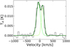 |
Fig. 4. CO(2–1) emission line observed with the PI230 receiver at APEX. On the x-axis, the velocity in km s−1, on the y-axis the antenna temperature in K; the channel width is Δv = 50 km s−1. Two Gaussian functions (in dashed light green lines, while the sum of the two is in dark green) are needed to reproduce the double-peak spectrum profile (in black). A rotation-dominated kinematics is suggested by the double-peaked line profile. |
3.4. SED decomposition
The galaxy NGC 7213 benefits from a detailed SED decomposition performed by G16, which allowed us to disentangle the relative contributions of AGN and SF activity to the global IR outcome of the source, providing a characterisation of the host galaxy in terms of stellar and dust content (M⋆ and Mdust, respectively), and ongoing SF (SFR). Here, we briefly introduce the photometric data collected from the archive and the SED decomposition procedure adopted by G16. The homogenised catalogue of total fluxes, from the UV to the FIR, is presented by G16 (see also their Table A.1: the flux densities are corrected for the aperture and magnitude zero point). In the case of NGC 7213, the photometric data included in the analysis are: the U, B, V, and R bands from de Vaucouleurs et al. (1991); the near-infrared measurements from the catalogue by Jarrett et al. (2000); the IRS spectrum re-binned by Gruppioni et al. (2016) and the photometry by Gallimore et al. (2010) and Moshir et al. (1990) in the MIR; and the FIR photometry by Spinoglio et al. (2002). The adopted SED fitting code was SED3FIT5 (Berta et al. 2013), which reproduces the stellar emission and the emission of the dust heated by the stars and the torus emission simultaneously. The code used the library by Bruzual & Charlot (2003) for the stellar contribution, that of da Cunha et al. (2008) for the IR dust-emission, and the library of smooth AGN tori by Fritz et al. (2006), updated by Feltre et al. (2012). In order to limit the degeneracy among the torus parameters, in G16 the AGN configurations of obscured sources were excluded for NGC 7213 (as supported by optical observations of the source and by the X-ray spectral properties presented in Sect. 3.1.2). The best fit model and the decomposition in the different components is presented in Fig. 5. The host-stellar contribution and the dusty SF dominate over the AGN in the optical bands and in the entire IR band, respectively. While this could appear to be in contrast with the type 1/broad-line nature of the AGN, it is in agreement with the relatively weak nuclear activity observed in NGC 7213 (revealed also through the X-ray spectral analysis reported Sect. 3.1.2).
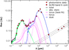 |
Fig. 5. Decomposed SED of NGC 7213, obtained with the SED3FIT code (Berta et al. 2013). Green, pink (continuous line), and blue lines represent the contribution from the extinguished stars, the dusty torus, and the emission reprocessed by dust, respectively, while the black solid curve is the sum of all components (total emission). The red circles are the photometric measurements, from the optical to the radio frequencies (i.e. the ATCA observations at 5, 8, and 20 GHz, not included in the SED decomposition). As explained in Sect. 3.4, the nature of this emission (represented by the red square) is compatible with non-thermal emission produced in the nuclear region, i.e. synchrotron emission. Even considering extreme models (the pink dashed lines), the dusty torus cannot be responsible for the observed emission (red square), since it would be too faint at mm wavelengths (at least two orders of magnitudes fainter). Then, we fitted the three radio-frequency observations by ATCA with a power law, obtaining the best-fit slope represented by the black solid line (the dashed lines correspond to the 1-σ levels). |
4. Interpreting the CO and continuum sub-mm emission
4.1. The point-like continuum
The continuum map at 235.1 GHz (or 1.28 mm) is shown in Fig. 2. Two interpretations are consistent with the point-like nature of the observed continuum: (a) nuclear synchrotron emission, (b) thermal dust emission. The interpretation in point (a), which is the non-thermal emission produced in the very nuclear region, is supported by the compact morphology and the result of the fit presented in Fig. 5. Furthermore, the ALMA continuum emission (represented by a red square, Fig. 5) is consistent with the extrapolation of the relation derived from the radio points including uncertainties. This relation was obtained by fitting a power-law relation (Sν ∝ λα) to the radio flux densities at 5, 8, and 20 GHz (obtained simultaneously at the Australia Telescope Compact Array, ATCA; Murphy et al. 2010). Indeed, the source appears to be point like (i.e. there is no evidence for jets or large-scale structures) at these frequencies. We obtained a slope of α = 0.54 ± 0.03, which is consistent with the slope observed in the case of synchrotron emission. With the current data, we are not able to exclude the contribution from other mechanisms (e.g. free-free emission; see discussion in Ruffa et al. 2018).
Regarding point (b), which is the contribution from thermal emission, we refer to the results of the SED de-composition analysis presented in G16 and briefly introduced in Sect. 3.4. Given the point-like nature of the continuum emission observed with ALMA (shown as a red square in Fig. 5), we conclude that it cannot be associated with the tail of the FIR bump. This possibility is rejected since the FIR bump is expected to be produced by a diffuse dust component, which was not detected in the ALMA observation. Alternatively, it could be associated with the thermal emission from the dusty torus, even if the predicted torus emission at 1.3 mm is significantly lower than the observed flux for the best fit torus template (see the thick pink line in Fig. 5). To test this hypothesis, we also considered extreme torus configurations (pink dashed lines) to maximise the torus contribution to the FIR emission. In particular, we considered torus models with high optical depth (τ = 10) and with the highest outer-to-inner radius ratio (Rmax/Rmin = 300). Since the dust sublimation radius is usually assumed as the inner radius, with a size of ∼pc for a typical AGN luminosity as in the case of NGC 7213 (e.g. Fritz et al. 2006), this corresponds to an outer radius of ∼300 pc. It is important to notice that the “extension” of a typical torus in an intermediate-luminous AGN is below 10 pc, as was observed with ALMA in local active galaxies (e.g. García-Burillo et al. 2014). Having said this, when we also considered these extremely extended torus models, we were not able to reproduce a significant fraction of the continuum emission observed with ALMA. We thus excluded the thermal emission from dust as a major contribution to the observed continuum emission at 1.3 mm.
4.2. Molecular gas kinematics
The spatial resolution provided by ALMA observations allowed us to perform a detailed study of the kinematics of the molecular gas, tracing it from the large scales (e.g. the rotating galactic disc) to the very central regions, where the accretion onto the central SMBH takes place. This kind of study has been successfully performed on large numbers of local Seyfert galaxies (e.g. García-Burillo et al. 2014), and also in galaxies from the same parent sample (e.g. Sabatini et al. 2018). Following a similar approach to that adopted by Sabatini et al. (2018), we used the 3DBAROLO (3D-Based Analysis of Rotating Object via Line Observations) software (Di Teodoro & Fraternali 2015) to model the kinematics of the molecular gas, as traced by the CO(2–1) emission line. The 3DBAROLO code was specifically developed to fit 3D tilted-ring models based on two main assumptions: (i) the material that is responsible for the observed emission has to be contained in a thin disc, and (ii) the kinematic has to be dominated by rotation. The first assumption is generally accepted for local S0 galaxies. Regarding assumption (iii) the ALMA observation of NGC 7213 revealed a rotation-dominated pattern, clearly visible from the velocity map (moment-1 map) of the CO(2–1) emission line (see the central panel of Fig. 6). We fixed the kinematic centre to the centroid of the continuum emission, whose profiles have been fitted (using the “imfit” task from CASA) using an elliptical Gaussian. This is based on the assumption that the nucleus is the centre of the rotation and is responsible for the continuum emission (see Sect. 3.2.1). To reduce the model degeneracies, we set the disc geometry by fixing some parameters. From the data, we set the position angle of the major axis to PAmajor = 330° from north to west. We also fixed the inclination of the disc with respect to the line of sight to i = 30°, as estimated in the literature (e.g. Storchi-Bergmann et al. 1996; Lin et al. 2018). The central velocity of the ALMA data cube has been chosen to be that of the CO(2–1) sky frequency, meaning 229.2 GHz, but we left the systemic velocity (vsys) free to vary in order to account for potential inaccuracies relative to the adopted sky frequency. Given the tradeoff of “holes” and clumpy emission, we preferred the pixel-by-pixel (i.e. “local”) normalisation over the “azimuthal” one (i.e. the azimuthally averaged flux in each ring) in order to account for the non-axial symmetry of the emission, meaning regions with anomalous gas distribution, which could affect the global fit. For the same reason, we allowed 3DBAROLO to perform a smoothing of the input data cube by a factor of 2 of the original beam of the observation (i.e. the data were convolved with an elliptical Gaussian that was twice the size of the original beam), and to cut the smoothed cube at a signal-to-noise ratio of 4. We set the maximum number of radii to eight, separated by 1.5″ or ∼180 pc, excluding the outermost part of the field of view, where 3DBAROLO was not able to fit the model to the faint clumpy emission. To summarise, the free parameters are: the circular velocity, the systemic velocity, and the velocity dispersion.
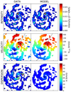 |
Fig. 6. From top to bottom: comparison between the flux, velocity, and velocity dispersion maps obtained from the data (left column) and the best fit model produced by the 3DBAROLO code (right column). Both the data and model have been convolved with an elliptical Gaussian twice the size of the beam of the observation. This smoothing procedure helps the 3DBAROLO in the fitting procedure, especially in the case of clumpy emission as the one analysed here. The grey lines in the central panels represent the direction of the position angle; the same slit was used to extract the position-velocity (PV) diagram on the major axis, as presented in the top panel of Fig. 7. |
At first, we did not include any potential radial velocity components in order to reduce the number of free parameters. Once the best fit model was obtained, meaning the residuals (data minus model) showed no significant evidence for rotational motion, we tested for the presence of a radial velocity component (vrad). We ran the code with this additional free parameter, but its best fit value was consistent with zero. By assuming different values of the PA (PA = 320 ° −340°) and inclination (i = 20 ° −40°) one at a time, we tested the goodness of the fiducial values of the PA and inclination angle. Since the residual clumps proved to be not sensitive to the choices of the assumptions, we preferred the best fit model with PAmajor = 330° and i = 30°. The results from the kinematical analysis are presented in Fig. 6, where the comparison between the model and the data in terms of intensity, velocity, and velocity dispersion maps (zeroth, first, and second moments, respectively) is shown. The model and data (smoothed by a factor of (2) are in excellent agreement. The kinematics of the molecular gas, traced by the CO(2–1) emission line, are clearly dominated by purely circular rotational motions around the nucleus. This is the first successful attempt to model the kinematics of the molecular gas in NGC 7213, thanks to the software 3DBAROLO, which is able to handle the available data, despite the sparse information that limited previous attempts to model the kinematics (e.g. Ramakrishnan et al. 2019). As is clearly visible in Fig. 7, we found that the data cube central velocity was offset by an additional δVsys = 36 ± 10 km s−1. This means that the systemic velocity of the source with respect to our rest frame has to be Vsys = 1716 ± 10 km s−1, which is a mean value between the systemic velocity obtained from the study of the stellar kinematics by Schnorr-Müller et al. (2014), and the results by Ramakrishnan et al. (2019).
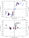 |
Fig. 7. PV diagrams on the major (top panel) and minor (bottom panel) axis, respectively. On the x-axis, the angular distance from the centre of the source along the direction fixed by the angle ϕ is reported. On the right y-axis, the velocity along the line of sight (in km s−1) is shown as it appears in the input data cube. On the left, the velocity along the line of sight (in km s−1) is shown, once the systemic velocity (vsys = 36 ± 10 km s−1) has been subtracted. The data are represented in grey scales with blue contours, while the best fit model is identified by red contours. Upper panel: the blue circles represent the projected best fit rotational velocity at different radial distances from the centre, associated with each ring of the disc. Bottom panel: the signature of the potential outflow associated with Region C (bordered in green; see Sect. 4.3) is clearly visible as an excess of CO emission over 100 km s−1 with an offset of ∼1″ from the centre of the rotation. |
Looking at the lower panels, the velocity dispersion in the best-fit model is ∼10−15 km s−1: values that are expected from a rotation-dominated disc. The highest values of the velocity dispersion (vdisp ∼ 70 km s−1) are not reproduced by the best fit model. The high-dispersion residual clumps proved to be insensitive to our assumptions (e.g. PA, i, vrad), therefore we suggest that the residuals are associated with non-rotational motion, as we discuss in Sect. 4.3.
4.3. Complex structures in the CO emission
The results of the modelling of the gas kinematics presented in Sect. 4.2 pointed out the presence of a few regions where the kinematics are not strictly associated with rotational motion. To investigate the nature of these regions, we used both the position-velocity (PV) diagrams, shown in Fig. 7, and the moment maps (intensity, velocity, and velocity dispersion maps) from Fig. 6. In particular, we focused on three regions, which we named A, B, and C (see Fig. 2) and interpreted as follows:
Region A is an extended emission (of the order of 1.5″ × 2.5″), showing an asymmetric line profile (see Fig. 8). Region B is a possible super bubble, meaning it is a nearly circular void of 0.7″ or 90 pc in diameter, surrounded by likely shocked material. It is located 3.3″ (400 pc) NE of the nucleus. Region C is a likely outflow located 1.4″ (150 pc) SE of the nucleus along the minor axis.
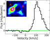 |
Fig. 8. Asymmetric line profile observed in correspondence with the potential outflow in Region A. This emission is likely produced by shocked material. |
Since Region A is located at the edge of the circular void identified as Region B, the former can be interpreted as the emission produced by the shock front impacting on the surrounding medium. However, further observations that successfully recover the CO emission at all scales with good spatial resolutions are needed to validate this hypothesis. The potential outflow in Region C was identified from the PV diagram along the minor axis, presented in the bottom panel of Fig. 7. This emission (Region C), located along one of the spiral arms and observed over 100 km s−1 (corresponding to at least 10 channels), is clearly not consistent with what is expected from a rotation-dominated disc. The interpretation as emission from outflowing gas is supported by the presence, at the same location, of a peak in velocity dispersion associated with a 1.5″ × 1″, or 180 pc × 120 pc region (see the dispersion map in Fig. 6). From the residual of the kinematical modelling, we measured the peak velocity (vmax), the size (ROF), and the flux of the emission associated with the outflow. The flux was used to derive the outflow mass (MOF), following the procedure extensively described in Sect. 4.4. The molecular gas outflow mass was calculated by assuming an αCO = 1.1 M⊙ pc−2 (K km s−1)−1, as for the gas mass from the APEX observation, which is a value similar to the one used in literature (e.g. Cicone et al. 2014; Fiore et al. 2017). Then, we computed the mass-outflow rate (ṀOF) of Region C, assuming a spherical geometry (i.e. ṀOF = 3vmax MOF/ROF). We compared this value (ṀOF ∼ 0.03 ± 0.02 M⊙ yr−1) with the one we expected from the ṀOF − LAGN relation (e.g. Cicone et al. 2014; Fiore et al. 2017), predicting, for Region C, a mass loss ṀOF ∼ 7 − 15 M⊙ yr−1. This prediction is at least two orders of magnitude larger than what we measured, thus suggesting that it is unlikely to be purely AGN driven. Furthermore, the outflow is located relatively far from the low-luminous nucleus of NGC 7213, thus suggesting a dominant contribution from a stellar-like driven mechanism. The same calculation was performed in the case of the potential outflow in Region A, suggesting a stellar-related mechanism powering the molecular wind, given the measured ṀOF ∼ 0.05 ± 0.03 M⊙ yr−1.
4.4. The molecular gas mass
The cold molecular gas mass (Mgas) can be estimated from the luminosity of the CO(1–0), given αCO, the CO-to-H2 mass conversion factor (Mgas = αCO  : see Solomon & Vanden Bout 2005). This relation is widely used in the literature, but (a) we need to extrapolate the CO(1–0) luminosity from our measurements of the CO(2–1) line, and (b) we need to assume an appropriate value for the αCO. Regarding point (a), while at high transition numbers (J > 3) the CO spectral energy distribution (COSLED) strongly depends on the excitation mechanism (i.e. SFR, AGN, shocks: Meijerink et al. 2007; Pozzi et al. 2017; Mingozzi et al. 2018) and the ISM physical properties (i.e. density, geometry: see Hollenbach & Tielens 1999; Vallini et al. 2019), at lower-J the COSLED shape is rather uniform, tracing the cold and diffuse phase (e.g. Narayanan & Krumholz 2014), with a typical CO(2–1)-to-CO(1–0) flux ratio ∼3 (e.g. Papadopoulos et al. 2012). We therefore assumed fCO(2−1)/fCO(1−0) = 3, and we applied this factor to the CO(2–1) emission-line flux observed with APEX. We did not take into account the CO(2–1) line flux observed with ALMA, because, as explained in Sect. 3.3, it represents only a fraction of the flux observed with APEX. This difference is likely due to the filtering out of the large-scale emission in the interferometric observation, hence considering that the CO flux measured with ALMA could result in a significant underestimate of Mgas.
Then, we calculated  following Carilli & Walter (2013):
where SlineΔv is the flux of the emission line in Jy km s−1, assuming for the CO(1–0) line width the same as measured for the CO(2–1), DL is the luminosity distance in Mpc, νrest the rest-frame frequency of the line in GHz. We obtained  K km s−1 pc2. To check whether the CO emission recovered by APEX observation is representative of the expected molecular gas emission from NGC 7213, we used the relation log(
 ) = (0.73 ± 0.03)log(LIR) + (1.24 ± 0.04) (e.g. Carilli & Walter 2013), which relates the CO and the IR luminosity (LIR). A negligible contribution from the AGN in the FIR was accurately assumed (see also Fig. 5). Using the SF-related IR luminosity provided by G16 (LIR = (1.0 ± 0.3)×1010 L⊙), we obtained
  K km s−1 pc2. The CO luminosity obtained with APEX is roughly a factor of ∼2 smaller than the one extrapolated from the IR emission, however, the two values are consistent within the uncertainties. This suggests that the CO luminosity collected within the APEX aperture (25″, or ∼3 kpc) is almost representative of the CO emission from the entire galaxy, hence of the entire molecular gas content. Therefore, for the estimate of Mgas presented in this section, we used the CO(1–0) luminosity from APEX.
The choice of an appropriate αCO factor (point b) depends on the ISM conditions. For example, αCO has a strong dependance on the metallicity (metal-poor galaxies show αCO up to a factor of 5−10 higher than Milky Way-like galaxies, see Fig. 9 from Bolatto et al. 2013) and a relatively less significant dependance on the compactness/starburstness of the sources (see Fig. 12 from Bolatto et al. 2013). Since we cannot derive the metallicity for NGC 7213 from the optical spectrum, we assume it to be solar like. For active and luminous IR galaxies, the generally adopted αCO values are in the range ∼0.3−2.5 M⊙ pc−2 (K km s−1)−1 (see also Downes & Solomon 1998; Papadopoulos et al. 2012). For NGC 7213, we assumed αCO = 1.1 M⊙ pc−2 (K km s−1)−1, which is used for the nuclear regions of metal-rich galaxies (e.g. Sandstrom et al. 2013; Rosario et al. 2018). Thus, we compared our result with literature works on local active galaxies showing similar properties to NGC 7213 (e.g. Pozzi et al. 2017; Rosario et al. 2018). Based on the above assumptions, the molecular gas mass derived from the flux estimate obtained with APEX is Mgas = (2.0 ± 0.3)×108 M⊙.
Given Mgas, we estimated the depletion time, as tdepl = Mgas/SFR. Since the SFR provided by G16 (SFR = 1.0 ± 0.1 M⊙ yr−1) is referred to the entire galaxy, while the APEX aperture covers ∼25″ (or ∼3 kpc), we needed to scale down the SFR. This is necessary since the two measurements were obtained with different apertures and because the SF surface brightness in NGC 7213 appeared to be extended beyond the central region (Diamond-Stanic & Rieke 2012). We considered the PACS observation at 70 μm from the Herschel telescope (PSF FWHM ∼ 5.6″), where the contribution from the central AGN should be less important to the global IR outcome with respect to the relative nuclear contribution at shorter wavelengths, as suggested by the result of the SED decomposition analysis presented in Fig. 5 and from the low-luminosity nature of NGC 7213 presented in this work. The extended IR emission at 70 μm is almost entirely produced by the SF activity, hence it can be used as a proxy of the SFR surface brightness. We found the flux ratio within the entire galaxy (Ftot) and the APEX aperture (25″; F25″) to be Ftot/F25″ = 2.0 ± 0.3. Eventually, assuming the scaled SFR, we measured a depletion time of tdepl = 0.4 ± 0.1 Gyr. This value is consistent with what is observed in the local Universe in objects with similar properties in terms of M⋆ and SFR (0.1 < tdepl < few Gyr; e.g. Rosario et al. 2018), but larger than what is observed at high redshift (0.01 < tdepl < 0.1 Gyr; e.g. Brusa et al. 2018; Kakkad et al. 2017; Talia et al. 2018). The observed difference in tdepl between high- and low-redshift samples is most likely due to the stronger SF and AGN activity at the cosmic noon (e.g. Madau & Dickinson 2014), resulting in shorter timescales for the gas consumption.
5. Discussion and conclusions
In this work, we present a multi-wavelength approach to the study of NGC 7213, a low-luminosity AGN with a wealth of multi-wavelength observations. The source was selected from the sample presented by G16, on the basis of the quality of the available archival observations in the X-rays and at mm wavelengths. The multi-band information helps us to draw a more complete picture of the physical processes in this object, the different phases of the ISM in the host galaxy, and the role of the AGN. To this aim, we performed a spectral analysis of X-ray archival observations to study the accretion-related emission in terms of power and spectral shape. We also combined the high-sensitivity and high-spectral resolution from ALMA, which is crucial to tracing the molecular gas kinematics down to sub-kpc scales, with the spatially integrated information provided by APEX, to estimate the molecular gas content. The main results of this work can be summarised as follows:
-
Our re-analysis of archival XMM-Newton and NuSTAR observations allowed us to properly characterise the central engine in terms of spectral shape and power over the 2−27 keV energy band. The results of the X-ray spectral analysis (i.e. ΓX = 1.81 ± 0.02 and
 ergs s−1 cm−2, derived from NuSTAR observations due to the wide energy band covered: see Table 1) support the presence of an unobscured AGN in the centre of NGC 7213, which is in agreement with its classification as a Seyfert 1 galaxy, based on the optical broad-line features. However, the relatively low luminosity of the source in the X-rays (L2−10 keV ∼ 1 × 1042 ergs s−1) suggests a low accretion rate that is far below the Eddington limit. The energetics related to the nuclear activity of NGC 7213 place the source in an intermediate stage between a typical Seyfert galaxy and a LINER.
 -
Using 3DBAROLO on the ALMA data of the CO(2–1) emission, we obtained the first model of the molecular gas kinematics in the central regions of NGC 7213. The best-fit model well reproduces the velocity fields, which are dominated by a rotational pattern. From the residuals we found no evidence for non-rotationally dominated motion in the central region (i.e. ≲60 pc from the nucleus). This means that the SMBH hosted in NGC 7213 cannot significantly affect the motion of the molecular gas traced by the CO(2–1) at the scales recovered in the available observation, since there is no evidence for nuclear inflows or molecular gas streaming feeding the AGN.
-
The study of the CO emission-line data cube showed some evidence for two potential outflows, located within 500 pc of the nucleus. Region A is located at the edge of a circular void, and it is likely a super-bubble. The evidence for Region C came from the PV-diagram analysis and is located along one of the spiral arms. Given the sizes and the location of both, they are more likely powered by stellar activity, rather than by the AGN, but better data are needed to confirm this hypothesis.
-
The continuum emission at 235.1 GHz (1.28 mm) is produced by a point-like source. Based on an SED analysis, we concluded that the most reasonable interpretation is the continuum being produced through synchrotron radiation in the nuclear region, in agreement with the extrapolation of the ATCA observations at longer wavelengths.
-
The molecular gas mass of NGC 7213 is Mgas = (2.0 ± 0.3)×108 M⊙, which was obtained by converting the CO luminosity observed with APEX. We underline how the ALMA observation would have underestimated the gas mass by a factor of ∼3, given the filtering out of the large-scale emission in interferometric observations. We estimate a depletion time of tdepl = 0.4 ± 0.1 Gyr, which is consistent with what is observed in local moderately luminous Seyfert galaxies (e.g. Rosario et al. 2018). This suggests a negligible, if any, AGN impact on the host galaxy’s SF activity.
The proposed approach allowed us to combine the available multi-wavelength information to obtain a coherent picture of the source in terms of both AGN activity and host galaxy ISM properties. In the case of NGC 7213, the accretion-related emission from the AGN is rather weak, and thus unable to significantly impact the molecular gas content and distribution of the galaxy, and hence to influence the SF activity, as suggested by the depletion time. Given the results of our study, NGC 7213 can be classified as an LLAGN, showing an intermediate nature between a Seyfert 1 galaxy and a LINER.
In a future work, we plan to apply the same multi-wavelength approach to all the objects of the G16 sample with similar multi-wavelength observations in order to statistically assess the impact of the AGN on the ISM of their hosts.
Acknowledgments
We thank Dr. F. Fraternali and Dr. di Teodoro for the valuable discussions about the use of 3DBAROLO and the interpretation of the results of the modelling of the molecular gas kinematics. We also thank G. Sabatini for his availability in helping to use the 3DBAROLO code. Based on observations collected at the European Southern Observatory under ESO programme 0103.F-9311(A). The time granted was used to obtained data for the target of this work. The research leading to these results has received funding from the European Unionś Horizon 2020 research and innovation programme under grant agreement No 730562 [RadioNet]. This paper makes use of the following ALMA data: ADSJAO.ALMA#2012.1.00474.S. ALMA is a partnership of ESO (representing its member states), NSF (USA) and NINS (Japan), together with NRC (Canada), MOST and ASIAA (Taiwan), and KASI (Republic of Korea), in cooperation with the Republic of Chile. The Joint ALMA Observatory is operated by ESO, AUINRAO and NAOJ. The co-author C. Vignali acknowledges financial support from the Italian Space Agency (ASI) under the contracts ASI-INAF I/037/12/0 and ASI-INAF n.2017-14-H.0.
References
- Arnaud, K. A. 1996, in Astronomical Data Analysis Software and Systems V, eds. G. H. Jacoby, & J. Barnes, ASP Conf. Ser., 101, 17 [Google Scholar]
- Bell, M. E., Tzioumis, T., Uttley, P., et al. 2011, MNRAS, 411, 402 [NASA ADS] [CrossRef] [Google Scholar]
- Berta, S., Lutz, D., Santini, P., et al. 2013, A&A, 551, A100 [NASA ADS] [CrossRef] [EDP Sciences] [Google Scholar]
- Bianchi, S., Matt, G., Balestra, I., & Perola, G. C. 2003, A&A, 407, L21 [NASA ADS] [CrossRef] [EDP Sciences] [Google Scholar]
- Bianchi, S., La Franca, F., Matt, G., et al. 2008, MNRAS, 389, L52 [NASA ADS] [Google Scholar]
- Blank, D. L., Harnett, J. I., & Jones, P. A. 2005, MNRAS, 356, 734 [CrossRef] [Google Scholar]
- Bolatto, A. D., Wolfire, M., & Leroy, A. K. 2013, ARA&A, 51, 207 [Google Scholar]
- Bransford, M. A., Appleton, P. N., Heisler, C. A., Norris, R. P., & Marston, A. P. 1998, ApJ, 497, 133 [NASA ADS] [CrossRef] [Google Scholar]
- Brusa, M., Cresci, G., Daddi, E., et al. 2018, A&A, 612, A29 [NASA ADS] [CrossRef] [EDP Sciences] [Google Scholar]
- Bruzual, G., & Charlot, S. 2003, MNRAS, 344, 1000 [NASA ADS] [CrossRef] [Google Scholar]
- Carilli, C. L., & Walter, F. 2013, ARA&A, 51, 105 [NASA ADS] [CrossRef] [EDP Sciences] [Google Scholar]
- Casasola, V., Hunt, L., Combes, F., & García-Burillo, S. 2015, A&A, 577, A135 [NASA ADS] [CrossRef] [EDP Sciences] [Google Scholar]
- Cicone, C., Maiolino, R., Sturm, E., et al. 2014, A&A, 562, A21 [NASA ADS] [CrossRef] [EDP Sciences] [Google Scholar]
- Csengeri, T., Weiss, A., Wyrowski, F., et al. 2016, A&A, 585, A104 [NASA ADS] [CrossRef] [EDP Sciences] [Google Scholar]
- da Cunha, E., Charlot, S., & Elbaz, D. 2008, MNRAS, 388, 1595 [Google Scholar]
- Dadina, M. 2008, A&A, 485, 417 [NASA ADS] [CrossRef] [EDP Sciences] [Google Scholar]
- de Vaucouleurs, G., de Vaucouleurs, A., Corwin, Herold G., Jr., et al. 1991, Third Reference Catalogue of Bright Galaxies (New York: Springer) [Google Scholar]
- Di Teodoro, E. M., & Fraternali, F. 2015, MNRAS, 451, 3021 [Google Scholar]
- Diamond-Stanic, A. M., & Rieke, G. H. 2012, ApJ, 746, 168 [Google Scholar]
- Downes, D., & Solomon, P. M. 1998, ApJ, 507, 615 [NASA ADS] [CrossRef] [Google Scholar]
- Emmanoulopoulos, D., Papadakis, I. E., McHardy, I. M., et al. 2012, MNRAS, 424, 1327 [NASA ADS] [CrossRef] [Google Scholar]
- Emmanoulopoulos, D., Papadakis, I. E., Nicastro, F., & McHardy, I. M. 2013, MNRAS, 429, 3439 [CrossRef] [Google Scholar]
- Fabian, A. C. 2012, ARA&A, 50, 455 [Google Scholar]
- Feltre, A., Hatziminaoglou, E., Fritz, J., & Franceschini, A. 2012, MNRAS, 426, 120 [NASA ADS] [CrossRef] [Google Scholar]
- Fiore, F., Feruglio, C., Shankar, F., et al. 2017, A&A, 601, A143 [NASA ADS] [CrossRef] [EDP Sciences] [Google Scholar]
- Fritz, J., Franceschini, A., & Hatziminaoglou, E. 2006, MNRAS, 366, 767 [Google Scholar]
- Gallimore, J. F., Yzaguirre, A., Jakoboski, J., et al. 2010, ApJS, 187, 172 [NASA ADS] [CrossRef] [Google Scholar]
- García-Burillo, S., Combes, F., Usero, A., et al. 2014, A&A, 567, A125 [NASA ADS] [CrossRef] [EDP Sciences] [Google Scholar]
- Giannetti, A., Leurini, S., Wyrowski, F., et al. 2017, A&A, 603, A33 [NASA ADS] [CrossRef] [EDP Sciences] [Google Scholar]
- Gruppioni, C., Berta, S., Spinoglio, L., et al. 2016, MNRAS, 458, 4297 [Google Scholar]
- Halpern, J. P., & Filippenko, A. V. 1984, ApJ, 285, 475 [CrossRef] [Google Scholar]
- Hollenbach, D. J., & Tielens, A. G. G. M. 1999, Rev. Mod. Phys., 71, 173 [Google Scholar]
- Jarrett, T. H., Chester, T., Cutri, R., et al. 2000, AJ, 119, 2498 [NASA ADS] [CrossRef] [Google Scholar]
- Kakkad, D., Mainieri, V., Brusa, M., et al. 2017, MNRAS, 468, 4205 [NASA ADS] [CrossRef] [Google Scholar]
- Kalberla, P. M. W., Burton, W. B., Hartmann, D., et al. 2005, A&A, 440, 775 [NASA ADS] [CrossRef] [EDP Sciences] [Google Scholar]
- Lin, M.-Y., Davies, R. I., Hicks, E. K. S., et al. 2018, MNRAS, 473, 4582 [NASA ADS] [CrossRef] [Google Scholar]
- Lobban, A. P., Reeves, J. N., Porquet, D., et al. 2010, MNRAS, 408, 551 [NASA ADS] [CrossRef] [Google Scholar]
- Lusso, E., Comastri, A., Simmons, B. D., et al. 2012, MNRAS, 425, 623 [NASA ADS] [CrossRef] [Google Scholar]
- Madau, P., & Dickinson, M. 2014, ARA&A, 52, 415 [NASA ADS] [CrossRef] [Google Scholar]
- Malkan, M. A., Gorjian, V., & Tam, R. 1998, ApJS, 117, 25 [NASA ADS] [CrossRef] [Google Scholar]
- Marshall, F. E., Boldt, E. A., Holt, S. S., et al. 1979, ApJS, 40, 657 [NASA ADS] [CrossRef] [Google Scholar]
- Meijerink, R., Spaans, M., & Israel, F. P. 2007, A&A, 461, 793 [NASA ADS] [CrossRef] [EDP Sciences] [Google Scholar]
- Mingozzi, M., Vallini, L., Pozzi, F., et al. 2018, MNRAS, 474, 3640 [NASA ADS] [CrossRef] [Google Scholar]
- Moshir, M., et al. 1990, IRAS Faint Source Catalogue, version 2.0 [Google Scholar]
- Murphy, T., Sadler, E. M., Ekers, R. D., et al. 2010, MNRAS, 402, 2403 [NASA ADS] [CrossRef] [Google Scholar]
- Narayanan, D., & Krumholz, M. R. 2014, MNRAS, 442, 1411 [NASA ADS] [CrossRef] [Google Scholar]
- Obreschkow, D., & Rawlings, S. 2009, MNRAS, 400, 665 [NASA ADS] [CrossRef] [Google Scholar]
- Papadopoulos, P. P., van der Werf, P. P., Xilouris, E. M., et al. 2012, MNRAS, 426, 2601 [NASA ADS] [CrossRef] [Google Scholar]
- Perola, G. C., Matt, G., Cappi, M., et al. 2002, A&A, 389, 802 [NASA ADS] [CrossRef] [EDP Sciences] [Google Scholar]
- Phillips, M. M. 1979, ApJ, 227, L121 [NASA ADS] [CrossRef] [Google Scholar]
- Pozzi, F., Vallini, L., Vignali, C., et al. 2017, MNRAS, 470, L64 [NASA ADS] [CrossRef] [Google Scholar]
- Ramakrishnan, V., Nagar, N. M., Finlez, C., et al. 2019, MNRAS, 487, 444 [NASA ADS] [CrossRef] [Google Scholar]
- Rosario, D. J., Burtscher, L., Davies, R. I., et al. 2018, MNRAS, 473, 5658 [NASA ADS] [CrossRef] [Google Scholar]
- Ruffa, I., Vignali, C., Mignano, A., Paladino, R., & Iwasawa, K. 2018, A&A, 616, A127 [CrossRef] [EDP Sciences] [Google Scholar]
- Rush, B., Malkan, M. A., & Spinoglio, L. 1993, ApJS, 89, 1 [NASA ADS] [CrossRef] [Google Scholar]
- Sabatini, G., Gruppioni, C., Massardi, M., et al. 2018, MNRAS, 476, 5417 [CrossRef] [Google Scholar]
- Sandstrom, K. M., Leroy, A. K., Walter, F., et al. 2013, ApJ, 777, 5 [NASA ADS] [CrossRef] [Google Scholar]
- Schmitt, H. R., Donley, J. L., Antonucci, R. R. J., Hutchings, J. B., & Kinney, A. L. 2003, ApJS, 148, 327 [NASA ADS] [CrossRef] [Google Scholar]
- Schnorr-Müller, A., Storchi-Bergmann, T., Nagar, N. M., & Ferrari, F. 2014, MNRAS, 438, 3322 [NASA ADS] [CrossRef] [Google Scholar]
- Solomon, P. M., & Vanden Bout, P. A. 2005, ARA&A, 43, 677 [NASA ADS] [CrossRef] [Google Scholar]
- Somerville, R. S., & Davé, R. 2015, ARA&A, 53, 51 [NASA ADS] [CrossRef] [EDP Sciences] [Google Scholar]
- Spinoglio, L., Andreani, P., & Malkan, M. A. 2002, ApJ, 572, 105 [NASA ADS] [CrossRef] [Google Scholar]
- Starling, R. L. C., Page, M. J., Branduardi-Raymont, G., et al. 2005, MNRAS, 356, 727 [NASA ADS] [CrossRef] [Google Scholar]
- Storchi-Bergmann, T., Rodriguez-Ardila, A., Schmitt, H. R., Wilson, A. S., & Baldwin, J. A. 1996, ApJ, 472, 83 [NASA ADS] [CrossRef] [Google Scholar]
- Talia, M., Pozzi, F., Vallini, L., et al. 2018, MNRAS, 476, 3956 [NASA ADS] [CrossRef] [EDP Sciences] [Google Scholar]
- Ursini, F., Marinucci, A., Matt, G., et al. 2015, MNRAS, 452, 3266 [NASA ADS] [CrossRef] [Google Scholar]
- Vallini, L., Tielens, A. G. G. M., Pallottini, A., et al. 2019, MNRAS, 490, 4502 [NASA ADS] [CrossRef] [Google Scholar]
- Woo, J.-H., & Urry, C. M. 2002, ApJ, 579, 530 [NASA ADS] [CrossRef] [Google Scholar]
All Tables
Best fit parameters from the X-ray spectral analysis using XMM-Newton and NuSTAR observations, respectively.
All Figures
|
Fig. 1. From top to bottom: X-ray spectrum of NGC 7213 obtained with XMM-Newton (EPIC pn, MOS1 and MOS2) and NuSTAR (FPMA and FPMB), as a function of the observed-frame energies. Data and the best fit models for each camera are represented in different colours. In both lower panels, we present the residuals (data minus model) in units of σ. |
| In the text | |
|
Fig. 2. ALMA CO(2–1) integrated intensity image with the continuum emission overlaid in red contours (at 5σ, 10σ, and 50σ levels). The white ellipse in the bottom-left corner represents the synthesised beam of 0.50″ × 0.47″ with a position angle of 73.4 deg. The three interesting regions are magnified in the two boxes: a possible outflow (A) located at the edge of a super bubble (B) and a second potential outflow observed from the PV diagram analysis (C; see Fig. 7). |
| In the text | |
|
Fig. 3. Contour levels of continuum (red) and CO(2–1) line emission (green, at 2σ, 4σ, and 6σ levels) are superimposed on an optical image from the Hubble Space Telescope (HST; F606W filter). The molecular gas follows the same spiral-like pattern as the optical emission. The continuum is produced by a point-like source. |
| In the text | |
|
Fig. 4. CO(2–1) emission line observed with the PI230 receiver at APEX. On the x-axis, the velocity in km s−1, on the y-axis the antenna temperature in K; the channel width is Δv = 50 km s−1. Two Gaussian functions (in dashed light green lines, while the sum of the two is in dark green) are needed to reproduce the double-peak spectrum profile (in black). A rotation-dominated kinematics is suggested by the double-peaked line profile. |
| In the text | |
|
Fig. 5. Decomposed SED of NGC 7213, obtained with the SED3FIT code (Berta et al. 2013). Green, pink (continuous line), and blue lines represent the contribution from the extinguished stars, the dusty torus, and the emission reprocessed by dust, respectively, while the black solid curve is the sum of all components (total emission). The red circles are the photometric measurements, from the optical to the radio frequencies (i.e. the ATCA observations at 5, 8, and 20 GHz, not included in the SED decomposition). As explained in Sect. 3.4, the nature of this emission (represented by the red square) is compatible with non-thermal emission produced in the nuclear region, i.e. synchrotron emission. Even considering extreme models (the pink dashed lines), the dusty torus cannot be responsible for the observed emission (red square), since it would be too faint at mm wavelengths (at least two orders of magnitudes fainter). Then, we fitted the three radio-frequency observations by ATCA with a power law, obtaining the best-fit slope represented by the black solid line (the dashed lines correspond to the 1-σ levels). |
| In the text | |
|
Fig. 6. From top to bottom: comparison between the flux, velocity, and velocity dispersion maps obtained from the data (left column) and the best fit model produced by the 3DBAROLO code (right column). Both the data and model have been convolved with an elliptical Gaussian twice the size of the beam of the observation. This smoothing procedure helps the 3DBAROLO in the fitting procedure, especially in the case of clumpy emission as the one analysed here. The grey lines in the central panels represent the direction of the position angle; the same slit was used to extract the position-velocity (PV) diagram on the major axis, as presented in the top panel of Fig. 7. |
| In the text | |
|
Fig. 7. PV diagrams on the major (top panel) and minor (bottom panel) axis, respectively. On the x-axis, the angular distance from the centre of the source along the direction fixed by the angle ϕ is reported. On the right y-axis, the velocity along the line of sight (in km s−1) is shown as it appears in the input data cube. On the left, the velocity along the line of sight (in km s−1) is shown, once the systemic velocity (vsys = 36 ± 10 km s−1) has been subtracted. The data are represented in grey scales with blue contours, while the best fit model is identified by red contours. Upper panel: the blue circles represent the projected best fit rotational velocity at different radial distances from the centre, associated with each ring of the disc. Bottom panel: the signature of the potential outflow associated with Region C (bordered in green; see Sect. 4.3) is clearly visible as an excess of CO emission over 100 km s−1 with an offset of ∼1″ from the centre of the rotation. |
| In the text | |
|
Fig. 8. Asymmetric line profile observed in correspondence with the potential outflow in Region A. This emission is likely produced by shocked material. |
| In the text | |
Current usage metrics show cumulative count of Article Views (full-text article views including HTML views, PDF and ePub downloads, according to the available data) and Abstracts Views on Vision4Press platform.
Data correspond to usage on the plateform after 2015. The current usage metrics is available 48-96 hours after online publication and is updated daily on week days.
Initial download of the metrics may take a while.