| Issue |
A&A
Volume 641, September 2020
|
|
|---|---|---|
| Article Number | A128 | |
| Number of page(s) | 11 | |
| Section | Interstellar and circumstellar matter | |
| DOI | https://doi.org/10.1051/0004-6361/201937414 | |
| Published online | 21 September 2020 | |
Dynamical signatures of Rossby vortices in cavity-hosting disks
1
Université Côte d’Azur, Observatoire de la Côte d’Azur, CNRS, Laboratoire Lagrange, Bd de l’Observatoire, CS 34229,
06304
Nice Cedex 4, France
e-mail: clement.robert@oca.eu
2
Univ. Grenoble Alpes, CNRS, IPAG,
38000
Grenoble,
France
Received:
24
December
2019
Accepted:
13
July
2020
Context. Planets are formed amidst young circumstellar disks of gas and dust. The latter is traced by thermal radiation, where strong asymmetric clumps have been observed in a handful of cases. These dust traps could be key to understanding the early stages of planet formation, when solids grow from micron-size to planetesimals.
Aims. Vortices are among the few known asymmetric dust trapping scenarios. The present work aims to predict their characteristics in a complementary observable. Namely, line-of-sight velocities are well suited to trace the presence of a vortex. Moreover, the dynamics of disks is subject to recent developments.
Methods. Two-dimensional hydro simulations were performed in which a vortex forms at the edge of a gas-depleted region. We derived idealized line-of-sight velocity maps, varying disk temperature and orientation relative to the observer. The signal of interest, as a small perturbation to the dominant axisymmetric component in velocity, may be isolated in observational data using a proxy for the dominant quasi-Keplerian velocity. We propose that the velocity curve on the observational major axis be such a proxy.
Results. Applying our method to the disk around HD 142527 as a study case, we predict that line-of-sight velocities are barely detectable by currently available facilities, depending on disk temperature. We show that corresponding spirals patterns can also be detected with similar spectral resolutions, which will help to test against alternative explanations.
Key words: hydrodynamics / instabilities / planets and satellites: formation / protoplanetary disks
© C. M. T. Robert et al. 2020
 Open Access article, published by EDP Sciences, under the terms of the Creative Commons Attribution License (http://creativecommons.org/licenses/by/4.0), which permits unrestricted use, distribution, and reproduction in any medium, provided the original work is properly cited.
1 Introduction
Planets are formed in circumstellar disks composed of mainly gas and some solid dust components. Many aspects of the processes implied in their formation remain challenging to explain. More specifically, the transition from small dust grains to large planetesimals face two major obstacles: the drift barrier corresponding to fast inward drifting due to gas headwind, and the collision barrier due to destructive collisions (Chiang & Youdin 2010). Pressure bumps provide a solution to the drift barrier, as they act as a barrier stopping the drifting solids and forming dust rings. Concentric dusty rings are a common feature in resolved infrared images of protoplanetary disks (Andrews et al. 2018). Pressure bumps are also known to promote the formation of large-scale vortices, through to the Rossby wave instability (RWI), which are proposed as a solution to the barriers in planetesimal formation. Large vortices both stop the dust drift and harness efficient growth by lowering relative speeds between grains. This is why vortices were proposed as a planet-promoting scenario (Barge & Sommeria 1995; Adams & Watkins 1995; Tanga et al. 1996; Bracco et al. 1999). Moreover, it is well known that massive planets build up pressure bumps in their vicinity, exciting vortex formation (de Val-Borro et al. 2006, 2007; Fu et al. 2014; Hammer et al. 2017; Andrews et al. 2018; Baruteau et al. 2019), which in turn affects planetary migration (Regály et al. 2013; Ataiee et al. 2014; McNally et al. 2018). The study of large vortices is thus key to understanding planetary formation.
The RWI (Lovelace et al. 1999; Li et al. 2000, 2001) is a promising vortex-forming scenario, and is expected where sharp density gradients are found. So-called transitional disks provide such conditions at the outer edge of large (~5–100 AU) gas cavities they host. Extensive computational effort has been dedicated to studying the long-term evolution of RWI vortices (Fu et al. 2014; Méheut et al. 2012a; Regály & Vorobyov 2017a; Andrews et al. 2018). Overall, eddies tend to form in a few tenths of orbital periods and survive for 103 to 104 orbital periods.
Concurrently, asymmetric dust crescents are being observed in thermal radiation of a growing number of targets (Cazzoletti et al. 2018; Dong et al. 2018; Isella et al. 2018; Casassus et al. 2019; Pineda et al. 2019) as well as in scattered emission (Benisty et al. 2018). Those clumps are candidates for large vortices, and there have been attempts to explain their formation as vortex-driven (Regály et al. 2012; Birnstiel et al. 2013). Alternatively, disk eccentricity (Ataiee et al. 2013) and excitation by an eccentric companion (Astropy Collaboration 2018) were proposed to explain this azimuthal dust excess, however not reproducing the observed dust-to-gas ratio.
Complementary measurements of the gas dynamics would be of great help in constraining and rejecting concurrent explanations. Continuum emission traces the spatial distribution of dust grains dynamically coupled with the gas, so it provides indirect information concerning the underlying gas dynamics. However, direct measurements of the gas radial velocity can now be achieved through Doppler-shifting of molecular lines, as a result of increasingly sophisticated data reduction techniques (Yen et al. 2016; Teague et al. 2016; Teague & Foreman-Mackey 2018) and ever-enhanced spatial resolution (Andrews et al. 2018). It is becoming possible to use these data to build connections to continuum asymmetries (Casassus et al. 2015a; Casassus & Pérez 2019) or to search for planet-induced deviations(Pinte et al. 2018, 2019; Teague et al. 2018a; Pérez et al. 2020).
Hence, observations in molecular line emission are essential to confirm or reject current and future vortex candidates. The present paper aims to characterize the dynamical signatures expected for a single large Rossby eddy forming in the inner rim of a cavity, by the means of hydro simulations.
The paper is organized as follows. First, we describe the numerical setup of our hydro simulations in Sect. 2. We then provide insight into the observability of resulting vortices and propose a method to extract their signature from observational data in Sect. 3. Finally, we discuss the limits of our approach in Sect. 4 and conclude in Sect. 5.
2 Hydro simulations setup
We perform 2D hydro simulations via MPI-AMRVAC 2.2 (Porth et al. 2014; Xia et al. 2018). Namely, we solved Euler equations for an inviscid gas as follows:

where Σ and v stand for surface density and velocity, respectively, ϕ ∝−1∕r is a central gravitational potential, and p is the vertically integrated pressure. The latter is prescribed by a barotropic equation of state p = SΣγ, where S = 86.4 (code units1) characterizes the entropy and γ = 5∕3 is the adiabatic index. Sound speed is given as  . Equations are solved on a linearly spaced polar grid (r, φ) with a fixed resolution (512, 512), ranging from rmin = 75 AU to rmax = 450 AU and φ ∈ [0, 2π]. Numerical convergence was checked against runs with double resolution in each direction. The MPI-AMRVAC 2.2 simulations use finite-volumes Reimann solvers. A two-step hllc integration scheme (Harten et al. 1983) and a Koren slope limiter (Koren 1993) are used in our simulations.
The model is physically inviscid. The numerical viscosity, expressed in terms of the widely used “α” paradigm (Shakura & Sunyaev 1973), was estimated to lie between 2 × 10⁻⁸ ≤ and ≤ 3 × 10⁻⁴ in the vortex-forming region. Details on this estimations are given in Appendix B.
The disk is truly “massless” in that both self-gravity and indirect terms due to the motion of barycenter are neglected in the computation of the gravitational potential. Zhu & Baruteau (2016) show that including either or both of these contributions affects the evolution of the vortex. In particular, the inclusion of indirect terms promotes a radial displacement of the structure and overall increases the density contrast with respect to its background. This latter result was also confirmed by Regály & Vorobyov (2017b) for vortices formed in a viscosity transition region. Because of these combined effects, the velocity of the structure is also modified, while a direct comparison is nontrivial.
2.1 Initial conditions
The initial gas surface density features a smooth radial density jump, modeling a disk cavity as
![\begin{equation*}\Sigma(r, t=0) = \Sigma_0 \left(r/r_*\right)^{-1} \times \frac{1}{2} \left[1+\tanh \frac{r-r_{\rm{j}}}{\sigma_{\rm{j}}} \right]\:, \end{equation*}](/articles/aa/full_html/2020/09/aa37414-19/aa37414-19-eq3.png) (3)
(3)
where rj and σj are the radial location and the width of the jump respectively, and r* = 100 AU is a normalization factor. The initial equilibrium azimuthal velocity is defined as
 (4)
(4)
where G is the universal gravity constant and M is the mass of the central star.
Observational constraints for HD 142527 are used to tune numerical values, wherever applicable, as we now detail. We assume M = 2.2 M⊙, compatible with existing estimations (Verhoeff et al. 2011; Casassus et al. 2015b). We choose a standard radial density slope in r−1, which is also compatible with estimate from Verhoeff et al. (2011) in the optically thin approximation at 1 mm. Distance to star is now known with good precision  thanks to Gaia Collaboration (2016), which implies the cavity lies at rj = 157 AU for an angular size of 1.′′0 (Casassus et al. 2012). The reference setup has an aspect ratio, or “temperature”2 h ≡ H(rj)∕rj ≃ 0.09, where H(r) is the disk scale height.
Other simulations with h ∈ [0.09; 0.16] were performed, and labeled run 1 to run 5 by increasing value in h. These are discussed in Sect. 3.3. The derivation of this parameter is detailed in Appendix A.1. As this temperature is varied, we adjust the density jump’s width σj within 5% of its critical value, where the disk becomes rotationally unstable under Rayleigh’s criterion (Rayleigh 1879). Doing so, we approach the physical upper limit in vortex velocity after the RWI saturates. The corresponding signature in the specific angular momentum ℓ = rvφ is illustrated in Fig. 1. The computed values for σj, and for runs from 1 to 5, are [11.6, 14.7, 16.9, 18.7, 20.2] AU. Even in the hottest case, the simulation box extends at least 4σj away from the density jump center rj. Unless explicitly stated, all figures show the results for the reference model.
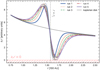 |
Fig. 1 Initial gradient in specific angular momentum ℓ
for our 5 simulations (thick lines, ranked from coldest to hottest) compared to the Keplerian case. The width of the density “jump” region σj
is adjusted in two steps. First, the critical value |


2.2 Boundary conditions
Boundary conditions are imposed through ghost cells outside of the domain and wave-killing region in the active domain. In the radial direction, ghost cells are fixed to the initial equilibrium values for density and azimuthal momentum. The radial momentum is copied from the first cells to the ghost cells at the inner boundary, and extrapolated linearly with no-inflow condition atthe outer edge. However, these boundary conditions have low impact as standard damping zones (de Val-Borro et al. 2006) are also used to avoid reflections at domain edges. The domain is periodic in the azimuthal direction.
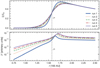 |
Fig. 2 Initialradial profiles in surface density (top) and the |


2.3 Rossby wave instability and vortex formation
Rossby wave instability is similar to the Kelvin-Helmholtz instability in a differentially rotating Keplerian disk. The instability tends to convert excess shear into vorticity. Lovelace et al. (1999) showed that a local extremum in the background potential vorticity is a necessary condition to RWI. More recent works have clarified that a minimum is required (Lai & Tsang 2009; Ono et al. 2016). The key function is defined as
 (5)
(5)
We exhibit this key function within our initial setup in Fig. 2, showing the existence of a local maximum in  , corresponding to a minimum in vorticity.
We find that, in order to excite the RWI unstable modes, it is useful to add random perturbations. We chose to perturb the radial velocity, which is zero otherwise, as
 (6)
(6)
where ψ(r, φ) ∈ [−10−2, 10−2] is a uniformly distributed random variable drawn for each grid cell. After the instability has saturated, we obtain a single vortex shown in Fig. 3. In a frame that is co-rotating with the vortex, its global structure is quasi-stationary as shown in Fig. 4. The radial density profile at the azimuth of the density maximum is plotted at different times. The orange dotted curve at t = 10 features the most noticeable fluctuations, as smaller eddies are still undergoing a merger and strong spiral waves are launched outward. After 40 orbital periods, the surface density of the vortex is stabilized and does not rapidly evolve any more. Thus we consider this state as quasi-stationary; we take a look at the dynamics of the structure in the next section.
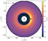 |
Fig. 3 Gas surface density plotted in Cartesian coordinates (x, y) after t = 200 orbital periods (t*). The globaldensity maximum is indicated by a black cross. The position of the central star is denoted as a “⋆” symbol. Thesimulation box radial limits are drawn as solid black circles, while the dashed-line circles indicate the limits of wave damping zones. |
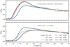 |
Fig. 4 Time evolution of the radial density profile, plotted as slices at the azimuth of the density maximum where the vortex eye lies (top) and its radial opposite (bottom). The slices correspond to the y = 0 axis in Fig. 3, with x > 0 (top) and x < 0 (bottom), respectively. After ~40 orbital periods, the disk has practically reached a stationary state. The cavity profile itself has become uneven, showing a non-zero eccentricity. |
3 Vortex signatures in dynamics
In this section, we provide observational signatures obtained from the dynamics of the vortex. The observable studied in this work is the velocity projected along the line of sight vLOS. We first discuss an adequate decomposition of the velocity field to characterize the signatures. We then study their observability against disk orientation and provide insight into how disk aspect ratio affects observed velocities.
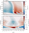 |
Fig. 5 Polar components of a the velocity field of a vortex. Top: radial velocity. Bottom: azimuthal velocity, where the axisymmetric part ⟨vφ⟩ is carried out. The pressure maximum is indicated by a black cross. The snapshot is taken at t = 200 orbital periods. The dotted line in the bottom panel indicates fluid in exact Keplerian rotation. |
3.1 Extracting dynamical signatures
The dynamics of a disk is dominated by rotation around the central star. In an axisymmetric stationary state, the net radial force is zero, as in Eq. (4). Owing to pressure gradients, the radial equilibrium slightly departs from Keplerian motion. This is the sub-Keplerian rotation in a disk with negative radial pressure gradient. As a dynamical structure, a vortex exposes little difference to global rotation. Thus, it is useful to decompose the angular velocity vφ as
 (7)
(7)
where ⟨⋅⟩ is the azimuthal average operator, and we denote the non-axisymmetric part as  . Hence the total velocity field v can be decomposed in the polar basis (er, eφ) as
 (8)
(8)
In the absence of a global accretion flow, there is no relevant axisymmetric part in vr. Hence we consider that dynamical signatures of non-axisymmetric features reside in 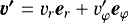 . Both components of this residual radial and azimuthal velocity are quantified in Fig. 5 and are of similar amplitudes. For comparison, the typical Keplerian speed at the vortex position (r ~ 180 AU) is vK = 3.3 km s−1, that is, one to two orders of magnitudes larger than the deviation due to the vortex, and one order of magnitude larger than the local sound-speed cs. The amplitude in the azimuthal velocity is as high as 300 m s−1 for this reference (coldest) model. This sets a first upper limit to the spectral resolution required for a direct detection to about 100 m s−1. This is achievable for bright lines with the Atacama Large Millimeter/submillimeter Array (ALMA), for example, for the CO (2-1) or the CO (3-2) transitions, using channel widths of 70 or 120 kHz (or narrower), respectively. For example, van der Marel et al. (2016) successfully detected the 13CO (3-2) and C18O (3-2) lines of SR21, HD 135344B, DoAr44, and IRS 48 with good signal-to-noise ratio (S/N) (peak S/N in the integrated intensity map up to 30 for the 13CO line) with spectral resolution of0.1 km s−1 and angular resolution of 0.′′25. Boehler et al. (2017) obtained data with similar angular and spectral resolutions for HD 142527 but with much higher S/N. All sources are well detected in the lines; increasing the spectral resolution by another factor of 2, as well as the S/N, is possible within a reasonable amount of time (<12 h). We note that there is a non-zero azimuthal velocity deviation at the maximum density/pressure (i.e.
  ), as seen in Fig. 5. Because the vortex is an asymmetric structure, the radial position of the pressure extremum varies with the azimuth. Consequently, the line of exact Keplerian rotation is not circular as shown in Fig. 5.
However, the decomposition proposed in Eq. (8) is vain unless the proposed dominant term ⟨vφ ⟩ can be subtracted from observations. While a Keplerian fit is usually a suiting approximation of the dominant velocity term, it proves insufficient near sharp density jumps. As shown in Figs. 6a and b, subtracting a Keplerian power law leaves systematic velocities caused by pressure gradients. In the density transition region, those systematics dominate over the variability in the remaining signal.
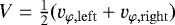
However, we further show (Figs. 6b and c) that averaging two facing cross sections in azimuthal velocities consistently yields a much better approximation for the global azimuthal average ⟨vφ ⟩, with a standard deviation ≤20 m s−1. This is a direct sign that the non-axisymmetric parts of the azimuthal velocities  in opposing disk halves are anticorrelated, although not strictly equal in amplitudes. Given that detection is only sensitive to azimuthal velocities on the observational major axis x of the disk, we naturally obtain a satisfying method to subtract ⟨vφ⟩ from the whole signal. Consequently, we now confidently assume that the axisymmetric part ⟨vφ ⟩ of the azimuthal velocity can indeed be removed with good precision from observations, and we only consider the remaining components of v′ exhibited in Fig. 5.
 |
Fig. 6 Comparison between Keplerian velocity vK and average azimuthal velocity ⟨vφ⟩ as 1D masks.(a) Pressure profile in arbitrary units. (b and c) Azimuthal velocity cross-sections, with offsets (masks) vK and ⟨vφ ⟩, respectively. The average ⟨V −mask⟩ is indicated by a thick black line, while shadows show the amplitude and standard deviations in blue (V = vφ), and orange ( |
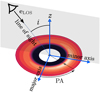 |
Fig. 7 Sketch view of our notations. The gray shadow shows the plane containing the vertical ez and the line of sight. |
3.2 Vortex detection in line-of-sight velocities
Gas velocity is usually detected through Doppler-shifting in molecular lines. It is therefore the velocity component parallel to the line of sight that is probed. Within optically thick lines, the resulting velocity profile can be blurred by vertical integration over disk height. It is beyond the scope of the present work to investigate this second-order effect, so we neglect both optical and geometrical thickness effects. This approach is reasonable within the assumption that emissive molecular regions are geometrically thin and well resolved (as remarked by Teague et al. 2018b). Furthermore, full 3D simulations showed that, in a stationary state, a vortex tends to be tubular and that its vertical velocity is negligible (Lin 2012; Zhu & Stone 2014; Richard et al. 2013). This comforts us in the idea that, for long-lived vortices, it is reasonable to ignore this component. This also means we ignore the vertical extension in the conical shape of the emissive layer. However, it can easily be shown that for inclinations lowers than 45°, even a very high emissive layer z ≃ 5H and a large aspect ratio H∕r = 0.2, can in principle be deprojected as long as it remains spatially thin.
To study vortex dynamical signatures, we use here cylindrical coordinates centered on the star. The radial axis (φ = 0) is the observational major axis, and the upper part of the disk (z > 0) is defined tobe the one seen by the observer Fig. 7.
Thus, the line-of-sight direction eLOS(i, φ), defined as pointing away from the observer, can be written in the disk cylindrical basis (er, eφ, ez) as
 (9)
(9)
and it follows that the line-of-sight velocity corresponding to v′ is written as
 (10)
(10)
Hence, the effective observable  mixes vr and vφ. For a 2D vortex disk inclination equally affects all projected velocities and only acts as a scaling factor sin (i). An inclination i = 27°, corresponding to the estimated value for HD 142527 (Fukagawa et al. 2013), is used in the following applications. This choice is arbitrary and used as a textbook case. We note that this inclination is moderate. Deprojection would still be feasible at up to i = 45°, where projected velocities would be 1.5 times larger, making detection easier. Figure 8 shows the morphology of the observable
  (large panels), along with corresponding components vr and
  (small panels), for four different values of PA. This result constitutes an idealized case, built on the assumption that the axisymmetric component ⟨vφ ⟩ can be exactly subtracted from observational data. We note that we are set in the particular case where the PA rotates in the same direction as the disk. When not so, sign in
  must simply be inverted. At all position angles (PAs), the anticyclonic motion of the vortex around the density maximum is apparent in
  . This point roughly coincides with the maximum luminosity at most wavelengths, and can be located within continuum observations, if not directly in molecular lines used to infer projected velocities.
We note that the eye of the vortex and the region immediately facing it have similar Doppler shifts (e.g., both blue at PA = 0°). This is an expected outcome of subtracting the azimuthally averaged velocity, since the both regions are local extrema along the azimuthal direction. Another signature of the vortex is the azimuthal proximity between the maximum density (black cross) and the projected velocity extrema. The latter two points are determined by the physical on-site velocity as well as the inclination of the system, and hence are virtual positions. Their physical separation is maximized for PA = 90° and minimized for PA = 0°. A direct implication is that detecting a vortex lying on the major axis requires greater angular resolution. However, little dependence of the velocity range on the PA is found. The topography of the signal changes with the PA but the anticyclonic region stands out regardless the orientation. The signature is also typical with a sign reversal in the vicinity of the pressure maximum, along the major axis direction. This characteristic behavior, sign change, is easier to measure in relative than the absolute small velocities and would be observed even with a beam covering the vortex almost entirely (about 100 AU, or 0.′′ 6 in the case of HD 142527).
3.3 Detectability against disk temperature
Although our setup is constrained by observations, its temperature (or equivalently h) is not. Indeed the temperature gives the sound speed, which is fundamental to estimate the vortex velocity. To study this dependence, four additional simulations with higher temperatures (h ∈ [0.094, 0.119, 0.136, 0.150, 0.161]) were performed. In Fig. 9, we show contours of projected velocity  , sampled at an interval corresponding to a tenth of the obtained dynamical range, namely 10 m s−1. The reference, “coldest” setup produces the lowest velocities ranging from −20 to +20 m s−1, where most of the “detected” structure is within the vortex region. The direct observation of a peak-to-valley velocity shift of about 40 m s−1 is challenging but is within reach of ALMA. Boehler et al. (2017) observed HD 142527 for a total of four hours during Cycle 1, targeting the continuum and 13CO (3–2) and C18 O (3–2) lines with a spectral resolution of 110 m s−1 (after Hanning smoothing). The disk is detected in both lines at high S/N. The angular resolution of the observations was 45 AU (beam 0.′′27 × 0.′′ 31). The presence of a velocity signature is currently being investigated in that data set (Boehler et al., in prep.). This angular resolution is sufficient to resolve the vortex in HD 142527 and the spectral resolution can be improved by a factor of 2 on the brighter 12CO line (Perez et al. 2015), or on the 13CO and C18O lines by increasing the time spent on-source.
At higher temperatures, more structure is revealed as the spiral arm unravels. Figure 10 shows the  variation amplitude, against temperature (left panel) and time (right panel). Although the upper bound of this range consistently increases with temperature, we note that the mean value is almost unchanged from run 4 to run 5. Indeed, in runs 3 to 5, the amplitude of time variations are significantly higher than for the reference run. These large variations are related to the life cycle of a secondary spiral arm that appears in hot cases, as illustrated in Fig. 11. However, because this secondary spiral is most prominent when the disk itself becomes visibly eccentric, it is likely that this structure would be affected if the indirect gravitational terms were included in the model. A conservative conclusion is that only the lower boundary of the variation interval should be taken into account. Additionally, we observe that between runs 4 and 5, the dynamical range stagnates at 94 m s−1. Indeed, this is the range shown in Fig. 9, where the simulations are shown at a time (t∕t* = 200) that minimizes its amplitude. This saturation is likely caused by the instability in the eccentricity of the cavity, thus we infer that validity of massless disk models is disputable in the hottest case (run 5). We note that a previous study of the gas dynamics in HD 142527 (Casassus et al. 2015b) did not provide evidence of any strong asymmetric structure. This may indeed be due to a lack of spectral resolution (~ 1 km s−1).
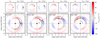 |
Fig. 8 Line-of-sight velocities (bottom large panels) as defined in Eq. (10), applied to HD 142527 with i = 27 °, and varying PA. Top panels: exhibit the corresponding polar components. Color reflects implied Doppler-shifts in molecular lines. Blue/orange dots indicate extreme values in
|

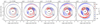 |
Fig. 9 Comparative view of |

3.4 RWI spirals
Spirals structures are detected in HD 142527 (Fukagawa et al. 2006; Casassus et al. 2012; Rameau et al. 2012; Avenhaus et al. 2014; Christiaens et al. 2014). Several scenarios have been proposed to understand their origin, such as self-gravitational instability (SGI), excitation by the stellar companion (Biller et al. 2012; Astropy Collaboration 2018), connection to a shadow cast by a misaligned inner disk (Montesinos et al. 2016), or a combination of several effects (Christiaens et al. 2014). Spirals are also a natural outcome of RWI, as Rossby waves are coupled to spiral density waves in a Keplerian disk. Such spiral waves would have the same frequency as the Rossby wave creating the vortex.
As opposed to companion-excited spirals, those are not caused by gravitational interaction and are observed in massless disks simulations such as ours (Huang et al. 2019). For Rossby vortices, the launching point is radially close to the vorticity extremum and the spiral corotates with the vortex. As a consequence, for spiral arms with different launching points, the RWI explanation may be safely rejected.
However, it must be noted that the apparent launching point of the spiral, that is, the origin of its detectable part, graphically indicated as a blue hatched mark, departs from its physical origin, namely the eye of the vortex. For instance, Fig. 9 shows a ~90° discrepancy between the actual launching point and the apparent origin of the main spiral arm. The figure also shows that, considering only spectral resolution as an experimental limitation, plane-RWI spirals are detectable as soon as the sensitivityis sufficient to resolve the bulk signature of the vortex. In short, spirals produce projected velocities just marginally smaller than the vortex’s bulk. We further note that plane-RWI spirals are a pure tracer of radial velocities vr, which are observationally characterized by a change of sign in projected velocities across the major axis.
We note that the pitch angle of the spiral increases with h, as a consequenceof a higher sound speed. Hence, radial velocities are not self-similar across our models, as hotter disks produce higher Mach numbers, as illustrated in Fig. 12.
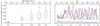 |
Fig. 10 Amplitude in |

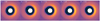 |
Fig. 11 Formation/dissipation cycle of a secondary spiral arm connected with disk eccentricity, illustrated for the most prominent case, run 5. Color maps density (same scale as Fig. 3). This secondary spiral is a transient and periodic phenomenon, which is responsible for large oscillations in maximum projected velocity as measured in Fig. 10 |
 |
Fig. 12 Radial Mach number vs. temperature (h), seen in polarcoordinates. The color maping is such that sub-(super)sonic regions appear in blue (red). The vortex center is always located at φ = 0. The dashed black lines indicate vφ = vK. The global structure is not self-similar when h varies, as one can see the Keplerian line undergoes a reconnection as temperature increases, and spirals in the outer disk are shocking(Mach 1, white) closer to the vortex. Small supersonic (red) regions are found in the inner region of the disk (r ≃ 120 AU), as is highlighted in an inset in the rightmost panel. The flow remains subsonic everywhere else. |
4 Discussion
4.1 Numerical versus practical differences
In Sect. 3.1, we showed that a promising data reduction strategy for vortex dynamic extraction in sharp density jumps was to subtract ⟨vφ ⟩, and that the projected velocity seen on the major axis ( for shorts) gives a reasonable proxy for it. In order to test the error implied by this approximation, this strategy is applied in Fig. 13. Consistently with our previous estimation, this more realistic view shows very little difference to the first, idealized estimation (Fig. 8). Figure 14 quantifies that 2D discrepancy as a difference between the numerical and practical cases. We find the discrepancy to reach at most ~ 7 m s−1.
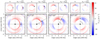 |
Fig. 13 Practical application of our data reduction method. The figure is similar to Fig. 8 except that
|

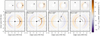 |
Fig. 14 Difference between numerical (Fig. 8) and practical (Fig. 13) cases. By construction,
|

4.2 Spiral detection
As shown inSect. 3.4, the projected velocities seen in spiral arms are comparable in amplitude to those attained by the core of the vortex core. However, angular resolution might constitute an additional limitation to identify those secondary structures. In Fig. 15 we simulate a limited angular resolution via Gaussian kernel convolution to the simulated velocity map, where the mean component of azimuthal velocity ⟨vφ ⟩ is subtracted prior to projection. We observe that the contrast sharpness of the main spiral pattern is altered but not destroyed by limited spatial resolution alone. We note that the spiral arm appears marginally broader in Fig. 13 as compared with the numerical case Fig. 8. The velocity flip pattern however remains visible and is unaltered by the limited spatial resolution.
4.3 Origin of the cavity in HD 142527
The most up-to-date simulations for the thermal emission of HD 142527 were performed in smooth-particle hydro (SPH) by Astropy Collaboration (2018) and do not feature vortex formation. This study was focused on explaining as many features as possible with the excitation provided by the eccentric stellar companion. However, it must be noted than SPH solvers generate numerical viscosities ~ 10−2 (Arena & Gonzalez 2013), which are much greater than typical values used in RWI vortex studies3 (Lyra et al. 2009; Hammer et al. 2017, 2019; Ono et al. 2016), so this possibility was inherently not included in their study. In the present work, we remained agnostic regarding how the initial unstable density jump was formed. The stellar companion, while not includedin our model, provides a plausible cause to the cavity. However, gravitational perturber-induced Rossby vortices have been studied in the context of circular orbital motion (Li et al. 2005). How eccentricity and inclination in the orbit of the companion affects the formation of vortices, within an appropriately inviscid medium, remains to be studied.
 |
Fig. 15 Qualitative comparison between a simulation-precision velocity map (left), and against artificially lowered spatial resolution, simulation with a Gaussian kernel convolution. Kernels with angular size (in proportions of the target) 7% (center), and a 3 times larger one 21% (right) are shown. With the distance of HD 142527, the center panel corresponds to the recent high resolution obtained by Keppler et al. (2019). No noise is added. Projected velocities are shown in linear gray-scale, where
|


4.4 Limits of this approach
An important limitation of the model is the lack of a vertical dimension. In a more realistic context, plane velocities (vr, vφ) are only detectable if the disk is inclined, which in turn affects measurements by line-of-sight integration. This effect would however be mitigated by choosing optically thick molecular lines. Moreover, Méheut et al. (2012b) showed that 3D vortices have a non-negligible vertical velocity component while they form (typically 10% of the characteristic azimuthal velocity signature). As the RWI growth time is typically shorter than the vortex lifetime by one or two orders of magnitude, it seems reasonable to neglect vertical circulation.
It has been shown that the contribution of the disk to the gravitational potential, promotes disk eccentricity (Regály & Vorobyov 2017b), which in turn amplifies the proper velocity of the vortex. Because this effect is neglected in our model, we expect the resulting velocities to be slightly underestimated in this work.
5 Conclusions
We showed that in cavity-hosting circumstellar disks, large eddies produce dynamical signatures on the verge of detectability for current facilities.
As the dynamical imprint of a vortex resides in the non-axisymmetric part of the velocity field, it is crucial to the detection to be able to subtract the axisymmetric component from observations. In the case of a vortex formed at the inner edge of a cavity-hosting disk, a Keplerian power law is not a correct proxy for the mean azimuthal velocity. This is because pressure gradients prone to vortex formation imply large deviations from Keplerian velocities. Nevertheless, as projected velocities of the observational major axis directly map the azimuthal motion, a better mask can be obtained by averaging both sides of the velocity profile on this axis. This approach proved to produce small errors when compared with the actual azimuthal mean component of velocity ⟨vφ ⟩. We also observed a saturation in the amplitude of projected velocities as the temperature is increased. This result is to be taken with a grain of salt and may point to a limitation of the model we used. Using this amplitude as an estimator for spectral resolution requirement, we conclude that detection of a single large eddy is achievable under a 50–150 m s−1 resolution, while the current maximal resolution with ALMA is ~ 30 m s−1 We stress that those minimal requirements were obtained within the particular case of the HD 142527 target, with a relatively low inclination (27°). Minimal resolution would be amplified by a factor 150% for a more likely, mean inclination of 45°, ceteris paribus. This demanding requirement may explain the current difficulty elucidate in elucidating the nature of known dust clumps in cavity-hosting disks, yet this is achievable with existing facilities. Vortex-free mechanisms could also explain their formation, although observational constraints for fine gas dynamics are needed to properly discriminate between concurrent scenarios. Full 3D modeling would naturally extend the present work, and allow the study of second order effects in line-of-sight integration.
Acknowledgements
C.M.T.R.’s Ph.D. grant is part of ANR number ANR-16-CE31-0013 (Planet-Forming-Disks). Computations were performed with OCCIGEN CINES (allocation DARI A0060402231), and “Mésocentre SIGAMM”, hosted by Observatoire de la Côte d’Azur. The data presented in this work were proceeded and plotted with Python’s data science ecosystem scipy, numpy (van der Walt et al. 2011), matplotlib (Hunter 2007), pandas (McKinney 2010) as well as astropy (Astropy Collaboration 2013, 2018) and the yt framework (Turk et al. 2011). C.M.T. is thankful to Aurélien Crida and Elena Lega for their early proofreading. The authors wish to thank the referee, Zsolt Regàly, for helping in improving the quality of the paper.
Appendix A Evaluations of aspect ratios
A.1 Equivalence to locally isothermal
Our model differs from the widely used locally isothermal prescription in that it is not defined in terms of scale height
 (A.1)
(A.1)
where h is the disk aspect ratio and β is the flaring. We can nonetheless draw an equivalence with those parameters for the power-law density distribution at the core of Eq. (3), such that  . In the locally isothermal prescription, the scale height is usually defined such that
  , so we can equate this with Eq. (A.1) to get
 (A.2)
(A.2)
at which point we deduce an effective aspect ratio and disk flaring, in terms of the actual simulation parameters
![\begin{equation*}\left\{\!\!\begin{array}{l} h^2 = \frac{\gamma S \Sigma_0^{\gamma-1} r_*}{GM} ,\\[3pt] \beta = 1 - \gamma/2 = 1/6. \end{array}\right. \end{equation*}](/articles/aa/full_html/2020/09/aa37414-19/aa37414-19-eq29.png) (A.3)
(A.3)
We note that our fixed resolution corresponds to Δr∕H(rj) ≃ 0.04 for the reference model. Figure A.1 shows the resulting variation in h as we scale up Σ0, following Eq. (A.3).
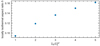 |
Fig. A.1 Correspondence between locally isothermal aspect ratio and “disk mass” in our simulations. The leftmost model is the reference. |
A.2 Spiral fitting
In Fig. 9, we fitted the linear-regime spiral wave shape (Goldreich & Tremaine 1979; Rafikov 2002; Muto et al. 2012) given by
![\begin{equation*} \begin{split}\hspace*{-4pt}&\varphi(r) = \varphi_o - \frac{\mathrm{sgn}(r-r_o)}{H_o} \\ &\times\left(\!(r/r_o)^{1+\beta} \left[\!\frac{1}{1+\beta}-\frac{1}{1-\alpha+\beta}(r/r_o)^{-\alpha}\!\right] - \left[\!\frac{1}{1+\beta}-\frac{1}{1-\alpha+\beta}\!\right]\right) , \end{split} \end{equation*}](/articles/aa/full_html/2020/09/aa37414-19/aa37414-19-eq30.png) (A.4)
(A.4)
where α, β are power-law exponents defined as Ω ∝ r−α and cs ∝ r−β, respectively. The quantities (ro, φo) are the coordinates of the spiral origin, while Ho is a scale height at this position. The fit was performed with Ho as a free parameter, so we the corresponding aspect ratio, differs from the locally isothermal equivalent h value used throughout the paper and described in the previous section. Figure A.2 shows values against each other.
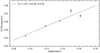 |
Fig. A.2 Aspect ratios as defined in Appendix A.1 vs. empirical values obtained from fitting Eq. (A.4). The latter is roughly 40% of the former. |
Appendix B Numerical viscosity evaluation
In order to estimate numerical viscosity νnum(r), performed a 1D in a 1D run, with identical parameterization as our reference 2D run (run1). The analytical initial conditions constitute a stable equilibrium since RWI cannot grow in 1D. Since our boundary conditions do not impose mass flux, any radial mass transport Ṁ through thesimulation domain is caused by numerical viscosity such that νnumΣ = |Ṁ|∕3π. In terms of the Shakura & Sunyaev (1973) alpha viscosity model νnum = αnumHcs, thus finally
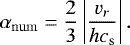 (B.1)
(B.1)
The obtained profile, time-averaged, is plotted in Fig. B.1. The highest numerical viscosities (αnum ~ 2 × 10⁻³) are reached in the cavity, while αnum stays bounded <10−4 in the vortex-forming region, roughly represented in orange.
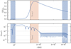 |
Fig. B.1 Density (top) and numerical viscosity equivalent α value (bottom) time-averaged over 10 orbital periods (t∕t*∈ [90, 100]) with a sampling rate of 0.1 orbital periods. The solid blue shadows indicate the variation interval over the sample time series, showing that the profile is very stable in the region of interest. The hatched regions highlight the wave-killing zones, while the orange region loosely indicates the vortex-forming region, spanning one scale height away from the local density maximum. |
References
- Adams, F. C., & Watkins, R. 1995, ApJ, 451, 314 [NASA ADS] [CrossRef] [Google Scholar]
- Andrews, S. M., Terrell, M., Tripathi, A., et al. 2018, ApJ, 865, 157 [NASA ADS] [CrossRef] [Google Scholar]
- Arena, S. E., & Gonzalez, J.-F. 2013, MNRAS, 433, 98 [CrossRef] [Google Scholar]
- Astropy Collaboration (Robitaille, T. P., et al.) 2013, A&A, 558, A33 [NASA ADS] [CrossRef] [EDP Sciences] [Google Scholar]
- Astropy Collaboration (Price-Whelan, A. M., et al.) 2018, AJ, 156, 123 [Google Scholar]
- Ataiee, S., Pinilla, P., Zsom, A., et al. 2013, A&A, 553, L3 [NASA ADS] [CrossRef] [EDP Sciences] [Google Scholar]
- Ataiee, S., Dullemond, C. P., Kley, W., Regály, Z., & Meheut, H. 2014, A&A, 572, A61 [NASA ADS] [CrossRef] [EDP Sciences] [Google Scholar]
- Avenhaus, H., Quanz, S. P., Schmid, H. M., et al. 2014, ApJ, 781, 87 [NASA ADS] [CrossRef] [Google Scholar]
- Barge, P., & Sommeria, J. 1995, A&A, 295, L1 [NASA ADS] [Google Scholar]
- Baruteau, C., Barraza, M., Pérez, S., et al. 2019, MNRAS, 486, 304 [CrossRef] [Google Scholar]
- Benisty, M., Juhasz, A., Facchini, S., et al. 2018, A&A, 619, A171 [NASA ADS] [CrossRef] [EDP Sciences] [Google Scholar]
- Biller, B., Lacour, S., Juhasz, A., et al. 2012, ApJ, 753, L38 [NASA ADS] [CrossRef] [Google Scholar]
- Birnstiel, T., Dullemond, C. P., & Pinilla, P. 2013, A&A, 550, L8 [NASA ADS] [CrossRef] [EDP Sciences] [Google Scholar]
- Boehler, Y., Weaver, E., Isella, A., et al. 2017, ApJ, 840, 60 [NASA ADS] [CrossRef] [Google Scholar]
- Bracco, A., Chavanis, P. H., Provenzale, A., & Spiegel, E. A. 1999, Phys. Fluids, 11, 2280 [NASA ADS] [CrossRef] [Google Scholar]
- Casassus, S., & Pérez, S. 2019, ApJ, 883, L41 [CrossRef] [Google Scholar]
- Casassus, S., Perez M., S., Jordán, A., et al. 2012, ApJ, 754, L31 [NASA ADS] [CrossRef] [Google Scholar]
- Casassus, S., Wright, C., Marino, S., et al. 2015a, ApJ, 812, 126 [NASA ADS] [CrossRef] [Google Scholar]
- Casassus, S., Marino, S., Pérez, S., et al. 2015b, ApJ, 811, 92 [NASA ADS] [CrossRef] [Google Scholar]
- Cazzoletti, P., van Dishoeck, E. F., Pinilla, P., et al. 2018, A&A, 619, A161 [NASA ADS] [CrossRef] [EDP Sciences] [Google Scholar]
- Casassus, S., Marino, S., Lyra, W., et al. 2019, MNRAS, 483, 3278 [CrossRef] [Google Scholar]
- Chiang, E., & Youdin, A. 2010, Ann. Rev. Earth Planet. Sci., 38, 493 [Google Scholar]
- Christiaens, V., Casassus, S., Perez, S., van der Plas, G., & Ménard, F. 2014, ApJ, 785, L12 [Google Scholar]
- de Val-Borro, M., Edgar, R. G., Artymowicz, P., et al. 2006, MNRAS, 370, 529 [NASA ADS] [CrossRef] [Google Scholar]
- de Val-Borro, M., Artymowicz, P., D’Angelo, G., & Peplinski, A. 2007, A&A, 471, 1043 [NASA ADS] [CrossRef] [EDP Sciences] [Google Scholar]
- Dong, R., Liu,S.-Y., Eisner, J., et al. 2018, ApJ, 860, 124 [NASA ADS] [CrossRef] [Google Scholar]
- Fu, W., Li, H., Lubow, S., & Li, S. 2014, ApJ, 788, L41 [NASA ADS] [CrossRef] [Google Scholar]
- Fukagawa, M., Tamura, M., Itoh, Y., et al. 2006, ApJ, 636, L153 [NASA ADS] [CrossRef] [Google Scholar]
- Fukagawa, M., Tsukagoshi, T., Momose, M., et al. 2013, Publ Astron Soc Jpn Nihon Tenmon Gakkai, 65 [Google Scholar]
- Gaia Collaboration (Brown, A. G. A., et al.) 2016, A&A, A595 [Google Scholar]
- Goldreich, P., & Tremaine, S. 1979, ApJ, 233, 857 [Google Scholar]
- Hammer, M., Kratter, K. M., & Lin, M.-K. 2017, MNRAS, 466, 3533 [CrossRef] [Google Scholar]
- Hammer, M., Pinilla, P., Kratter, K. M., & Lin, M.-K. 2019, MNRAS, 482, 3609 [NASA ADS] [CrossRef] [Google Scholar]
- Harten, A., Lax, P. D., & van Leer, B. 1983, SIAM Rev., 25, 35 [Google Scholar]
- Huang, P., Dong, R., Li, H., Li, S., & Ji, J. 2019, ApJ, 883, L39 [CrossRef] [Google Scholar]
- Hunter, J. D. 2007, Comput. Sci. Eng., 9, 99 [Google Scholar]
- Isella, A., Huang, J., Andrews, S. M., et al. 2018, ApJ, 869, L49 [NASA ADS] [CrossRef] [Google Scholar]
- Kataoka, A., Tsukagoshi, T., Momose, M., et al. 2016, ApJ, 831, L12 [NASA ADS] [CrossRef] [Google Scholar]
- Keppler, M., Teague, R., Bae, J., et al. 2019, A&A, 625, A118 [NASA ADS] [CrossRef] [EDP Sciences] [Google Scholar]
- Koren, B. 1993, Numerical Methods for Advection-Diffusion Problems (Braunschwelg, Wlesbaden: Vieweg), 117 [Google Scholar]
- Lai, D., & Tsang, D. 2009, MNRAS, 393, 979 [NASA ADS] [CrossRef] [Google Scholar]
- Li, H., Finn, J. M., Lovelace, R. V. E., & Colgate, S. A. 2000, ApJ, 533, 1023 [NASA ADS] [CrossRef] [Google Scholar]
- Li, H., Colgate, S. A., Wendroff, B., & Liska, R. 2001, ApJ, 551, 874 [NASA ADS] [CrossRef] [Google Scholar]
- Li, H., Li, S., Koller, J., et al. 2005, ApJ, 624, 1003 [NASA ADS] [CrossRef] [Google Scholar]
- Lin, M. 2012, AGU Fall Meeting Abstracts, 21, P2 1B [Google Scholar]
- Lovelace, R. V. E., Li, H., Colgate, S. A., & Nelson, A. F. 1999, ApJ, 513, 805 [NASA ADS] [CrossRef] [Google Scholar]
- Lyra, W., Johansen, A., Klahr, H., & Piskunov, N. 2009, A&A, 493, 1125 [NASA ADS] [CrossRef] [EDP Sciences] [Google Scholar]
- McKinney, W. 2010, in Proceedings of the 9th Python in Science Conference, 51 [Google Scholar]
- McNally, C. P., Nelson, R. P., & Paardekooper, S.-J. 2018, MNRAS, 477, 4596 [NASA ADS] [CrossRef] [Google Scholar]
- Méheut, H., Keppens, R., Casse, F., & Benz, W. 2012a, A&A, 542, A9 [Google Scholar]
- Méheut, H., Yu, C., & Lai, D. 2012b, MNRAS, 422, 2399 [NASA ADS] [CrossRef] [Google Scholar]
- Montesinos, M., Perez, S., Casassus, S., et al. 2016, ApJ, 823, L8 [NASA ADS] [CrossRef] [Google Scholar]
- Muto, T., Grady, C. A., Hashimoto, J., et al. 2012, ApJ, 748, L22 [NASA ADS] [CrossRef] [Google Scholar]
- Ono, T., Muto, T., Takeuchi, T., & Nomura, H. 2016, ApJ, 823, 84 [CrossRef] [Google Scholar]
- Perez, S., Casassus, S., Ménard, F., et al. 2015, ApJ, 798, 85 [Google Scholar]
- Pérez, S., Casassus, S., Hales, A., et al. 2020, ApJ, 889, L24 [CrossRef] [Google Scholar]
- Pineda, J. E., Szulágyi, J., Quanz, S. P., et al. 2019, ApJ, 871, 48 [Google Scholar]
- Pinte, C., Price, D. J., Ménard, F., et al. 2018, ApJ, 860, L13 [NASA ADS] [CrossRef] [Google Scholar]
- Pinte, C., van der Plas, G., Ménard, F., et al. 2019, Nat. Astron., 3, 1109 [Google Scholar]
- Porth, O., Xia, C., Hendrix, T., Moschou, S. P., & Keppens, R. 2014, ApJS, 214, 4 [Google Scholar]
- Price, D. J., Cuello, N., Pinte, C., et al. 2018, MNRAS, 477, 1270 [Google Scholar]
- Rafikov, R. R. 2002, ApJ, 572, 566 [NASA ADS] [CrossRef] [Google Scholar]
- Rameau, J., Chauvin, G., Lagrange, A.-M., et al. 2012, A&A, 546, A24 [NASA ADS] [CrossRef] [EDP Sciences] [Google Scholar]
- Rayleigh, J. W. 1879, Proc. Lond. Math. Soc., 1, 57 [CrossRef] [MathSciNet] [Google Scholar]
- Regály, Z., & Vorobyov, E. 2017a, MNRAS, 471, 2204 [NASA ADS] [CrossRef] [Google Scholar]
- Regály, Z., & Vorobyov, E. 2017b, A&A, 601, A24 [NASA ADS] [CrossRef] [EDP Sciences] [Google Scholar]
- Regály, Z., Juhasz, A., Sándor, Z., & Dullemond, C. P. 2012, MNRAS, 419, 1701 [NASA ADS] [CrossRef] [Google Scholar]
- Regály, Z., Sándor, Z., Csomós, P., & Ataiee, S. 2013, MNRAS, 433, 2626 [NASA ADS] [CrossRef] [Google Scholar]
- Richard, S., Barge, P., & Le Dizès, S. 2013, A&A, 559, A30 [NASA ADS] [CrossRef] [EDP Sciences] [Google Scholar]
- Shakura, N. I., & Sunyaev, R. A. 1973, A&A, 500, 33 [NASA ADS] [Google Scholar]
- Tanga, P., Babiano, A., & Dubrulle, B. 1996, Icarus, 121, 158 [NASA ADS] [CrossRef] [Google Scholar]
- Teague, R., & Foreman-Mackey, D. 2018, Res. Notes Am. Astron. Soc., 2, 173 [Google Scholar]
- Teague, R., Guilloteau, S., Semenov, D., et al. 2016, A&A, 592, A49 [NASA ADS] [CrossRef] [EDP Sciences] [Google Scholar]
- Teague, R., Bae, J., Bergin, E. A., Birnstiel, T., & Foreman-Mackey, D. 2018a, ApJ, 860, L12 [NASA ADS] [CrossRef] [Google Scholar]
- Teague, R., Bae, J., Birnstiel, T., & Bergin, E. A. 2018b, ApJ, 868, 113 [NASA ADS] [CrossRef] [Google Scholar]
- Turk, M. J., Smith, B. D., Oishi, J. S., et al. 2011, ApJS., 192, 9 [CrossRef] [Google Scholar]
- van der Marel, N., van Dishoeck, E. F., Bruderer, S., et al. 2016, A&A, 585, A58 [NASA ADS] [CrossRef] [EDP Sciences] [Google Scholar]
- van der Walt, S., Colbert, S. C., & Varoquaux, G. 2011, Comput. Sci. Eng., 13, 22 [Google Scholar]
- Verhoeff, A. P., Min, M., Pantin, E., et al. 2011, A&A, 528, A91 [NASA ADS] [CrossRef] [EDP Sciences] [Google Scholar]
- Xia, C., Teunissen, J., Mellah, I. E., Chané, E., & Keppens, R. 2018, ApJS, 234, 30 [Google Scholar]
- Yen, H.-W., Liu, H. B., Gu, P.-G., et al. 2016, ApJ, 820, L25 [NASA ADS] [CrossRef] [Google Scholar]
- Zhu, Z., & Baruteau, C. 2016, MNRAS, 458, 3918 [NASA ADS] [CrossRef] [Google Scholar]
- Zhu, Z., & Stone, J. M. 2014, ApJ, 795, 53 [NASA ADS] [CrossRef] [Google Scholar]
The model used in this paper is inviscid. Insights into our evaluation of numerical viscosity are given in Appendix B.
All Figures
|
Fig. 1 Initial gradient in specific angular momentum ℓ
for our 5 simulations (thick lines, ranked from coldest to hottest) compared to the Keplerian case. The width of the density “jump” region σj
is adjusted in two steps. First, the critical value |
| In the text | |
|
Fig. 2 Initialradial profiles in surface density (top) and the |
| In the text | |
|
Fig. 3 Gas surface density plotted in Cartesian coordinates (x, y) after t = 200 orbital periods (t*). The globaldensity maximum is indicated by a black cross. The position of the central star is denoted as a “⋆” symbol. Thesimulation box radial limits are drawn as solid black circles, while the dashed-line circles indicate the limits of wave damping zones. |
| In the text | |
|
Fig. 4 Time evolution of the radial density profile, plotted as slices at the azimuth of the density maximum where the vortex eye lies (top) and its radial opposite (bottom). The slices correspond to the y = 0 axis in Fig. 3, with x > 0 (top) and x < 0 (bottom), respectively. After ~40 orbital periods, the disk has practically reached a stationary state. The cavity profile itself has become uneven, showing a non-zero eccentricity. |
| In the text | |
|
Fig. 5 Polar components of a the velocity field of a vortex. Top: radial velocity. Bottom: azimuthal velocity, where the axisymmetric part ⟨vφ⟩ is carried out. The pressure maximum is indicated by a black cross. The snapshot is taken at t = 200 orbital periods. The dotted line in the bottom panel indicates fluid in exact Keplerian rotation. |
| In the text | |
|
Fig. 6 Comparison between Keplerian velocity vK and average azimuthal velocity ⟨vφ⟩ as 1D masks.(a) Pressure profile in arbitrary units. (b and c) Azimuthal velocity cross-sections, with offsets (masks) vK and ⟨vφ ⟩, respectively. The average ⟨V −mask⟩ is indicated by a thick black line, while shadows show the amplitude and standard deviations in blue (V = vφ), and orange ( |
| In the text | |
|
Fig. 7 Sketch view of our notations. The gray shadow shows the plane containing the vertical ez and the line of sight. |
| In the text | |
|
Fig. 8 Line-of-sight velocities (bottom large panels) as defined in Eq. (10), applied to HD 142527 with i = 27 °, and varying PA. Top panels: exhibit the corresponding polar components. Color reflects implied Doppler-shifts in molecular lines. Blue/orange dots indicate extreme values in
|
| In the text | |
|
Fig. 9 Comparative view of |
| In the text | |
|
Fig. 10 Amplitude in |
| In the text | |
|
Fig. 11 Formation/dissipation cycle of a secondary spiral arm connected with disk eccentricity, illustrated for the most prominent case, run 5. Color maps density (same scale as Fig. 3). This secondary spiral is a transient and periodic phenomenon, which is responsible for large oscillations in maximum projected velocity as measured in Fig. 10 |
| In the text | |
|
Fig. 12 Radial Mach number vs. temperature (h), seen in polarcoordinates. The color maping is such that sub-(super)sonic regions appear in blue (red). The vortex center is always located at φ = 0. The dashed black lines indicate vφ = vK. The global structure is not self-similar when h varies, as one can see the Keplerian line undergoes a reconnection as temperature increases, and spirals in the outer disk are shocking(Mach 1, white) closer to the vortex. Small supersonic (red) regions are found in the inner region of the disk (r ≃ 120 AU), as is highlighted in an inset in the rightmost panel. The flow remains subsonic everywhere else. |
| In the text | |
|
Fig. 13 Practical application of our data reduction method. The figure is similar to Fig. 8 except that
|
| In the text | |
|
Fig. 14 Difference between numerical (Fig. 8) and practical (Fig. 13) cases. By construction,
|
| In the text | |
|
Fig. 15 Qualitative comparison between a simulation-precision velocity map (left), and against artificially lowered spatial resolution, simulation with a Gaussian kernel convolution. Kernels with angular size (in proportions of the target) 7% (center), and a 3 times larger one 21% (right) are shown. With the distance of HD 142527, the center panel corresponds to the recent high resolution obtained by Keppler et al. (2019). No noise is added. Projected velocities are shown in linear gray-scale, where
|
| In the text | |
|
Fig. A.1 Correspondence between locally isothermal aspect ratio and “disk mass” in our simulations. The leftmost model is the reference. |
| In the text | |
|
Fig. A.2 Aspect ratios as defined in Appendix A.1 vs. empirical values obtained from fitting Eq. (A.4). The latter is roughly 40% of the former. |
| In the text | |
|
Fig. B.1 Density (top) and numerical viscosity equivalent α value (bottom) time-averaged over 10 orbital periods (t∕t*∈ [90, 100]) with a sampling rate of 0.1 orbital periods. The solid blue shadows indicate the variation interval over the sample time series, showing that the profile is very stable in the region of interest. The hatched regions highlight the wave-killing zones, while the orange region loosely indicates the vortex-forming region, spanning one scale height away from the local density maximum. |
| In the text | |
Current usage metrics show cumulative count of Article Views (full-text article views including HTML views, PDF and ePub downloads, according to the available data) and Abstracts Views on Vision4Press platform.
Data correspond to usage on the plateform after 2015. The current usage metrics is available 48-96 hours after online publication and is updated daily on week days.
Initial download of the metrics may take a while.