| Issue |
A&A
Volume 639, July 2020
|
|
|---|---|---|
| Article Number | A8 | |
| Number of page(s) | 8 | |
| Section | Stellar atmospheres | |
| DOI | https://doi.org/10.1051/0004-6361/202037953 | |
| Published online | 01 July 2020 | |
Understanding the rotational variability of K2 targets
HgMn star KIC 250152017 and blue horizontal branch star KIC 249660366★
1
Department of Theoretical Physics and Astrophysics, Masaryk University,
Kotlářská 2,
611,37
Brno,
Czech Republic
e-mail: krticka@physics.muni.cz
2
International Centre for Radio Astronomy Research, Curtin University,
GPO Box U1987,
Perth,
WA
6845, Australia
3
Space Research Institute, Austrian Academy of Sciences,
Schmiedlstrasse 6,
8042
Graz, Austria
4
Astronomical Institute, Academy of Science of CR,
Fričova 298,
251 65
Ondřejov,
Czech Republic
Received:
13
March
2020
Accepted:
14
May
2020
Context. Ultraprecise space photometry enables us to reveal light variability even in stars that were previously deemed constant. A large group of such stars show variations that may be rotationally modulated. This type of light variability is of special interest because it provides precise estimates of rotational rates.
Aims. We aim to understand the origin of the light variability of K2 targets that show signatures of rotational modulation.
Methods. We used phase-resolved medium-resolution X-shooter spectroscopy to understand the light variability of the stars KIC 250152017 and KIC 249660366, which are possibly rotationally modulated. We determined the atmospheric parameters at individual phases and tested the presence of the rotational modulation in the spectra.
Results. KIC 250152017 is a HgMn star, whose light variability is caused by the inhomogeneous surface distribution of manganese and iron. It is only the second HgMn star whose light variability is well understood. KIC 249660366 is a He-weak, high-velocity horizontal branch star with overabundances of silicon and argon. The light variability of this star is likely caused by a reflection effect in this post-common envelope binary.
Key words: stars: variables: general / stars: chemically peculiar / stars: horizontal-branch / stars: atmospheres / stars: early-type
© ESO 2020
1 Introduction
Rotationally modulated light variability is very common in intermediate-mass stars (e.g. Hümmerich et al. 2016; Sikora et al. 2019). This type of variability is typically connected with abundance spots in stars without deep subsurface convective layers (e.g. Krtička et al. 2015; Prvák et al. 2015), but may also have another origin, for example a magnetically confined circumstellar medium (Landstreet & Borra 1978; Townsend et al. 2005; Krtička 2016).
In main-sequence stars, abundance spots appear as a result of elemental diffusion, when the radiatively supported elements emerge on the surface in enhanced amounts, while the remaining elements sink down due to the effect of gravity (Michaud et al. 1983; Vauclair et al. 1991; Stift & Alecian 2012). Abundance spots are particularly pronounced in stars with strong magnetic fields, in which case Zeeman Doppler imaging techniques are frequently applied to constrain the spot structure (Piskunov & Kochukhov 2002; Kochukhov & Wade 2010).
The derived abundance maps can be used to simulate the light variability and to determine its origin. The variability of hotter main-sequence, chemically peculiar stars is typically dominated by the effects of bound-free transitions of helium and silicon (Peterson 1970; Krtička et al. 2007), while for cooler stars bound-bound transitions of heavy elements such as iron and chromium play a dominant role (Molnar 1973; Shulyak et al. 2010).
In contrast to stars with a strong magnetic field, according to the classical picture of non-magnetic, chemically peculiar stars of Am and HgMn types, these stars do not show any rotational variability, implying an absence of spots. This picture has been challenged by precise photometric and spectroscopic observations of these stars (Zverko et al. 1997; Adelman et al. 2002; Morel et al. 2014) showing surface spots that may even be evolving (Korhonen et al. 2013). However, evidence for photometric variability of these stars was not convincing until space photometry was used (Balona et al. 2011; Paunzen et al. 2013; Morel et al. 2014; Hümmerich et al. 2018), which provides brightness measurements with more than an order of magnitude better precision than ground-based photometry. Prvák et al. (2020) showed that surface abundance spots can explain the weak light variability of these stars.
Chemical abundance spots and peculiarities are typically found among main-sequence stars (Niemczura et al. 2015; Ghazaryan et al. 2019). However, the effects of radiative diffusion are not restricted to main-sequence stars, and they become especially strong in stars with high gravity, that is, hot subdwarfs and white dwarfs (Unglaub & Bues 2000, 2001; VandenBerg et al. 2002; Michaud et al. 2011). Subdwarfs typically lack strong magnetic fields (Landstreet et al. 2012) and the weakness of magnetic field confinement is possibly the reason for the absence of spots in blue horizontal branch stars (Paunzen et al. 2019).
On the other hand, white dwarfs show magnetic fields with diverse strengths (Valyavin et al. 2006; Kawka & Vennes 2011; Landstreet et al. 2016), but indications of surface abundance spots in white dwarfs are scarce (Dupuis et al. 2000; Reindl et al. 2019. Therefore, we took the list of white dwarfs observed by the Kepler satellite (Hermes et al. 2017), extracted those that most likely have significant rotational variability, and performed a detailed spectroscopic study to identify their nature. Here, we report the first results of this survey that led us to conclude that two previously considered white dwarfs possibly presenting rotational modulation are in reality less evolved stars: a HgMn star and a He-weak blue horizontal branch star.
Spectra used for analysis.
2 Observations and spectral analysis
We obtained spectra of KIC 250152017 and KIC 249660366 as part of the ESO proposal 0103.D-0194(A). The spectra were acquired with the X-shooter spectrograph (Vernet et al. 2011) mounted on the 8.2 m UT2 Kueyen telescope and these observations are summarized in Table 1. The spectra were obtained with the UVB and VIS arms providing an average spectral resolution (R = λ∕Δλ) of 9700 and 18 400, respectively. Although medium-resolution spectra are not ideal for abundance analysis, the abundance determination is based on multiple strong lines for most elements. This mitigates the disadvantages of the medium-resolution spectra and enables us to use even medium-resolution spectra for abundance analysis (e.g. Kawka & Vennes 2016; Gvaramadze et al. 2017). As a result, the difference due to the spectral resolution mostly affects the number of elements one can measure and with it the precision of those measured elements whose lines are blended by the elements that have not been measured. The calibrated spectra were extracted from the European Southern Observatory(ESO) archive. We determined the radial velocity from each spectrum by means of a cross-correlation function using the theoretical spectrum as a template (Zverko et al. 2007), and shifted the spectra to the rest frame.
We used simplex minimization to determine stellar parameters (Krtička & Štefl 1999). The analysis was performed in two steps. In the first step, we determined the effective temperature Teff and surface gravity log g by fitting the observed spectra with fixed abundances. In the second step, we fixed the effective temperature and surface gravity and determined individual abundances relative to hydrogen εel = log (nel∕nH) again by fitting the observed spectra. We analysed the normalized spectra, but to test the derived effective temperatures and surface gravities we additionally also fitted flux calibrated spectra. To this end and to account for possible systematics in the absolute flux calibration, we introduced a parameter that rigidly scaled the synthetic fluxes in the fitting procedure to the observed fluxes.
We processed each spectrum separately. For the analysis of KIC 250152017, we used ATLAS12 (Castelli 2005; Kurucz 2005) local thermodynamical equilibrium (LTE) model atmospheres. We applied the BSTAR2006 grid (Lanz & Hubeny 2007) and non-LTE (NLTE) TLUSTY models to determine the parameters of KIC 249660366. The spectrum synthesis was done using the SYNSPEC code (Lanz & Hubeny 2007), neglecting isotopic splitting.
Table 2 summarizes the available astrometric and photometric data for both stars. The coordinates and magnitudes were derived from the Mikulski Archive for Space Telescopes (MAST) K2 catalogue (Howell et al. 2014), while the parallax π and proper motions are taken from the Gaia data release 2 (DR2) data (Gaia Collaboration 2016, 2018). The distances d were determined from the parallax using the method described by Luri et al. (2018). The colour excesses were determined from Galactic reddening maps (Green et al. 2018) for locations corresponding to the stars. The space velocities in Table 2 were determined from Gaia DR2 proper motions and radial velocities using Johnson & Soderblom (1987).
Basic astrometric and photometric parameters of studied stars.
3 Chemically peculiar star KIC 250152017
The phases of KIC 250152017 spectra in Table 1 were determined with ephemeris (in barycenter corrected Julian date)
 (1)
(1)
derived from K2 photometry1 (see Mikulášek 2016, for details). Mean phase averaged parameters and their uncertainties derived from fitting the individual observed spectra by LTE models (see Fig. 1) are given in Table 3. The strongest lines used for the abundance determination are listed in Table 4.
Judging from the effective temperature Teff = 12160 ± 130 K and surface gravity log g = 3.95 ± 0.02, KIC 250152017 is a main-sequence star. An underabundance of He, C, Mg, and Si and an overabundance of Mn, Y, and Hg indicates that it belongs to the HgMn group of chemically peculiar stars (CP3, Preston 1974; Maitzen 1984; Ghazaryan et al. 2018). Mercury typically shows isotopic splitting in HgMn stars (White et al. 1976; Woolf & Lambert 1999; Aret & Sapar 2002) possibly affecting the derived abundance. We used the BONNSAI2 service (Schneider et al. 2014) to determine the evolutionary parameters of the star from observational parameters assuming solar metallicity evolutionary models (Brott et al. 2011). We derived a mass of M = 3.33 ± 0.08 M⊙, a radius of R = 3.19 ± 0.10 R⊙, and an age of 162 ± 10 Myr. With a known projection of rotational velocity of v sin i = 22 ± 5km s−1 and assuming that the period given in Eq. (1) is due to rotation, we determined the inclination as i = 42° ± 15°.
In addition, we determined the stellar parameters from flux calibrated data. The derived parameters Teff= 12 500 ± 100 K and log g = 3.92 ± 0.01 reasonably agree with values determined from normalized spectra.
The parameters derived from evolutionary tracks disagree with Gaia DR2 data. From a distance of 3200 ± 700 pc, the visual magnitude is mV= 14.726 ± 0.042 mag, the colour excess is E(B−V) = 0.12 ± 0.02, the bolometric correction is BC = −0.72 ± 0.03 mag (Flower 1996, see also Torres 2010), the deredened magnitude is V = 14.35 ± 0.07 mag, and the absolute bolometric magnitude is 1.1 ± 0.5 mag. This is significantly higher than the value derived from the evolutionary tracks, − 1.0 ± 0.1 mag. Using the effective temperature from spectroscopy, this implies a lower stellar radius of R = 1.2 ± 0.3 R⊙ than that derived from the evolutionary tracks. A lower radius gives a rotational velocity of vrot = 12±3 km s−1, which is significantly lower than the spectroscopically derived value. This most likely implies that the Gaia DR2 distance is incorrect, possibly due to the binary nature of the object.
The presence of a companion is common in HgMn stars (e.g. Ryabchikova 1998; Niemczura et al. 2017), but we have not detected radial velocity variations larger than about 10 km s−1 in KIC 250152017. Neither have we detected any features in the spectra that can be attributed to the companion. Therefore the maximum flux ratio of both components is about 0.1 in the VIS arm. This implies that the companion could be a main-sequence star of spectral type F5 or later (using main-sequence parameters from Harmanec 1988). Such a star would cause radial velocity variations below the detection limit even assuming tidal locking. Large V velocity (see Table 2) would imply that the object is either a member of the halo population or that it is a runaway star, however this is questionable given the problem with parallax.
Figure 2 shows that abundances of individual elements have phase-dependent variations. The phase variations of individual elements are mutually shifted. However, there seems to be a general trend that the heavier elements Si, Ti, Mn, and Fe vary in phase with the light curve, while Mg possibly varies in antiphase.
The periodic line profile variations in chemically peculiar stars are interpreted as a result of surface abundance spots (e.g. Lueftinger et al. 2003; Rusomarov et al. 2015), which also cause photometric variations (Krtička et al. 2007; Shulyak et al. 2010). Precise photometry of HgMn stars also reveals rotational variability (Morel et al. 2014; Strassmeier et al. 2017; Hümmerich et al. 2018). However, evidence of abundance spots on the surface of HgMn stars is scarce (Kochukhov et al. 2007; Briquet et al. 2010; Hubrig et al. 2010; Makaganiuk et al. 2011). The photometric variability in HgMn stars can be also attributed to flux redistribution due to modified opacity in abundance spots (Prvák et al. 2020).
To identify which elements may contribute to the light variability, in Fig. 3 we plot the relative magnitude difference Δm= −2.5log (Fel∕F*) between the flux Fel calculated with the abundance of a given element multiplied by a factor of 1.1, and the flux F* calculated for the chemical composition of KIC 250152017. The adopted multiplicative factor 1.1 corresponds to typical abundance variations found in Fig. 2. The fluxes used in Fig. 3 were smoothed by a Gaussian filter with a dispersion of 100 Å and evaluated atwavelength 6000 Å, which corresponds to the maximum of the Kepler response function. From Fig. 3 it follows that mostly manganese and iron contribute to the light variability of KIC 250152017.
We simulated light variations of KIC 250152017 assuming that one hemisphere has a greater abundance of Mn and Fe, higher than the other hemisphere by ΔεMn = 0.08 and ΔεFe = 0.05, respectively.These values correspond to the amplitudes of the abundance variations determined from the spectra in individual phases (Fig. 2, bottom panel). We calculated the synthetic spectra for individual abundances and integrated the specific intensities over the visible stellar surface and over the instrumental response curve (see Krtička et al. 2015, for more details of the code). We adopted a fit to the instrument response curve as derived from the Kepler Instrument Handbook (Van Cleve & Caldwell 2016) and given in the Appendix A. The predicted and observed light variations in Fig. 2 (upper panel) reasonably agree demonstrating that surface abundance variations of Mn and Fe are able to explain the observed light variability of KIC 250152017.
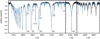 |
Fig. 1 Comparison of observed (black line) and best fit synthetic (blue line) spectra of KIC 250152017. |
Derived mean parameters of the studied stars compared to solar abundances (Asplund et al. 2009).
Wavelengths (in Å) of the strongest lines used for KIC 250152017 abundance determination.
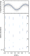 |
Fig. 2 Phase variations of KIC 250152017. Upper panel: K2 magnitudes. The solid line denotes a light curve simulated assuming surface abundance spots of manganese and iron corresponding to the observed spectral variations. Bottom panel: relative variations of abundances. Uncertainties were determined following Hosek et al. (2014). |
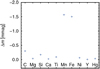 |
Fig. 3 Relative magnitude differences between flux at 6000 Å calculated with enhanced abundance of a given element and flux at KIC 250152017 abundances. |
4 He-poor high-velocity star KIC 249660366
The phases of KIC 249660366 spectra in Table 1 were determined using the ephemeris (in barycenter corrected Julian date)
 (2)
(2)
which was derived from K2 photometry (see Fig. 4). Mean (phase averaged) parameters of KIC 249660366 (Table 3) derived from fitting the individual spectra by NLTE models (Fig. 5) place the object below the solar metallicity main sequence (Fig. 6). The parameters derived from fitting flux calibrated spectra give a slightly higher effective temperature Teff = 20 600 ± 200 K and similar surface gravity log g = 4.64 ± 0.08 compared to the parameters derived from normalized spectra (Table 3). The star shows an underabundance of helium and light elements, and an overabundance of silicon and argon (see Table 5 for the list of analysed lines). With mV = 14.967 ± 0.045 mag and E(B−V) = 0.09 ± 0.02, the deredened V = 14.69 ± 0.08 mag. With the Gaia DR2 distance of 2200 ± 400 pc, the absolute magnitude is MV = 2.98 ± 0.40 mag, which with the bolometric correction BC = −1.86 ± 0.03 mag from Flower (1996, see also Torres 2010) and with spectroscopically determined parameters gives a stellar radius and mass of R = 0.45 ± 0.09 R⊙ and M = 0.27 ± 0.10 M⊙, respectively.These parameters are typical for subdwarfs and blue horizontal branch stars (Heber 2016).
The KIC 249660366 light curve (Fig. 4) could be explained either by binary effects, by pulsations, or by the abundance spots. If the light variations are due to ellipsoidal variability (distortion of the stellar surface), then the time of the observation should correspond to a period of relatively large changes in the radial velocity. The orbital period would be twice that determined in Eq. (2). Because there are no lines of the secondary star present in the spectra, we can assume that the total mass of the system is that of a putative primary. By using Kepler’s third law, we calculated the semi-major axis as 8.6 R⊙. We used our binary code that simulates the light curve assuming stellar distortion within the Roche model (adopting a companion mass of 0.2 M⊙) to predict the amplitude of the light variability. The derived amplitude is two orders of magnitude lower than the observed amplitude of the light variability. Subdwarfs are frequently found in binaries with degenerate components (Heber 2016). However, adopting a higher companion mass would imply larger binary separation and even lower amplitude of the light variability. Thus, we concludethat ellipsoidal variations due to a subdwarf component are unlikely to cause light variability in KIC 249660366.
The light variations in overcontact binaries may also produce light curves that have a nearly sinusoidal shape (Tylenda et al. 2011). In this case the true period would again be twice that determined in Eq. (2) and assuming an equal mass of each star of 0.3 M⊙ gives an orbital separation of 11 R⊙, which is significantly larger than the radius of a subdwarf. Consequently, the model of an overcontact binary also does not provide a reliable explanation of the KIC 249660366 light curve.
A large fraction of subdwarfs show light variations due to a reflection effect on a cool companion (Schaffenroth et al. 2019). Detailed modelling of such an effect is complex (e.g. Budaj 2011), so we just estimated the amplitude of expected light variations. Using R1, R2, T1, and T2 to denote the radii and effective temperatures of both components, the radiative power acquired by the companion from the Stefan-Boltzmann law  leads to an increase in the companion effective temperature of
 ![$T_2\left[{1+\left({T_1/T_2}^4\right) \left({R_1/(2a)^2}\right) }\right]^{1/4}$](/articles/aa/full_html/2020/07/aa37953-20/aa37953-20-eq4.png) . Using the Rayleigh-Jeans law, the amplitude of the magnitude change due to the reflection effect is then
. Using the Rayleigh-Jeans law, the amplitude of the magnitude change due to the reflection effect is then
![\begin{equation*}\Delta m\approx\frac{R_2^2T_2}{R_1^2T_1} \left\{{\left[{1+\left({T_1/T_2}^4\right) \left({R_1/(2a)^2}\right) }\right]^{1/4}-1 }\right\}. \end{equation*}](/articles/aa/full_html/2020/07/aa37953-20/aa37953-20-eq5.png) (3)
(3)
With orbital separation a derived from Kepler’s third law as a function of secondary mass, Eq. (3) gives the amplitude of the reflection effect as a function of the parameters of the secondary. We calculated the magnitude of the reflection effect using the main-sequence stellar parameters of Harmanec (1988) for a wide range of companions with T2 down to 3 kK. This analysis shows that a low-mass companion with M2 ≲ 0.5 M⊙ is able to cause the observed light variability due to the reflection effect and still its radiation will not affect the combined spectrum of the binary. The object shows only a marginal change in the radial velocities Δvrad = −3 ± 6km s−1 between the two spectra. This does not contradict the expected radial velocity curve in the case of a reflection effect, which should show maximum around phase 0.75, as follows from Fig. 4. We checked the presence of a putative companion using the spectral energy distribution constructed using the VOSA tool (Bayo et al. 2008). The observed flux limits the effective temperature of the main-sequence companion T2 ≤ 4 kK, which agrees with previous constraints. Consequently, the reflection effect provides plausible explanation of the KIC 249660366 light curve.
The light variations could also be caused by pulsations. The location of KIC 249660366 in the Hertzsprung-Russell diagram is close to the region populated by β Cep variables and by slowly pulsating B stars (Walczak et al. 2015). However, subdwarfs typically pulsate with periods of the order of a fraction of a day (Charpinet et al. 1996; Kilkenny et al. 1997; Østensen et al. 2010; Kawka et al. 2012), which is much shorter than the period found in KIC 249660366. Moreover, such stars typically show several pulsational periods, which is not the case for KIC 249660366. The studied star is slightly cooler than blue large-amplitude pulsators (Pietrukowicz et al. 2017). These are expected to be post-common-envelope objects on their way towards the white dwarf evolutionary stage, with pulsations driven by the opacity of iron-group elements (Byrne & Jeffery 2020). Also these objects pulsate with significantly shorter periods (of the order of tens of minutes) than found in KIC 249660366. Consequently, it is not likely that the light variations of KIC 249660366 originate from pulsations.
The remaining possibility is that the light variability is caused by surface spots, which are connected with peculiar abundances in hot stars (e.g. Lueftinger et al. 2003; Rusomarov et al. 2015). To search for a possible source of light variations, we calculated additional atmosphere models with an abundance of silicon and argon three times higher and ten times higher than the solar one, respectively. The enhancement of the abundance leads to an increase in the optical flux at 6000 Å by about 0.01 mag in the case of silicon and by 0.05 mag in the case of argon, which would explain the observed light variations.
We used the code of Prvák (2019) to test if the observed light variations can be reproduced by surface spots. The code uses procedure inspired by genetic algorithms to search for a surface brightness distribution that fits the observed light curve best. We assumed a maximum intensity contrast of 7%. The code fits the observed photometric variability using a large bright surface spot located at latitudes that nearly directly face the observer. The fit in Fig. 4 nicely reproduces the observed light curve.
If the light variations are caused by surface spots, then the ephemeris of Eq. (2) would give the period of rotation, which in combination with the radius from Table 3 gives the rotational velocity 9 ± 2km s−1. This value is lower than the measured value of v sin i, which is 26 ± 4km s−1. Consequently, the rotational modulation as a source of light variability is unlikely to leave only ellipsoidal variations as the remaining plausible explanation of the observed light variations.
Chemical peculiarities are frequently observed in horizontal branch stars (Edelmann et al. 2003; Németh et al. 2012; Geier 2013; Krtička et al. 2019) and are interpreted as being a result of diffusion processes caused by competing radiative and gravity accelerations (Unglaub & Bues 2000; VandenBerg et al. 2002; Michaud et al. 2011; Hu et al. 2011). Similar peculiarities are also found in helium-weak stars (Ghazaryan et al. 2019), which are typically magnetic (Shultz et al. 2018). The absence of a strong surface magnetic field possibly explains why the search for rotational variability in horizontal branch stars was negative (Paunzen et al. 2019).
Some silicon lines in the spectra require a lower abundance than given in Table 3 to derive a precise fit. Moreover, even with NLTE models we were not able to reproduce the strong helium lines with any abundance. These features most likely point to vertical abundance gradients in the atmosphere, which are frequently found in chemically peculiar stars (Leone & Lanzafame 1997; Ryabchikova et al. 2008; Khalack 2018). Some helium lines (4388 and 6678 Å) are split due to isotopic splitting (see the inset of Fig. 5), which is also a common feature in peculiar stars (Sargent & Jugaku 1961; Hartoog 1979). We have excluded these lines in the abundance analysis.
The object appears at a relatively high Galactic latitude of 30.2°. Therefore, the star is located about 1.1 kpc above the Galactic plane. The location in the Galaxy and high spatial velocities (Table 2) suggest that KIC 249660366 likely belongs to Pop II. The position of the star in the Teff versus log g diagram (Fig. 6) and its mass correspond to post-red giant branch stars after the common-envelope phase. The presence of a close companion deduced from photometric variations is consistent with this evolutionary scenario. Consequently, we conclude that KIC 249660366 is a high-velocity horizontal branch star whose chemical composition is the result of gravitational settling, radiative diffusion, and possibly of galactic abundance gradients. The star was likely stripped off its envelope by its companion (Hall et al. 2013; Byrne & Jeffery 2020) and is currently evolving towards the white dwarf stage.
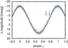 |
Fig. 4 Light variations of KIC 249660366. The solid blue line denotes a fit by the spot model of Prvák (2019). The blue arrows correspond to the phases when the spectra in Table 1 were taken. |
Wavelengths (in Å) of the strongest lines used for KIC 249660366 abundance determination.
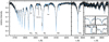 |
Fig. 5 Comparison of observed (black line) and best fit synthetic (blue line) spectra of KIC 249660366. The inset in the right plot shows selected He I lines. The vertical and horizontal scales of the inset are 0.05, and 1 Å, respectively. |
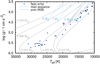 |
Fig. 6 Location of KIC 249660366 in log g – Teff diagram (blue cross). Overplotted are the main-sequence evolutionary tracks (Ekström et al. 2012), post-red giant branch evolutionary tracks (Hall et al. 2013), and the parameters of the blue horizontal branch stars from NGC 6752 (Moni Bidin et al. 2007; Moehler et al. 2017). |
5 Conclusions
We studied the photometric variability of the two K2 targets KIC 250152017 and KIC 249660366 to test the rotational modulation and the nature of the light curves. We derived phase-resolved spectroscopy of both stars and determined parameters from spectroscopic analysis as a function of rotational phase. The selected stars were included among white dwarfs observed by the Kepler satellite (Hermes et al. 2017), but we have shown that neither star is a white dwarf.
Star KIC 250152017 shows an overabundance of the heavy elements titanium, manganese, yttrium, and mercury, and an underabundance of helium, carbon, magnesium, and silicon. These are typical features of HgMn (CP3) stars that appear due to processes of selective radiative force and gravitational settling. The phase-resolved spectroscopy of KIC 250152017 reveals variations of titanium, manganese, and iron lines, which are consistent with their rotational origin. Surface abundance spots of manganese and iron are able to explain the rotational variability of the star. This is the second well-documented study on the nature of light variability of HgMn stars after Prvák et al. (2020).
KIC 249660366 is helium-poor star that shows an overabundance of silicon and argon, low mass, and high gravity corresponding to horizontal branch stars. The peculiar abundance could be also attributed to diffusion processes. Although the phase coverage of the spectra does not allow for a detailed study of spectral variability, the analysis shows that the reflection effect due to the unseen companion provides the most likely explanation of the light variability of this system, which we expect to be of post-common envelope type.
Acknowledgements
The authors thank Dr. Ernst Paunzen for his comments. This research was supported by grant GA ČR 18-05665S. MS acknowledges the financial support of the Operational Program Research, Development and Education – Project Postdoc@MUNI (No. CZ.02.2.69/0.0/0.0/16_027/0008360). This paper includes data collected by the K2 mission. Funding for the K2 mission is provided by the NASA Science Mission directorate. Computational resources were supplied by the project “e-Infrastruktura CZ” (e-INFRA LM2018140) provided within the program Projects of Large Research, Development and Innovations Infrastructures.
Appendix A Fit of the Kepler instrumental profile
We fit to the instrument response curve derived from the Kepler Instrument Handbook (Van Cleve & Caldwell 2016) by a curve
![\begin{equation*} \Phi(\lambda)=\left\{\begin{array}{cl} \exp\left\{{-x^2\left[{a_0+x^4c_0}\right]}\right\}, & x<0,\\[2pt] \exp\left\{{-x^2\left[{a_1+x^2(b_1+x^2c_1)}\right]}\right\}, & x\geq0,\\ \end{array}\right. \end{equation*}](/articles/aa/full_html/2020/07/aa37953-20/aa37953-20-eq6.png) (A.1)
(A.1)


The fit gives precision better than 10%.
References
- Adelman, S. J., Gulliver, A. F., Kochukhov, O. P., & Ryabchikova, T. A. 2002, ApJ, 575, 449 [NASA ADS] [CrossRef] [Google Scholar]
- Aret, A., & Sapar, A. 2002, Astron. Nachr., 323, 21 [CrossRef] [Google Scholar]
- Asplund, M., Grevesse, N., Sauval, A. J., & Scott, P. 2009, ARA&A, 47, 481 [NASA ADS] [CrossRef] [Google Scholar]
- Balona, L. A., Pigulski, A., De Cat, P., et al. 2011, MNRAS, 413, 2403 [NASA ADS] [CrossRef] [Google Scholar]
- Bayo, A., Rodrigo, C., Barrado Y Navascués, D., et al. 2008, A&A, 492, 277 [NASA ADS] [CrossRef] [EDP Sciences] [Google Scholar]
- Briquet, M., Korhonen, H., González, J. F., Hubrig, S., & Hackman, T. 2010, A&A, 511, A71 [NASA ADS] [CrossRef] [EDP Sciences] [Google Scholar]
- Brott, I., de Mink, S. E., Cantiello, M., et al. 2011, A&A, 530, A115 [NASA ADS] [CrossRef] [EDP Sciences] [Google Scholar]
- Budaj, J. 2011, AJ, 141, 59 [NASA ADS] [CrossRef] [Google Scholar]
- Byrne, C. M., & Jeffery, C. S. 2020, MNRAS, 492, 232 [CrossRef] [Google Scholar]
- Castelli, F. 2005, Mem. Soc. Astron. It. Suppl., 8, 25 [Google Scholar]
- Charpinet, S., Fontaine, G., Brassard, P., & Dorman, B. 1996, ApJ, 471, L103 [NASA ADS] [CrossRef] [PubMed] [Google Scholar]
- Dupuis, J., Chayer, P., Vennes, S., Christian, D. J., & Kruk, J. W. 2000, ApJ, 537, 977 [NASA ADS] [CrossRef] [Google Scholar]
- Edelmann, H., Heber, U., Hagen, H. J., et al. 2003, A&A, 400, 939 [NASA ADS] [CrossRef] [EDP Sciences] [Google Scholar]
- Ekström, S., Georgy, C., Eggenberger, P., et al. 2012, A&A, 537, A146 [NASA ADS] [CrossRef] [EDP Sciences] [Google Scholar]
- Flower, P. J. 1996, ApJ, 469, 355 [NASA ADS] [CrossRef] [Google Scholar]
- Gaia Collaboration (Prusti, T., et al.) 2016, A&A, 595, A1 [NASA ADS] [CrossRef] [EDP Sciences] [Google Scholar]
- Gaia Collaboration (Brown, A. G. A., et al.) 2018, A&A, 616, A1 [NASA ADS] [CrossRef] [EDP Sciences] [Google Scholar]
- Geier, S. 2013, A&A, 549, A110 [NASA ADS] [CrossRef] [EDP Sciences] [Google Scholar]
- Ghazaryan, S., Alecian, G., & Hakobyan, A. A. 2018, MNRAS, 480, 2953 [NASA ADS] [CrossRef] [Google Scholar]
- Ghazaryan, S., Alecian, G., & Hakobyan, A. A. 2019, MNRAS, 487, 5922 [CrossRef] [Google Scholar]
- Green, G. M., Schlafly, E. F., Finkbeiner, D., et al. 2018, MNRAS, 478, 651 [NASA ADS] [CrossRef] [Google Scholar]
- Gvaramadze, V. V., Langer, N., Fossati, L., et al. 2017, Nat. Astron., 1, 0116 [NASA ADS] [CrossRef] [Google Scholar]
- Hall, P. D., Tout, C. A., Izzard, R. G., & Keller, D. 2013, MNRAS, 435, 2048 [NASA ADS] [CrossRef] [Google Scholar]
- Harmanec, P. 1988, Bull. astr. Inst. Czechosl., 39, 329 [Google Scholar]
- Hartoog, M. R. 1979, ApJ, 231, 161 [NASA ADS] [CrossRef] [Google Scholar]
- Heber, U. 2016, PASP, 128, 082001 [NASA ADS] [CrossRef] [Google Scholar]
- Hermes, J. J., Gänsicke, B. T., Kawaler, S. D., et al. 2017, ApJS, 232, 23 [NASA ADS] [CrossRef] [Google Scholar]
- Hosek, Matthew W., J., Kudritzki, R.-P., Bresolin, F., et al. 2014, ApJ, 785, 151 [NASA ADS] [CrossRef] [Google Scholar]
- Howell, S. B., Sobeck, C., Haas, M., et al. 2014, PASP, 126, 398 [NASA ADS] [CrossRef] [Google Scholar]
- Hu, H., Tout, C. A., Glebbeek, E., & Dupret, M.-A. 2011, MNRAS, 418, 195 [NASA ADS] [CrossRef] [Google Scholar]
- Hubrig, S., Savanov, I., Ilyin, I., et al. 2010, MNRAS, 408, L61 [NASA ADS] [CrossRef] [Google Scholar]
- Hümmerich, S., Paunzen, E., & Bernhard, K. 2016, AJ, 152, 104 [NASA ADS] [CrossRef] [Google Scholar]
- Hümmerich, S., Niemczura, E., Walczak, P., et al. 2018, MNRAS, 474, 2467 [NASA ADS] [CrossRef] [Google Scholar]
- Johnson, D. R. H., & Soderblom, D. R. 1987, AJ, 93, 864 [NASA ADS] [CrossRef] [Google Scholar]
- Kawka, A., & Vennes, S. 2011, A&A, 532, A7 [NASA ADS] [CrossRef] [EDP Sciences] [Google Scholar]
- Kawka, A., & Vennes, S. 2016, MNRAS, 458, 325 [CrossRef] [Google Scholar]
- Kawka, A., Pigulski, A., O’Toole, S., et al. 2012, ASP Conf. Ser., 452, 121 [Google Scholar]
- Khalack, V. 2018, MNRAS, 477, 882 [CrossRef] [Google Scholar]
- Kilkenny, D., Koen, C., O’Donoghue, D., & Stobie, R. S. 1997, MNRAS, 285, 640 [Google Scholar]
- Kochukhov, O., & Wade, G. A. 2010, A&A, 513, A13 [NASA ADS] [CrossRef] [EDP Sciences] [Google Scholar]
- Kochukhov, O., Adelman, S. J., Gulliver, A. F., & Piskunov, N. 2007, Nat. Phys., 3, 526 [NASA ADS] [CrossRef] [Google Scholar]
- Korhonen, H., González, J. F., Briquet, M., et al. 2013, A&A, 553, A27 [NASA ADS] [CrossRef] [EDP Sciences] [Google Scholar]
- Krtička, J. 2016, A&A, 594, A75 [NASA ADS] [CrossRef] [EDP Sciences] [Google Scholar]
- Krtička, J., & Štefl, V. 1999, A&AS, 138, 47 [NASA ADS] [CrossRef] [EDP Sciences] [Google Scholar]
- Krtička, J., Mikulášek, Z., Zverko, J., & Žižňovský, J. 2007, A&A, 470, 1089 [NASA ADS] [CrossRef] [EDP Sciences] [Google Scholar]
- Krtička, J., Mikulášek, Z., Lüftinger, T., & Jagelka, M. 2015, A&A, 576, A82 [NASA ADS] [CrossRef] [EDP Sciences] [Google Scholar]
- Krtička, J., Janík, J., Krtičková, I., et al. 2019, A&A, 631, A75 [NASA ADS] [CrossRef] [EDP Sciences] [Google Scholar]
- Kurucz, R. L. 2005, Mem. Soc. Astron. It. Suppl., 8, 14 [Google Scholar]
- Landstreet, J. D., & Borra, E. F. 1978, ApJ, 224, L5 [NASA ADS] [CrossRef] [Google Scholar]
- Landstreet, J. D., Bagnulo, S., Fossati, L., Jordan, S., & O’Toole, S. J. 2012, A&A, 541, A100 [NASA ADS] [CrossRef] [EDP Sciences] [Google Scholar]
- Landstreet, J. D., Bagnulo, S., Martin, A., & Valyavin, G. 2016, A&A, 591, A80 [NASA ADS] [CrossRef] [EDP Sciences] [Google Scholar]
- Lanz, T., & Hubeny, I. 2007, ApJS, 169, 83 [CrossRef] [Google Scholar]
- Leone, F., & Lanzafame, A. C. 1997, A&A, 320, 893 [NASA ADS] [Google Scholar]
- Lueftinger, T., Kuschnig, R., Piskunov, N. E., & Weiss, W. W. 2003, A&A, 406, 1033 [NASA ADS] [CrossRef] [EDP Sciences] [Google Scholar]
- Luri, X., Brown, A. G. A., Sarro, L. M., et al. 2018, A&A, 616, A9 [NASA ADS] [CrossRef] [EDP Sciences] [Google Scholar]
- Maitzen, H. M. 1984, A&A, 138, 493 [NASA ADS] [Google Scholar]
- Makaganiuk, V., Kochukhov, O., Piskunov, N., et al. 2011, A&A, 529, A160 [NASA ADS] [CrossRef] [EDP Sciences] [Google Scholar]
- Michaud, G., Tarasick, D., Charland, Y., & Pelletier, C. 1983, ApJ, 269, 239 [NASA ADS] [CrossRef] [Google Scholar]
- Michaud, G., Richer, J., & Richard, O. 2011, A&A, 529, A60 [NASA ADS] [CrossRef] [EDP Sciences] [Google Scholar]
- Mikulášek, Z. 2016, Contrib. Astron. Observ. Skalnate Pleso, 46, 95 [Google Scholar]
- Moehler, S., Dreizler, S., LeBlanc, F., et al. 2017, A&A, 605, C4 [CrossRef] [EDP Sciences] [Google Scholar]
- Molnar, M. R. 1973, ApJ, 179, 527 [NASA ADS] [CrossRef] [Google Scholar]
- Moni Bidin, C., Moehler, S., Piotto, G., Momany, Y., & Recio-Blanco, A. 2007, A&A, 474, 505 [NASA ADS] [CrossRef] [EDP Sciences] [Google Scholar]
- Morel, T., Briquet, M., Auvergne, M., et al. 2014, A&A, 561, A35 [NASA ADS] [CrossRef] [EDP Sciences] [Google Scholar]
- Németh, P., Kawka, A., & Vennes, S. 2012, MNRAS, 427, 2180 [NASA ADS] [CrossRef] [Google Scholar]
- Niemczura, E., Murphy, S. J., Smalley, B., et al. 2015, MNRAS, 450, 2764 [NASA ADS] [CrossRef] [Google Scholar]
- Niemczura, E., Hümmerich, S., Castelli, F., et al. 2017, Sci. Rep., 7, 5906 [NASA ADS] [CrossRef] [Google Scholar]
- Østensen, R. H., Silvotti, R., Charpinet, S., et al. 2010, MNRAS, 409, 1470 [NASA ADS] [CrossRef] [Google Scholar]
- Paunzen, E., Wraight, K. T., Fossati, L., et al. 2013, MNRAS, 429, 119 [NASA ADS] [CrossRef] [Google Scholar]
- Paunzen, E., Bernhard, K., Hümmerich, S., et al. 2019, A&A, 622, A77 [NASA ADS] [CrossRef] [EDP Sciences] [Google Scholar]
- Peterson, D. M. 1970, ApJ, 161, 685 [NASA ADS] [CrossRef] [Google Scholar]
- Pietrukowicz, P., Dziembowski, W. A., Latour, M., et al. 2017, Nat. Astron., 1, 0166 [NASA ADS] [CrossRef] [Google Scholar]
- Piskunov, N., & Kochukhov, O. 2002, A&A, 381, 736 [NASA ADS] [CrossRef] [EDP Sciences] [Google Scholar]
- Preston, G. W. 1974, ARA&A, 12, 257 [NASA ADS] [CrossRef] [MathSciNet] [Google Scholar]
- Prvák, M. 2019, PhD thesis, Masaryk University, Brno, Czechia [Google Scholar]
- Prvák, M., Liška, J., Krtička, J., Mikulášek, Z., & Lüftinger, T. 2015, A&A, 584, A17 [NASA ADS] [CrossRef] [EDP Sciences] [Google Scholar]
- Prvák, M., Krtička, J., & Korhonen, H. 2020, MNRAS, 492, 1834 [CrossRef] [Google Scholar]
- Reindl, N., Bainbridge, M., Przybilla, N., et al. 2019, MNRAS, 482, L93 [NASA ADS] [CrossRef] [Google Scholar]
- Rusomarov, N., Kochukhov, O., Ryabchikova, T., & Piskunov, N. 2015, A&A, 573, A123 [NASA ADS] [CrossRef] [EDP Sciences] [Google Scholar]
- Ryabchikova, T. 1998, Contrib. Astron. Observ. Skalnate Pleso, 27, 319 [NASA ADS] [Google Scholar]
- Ryabchikova, T., Kochukhov, O., & Bagnulo, S. 2008, A&A, 480, 811 [NASA ADS] [CrossRef] [EDP Sciences] [Google Scholar]
- Sargent, A. W. L. W., & Jugaku, J. 1961, ApJ, 134, 777 [NASA ADS] [CrossRef] [Google Scholar]
- Schaffenroth, V., Barlow, B. N., Geier, S., et al. 2019, A&A, 630, A80 [NASA ADS] [CrossRef] [EDP Sciences] [Google Scholar]
- Schneider, F. R. N., Langer, N., de Koter, A., et al. 2014, A&A, 570, A66 [NASA ADS] [CrossRef] [EDP Sciences] [Google Scholar]
- Shultz, M. E., Wade, G. A., Rivinius, T., et al. 2018, MNRAS, 475, 5144 [NASA ADS] [Google Scholar]
- Shulyak, D., Krtička, J., Mikulášek, Z., Kochukhov, O., & Lüftinger, T. 2010, A&A, 524, A66 [CrossRef] [EDP Sciences] [Google Scholar]
- Sikora, J., David-Uraz, A., Chowdhury, S., et al. 2019, MNRAS, 487, 4695 [CrossRef] [Google Scholar]
- Stift, M. J., & Alecian, G. 2012, MNRAS, 425, 2715 [NASA ADS] [CrossRef] [Google Scholar]
- Strassmeier, K. G., Granzer, T., Mallonn, M., Weber, M., & Weingrill, J. 2017, A&A, 597, A55 [NASA ADS] [CrossRef] [EDP Sciences] [Google Scholar]
- Torres, G. 2010, AJ, 140, 1158 [NASA ADS] [CrossRef] [Google Scholar]
- Townsend, R. H. D., Owocki, S. P., & Groote, D. 2005, ApJ, 630, L81 [NASA ADS] [CrossRef] [Google Scholar]
- Tylenda, R., Hajduk, M., Kamiński, T., et al. 2011, A&A, 528, A114 [NASA ADS] [CrossRef] [EDP Sciences] [Google Scholar]
- Unglaub, K., & Bues, I. 2000, A&A, 359, 1042 [NASA ADS] [Google Scholar]
- Unglaub, K., & Bues, I. 2001, A&A, 374, 570 [NASA ADS] [CrossRef] [EDP Sciences] [Google Scholar]
- Valyavin, G., Bagnulo, S., Fabrika, S., et al. 2006, ApJ, 648, 559 [NASA ADS] [CrossRef] [Google Scholar]
- Van Cleve, J. E., & Caldwell, D. A. 2016, Kepler Instrument Handbook, Technical Report [Google Scholar]
- VandenBerg, D. A., Richard, O., Michaud, G., & Richer, J. 2002, ApJ, 571, 487 [NASA ADS] [CrossRef] [EDP Sciences] [Google Scholar]
- Vauclair, S., Dolez, N., & Gough, D. O. 1991, A&A, 252, 618 [NASA ADS] [Google Scholar]
- Vernet, J., Dekker, H., D’Odorico, S., et al. 2011, A&A, 536, A105 [NASA ADS] [CrossRef] [EDP Sciences] [Google Scholar]
- Walczak, P., Fontes, C. J., Colgan, J., Kilcrease, D. P., & Guzik, J. A. 2015, A&A, 580, L9 [NASA ADS] [CrossRef] [EDP Sciences] [Google Scholar]
- White, R. E., Vaughan, A. H., J., Preston, G. W., & Swings, J. P. 1976, ApJ, 204, 131 [NASA ADS] [CrossRef] [Google Scholar]
- Woolf, V. M., & Lambert, D. L. 1999, ApJ, 521, 414 [NASA ADS] [CrossRef] [EDP Sciences] [Google Scholar]
- Zverko, J., Žižňovský, J., & Khokhlova, V. L. 1997, Contrib. Astron. Observ. Skalnate Pleso, 27, 41 [NASA ADS] [Google Scholar]
- Zverko, J., Žižňovský, J., Mikulášek, Z., & Iliev, I. K. 2007, Contrib. Astron. Observ. Skalnate Pleso, 37, 49 [NASA ADS] [Google Scholar]
K2 photometry was obtained from the MAST archive http://archive.stsci.edu, Howell et al. (2014).
The Bonn Stellar Astrophysics Interface web service is available at https://www.astro.uni-bonn.de/stars/bonnsai
All Tables
Derived mean parameters of the studied stars compared to solar abundances (Asplund et al. 2009).
Wavelengths (in Å) of the strongest lines used for KIC 250152017 abundance determination.
Wavelengths (in Å) of the strongest lines used for KIC 249660366 abundance determination.
All Figures
|
Fig. 1 Comparison of observed (black line) and best fit synthetic (blue line) spectra of KIC 250152017. |
| In the text | |
|
Fig. 2 Phase variations of KIC 250152017. Upper panel: K2 magnitudes. The solid line denotes a light curve simulated assuming surface abundance spots of manganese and iron corresponding to the observed spectral variations. Bottom panel: relative variations of abundances. Uncertainties were determined following Hosek et al. (2014). |
| In the text | |
|
Fig. 3 Relative magnitude differences between flux at 6000 Å calculated with enhanced abundance of a given element and flux at KIC 250152017 abundances. |
| In the text | |
|
Fig. 4 Light variations of KIC 249660366. The solid blue line denotes a fit by the spot model of Prvák (2019). The blue arrows correspond to the phases when the spectra in Table 1 were taken. |
| In the text | |
|
Fig. 5 Comparison of observed (black line) and best fit synthetic (blue line) spectra of KIC 249660366. The inset in the right plot shows selected He I lines. The vertical and horizontal scales of the inset are 0.05, and 1 Å, respectively. |
| In the text | |
|
Fig. 6 Location of KIC 249660366 in log g – Teff diagram (blue cross). Overplotted are the main-sequence evolutionary tracks (Ekström et al. 2012), post-red giant branch evolutionary tracks (Hall et al. 2013), and the parameters of the blue horizontal branch stars from NGC 6752 (Moni Bidin et al. 2007; Moehler et al. 2017). |
| In the text | |
Current usage metrics show cumulative count of Article Views (full-text article views including HTML views, PDF and ePub downloads, according to the available data) and Abstracts Views on Vision4Press platform.
Data correspond to usage on the plateform after 2015. The current usage metrics is available 48-96 hours after online publication and is updated daily on week days.
Initial download of the metrics may take a while.