| Issue |
A&A
Volume 683, March 2024
|
|
|---|---|---|
| Article Number | A110 | |
| Number of page(s) | 12 | |
| Section | Stellar atmospheres | |
| DOI | https://doi.org/10.1051/0004-6361/202347359 | |
| Published online | 12 March 2024 | |
The nature of medium-period variables on the extreme horizontal branch
I. X-shooter study of variable stars in the globular cluster ω Cen★
1
Department of Theoretical Physics and Astrophysics, Faculty of Science, Masaryk University,
Kotlářská 2,
Brno, Czech Republic
e-mail: Krticka@physics.muni.cz
2
Instituto de Astronomía, Universidad Católica del Norte,
Av. Angamos,
0610
Antofagasta, Chile
3
INAF – Padova Observatory,
Vicolo dell’Osservatorio 5,
35122
Padova, Italy
4
Universidad Andres Bello, Facultad de Ciencias Exactas, Departamento de Ciencias Físicas – Instituto de Astrofisica,
Autopista Concepción-Talcahuano,
7100
Talcahuano, Chile
Received:
4
July
2023
Accepted:
3
January
2024
A fraction of the extreme horizontal branch stars of globular clusters exhibit a periodic light variability that has been attributed to rotational modulation caused by surface spots. These spots are believed to be connected to inhomogeneous surface distribution of elements. However, the presence of such spots has not been tested against spectroscopic data. We analyzed the phase-resolved ESO X-shooter spectroscopy of three extreme horizontal branch stars that are members of the globular cluster ω Cen and also display periodic light variations. The aim of our study is to understand the nature of the light variability of these stars and to test whether the spots can reproduce the observed variability. Our spectroscopic analysis of these stars did not detect any phase-locked abundance variations that are able to reproduce the light variability. Instead, we revealed the phase variability of effective temperature and surface gravity. In particular, the stars show the highest temperature around the light maximum. This points to pulsations as a possible cause of the observed spectroscopic and photometric variations. However, such an interpretation is in a strong conflict with Ritter’s law, which relates the pulsational period to the mean stellar density. The location of the ω Cen variable extreme horizontal branch stars in HR diagram corresponds to an extension of PG 1716 stars toward lower temperatures or blue, low-gravity, large-amplitude pulsators toward lower luminosities, albeit with much longer periods. Other models of light variability, namely, related to temperature spots, should also be tested further. The estimated masses of these stars in the range of 0.2–0.3 M⊙ are too low for helium-burning objects.
Key words: stars: abundances / stars: horizontal-branch / stars: oscillations / globular clusters: individual: ω Cen
© The Authors 2024
 Open Access article, published by EDP Sciences, under the terms of the Creative Commons Attribution License (https://creativecommons.org/licenses/by/4.0), which permits unrestricted use, distribution, and reproduction in any medium, provided the original work is properly cited.
This article is published in open access under the Subscribe to Open model. Subscribe to A&A to support open access publication.
1 Introduction
A class of main sequence stars, called chemically peculiar stars, shows an unusual type of light variability connected to the presence of surface spots (Hümmerich et al. 2016; Sikora et al. 2019). These spots appear as a result of elemental diffusion, whereby certain elements diffuse upwards under the influence of radiative force, while others sink down as a result of gravitational pull (Vick et al. 2011; Alecian & Stift 2017; Deal et al. 2018). Moderated by the magnetic field (and also by some additional processes, perhaps), surface inhomogeneities appear (Kochukhov & Ryabchikova 2018; Jagelka et al. 2019). The inhomogeneous surface elemental distribution, together with the stellar rotation, leads to periodic spectrum variability. Additionally, the flux redistribution that is due to bound-bound (line) and bound-free (ionization) processes modulated by the stellar rotation causes photometric variability (Peterson 1970; Trasco 1972; Molnar 1973; Lanz et al. 1996). Based on abundance maps from spectroscopy, we see that this effect is able to reproduce the observed rotational light variability of chemically peculiar stars (Prvák et al. 2015; Krtička et al. 2020b).
Besides the radiative diffusion, chemically peculiar stars show other very interesting phenomena, including magneto-spheric radio emission (Leto et al. 2021; Das et al. 2022), trapping of matter in circumstellar magnetosphere (Landstreet & Borra 1978; Townsend & Owocki 2005), magnetic braking (Townsend et al. 2010), and torsional variations (Mikulášek et al. 2011). However, up to now, such phenomena seems to be strictly confined to classical chemically peculiar stars, which inhabit a relatively wide strip on the main sequence with effective temperatures of about 7000–25 000 K.
Therefore, it is highly desirable to search for other types of stars that show similar phenomena. The most promising candidates are stars that have signatures of radiative diffusion in their surface abundances, such as hot horizontal branch stars (Unglaub 2008; Michaud et al. 2011) and hot white dwarfs (Chayer et al. 1995; Unglaub & Bues 2000). Indeed, variations of helium to hydrogen number density ratio have been found on the surface of white dwarfs (Heber et al. 1997; Caiazzo et al. 2023) and some extremely hot white dwarfs even show signatures of corotating magnetospheres (Reindl et al. 2019) and spots (Reindl et al. 2023).
The phenomena connected with chemically peculiar stars can be most easily traced by periodic photometric light variability. However, while there are some signatures of chemical spots in white dwarfs all along their cooling track (Dupuis et al. 2000; Kilic et al. 2015; Reindl et al. 2019), the search for light variability in field horizontal branch stars with Teff < 11 000 K has turned out to be unsuccessful (Paunzen et al. 2019). The prospect of rotationally variable hot subdwarfs was further marred by the discovery of a handful of hot subd-warfs which, despite their detectable surface magnetic fields (Dorsch et al. 2022), still do not show any light variability (Pelisoli et al. 2022).
This perspective changed with the detection of possible rotationally variable hot horizontal branch stars of globular clusters by Momany et al. (2020). However, the presence of abundance spots was anticipated from photometry without any support from spectroscopy. Therefore, we started an observational campaign aiming at detection of abundance spots on these stars and understanding this type of variability overall. Here, we present the results derived for members of ω Cen (NGC 5139).
Spectra used for the analysis.
2 Observations and their analysis
We obtained the spectra of supposed rotational variables in NGC 5139 within the European Southern Observatory (ESO) proposal 108.224V. The spectra were acquired with the X-shooter spectrograph (Vernet et al. 2011) mounted on the 8.2m Melipal (UT3) telescope and these observations are summarized in Table 1. The spectra were obtained with the UVB and VIS arms providing an average spectral resolution (R = λ/∆λ) of 5400 and 6500, respectively. Although medium-resolution spec-trograph is not an ideal instrument for abundance analysis, the abundance determination is typically based on multiple strong lines of given elements. This mitigates the disadvantages of the medium-resolution spectra and enables us to estimate reliable abundances (e.g., Kawka & Vennes 2016; Gvaramadze et al. 2017). In turn, the use of a medium-resolution spectrograph implies a lower number of elements that can be studied and also worsens the precision with respect to the abundance determinations in cases of spectral blends. We extracted the calibrated spectra from the ESO archive. The radial velocity was determined by means of a cross-correlation using the theoretical spectrum as a template (Zverko et al. 2007) and the spectra were shifted to the rest frame.
The stellar parameters were determined using the simplex minimization (Krtička & Štefl 1999) in three steps. First, we determined the effective temperature, Teff, and the surface gravity, log ɡ, by fitting each of the observed spectra with spectra derived from the BSTAR2006 grid of NLTE1 plane parallel model atmospheres with Z/Z⊙ = 0.1 (Lanz & Hubeny 2007). For the present purpose, the grid was extended for models with log ɡ = 5. The random errors of Teff and log ɡ for individual observations were determined by fitting a large set of artificial spectra derived from observed spectra by the addition of random noise with a Gaussian distribution. The dispersion of noise was determined by the signal-to-noise ratio (S/N) (Table 1).
We then estimated surface abundances using the model atmosphere from the grid located closest to the mean of derived parameters. The abundance determination was repeated once more using NLTE plane parallel model atmospheres calculated with TLUSTY200 (Lanz & Hubeny 2003, 2007) for parameters derived in the previous steps. To determine the abundances, we matched the synthetic spectra calculated by SYNSPEC49 code with observed spectra. The random errors of abundances for individual observations were also determined by fitting of artificial spectra derived by adding random noise to the observed spectra. For elements whose abundances were not derived from spectra, we assumed a typical ω Cen abundance log(Z/Z⊙) = −1.5 (Moehler et al. 2011; Moni Bidin et al. 2012). The spectral lines used for the abundance analysis are listed in Table 2. The final parameters averaged over individual spectra are given in Table 3. The derived individual elemental abundances are expressed relative to hydrogen εel = log(nel/nH). Random errors given in Table 3 were estimated from parameters derived from the fits of individual spectra.
Wavelengths (in Å) of the strongest lines used for abundance determinations.
3 Analysis of individual stars
3.1 Star vEHB-2
Our analysis of the spectra for the star vEHB-2 (listed in Table 1) revealed periodic changes in surface gravity and effective temperature (see Fig. 1). To test their presence and any possible correlations, we fixed either the surface gravity or effective temperature and repeated the fit to determine the missing parameter. The test revealed a similar variability of the effective temperature and surface gravity as derived from the fit of both parameters and has not shown any significant change of the derived parameters. Neither one of the parameters determined from individual spectra with added random noise showed any strong correlations. Thus, we conclude that the detected variations of surface gravity and effective temperature are real. We did not detect any strong phase variations of elemental abundances or radial velocities (Sects. 5.2 and 5.3).
Table 3 lists derived parameters of vEHB-2 averaged over the available spectra. The abundances of many elements is slightly higher than a typical ω Cen composition log(Z/Z⊙) = −1.5 (Moehler et al. 2011; Moni Bidin et al. 2012). The exceptions are helium, which is strongly underabundant as a result of gravitational settling, and iron, whose overabundance can be interpreted as a result of radiative diffusion (Unglaub & Bues 2001; Michaud et al. 2011).
With V = 17.249 mag (Momany et al. 2020), E(B − V) = 0.115 ± 0.004 mag (Moni Bidin et al. 2012), the bolometric correction of Flower (1996, see also Torres 2010) BC = −2.40 ± 0.12mag, and distance modulus (m − M)0 = 13.75 ± 0.13 mag (van de Ven et al. 2006), the estimated luminosity is L = 40 ± 7 L⊙. With determined atmospheric parameters this gives the stellar radius 0.34 ± 0.05 R⊙ and mass 0.27 ± 0.11 M⊙. Derived effective temperature is slightly lower than the estimate 28 200 ± 1600 K of Moehler et al. (2011), while our results agree with their surface gravity, log ɡ = 4.86 ± 0.18, and helium abundance, log εHe = −3.20 ± 0.16.
Derived parameters of the studied stars.
3.2 Star vEHB-3
The spectral analysis of vEHB-3 also revealed phase-locked variability of the effective temperature and surface gravity (Fig. 2). The star is hotter and shows higher surface gravity during the light maximum. The analysis of individual spectra has not revealed any significant variations of the radial velocity (Sect. 5.3).
A detailed inspection of spectra shows that the strength of helium lines is variable. This can be most easily seen in He I 4026 and 4471 Å lines (Sect. 6.3). in principle, such variability may also reflect the temperature variations. To test this, for this star we determined abundances for actual temperature and surface gravity derived from individual spectra and not just for the mean values. Even with this modified approach the helium abundance variations has not disappeared, showing that simple effective temperature and gravity variations cannot reproduce the variability of helium lines. We have not detected any strong variability of the line strengths of other elements (Sect. 5.2).
For vEHB-3, Momany et al. (2020) gives V = 17.274 mag, while the mean reddening is E(B − V) = 0.115 ± 0.004 mag (Moni Bidin et al. 2012), the bolometric correction of Flower (1996) is BC = −2.00 ± 0.13 mag, and the distance modulus is (m − M)0 = 13.75 ± 0.13 mag (van de Ven et al. 2006); this results in the luminosity of L = 27 ± 5 L⊙. With the determined atmospheric parameters, this gives a stellar radius of 0.39 ± 0.06 R⊙ and mass of 0.25 ± 0.08 M⊙.
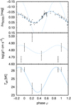 |
Fig. 1 Phase variations of vEHB-2. Upper panel: observed light variations from Momany et al. (2020). Dashed blue line denotes predictions deduced purely from temperature variations, while solid line denotes a fit with additional sinusoidal radius variations. Middle panel: surface gravity variations. Dashed blue line denotes surface gravity determined from the radius variations. Lower panel: effective temperature variations. Solid blue line denotes sinusoidal fit. Part of the variations for φ < 0 and φ > 1 are repeated for better visibility. |
3.3 Star vEHB-7
In total, five spectra for vEHB-7 were obtained. However, one of them is of a poor quality and an additional spectrum was marred by a wrong pointing. Consequently, there are just three spectra left. Anyway, the analysis of these spectra indicates presence of temperature variations (Fig. 3), with temperature maximum appearing around the time of light maximum. The available spectra do not show any strong variability of surface abundances nor the radial velocities (Sects. 5.2 and 5.3).
The V magnitude of the star is V = 17.644 mag (Momany et al. 2020), which with the reddening E(B − V) = 0.115 ± 0.004 mag (Moni Bidin et al. 2012), the bolometric correction of Flower (1996) BC = −2.02 ± 0.07 mag, and distance modulus (m − M)0 = 13.75 ± 0.13 mag (van de Ven et al. 2006) gives a luminosity of L = 20 ± 3 L⊙. With the atmospheric parameters determined from spectroscopy, this gives a stellar radius of 0.33 ± 0.03 R⊙ and mass of 0.20 ± 0.04 M⊙. The star was analyzed by Latour et al. (2018), who derived slightly higher effective temperature of 23800 ± 800K, surface gravity of log ɡ = 5.11 ± 0.06, and mass of 0.49 ± 0.10 M⊙.
4 Significance of the detected variations
Before discussing the implications of the detected variations for the mechanism of the light variability of the stars, we first need to clarify whether the detected variations could be real. To this end, we used a random number generator to create a population of stellar parameters with dispersions determined from the uncertainty of each measurement in each phase. We compared the dispersion of the derived artificial population with the dispersion of the derived data and determined a fraction of the population that gives a higher dispersion than the data determined from observation. if this fraction is high, then it is likely that the derived variations are only sampling random noise.
For the effective temperature, the derived fraction is lower than 10−5 for all three stars. The uncertainties of estimated effective temperatures should be a factor of three higher to reach a fraction of 0.01 for vEHB-7 − and even higher for the remaining stars. Thus, we conclude that the detected variations of the effective temperature are very likely to be real for all the stars studied here.
The same is true for the variations of the surface gravity, where the uncertainties should by a factor of 1.6 higher to reach a fraction of 0.01 for vEHB-7. From this, we conclude that also the variations of the surface gravity are very likely real in vEHB-2 and vEHB-3, with a small chance that the gravity variations in vEHB-7 are random.
5 Nature of the light variations
5.1 Pulsations
We detected a variability among the effective temperature and surface gravity phased with photometric variations in all studied stars (Figs. 1–3). The effective temperature and surface gravity are typically the highest during the maximum of the light variability. in the absence of any strong radial velocity variations (Sect. 5.3), such changes in the stellar parameters can be most naturally interpreted as resulting from the pulsations (e.g., Woolf & Jeffery 2002; Fossati et al. 2014; Vasilyev et al. 2018).
To test the pulsational origin of the light variability, we calculated the synthetic light curves and compared it with observed light variability. As a first step, we used the fluxes from the BSTAR2006 database calculated for Z = 0.1 Z⊙ and log ɡ = 4.75, convolved them with the response function of uSDSS, and fitted them as a function of the effective temperature, deriving:

The fit is valid between Teff = 15–30 kK. We fit the observational phase variations of the effective temperature by a simple sinusoidal (plotted in Figs. 1–3) and used these variations to predict the light variations (dashed curve in the upper plots of Figs. 1–3). The prediction assumes that the temperature is the sameacross the stellar surface, corresponding to the radial pulsations. The resulting light variations have always higher amplitude than the observed light curve, but this can be attributed to radius variations. We searched for such sinusoidal radius variations that would allow us to reproduce the observed light variations. it turns out that radius variations with amplitudes of about few percent and phase-shifted by nearly half period from temperature variations are fully able to reproduce the observed light variations (solid line in the upper panels of Figs. 1–3). Assuming that the pulsating atmosphere is roughly in hydrostatic equilibrium, the effective surface gravity varies due to a change in radius and as a result of inertial force. This is plotted using the dashed curve in the middle plot of Figs. 1–3. The resulting amplitude of the surface gravity variations is always comparable to the observed variations, albeit the curves are in good agreement only for vEHB-3.
The fact that the resulting phase variations of surface gravity do not fully agree with observations is understandable for several reasons. The spectroscopy was obtained just in few phases, which makes the effective temperature phase curve rather uncertain. Moreover, the width of the line profiles is affected by the electron number density and not directly by the surface gravity. The dependence of the line profiles on gravity stems from the hydrostatic equilibrium equation. However, the equation of hydrostatic equilibrium can be violated in pulsating stars, especially in the presence of shocks (Jeffery et al. 2022). Additionally, the effective temperature determined from spectroscopy may not correspond to temperature of radiation emerging from the continuum formation region. Finally, contrary to our assumption, the stars may experience non-radial pulsations, further complicating the analysis.
Pulsating stars often show relation between period and luminosity (e.g., Leavitt 1908; Freedman & Madore 1990; Mowlavi et al. 2016) which stems from the dependence of pulsational period on mean stellar density or sound wave crossing time. it is worthy to notice that in Table 3 the more luminous stars have longer periods. On average, the period-luminosity relationship can be expressed as (see Fig. 4):

However, the analysis involves strong selection effect, because we have focused on brightest stars from the Momany et al. (2020) sample.
The pulsational hypothesis can be further tested using ultraviolet photometric variations (e.g., Krtička et al. 2023), which should correspond to optical variations. The amplitude of the radial velocity variations due to proposed pulsational motion is of the order 0.1 km s−1. Therefore, the presence of pulsations can be also tested using precise radial velocity measurements.
However, the interpretation of observed light variations in terms of pulsations poses a challenge for pulsational theory. Field hot subdwarfs typically pulsate with frequencies that are one to two orders of magnitude higher than found here (Østensen et al. 2012; Jeffery et al. 2017; Baran et al. 2021). This stems from Ritter’s law (Ritter 1879), which predicts that the period of pulsations is inversely proportional to the square root of the mean stellar density. As a result, tenuous cool giants and super-giants pulsate with periods of the order of hundreds of days (Ahmad et al. 2023). On the other hand, the p-modes of relatively high-density hot subdwarfs are predicted to have periods of the order of hundreds of seconds (Guo 2018). With typical pulsational constants (Lesh & Aizenman 1974; Saio & Gautschy 1998), Ritter’s law gives a period of the order of hundredths of a day for studied stars, which is three orders of magnitude lower than the period of variability of studied stars. The beating of two close periods could lead to variability with longer period, but it remains unclear how the short periods could be damped in surface regions. The g-modes may have longer periods (Miller Bertolami et al. 2020) and would thus serve as better candidates for explaining the observed periodic light variability.
The period of g-mode pulsations depends on the buoyancy oscillation travel time across the corresponding resonance cavity (Garcia et al. 2022). The related Brunt-Väisälä frequency approaches zero when the radiative temperature gradient is close to the adiabatic gradient. Hot stars possess an iron convective zone, which disappears for low iron abundances (Jermyn et al. 2022). However, the studied stars show relatively high iron abundance as a result of radiative diffusion (Table 3). Therefore, it is possible that interplay of the radiative diffusion and proximity to the convection instability may lead to the appearance of medium-period pulsations.
The pulsations may not necessarily be driven by classical κ-mechanism. The location of studied stars in log ɡ − Teff diagram corresponds to stars experiencing helium subflashes before the helium-core burning phase (Battich et al. 2018). Such stars are predicted to have pulsations driven by the ϵ-mechanism.
If the light variations are indeed due to pulsations, then the stars could be analogues of other pulsating subdwarfs, as the EC 14026 stars (Kilkenny et al. 1997) and PG 1159 stars (GW Vir stars, Córsico et al. 2008), however, with much longer periods. Taking into account the derived stellar parameters, the location of the variables from ω Cen in HR diagram corresponds to the extension of PG 1716 stars (Green et al. 2003) toward lower effective temperatures. Stellar parameters of studied stars are also close to the blue large-amplitude pulsators (Pietrukowicz et al. 2017), which are somehow more luminous and slightly hotter. The search for pulsations in corresponding cluster stars was, to our knowledge, not successful (Reed et al. 2006); surprisingly, only significantly hotter pulsating stars were detected on the horizontal branch (Randall et al. 2011; Brown et al. 2013). The studied stars are located in area of Hertzsprung-Russell diagram (HRD), where pulsations resulting from the κ-mechanism on the iron-bump opacity can be expected; however, with significantly shorter periods (Charpinet et al. 1996; Jeffery & Saio 2006, 2016). The pulsational instability appears at high iron abundances, which are also detected in studied stars.
Pulsating subdwarfs typically evince non-radial pulsations (Córsico et al. 2008), for which low amplitudes of photometric variations are expected. Still, Kupfer et al. (2019) detected a new class of variable stars corresponding to blue, high-gravity, large-amplitude pulsators that are pulsating radially with amplitudes that are comparable to the stars studied here.
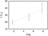 |
Fig. 4 Period-luminosity relationship for studied stars. Dashed line corresponds to the linear fit. |
5.2 Abundance spots
As one of the possible mechanisms behind the detected light variability, Momany et al. (2020) suggested the rotational flux modulation due to abundance spots. Any light variability modulated by rotation requires that the rotational velocity determined from the period of variability and stellar radius should be higher than the rotational velocity projection, υrot sin i, determined from spectroscopy. However, the spectroscopy provides only a very loose constraint on the rotational velocities of individual stars, υrot sin i < 50 km s−1. As a result, with the stellar radii (from Table 3) and photometric periods (listed in Table 1) determined by Momany et al. (2020), the rotational modulation of photometric variability cannot be ruled out. Therefore, the test of abundance spots requires a more elaborate approach.
In principle, determination of light curves due to abundance spots from the observed spectroscopy is a straightforward procedure. The inverse method of Doppler imaging is used to determine surface abundance maps (e.g., Kochukhov et al. 2022). From the derived abundance maps, the light curves can be simulated using model atmospheres synthetic spectra (e.g., Krtička et al. 2020b). However, the Doppler imaging requires relatively large number of high-resolution and high S/N spectra. With the current instrumentation, this is beyond the reach of even 8-m class telescopes. Therefore, another method has to be used to test the presence of surface spots.
For faint stars, it is possible to estimate surface abundances as a function of phase and simulate the light variability directly from derived abundances (Krtička et al. 2020a). However, the observations do not suggest the presence of abundance spots on the surface of the stars. There is some scatter of abundances derived from individual spectra, but the potential abundance variations are not correlated with light variations. This can be seen from Fig. 5, where we plot the abundances derived from individual spectra as a function of observed magnitude (both values are plotted with respect to the mean). If the light variations were due to the abundance variations, the plot should evince a positive correlation between abundance and magnitudes (Prvák et al. 2015; Krtička et al. 2020b), but such a correlation is missing. Moreover, the amplitude of abundance variations (which is no more than about 0.1 dex) should be one magnitude higher to cause observed light variations (c.f., Oksala et al. 2015; Krtička et al. 2020b). On top of that, the mean abundance should be high enough to affect the emergent flux.
We additionally tested the abundance spot model of the light variability using model atmosphere emergent fluxes. We calculated the model atmospheres with ten times higher abundances of helium, silicon, and iron than those determined from spectroscopy. This is an order of magnitude higher overabundance than observations allow. We calculated the magnitude difference between the fluxes corresponding to enhanced and observational abundances in the uSDSS band used by Momany et al. (2020). This gives a theoretical upper limit of the magnitude of the light variability. In the case of helium and silicon, the derived amplitude of the light variability would be 0.002 and 0.02 mag, which is significantly lower than the observed amplitude of the light variability. The amplitude is higher only in the case of iron (0.4 mag), but even in this case the maximum iron abundance does not appear during the maximum of the light curve (Fig. 5). Moreover, the detected abundance variations can be interpreted in terms of random fluctuations.
There is a possibility that the variations are caused by ele-ment(s) that do not appear in the optical spectra. However, this is unlikely, because in classical chemically peculiar stars the abundance variations are not confined just to a single element (e.g., Rusomarov et al. 2018; Kochukhov et al. 2022). Consequently, we conclude that derived abundance variations from individual spectra are most likely of statistical origin. Therefore, the studied stars do not likely show light variability due to surface spots similar to main sequence, chemically peculiar stars.
The only element that varies with magnitude is helium (Fig. 5), but it shows opposite behavior than is required to explain the light variability due flux redistribution. This means that the helium lines are observed to be stronger during the light minimum. Moreover, the helium line profiles are complex and we were unable to reasonably fit the observed helium lines using synthetic spectra. Therefore, instead of spots, we suspect that they are formed by intricate motions in the atmosphere during pulsations (Sect. 6.3).
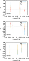 |
Fig. 5 Difference between abundances of selected elements derived from individual spectra and a mean abundance. Plotted as a function of relative magnitudes for individual stars. Elements plotted in the graph typically contribute most significantly to the light variations at studied effective temperatures (Oksala et al. 2015; Krtička et al. 2020b). The individual points were shifted slightly horizontally to avoid overlapping. |
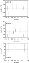 |
Fig. 6 Phase variations of radial velocity determined from individual spectra with respect to the mean value. Plotted for individual stars. Parts of the variations for φ < 0 and φ > 1 repeat for a better visibility. |
5.3 Binary origin
It may be possible that the observed light variations are due to binary effects. in that case, there would be a number of combinations for the arrangement of the system. it is unlikely that the variations are due to the reflection effect on a cooler companion, because in such cases, the system would look cooler during the light maxima, which would contradict the observations. Moreover, the predicted amplitude would be too low. Due to the absence of any strong radial velocity variations (Fig. 6) and for evolutionary reasons, the cooler companion would be less massive; from this (and the third Kepler law), the resulting binary separation would be about 11 R⊙ for vEHB-2 (and even lower for remaining stars). This once more precludes the assumption of the red giant as a companion and leaves just enough space for a low-mass main sequence star. Furthermore, we used our code calculating light curves due to the reflection effect, which predicts that the radius of such a star should be comparable to solar radius to cause observed light variations. Therefore, for low-mass main sequence star, the light amplitude would be significantly lower than observed.
The reflection due to a hotter companion is constrained by the absence of strong companion lines in the optical spectra and by missing large radial velocity variations (Fig. 6). This leaves two options, both involving hot (possibly degenerated) companion. Either the companion has low mass (possibly implying a hot helium white dwarf) or the system involves high-mass companion on an orbit with low inclination. In any case, given a typical mass of extreme horizontal branch stars (Moni Bidin et al. 2007, 2012) and maximum mass of white dwarfs (Yoshida 2019; Nunes et al. 2021), it is unlikely that the total mass of the system exceeds 2 M⊙. In this case the Kepler third law predicts an orbital separation of a = 21 R⊙ for vEHB-2. From the Saha-Boltzmann law, the required temperature of irradiating body is ![${T_{{\rm{irr}}}} = \sqrt {{a \mathord{\left/ {\vphantom {a {{R_{{\rm{irr}}}}}}} \right. \kern-\nulldelimiterspace} {{R_{{\rm{irr}}}}}}} {\left[ {2\left( {T_2^4 - T_1^4} \right)} \right]^{{1 \mathord{\left/ {\vphantom {1 4}} \right. \kern-\nulldelimiterspace} 4}}}$](/articles/aa/full_html/2024/03/aa47359-23/aa47359-23-eq3.png) , where Rirr is the radius of irradiating body and T2 and T1 are the maximum and minimum temperatures of studied star. With a typical radius of a white dwarf Rirr = 0.01 R⊙ this gives Tirr = 106 K, far exceeding the temperature of any white dwarf (Miller Bertolami 2016). This estimate could be decreased assuming a lower mass of irradiating body and excluding the detected radius variations, but it still amounts to about 300 kK for the star vEHB-7 with the shortest period. From this, we conclude that it is unlikely that the observed light variations are caused by binary companion.
, where Rirr is the radius of irradiating body and T2 and T1 are the maximum and minimum temperatures of studied star. With a typical radius of a white dwarf Rirr = 0.01 R⊙ this gives Tirr = 106 K, far exceeding the temperature of any white dwarf (Miller Bertolami 2016). This estimate could be decreased assuming a lower mass of irradiating body and excluding the detected radius variations, but it still amounts to about 300 kK for the star vEHB-7 with the shortest period. From this, we conclude that it is unlikely that the observed light variations are caused by binary companion.
We subsequently performed a similar analysis as done by Moni Bidin et al. (2006, 2009) and searched for binarity from the radial velocity data. From the analysis, it follows that the measurements are perfectly compatible with constant radial velocities. A Kolmogorov-Smirnov test reveals that the probability of these results being drawn from a normal distribution (with a dispersion equal to the observational errors) is equal or higher than about 50% for each star (namely 48, 64, and 86% for vEHB-2, vEHB-3, and vEHB-7).
Going further, we estimated the probability of these stars being undetected binaries. The most common close companions of extreme horizontal branch stars are compact objects such as white dwarfs. Hence, we simulated systems of 0.49 + 0.49 M⊙ stars (typical of such systems), in circular orbits (because the short periods suggest a previous common envelope phase, which circularizes the orbits), with orbital period equal to the photometric one, an isotropic distribution of the angle of inclination of the orbit (hence uniform in sin i), and a random phase. We considered a system to be “undetected” if the observed radial velocities (at the epochs of observations) show a maximum variation lower or equal to that observed. We found that the probability that the studies stars hide undetected binary are 1.74% for vEHB-2, 0.68% for vEHB-3, and <0.01% for vEHB-7. The differences stem from different periods of variability. In conclusion, the angle of inclination cannot explain the lack of evidence with respect to binarity.
For the radial velocity analysis, we assumed a canonical mass for the extreme horizontal branch stars, but the estimated values are much lower. The lower mass would make the probabilities even lower, because with a smaller mass, the radial velocity variations would be greater. On the other hand, with lower mass of the companion, the binarity could pass undetected more easily. Consequently, we checked what the companion mass must be to obtain the probability of an undetected binary of at least 5%. This results in 0.27, 0.17, and 0.04M⊙ for the studied stars. As we have already shown, the masses are too low to explain photometric variations by mean of ellipsoidal variation or reflection effects. The exception could possibly be vEHB-2, but it has the longest period, which implies a much larger separation between the components, again arguing against both tidal and reflection effects.
Another possibility is that the light variations are not due to the star itself, but due to another star that coincidentally appears at the same location on the sky. However, it is difficult to find such types of variable stars that would correspond to observations. Pulsating stars of RR Lyr type, which are indeed found on horizontal branch of globular clusters, have significantly shorter periods (e.g., Skarka et al. 2020; Molnár et al. 2022). The period of variability better corresponds to Cepheids. Type II Cepheids may correspond to low-mass stars that left the horizontal branch (Bono et al. 2020) and are indeed found in globular clusters (Braga et al. 2020). However, they are much brighter in the visual domain than stars studied here. On the other hand, classical Cepheids corresponds to blue loops on evolutionary tracks of stars that are more massive than appear in globular clusters now (Neilson et al. 2016). This would imply a distant background object that is younger than the cluster. However, taking into account the fact that extreme horizontal branch stars constitute just a very small fraction of cluster stars, we consider a chance alignment in three of them to be very unlikely.
5.4 Temperature spots
Momany et al. (2020) pointed out that the observed photometric variations could be caused by temperature spots. Such spots are predicted to be caused by shallow subsurface convective zones that may be present in hot stars (Cantiello & Braithwaite 2011, 2019) and connected to surface magnetic fields. This could indicate the presence of either a He II or deeper Fe convective zone. However, helium is significantly underabundant in studied stars and a corresponding region of helium underabundance may extend deep into the star (Michaud et al. 2011). As a result, the He II convection zone may be absent (Quievy et al. 2009), as indicated also by our evolutionary models (Sect. 6.4).
The studied variability seems to be stable on a timescale of years, while the subsurface convection zones were invoked to explain variability that is more stochastic in nature (Cantiello et al. 2021) and has a significantly lower amplitude. Subsurface convection was suggested to drive corotating interacting regions in hot star winds (David-Uraz et al. 2017), which require more spatially coherent structures, but it is unclear whether they are persistent in the course of hundreds of days. Based on the analogy with cool star spots and considering photometric observations of hot stars (Chené et al. 2011; Ramiaramanantsoa et al. 2014; Aerts et al. 2018), we consider this possibility to be unlikely. Moreover, the iron convective zone appears directly beneath the stellar surface, therefore, it does not seem likely that the magnetic fields can cause large variations of stellar radius (c.f., Fuller & Mathis 2023).
We have detected variations of the effective temperature (Figs. 1–3), but they predict a greater amplitude of light variability than what has been observed. To reduce the amplitude, we introduced additional variations of radius, which cause variability of surface gravity. The detected variations of surface gravity are in conflict with models of temperature spots. We tested this by fitting synthetic spectra derived from combination of spectra with different effective temperatures, but the same surface gravities. This should mimic the spectra of a star with temperature spot(s). The fit provided an effective temperature between the temperatures of combined spectra, but the surface gravity remained nearly constant and equal to the surface gravities of individual spectra.
About one-third of stars with spots show complex light curves with a double-wave structure (Jagelka et al. 2019). However, all the light curves observed by Momany et al. (2020) are much simpler and consist of just a single wave. This also is an argument against the notion of spots causing the photometric variability of the studied stars.
The model of temperature spots can be further observationally tested using spectropolarimetry, which should be able to detect accompanying weak magnetic fields. Hot spots could be also detected from radial velocity variations, which should show a minimum at about a quarter of a phase before the light maximum. This phase variability is opposite to radial velocity variations due to pulsations, which show a maximum at a quarter phase before the light maximum.
6 Discussion
6.1 Stellar masses
Stellar masses of studied stars derived from spectroscopy and photometry are rather low for single core-helium burning objects. Although the uncertainties are typically very large, the masses are systematically lower than a canonical mass of isolated subdwarfs (Heber 2016). Comparable mass problems also appear in other studies of globular cluster horizontal branch stars with similar temperatures (Moni Bidin et al. 2012; Moehler et al. 2019; Latour et al. 2023).
The cause of this problem is unclear (see the discussion in Moni Bidin et al. 2011). With a fixed surface gravity from spectroscopy, a higher mass requires larger radius. This can be achieved either by significantly lower V magnitude, higher distance modulus, higher reddening, or lower bolometric correction. A lower apparent magnitude is unlikely. The Gaia distance modulus of ω Cen is slightly lower than the value adopted here (Soltis et al. 2021) worsening the problem even more. The adopted reddening agrees with independent estimations (Calamida et al. 2005; Bono et al. 2019). The bolometric corrections might be uncertain and, indeed, Lanz & Hubeny (2007) reported slightly lower value than adopted here. However, this alone would not solve the problem. Our analysis using the model atmosphere fluxes computed here, with the help of Eq. (1) from Lanz & Hubeny (2007), shows that a lower helium abundance slightly increases the bolometric correction, thus worsening the discrepancy once again.
This leaves the uncertainties of parameter determinations from spectroscopy as the only remaining cause of overly low derived masses of studied stars connected with the analysis. The true uncertainties could be higher than the random errors (given in Table 3) when accounting for systematic errors (Sect. 6.5).
Lower mass subdwarfs may also originate due to some more exotic evolutionary processes. Subdwarfs with mass lower than the canonical one are found among field stars, but they typically appear in binaries (Kupfer et al. 2017) and require binary interaction for explanation (Althaus et al. 2013). Moreover, stars with initial masses of about 2 M⊙ may ignite helium in a nondegenerate core with mass as low as 0.32 M⊙ (Han et al. 2002; Arancibia-Rojas et al. 2024). However, the lifetime of such stars is at odds with expected age of ω Cen. in any case, low-mass white dwarfs with mass around 0.2 M⊙ were detected, which are considered to be connected with hot subdwarfs (Heber 2016). A lower mass of about 0.3 M⊙ was also predicted for blue large-amplitude pulsators in the context of their He pre-white dwarf nature (Córsico et al. 2018; Romero et al. 2018). However, alternative models for these stars propose either helium shell or core burning subdwarfs with higher masses (Wu & Li 2018; Xiong et al. 2022).
6.2 Tension with parameters from literature
For star vEHB-7, Latour et al. (2018) determined slightly higher effective temperature and surface gravity. However, their data were collected by the FORS spectrograph, which has a lower resolution that X-shooter. We simulated the consequences of using low resolution spectra for the derived parameters and we smoothed the data by a Gaussian filter with dispersion of 3 Å, which roughly corresponds to a FORS resolution, according to the user manual2. The fitting of spectra with a lower resolution has systematically provided higher effective temperatures by about 500 K and higher surface gravities by about 0.2 dex. This partially explains the differences in the derived parameters.
Similarly, Moehler et al. (2011) found a higher effective temperature for vEHB-2. However, these authors used spectra with shorter interval of wavelengths. Our tests have shown that this can lead to differences in the effective temperature of about 1000 K and surface gravity of about 0.1 dex. This could be one of the reasons behind the differences in the determined parameters.
The effective temperature and surface gravity were derived from the fits of models with underabundances of heavier elements, although we do see that iron shows an overabundance with respect to the solar value (Table 3). Moehler et al. (2000) alleviated this problem by using models with higher abundances of iron. However, the comparison of spectra from the BSTAR2006 grid (Lanz & Hubeny 2007), with different iron abundances, showed nearly identical hydrogen line profiles. Therefore, we conclude that this is not a significant problem for the parameter determination presented here.
Two of the variable horizontal branch stars detected by Momany et al. (2020) in NGC 6752 were subsequently analyzed by Latour et al. (2023). it turned out than only one of them is a genuine horizontal branch star, while the other was instead classified as a blue straggler. The horizontal branch star has very similar atmospheric parameters as obtained here and it also has a slightly lower mass than typical for horizontal branch stars (Fig. 14, Latour et al. 2023), albeit higher than that derived here.
6.3 Line variability
We detected variability among the helium and calcium lines, which is also likely to be phased with the variability period (Figs. 7 and 8). Such variability may indicate presence of spots. However, our tests have shown that the abundances are too low to cause any significant light variability (Sect. 5.2). Classical chemically peculiar stars may show vertical abundance gradients in the atmosphere (e.g., LeBlanc et al. 2009; Khalack 2018), but this would not help to explain the light variability because the opacity in the continuum-forming region is decisive. Moreover, the line profiles are unusually broad in some cases and the calcium line may even appear in the emission. This is the case for the star vEHB-2 (Fig. 8). in addition, emission is also likely to appear in one spectrum of vEHB-7, which was not included in the present analysis due to its low S/N.
The unusual variability of these lines and the appearance of emission could be perhaps connected with shocks that propagate throughout the stellar atmosphere as a result of pulsational motion (Schwarzschild et al. 1948; Jeffery et al. 2022). The shock may possibly heat the atmosphere and induce the emission in the Ca II 3934 Å line. The shock appears around the phase of minimum radius (maximum gravity), which agrees with spectroscopy of vEHB-2 (Fig. 8).
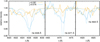 |
Fig. 7 Comparison of observed (solid lines) and predicted (dashed lines) helium line profiles for two different phases in the spectra of vEHB-3. |
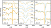 |
Fig. 8 Phase variability of Ca II 3934 Å line. Plotted for individual studied stars for all phases (denoted in the graph). The plot compares observed spectra (yellow lines) with predicted spectra (blue lines). The vertical scale denotes fraction of the continuum intensity. The spectra were shifted to the stellar rest frame. |
6.4 Evolutionary considerations
To better constrain the nature of the light variability of the studied stars, we simulated their internal structure using the MESA code3 (Paxton et al. 2019; Jermyn et al. 2023). We selected a model star with an initial mass of 2.2 M⊙, which starts to burn helium at the moment when the core mass is close to the mass of the stars used in this study (Han et al. 2002).
We simulated the evolution of a star from the pre-main sequence until the initiation of helium-burning in the core. By setting the mass fraction of heavy elements to Z = 0.0006 and incorporating convective premixing and the Ledoux criterion4, we ensured a similar representation of the stellar conditions. Compared to standard models, we also included silicon and iron elements to account for the essential constituents found from observations. Afterward, we stripped the star’s envelope, leaving behind only the helium-core enveloped by a hydrogen-rich outer layer with mass of 0.01 M⊙. This process allowed us to imitate the physical structure found in horizontal branch stars. We also evolved a similar model star with an additional accreted mass of 0.001 M⊙ mirroring the composition of the surface material deduced in vEHB-2.
Our approach is similar to the work of Han et al. (2002) and gives comparable effective temperatures (25-30 kK) and surface gravities (log ɡ ≈ 5.5) during the helium-burning phase. Contrary to Han et al. (2002), who were able to create the lowest mass helium-burning star with a zero-age main sequence mass of 1.8 M⊙ for Z = 0.004, we found that our models did not allow us to use such a low initial mass. This suggests that compactness of the inner core was greatly affected by including the heavy elements, thereby creating helium or hydrogen flashes for lower initial masses.
We noticed a notable disparity between the non-accreted and accreted models. While the models with near solar helium fraction (Y = 0.24) displayed a convection layer near the surface, the layer disappeared after the accretion of helium-poor material. Therefore, models do not predict any subsurface convective region for a chemical composition derived from observations.
Alternatively, the parameters of the stars correspond to stars in the post-red giant evolutionary state (Hall et al. 2013). In that case, the variability of studied stars could be connected with instability of hydrogen-burning on the surface of a degenerate core (Shen & Bildsten 2007), which could lead to periodic behavior (Jose et al. 1993).
6.5 Random and systematic errors
Random errors among the parameters in individual phases were determined using the Monte Carlo method. However, there might be certain errors in the analysis that could not be described by random errors. To better assess the statistical significance of the results, we searched the ESO X-shooter archive for multiple observations of subdwarfs. We focused on subdwarfs listed in the catalog from Geier (2020), which have similar parameters to those of the horizontal branch stars studied here.
We selected the field hot subdwarf EC 01510-3919, which has four spectra from two nights available in total. We analyzed the spectra in the same way as we did for horizontal branch stars. The analysis provided Teff = 20440 ± 90 K and log ɡ = 4.73 ± 0.02, in a good agreement with parameters determined by Lisker et al. (2005).
The maximum differences between effective temperature and surface gravity estimates from individual spectra were about 200 K and 0.03 dex, respectively. Although the S/N of the spectra is roughly a factor of two higher than for globular cluster stars, this further demonstrates that the detected variations of the effective temperature and surface gravity are likely to be real. Moreover, the analysis also shows that the mismatch between observed and fitted variations of surface gravity of vEHB-7 could be of a random origin.
We studied the effect of continuum normalization on the uncertainty of parameters. To test the influence of normalization, we multiplied the absolute data by a smooth function and repeated the analysis again (including normalization). This had a small effect on the derived parameters. We performed additional tests by restricting the number of lines used for the analysis. This also led to similar variations as those we detected, albeit with a larger scatter.
Unlike the random errors considered here, the systematic errors are much more difficult to estimate. They may be connected with uncertainties of parameters such as oscillator strengths, NLTE model ions, continuum placement, and selection of lines for the analysis (Przybilla et al. 2000).
The systematic errors can be roughly estimated from a comparison of derived parameters with independent estimates from the literature, which gives an error of about 1000 K in the effective temperature, and 0.1 dex in the surface gravity and abundances. However, unlike the random errors, the systematic errors affect all the measurements in approximately the same way. Therefore, because this study is focused mainly on the origin of the light variability connected to differences among individual spectra, the systematic errors are of a lesser importance.
7 Conclusions
We analyzed the phase-resolved spectroscopy of three periodically variable extreme horizontal branch stars from the globular cluster ω Cen that were detected by Momany et al. (2020). We determined the effective temperatures, surface gravities, and abundances in individual photometric phases.
We detected the phase variability of the apparent effective temperature and surface gravity. The effective temperature is the highest during the light maximum. We did not detect any strong variability of abundances that could explain the observed photometric variations; neither did we detect any significant radial velocity variations that could point to the binarity. Instead, the photometric and spectroscopic variability can be interpreted in terms of pulsations. This is additionally supported by the anomalous profiles of helium and calcium lines that point to intricate atmospheric motions. The effective temperatures of these stars, 21–25 kK, and the surface gravity correspond to extension of PG 1716 stars or blue, high-gravity, large-amplitude pulsators toward lower temperatures, albeit with much longer periods. Given the effective temperature of these stars and the length of their periods, we propose that the pulsation of these stars are due to g modes initiated by the iron opacity bump. However, the length of the periods of the order of day is in strong conflict with Ritter’s law.
Surface temperature spots provide the only viable alternative explanation for the light variability. Nevertheless, the detection of surface gravity variations in studied stars and the existence of complex line profile variations of the helium and calcium lines offer additional support for the pulsational model.
The metal-deficient chemical composition of these stars corresponds to the horizontal branch of globular clusters. One exception is iron, with a roughly solar chemical composition that is perhaps due to radiative diffusion. On the other hand, helium has significantly subsolar abundance that is likely due to gravitational settling.
We estimated the masses of these stars from spectroscopy and photometry in the range of 0.2–0.3 M⊙. This value is too low for helium-burning stars, but similar estimates were obtained previously for horizontal branch stars.
Acknowledgements
We thank Dr. Yazan Momany for valuable comments on the paper and Dr. Petr Kurfürst for the discussion. Computational resources were provided by the e-INFRA CZ project (ID:90254), supported by the Ministry of Education, Youth and Sports of the Czech Republic.
References
- Aerts, C., Bowman, D. M., Símon-Díaz, S., et al. 2018, MNRAS, 476, 1234 [NASA ADS] [CrossRef] [Google Scholar]
- Ahmad, A., Freytag, B., & Höfner, S. 2023, A&A, 669, A49 [NASA ADS] [CrossRef] [EDP Sciences] [Google Scholar]
- Alecian, G., & Stift, M. J. 2017, MNRAS, 468, 1023 [Google Scholar]
- Althaus, L. G., Miller Bertolami, M. M., & Córsico, A. H. 2013, A&A, 557, A19 [NASA ADS] [CrossRef] [EDP Sciences] [Google Scholar]
- Arancibia-Rojas, E., Zorotovic, M., Vučković, M., et al. 2024, MNRAS, 527, 11184 [Google Scholar]
- Asplund, M., Grevesse, N., Sauval, A. J., & Scott, P. 2009, ARA&A, 47, 481 [NASA ADS] [CrossRef] [Google Scholar]
- Baran, A. S., Sahoo, S. K., Sanjayan, S., & Ostrowski, J. 2021, MNRAS, 503, 3828 [NASA ADS] [CrossRef] [Google Scholar]
- Battich, T., Miller Bertolami, M. M., Córsico, A. H., & Althaus, L. G. 2018, A&A, 614, A136 [NASA ADS] [CrossRef] [EDP Sciences] [Google Scholar]
- Bono, G., Iannicola, G., Braga, V. F., et al. 2019, ApJ, 870, 115 [NASA ADS] [CrossRef] [Google Scholar]
- Bono, G., Braga, V. F., Fiorentino, G., et al. 2020, A&A, 644, A96 [NASA ADS] [CrossRef] [EDP Sciences] [Google Scholar]
- Braga, V. F., Bono, G., Fiorentino, G., et al. 2020, A&A, 644, A95 [NASA ADS] [CrossRef] [EDP Sciences] [Google Scholar]
- Brown, T. M., Landsman, W. B., Randall, S. K., Sweigart, A. V., & Lanz, T. 2013, ApJ, 777, L22 [NASA ADS] [CrossRef] [Google Scholar]
- Caiazzo, I., Burdge, K. B., Tremblay, P.-E., et al. 2023, Nature, 620, 61 [NASA ADS] [CrossRef] [Google Scholar]
- Calamida, A., Stetson, P. B., Bono, G., et al. 2005, ApJ, 634, L69 [NASA ADS] [CrossRef] [Google Scholar]
- Cantiello, M., & Braithwaite, J. 2011, A&A, 534, A140 [NASA ADS] [CrossRef] [EDP Sciences] [Google Scholar]
- Cantiello, M., & Braithwaite, J. 2019, ApJ, 883, 106 [Google Scholar]
- Cantiello, M., Lecoanet, D., Jermyn, A. S., & Grassitelli, L. 2021, ApJ, 915, 112 [NASA ADS] [CrossRef] [Google Scholar]
- Charpinet, S., Fontaine, G., Brassard, P., & Dorman, B. 1996, ApJ, 471, L103 [Google Scholar]
- Chayer, P., Fontaine, G., & Wesemael, F. 1995, ApJS, 99, 189 [NASA ADS] [CrossRef] [Google Scholar]
- Chené, A. N., Moffat, A. F. J., Cameron, C., et al. 2011, ApJ, 735, 34 [CrossRef] [Google Scholar]
- Córsico, A. H., Althaus, L. G., Kepler, S. O., Costa, J. E. S., & Miller Bertolami, M. M. 2008, A&A, 478, 869 [NASA ADS] [CrossRef] [EDP Sciences] [Google Scholar]
- Córsico, A. H., Romero, A. D., Althaus, L. G., Pelisoli, I., & Kepler, S. O. 2018, ArXiv e-prints [arXiv:1809.07451] [Google Scholar]
- Das, B., Chandra, P., Shultz, M. E., et al. 2022, ApJ, 925, 125 [NASA ADS] [CrossRef] [Google Scholar]
- David-Uraz, A., Owocki, S. P., Wade, G. A., Sundqvist, J. O., & Kee, N. D. 2017, MNRAS, 470, 3672 [NASA ADS] [CrossRef] [Google Scholar]
- Deal, M., Alecian, G., Lebreton, Y., et al. 2018, A&A, 618, A10 [NASA ADS] [CrossRef] [EDP Sciences] [Google Scholar]
- Dorsch, M., Reindl, N., Pelisoli, I., et al. 2022, A&A, 658, L9 [NASA ADS] [CrossRef] [EDP Sciences] [Google Scholar]
- Dupuis, J., Chayer, P., Vennes, S., Christian, D. J., & Kruk, J.W. 2000, ApJ, 537, 977 [NASA ADS] [CrossRef] [Google Scholar]
- Flower, P. J. 1996, ApJ, 469, 355 [NASA ADS] [CrossRef] [Google Scholar]
- Fossati, L., Kolenberg, K., Shulyak, D. V., et al. 2014, MNRAS, 445, 4094 [Google Scholar]
- Freedman, W. L., & Madore, B. F. 1990, ApJ, 365, 186 [NASA ADS] [CrossRef] [Google Scholar]
- Fuller, J., & Mathis, S. 2023, MNRAS, 520, 5573 [CrossRef] [Google Scholar]
- Garcia, S., Van Reeth, T., De Ridder, J., & Aerts, C. 2022, A&A, 668, A137 [NASA ADS] [CrossRef] [EDP Sciences] [Google Scholar]
- Geier, S. 2020, A&A, 635, A193 [NASA ADS] [CrossRef] [EDP Sciences] [Google Scholar]
- Green, E. M., Fontaine, G., Reed, M. D., et al. 2003, ApJ, 583, L31 [Google Scholar]
- Guo, J.-J. 2018, ApJ, 866, 58 [NASA ADS] [CrossRef] [Google Scholar]
- Gvaramadze, V. V., Langer, N., Fossati, L., et al. 2017, Nat. Astron., 1, 0116 [NASA ADS] [CrossRef] [Google Scholar]
- Hall, P. D., Tout, C. A., Izzard, R. G., & Keller, D. 2013, MNRAS, 435, 2048 [Google Scholar]
- Han, Z., Podsiadlowski, P., Maxted, P. F. L., Marsh, T. R., & Ivanova, N. 2002, MNRAS, 336, 449 [Google Scholar]
- Heber, U. 2016, PASP, 128, 082001 [Google Scholar]
- Heber, U., Napiwotzki, R., Lemke, M., & Edelmann, H. 1997, A&A, 324, L53 [Google Scholar]
- Hümmerich, S., Paunzen, E., & Bernhard, K. 2016, AJ, 152, 104 [CrossRef] [Google Scholar]
- Jagelka, M., Mikulášek, Z., Hümmerich, S., & Paunzen, E. 2019, A&A, 622, A199 [NASA ADS] [CrossRef] [EDP Sciences] [Google Scholar]
- Jeffery, C. S., & Saio, H. 2006, MNRAS, 371, 659 [NASA ADS] [CrossRef] [Google Scholar]
- Jeffery, C. S., & Saio, H. 2016, MNRAS, 458, 1352 [NASA ADS] [CrossRef] [Google Scholar]
- Jeffery, C. S., Baran, A. S., Behara, N. T., et al. 2017, MNRAS, 465, 3101 [NASA ADS] [CrossRef] [Google Scholar]
- Jeffery, C. S., Montañés-Rodríguez, P., & Saio, H. 2022, MNRAS, 509, 1940 [Google Scholar]
- Jermyn, A. S., Anders, E. H., & Cantiello, M. 2022, ApJ, 926, 221 [NASA ADS] [CrossRef] [Google Scholar]
- Jermyn, A. S., Bauer, E. B., Schwab, J., et al. 2023, ApJS, 265, 15 [NASA ADS] [CrossRef] [Google Scholar]
- Jose, J., Hernanz, M., & Isern, J. 1993, A&A, 269, 291 [NASA ADS] [Google Scholar]
- Kawka, A., & Vennes, S. 2016, MNRAS, 458, 325 [NASA ADS] [CrossRef] [Google Scholar]
- Khalack, V. 2018, MNRAS, 477, 882 [NASA ADS] [CrossRef] [Google Scholar]
- Kilic, M., Gianninas, A., Bell, K. J., et al. 2015, ApJ, 814, L31 [NASA ADS] [CrossRef] [Google Scholar]
- Kilkenny, D., Koen, C., O’Donoghue, D., & Stobie, R. S. 1997, MNRAS, 285, 640 [Google Scholar]
- Kochukhov, O., & Ryabchikova, T. A. 2018, MNRAS, 474, 2787 [NASA ADS] [CrossRef] [Google Scholar]
- Kochukhov, O., Papakonstantinou, N., & Neiner, C. 2022, MNRAS, 510, 5821 [NASA ADS] [CrossRef] [Google Scholar]
- Krtička, J., & Štefl, V. 1999, A&AS, 138, 47 [NASA ADS] [CrossRef] [EDP Sciences] [Google Scholar]
- Krtička, J., Kawka, A., Mikulášek, Z., et al. 2020a, A&A, 639, A8 [EDP Sciences] [Google Scholar]
- Krtička, J., Mikulášek, Z., Prvák, M., et al. 2020b, MNRAS, 493, 2140 [Google Scholar]
- Krtička, J., Benáček, J., Budaj, J., et al. 2023, Space Science Reviews, submitted [arXiv:2306.15081] [Google Scholar]
- Kupfer, T., Ramsay, G., van Roestel, J., et al. 2017, ApJ, 851, 28 [NASA ADS] [CrossRef] [Google Scholar]
- Kupfer, T., Bauer, E. B., Burdge, K. B., et al. 2019, ApJ, 878, L35 [Google Scholar]
- Landstreet, J. D., & Borra, E. F. 1978, ApJ, 224, L5 [NASA ADS] [CrossRef] [Google Scholar]
- Lanz, T., & Hubeny, I. 2003, ApJS, 146, 417 [NASA ADS] [CrossRef] [Google Scholar]
- Lanz, T., & Hubeny, I. 2007, ApJS, 169, 83 [CrossRef] [Google Scholar]
- Lanz, T., Artru, M. C., Le Dourneuf, M., & Hubeny, I. 1996, A&A, 309, 218 [NASA ADS] [Google Scholar]
- Latour, M., Randall, S. K., Calamida, A., Geier, S., & Moehler, S. 2018, A&A, 618, A15 [NASA ADS] [CrossRef] [EDP Sciences] [Google Scholar]
- Latour, M., Hämmerich, S., Dorsch, M., et al. 2023, A&A, 677, A86 [NASA ADS] [CrossRef] [EDP Sciences] [Google Scholar]
- Leavitt, H. S. 1908, Ann. Harvard College Observ., 60, 87 [Google Scholar]
- LeBlanc, F., Monin, D., Hui-Bon-Hoa, A., & Hauschildt, P. H. 2009, A&A, 495, 93 [Google Scholar]
- Lesh, J. R., & Aizenman, M. L. 1974, A&A, 34, 203 [NASA ADS] [Google Scholar]
- Leto, P., Trigilio, C., Krtička, J., et al. 2021, MNRAS, 507, 1979 [NASA ADS] [CrossRef] [Google Scholar]
- Lisker, T., Heber, U., Napiwotzki, R., et al. 2005, A&A, 430, 223 [NASA ADS] [CrossRef] [EDP Sciences] [Google Scholar]
- Michaud, G., Richer, J., & Richard, O. 2011, A&A, 529, A60 [NASA ADS] [CrossRef] [EDP Sciences] [Google Scholar]
- Mikulášek, Z., Krtička, J., Henry, G. W., et al. 2011, A&A, 534, L5 [NASA ADS] [CrossRef] [EDP Sciences] [Google Scholar]
- Miller Bertolami, M. M. 2016, A&A, 588, A25 [NASA ADS] [CrossRef] [EDP Sciences] [Google Scholar]
- Miller Bertolami, M. M., Battich, T., Córsico, A. H., Christensen-Dalsgaard, J., & Althaus, L. G. 2020, Nat. Astron., 4, 67 [Google Scholar]
- Moehler, S., Sweigart, A. V., Landsman, W. B., & Heber, U. 2000, A&A, 360, 120 [NASA ADS] [Google Scholar]
- Moehler, S., Dreizler, S., Lanz, T., et al. 2011, A&A, 526, A136 [NASA ADS] [CrossRef] [EDP Sciences] [Google Scholar]
- Moehler, S., Landsman, W. B., Lanz, T., & Miller Bertolami, M. M. 2019, A&A, 627, A34 [NASA ADS] [CrossRef] [EDP Sciences] [Google Scholar]
- Molnar, M. R. 1973, ApJ, 179, 527 [NASA ADS] [CrossRef] [Google Scholar]
- Molnár, L., Bódi, A., Pál, A., et al. 2022, ApJS, 258, 8 [CrossRef] [Google Scholar]
- Momany, Y., Zaggia, S., Montalto, M., et al. 2020, Nat. Astron., 4, 1092 [Google Scholar]
- Moni Bidin, C., Moehler, S., Piotto, G., et al. 2006, A&A, 451, 499 [NASA ADS] [CrossRef] [EDP Sciences] [Google Scholar]
- Moni Bidin, C., Moehler, S., Piotto, G., Momany, Y., & Recio-Blanco, A. 2007, A&A, 474, 505 [NASA ADS] [CrossRef] [EDP Sciences] [Google Scholar]
- Moni Bidin, C., Moehler, S., Piotto, G., Momany, Y., & Recio-Blanco, A. 2009, A&A, 498, 737 [NASA ADS] [CrossRef] [EDP Sciences] [Google Scholar]
- Moni Bidin, C., Villanova, S., Piotto, G., Moehler, S., & D’Antona, F. 2011, ApJ, 738, L10 [NASA ADS] [CrossRef] [Google Scholar]
- Moni Bidin, C., Villanova, S., Piotto, G., et al. 2012, A&A, 547, A109 [NASA ADS] [CrossRef] [EDP Sciences] [Google Scholar]
- Mowlavi, N., Saesen, S., Semaan, T., et al. 2016, A&A, 595, L1 [NASA ADS] [CrossRef] [EDP Sciences] [Google Scholar]
- Neilson, H. R., Engle, S. G., Guinan, E. F., Bisol, A. C., & Butterworth, N. 2016, ApJ, 824, 1 [Google Scholar]
- Nunes, S. P., Arbañil, J. D. V., & Malheiro, M. 2021, ApJ, 921, 138 [NASA ADS] [CrossRef] [Google Scholar]
- Oksala, M. E., Kochukhov, O., Krtička, J., et al. 2015, MNRAS, 451, 2015 [Google Scholar]
- Østensen, R. H., Degroote, P., Telting, J. H., et al. 2012, ApJ, 753, L17 [CrossRef] [Google Scholar]
- Paunzen, E., Bernhard, K., Hümmerich, S., et al. 2019, A&A, 622, A77 [NASA ADS] [CrossRef] [EDP Sciences] [Google Scholar]
- Paxton, B., Smolec, R., Schwab, J., et al. 2019, ApJS, 243, 10 [Google Scholar]
- Pelisoli, I., Dorsch, M., Heber, U., et al. 2022, MNRAS, 515, 2496 [NASA ADS] [CrossRef] [Google Scholar]
- Peterson, D. M. 1970, ApJ, 161, 685 [NASA ADS] [CrossRef] [Google Scholar]
- Pietrukowicz, P., Dziembowski, W. A., Latour, M., et al. 2017, Nat. Astron., 1, 0166 [Google Scholar]
- Prvák, M., Liška, J., Krtička, J., Mikulášek, Z., & Lüftinger, T. 2015, A&A, 584, A17 [NASA ADS] [CrossRef] [EDP Sciences] [Google Scholar]
- Przybilla, N., Butler, K., Becker, S. R., Kudritzki, R. P., & Venn, K. A. 2000, A&A, 359, 1085 [NASA ADS] [Google Scholar]
- Quievy, D., Charbonneau, P., Michaud, G., & Richer, J. 2009, A&A, 500, 1163 [NASA ADS] [CrossRef] [EDP Sciences] [Google Scholar]
- Ramiaramanantsoa, T., Moffat, A. F. J., Chené, A.-N., et al. 2014, MNRAS, 441, 910 [NASA ADS] [CrossRef] [Google Scholar]
- Randall, S. K., Calamida, A., Fontaine, G., Bono, G., & Brassard, P. 2011, ApJ, 737, L27 [NASA ADS] [CrossRef] [Google Scholar]
- Reed, M. D., Kilkenny, D., & Terndrup, D. M. 2006, Balt. Astron., 15, 65 [NASA ADS] [Google Scholar]
- Reindl, N., Bainbridge, M., Przybilla, N., et al. 2019, MNRAS, 482, L93 [Google Scholar]
- Reindl, N., Islami, R., Werner, K., et al. 2023, A&A, 677, A29 [NASA ADS] [CrossRef] [EDP Sciences] [Google Scholar]
- Ritter, A. 1879, Annal. Phys., 243, 304 [NASA ADS] [CrossRef] [Google Scholar]
- Romero, A. D., Córsico, A. H., Althaus, L. G., Pelisoli, I., & Kepler, S. O. 2018, MNRAS, 477, L30 [NASA ADS] [CrossRef] [Google Scholar]
- Rusomarov, N., Kochukhov, O., & Lundin, A. 2018, A&A, 609, A88 [NASA ADS] [CrossRef] [EDP Sciences] [Google Scholar]
- Saio, H., & Gautschy, A. 1998, ApJ, 498, 360 [NASA ADS] [CrossRef] [Google Scholar]
- Schwarzschild, M., Schwarzschild, B., & Adams, W. S. 1948, ApJ, 108, 207 [NASA ADS] [CrossRef] [Google Scholar]
- Shen, K. J., & Bildsten, L. 2007, ApJ, 660, 1444 [NASA ADS] [CrossRef] [Google Scholar]
- Sikora, J., David-Uraz, A., Chowdhury, S., et al. 2019, MNRAS, 487, 4695 [Google Scholar]
- Skarka, M., Prudil, Z., & Jurcsik, J. 2020, MNRAS, 494, 1237 [NASA ADS] [CrossRef] [Google Scholar]
- Soltis, J., Casertano, S., & Riess, A. G. 2021, ApJ, 908, L5 [Google Scholar]
- Torres, G. 2010, AJ, 140, 1158 [Google Scholar]
- Townsend, R. H. D., & Owocki, S. P. 2005, MNRAS, 357, 251 [NASA ADS] [CrossRef] [Google Scholar]
- Townsend, R. H. D., Oksala, M. E., Cohen, D. H., Owocki, S. P., & ud-Doula, A. 2010, ApJ, 714, L318 [NASA ADS] [CrossRef] [Google Scholar]
- Trasco, J. D. 1972, ApJ, 171, 569 [NASA ADS] [CrossRef] [Google Scholar]
- Unglaub, K. 2008, A&A, 486, 923 [NASA ADS] [CrossRef] [EDP Sciences] [Google Scholar]
- Unglaub, K., & Bues, I. 2000, A&A, 359, 1042 [NASA ADS] [Google Scholar]
- Unglaub, K., & Bues, I. 2001, A&A, 374, 570 [NASA ADS] [CrossRef] [EDP Sciences] [Google Scholar]
- van de Ven, G., van den Bosch, R. C. E., Verolme, E. K., & de Zeeuw, P. T. 2006, A&A, 445, 513 [NASA ADS] [CrossRef] [EDP Sciences] [Google Scholar]
- Vasilyev, V., Ludwig, H. G., Freytag, B., Lemasle, B., & Marconi, M. 2018, A&A, 611, A19 [NASA ADS] [CrossRef] [EDP Sciences] [Google Scholar]
- Vernet, J., Dekker, H., D’Odorico, S., et al. 2011, A&A, 536, A105 [NASA ADS] [CrossRef] [EDP Sciences] [Google Scholar]
- Vick, M., Michaud, G., Richer, J., & Richard, O. 2011, A&A, 526, A37 [NASA ADS] [CrossRef] [EDP Sciences] [Google Scholar]
- Woolf, V. M., & Jeffery, C. S. 2002, A&A, 395, 535 [NASA ADS] [CrossRef] [EDP Sciences] [Google Scholar]
- Wu, T., & Li, Y. 2018, MNRAS, 478, 3871 [NASA ADS] [CrossRef] [Google Scholar]
- Xiong, H., Casagrande, L., Chen, X., et al. 2022, A&A, 668, A112 [NASA ADS] [CrossRef] [EDP Sciences] [Google Scholar]
- Yoshida, S. 2019, MNRAS, 486, 2982 [NASA ADS] [CrossRef] [Google Scholar]
- Zverko, J., Žižňovský, J., Mikulášek, Z., & Iliev, I. K. 2007, Contrib. Astron. Observ. Skalnate Pleso, 37, 49 [NASA ADS] [Google Scholar]
For reference see https://docs.mesastar.org/en/latest/index.html
All Tables
All Figures
|
Fig. 1 Phase variations of vEHB-2. Upper panel: observed light variations from Momany et al. (2020). Dashed blue line denotes predictions deduced purely from temperature variations, while solid line denotes a fit with additional sinusoidal radius variations. Middle panel: surface gravity variations. Dashed blue line denotes surface gravity determined from the radius variations. Lower panel: effective temperature variations. Solid blue line denotes sinusoidal fit. Part of the variations for φ < 0 and φ > 1 are repeated for better visibility. |
| In the text | |
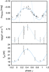 |
Fig. 2 Same as Fig. 1, but for vEHB-3. |
| In the text | |
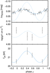 |
Fig. 3 Same as Fig. 1, but for vEHB-7. |
| In the text | |
|
Fig. 4 Period-luminosity relationship for studied stars. Dashed line corresponds to the linear fit. |
| In the text | |
|
Fig. 5 Difference between abundances of selected elements derived from individual spectra and a mean abundance. Plotted as a function of relative magnitudes for individual stars. Elements plotted in the graph typically contribute most significantly to the light variations at studied effective temperatures (Oksala et al. 2015; Krtička et al. 2020b). The individual points were shifted slightly horizontally to avoid overlapping. |
| In the text | |
|
Fig. 6 Phase variations of radial velocity determined from individual spectra with respect to the mean value. Plotted for individual stars. Parts of the variations for φ < 0 and φ > 1 repeat for a better visibility. |
| In the text | |
|
Fig. 7 Comparison of observed (solid lines) and predicted (dashed lines) helium line profiles for two different phases in the spectra of vEHB-3. |
| In the text | |
|
Fig. 8 Phase variability of Ca II 3934 Å line. Plotted for individual studied stars for all phases (denoted in the graph). The plot compares observed spectra (yellow lines) with predicted spectra (blue lines). The vertical scale denotes fraction of the continuum intensity. The spectra were shifted to the stellar rest frame. |
| In the text | |
Current usage metrics show cumulative count of Article Views (full-text article views including HTML views, PDF and ePub downloads, according to the available data) and Abstracts Views on Vision4Press platform.
Data correspond to usage on the plateform after 2015. The current usage metrics is available 48-96 hours after online publication and is updated daily on week days.
Initial download of the metrics may take a while.