| Issue |
A&A
Volume 694, February 2025
|
|
|---|---|---|
| Article Number | A270 | |
| Number of page(s) | 5 | |
| Section | Stellar atmospheres | |
| DOI | https://doi.org/10.1051/0004-6361/202453189 | |
| Published online | 19 February 2025 | |
Horizontal flows in the atmospheres of chemically peculiar stars
1
Penn State Scranton,
120 Ridge View Drive,
Dunmore,
PA
18512,
USA
2
Department of Theoretical Physics and Astrophysics, Masaryk University,
Kotlářská 2,
611 37
Brno,
Czech Republic
3
Astronomical Institute of the Czech Academy of Sciences,
Fričova 298,
251 65
Ondřejov,
Czech Republic
★ Corresponding author; asif@psu.edu
Received:
27
November
2024
Accepted:
22
January
2025
Context. Classical chemically peculiar stars exhibit atmospheres that are often structured by the effects of atomic diffusion. As a result of these elemental diffusion and horizontal abundance variations, the photospheric temperature varies at a given height in the atmosphere. This may lead to horizontal flows in the photosphere. In addition, the suppression of such flows by a magnetic field can alter the elemental transport processes.
Aims. Using a simplified model of such a structured atmosphere and 2D magnetohydrodynamic simulations of a typical He-rich star, we examined atmospheric flows in these chemically peculiar stars, which often are strongly magnetic.
Methods. We used Zeus-MP, which is a publicly available Fortran 90-based parallel finite element modular code.
Results. We find that for non-magnetic stars of spectral type BA, the atmospheric flow related to the horizontal temperature gradient can reach 1.0 km s−1, yielding mixing timescales of the order of tens of days. For the magnetic counterparts, the flow speeds are an order of magnitude lower, allowing for the stratification of chemical elements.
Conclusions. Magnetic fields can significantly influence the dynamics in atmospheres. A strong horizontal magnetic field inhibits flow in the vertical direction, while a strong vertical magnetic field can suppress horizontal atmospheric flow and prevent elemental mixing.
Key words: stars: chemically peculiar / circumstellar matter / stars: early-type / stars: general / stars: magnetic field / stars: variables: general
© The Authors 2025
 Open Access article, published by EDP Sciences, under the terms of the Creative Commons Attribution License (https://creativecommons.org/licenses/by/4.0), which permits unrestricted use, distribution, and reproduction in any medium, provided the original work is properly cited.
This article is published in open access under the Subscribe to Open model. Subscribe to A&A to support open access publication.
1 Introduction
The atmospheres of classical chemically peculiar stars in the upper part of the main sequence are structured by the effects of atomic diffusion under the influence of radiative and gravitational forces (Michaud et al. 2011, 2015; Alecian & Stift 2017). In the absence of strong mixing, this leads to horizontal and vertical abundance stratification in the outer layers of these stars (Kochukhov & Wade 2010; Kochukhov et al. 2011; Ryabchikova et al. 2008).
The outer layers of chemically peculiar stars are frequently stabilized by a strong magnetic field (Morel et al. 2015; Wade et al. 2016; Grunhut et al. 2017). The rotation of the stellar surface strewn with inhomogeneously distributed elements, together with a frozen-in magnetic field, manifests itself in a plethora of remarkable phenomena. These include regular light variability (Faltová et al. 2021; Labadie-Bartz et al. 2023), which stems from the flux frequency redistribution induced by horizontal chemical inhomogeneity (Krtička et al. 2015; Prvák et al. 2015), and radio activity originating from the interaction of a weak stellar wind with a strong magnetic field (Leto et al. 2021; Das et al. 2022; Owocki et al. 2022).
Although many detailed characteristics of chemically peculiar stars can be understood from theoretical models, the processes that shape the elemental distribution of their surface are not fully understood. The diffusion models predict a tight correlation between the surface elemental distribution and magnetic field (Alecian & Stift 2017), which is perhaps only the case for some elements (Kochukhov & Ryabchikova 2018). The observed characteristics of light variations in magnetic chemically peculiar stars do not seem to support a strong correlation between the magnetic field and surface abundance distribution (Jagelka et al. 2019). In particular, simulations of light curves based on abundance spots associated with magnetic fields predict a much higher prevalence of double-wave light curves per rotation period than is observed.
Although the theoretical diffusion models and abundance distributions inferred from observations seem to contradict one another, any additional process that modifies the surface abundance distribution is likely to be rather weak. This is indicated by the stability of the observational characteristics of magnetic chemically peculiar stars. Neither the observed light curves (Hümmerich et al. 2018) nor the underlying surface abundance distribution (Potravnov et al. 2024) seem to show any secular changes. This implies that either the abundance stratification has reached an equilibrium state or that the forming processes operate on a longer timescale (e.g. Alecian et al. 2011).
A better understanding of the diffusion processes can perhaps be gleaned from the analysis of chemically peculiar stars of types Am and HgMn. These stars do not show strong magnetic fields (Makaganiuk et al. 2012; Kochukhov et al. 2013; Catanzaro et al. 2016; Blazère et al. 2020) that would impede the interaction of mixing processes and elemental diffusion, unlike in the magnetic chemically peculiar stars. This is likely the reason why the rotational light variability in HgMn stars is much weaker than in magnetic chemically peculiar stars. As a result, the light variability of a fraction of HgMn stars remained undetected until the age of precise space-borne instruments (Kochukhov et al. 2021). Moreover, the connection between the light variability and surface abundance inhomogeneities is not well established. Despite this, in some of these stars it was possible to detect secular changes in the surface elemental distribution, the origin of which is as yet unknown (Briquet et al. 2010; Korhonen et al. 2013; Prvák et al. 2020).
While the deviations from the axial symmetry of the stellar surface, either due to the magnetic fields (Fuller & Mathis 2023) or to hydrostatic scale-height variations caused by horizontal abundance variations (Krtička et al. 2020), are rather small, other dynamical processes were used to provide additional mixing of the atmospheres of chemically peculiar stars. Such processes can include turbulence and mass loss (Michaud et al. 2011; Alecian & Stift 2019), or meridional circulation (Michaud et al. 1983).
In addition to these processes, there is a possible mixing process directly linked to peculiarity that had not been studied in detail until now. As a result of elemental diffusion and induced horizontal abundance variations, the photospheric temperature varies at a given height in the atmosphere. Such horizontal temperature variations exist regardless of the overall constancy of the effective temperature (Molnar 1973) and appear to be a result of the influence of heavy element abundance on opacity. These temperature variations that occur in the optically thin photospheric layers are rather weak (of the order of 10–100 K), and are related to surface brightness variations and light variability (Khan & Shulyak 2007; Krtička et al. 2007, 2012).
The variation in temperature at a given height within the atmospheres of chemically peculiar stars implies that pressure is likewise non-uniform at the same altitude (e.g. Peterson 1970). In such cases, horizontal pressure differences generate weak lateral flows that are analogous to atmospheric winds on Earth. Given the complex surface abundance patterns in chemically peculiar stars, the resulting flow induced by these pressure gradients represents a complex three-dimensional problem. Numerical modelling of this phenomenon is challenging due to the substantial difference in the horizontal and vertical extents of the flow, with significant disparities in scale making such simulations computationally intensive. Furthermore, the structure of the flow varies from star to star due to unique abundance stratifications across each stellar surface.
To develop a clearer physical understanding of this phenomenon, we employed a simplified model that assumes an initial linear temperature gradient in two dimensions directly over the region of chemical peculiarity. This approach enabled us to estimate the intensity of the pressure-gradient-driven flow while capturing essential dynamics. Additionally, we introduced uniform magnetic fields of different orientations and strengths into our simulations to explore the potential damping effects on these flows, which is particularly relevant in the atmospheres of the chemically peculiar magnetic stars where magnetic suppression of the flow could alter the transport processes.
In Sect. 2 we discuss the specifics of our numerical methods. We then present our results in Sect. 3. We follow this with a brief discussion in Sect. 4 before a short summary and outline of future work in Sect. 5.
2 Numerical methods
To model flows that stem from the horizontal temperature gradients, we set up a ‘box-in-a-star’ simulation of the hydrostatic stellar atmosphere, wherein a chemical spot with varying temperature is mimicked by a region with a temperature ΔT that is higher than the effective temperature Teff of the star.
We used the publicly available hydrodynamic code Zeus-MP (Hayes et al. 2006) to model the atmospheric structure of a chemically peculiar star under a planar approximation. The stellar parameters used in the simulations were chosen to approximate the typical magnetic helium-strong star HD 37776 (Mikulášek et al. 2008), and are as follows: mass M = 8 M⊙, radius R = 4 R⊙, and effective temperature Teff = 22000 K. Although we used a full energy equation for the gas, we assumed the adiabatic index γ = 1.01, which reflects nearly isothermal atmospheric conditions.
We initialized all our simulations with a hydrostatic planar atmosphere that had a fixed gravitational acceleration of  and a base density of ρ* = 10−8 g cm−3. At time t = 0 s we introduced a uniform magnetic field with different strengths and orientations, as noted in Table 1.
We included a temperature variation in the form of a chemical spot, specified as a linear temperature increase of ΔT = 100 K at X = 0, symmetric about X = 0 and spanning 5 Hscale on both sides. Here Hscale = kBT/(µmHɡ) = a2/ɡ is the pressure scale height with an isothermal sound speed of  where µ is the mean molecular weight and mH is the hydrogen mass. For the parameters assumed in this work, the scale height amounts to Hscale ~ 2.1 × 108 cm.
For the horizontal (X) direction, we fixed the density and pressure to the value appropriate for a hydrostatic atmosphere. We also kept the magnetic field components constant. While the horizontal component of the velocity was kept at zero value in the interest of numerical stability, the vertical component was allowed to float through linear extrapolation from the two closest zones inside the computational domain.
At the outer boundary, which represents the upper atmosphere, outflow boundary conditions were implemented, which allowed all magnetohydrodynamic quantities to vary freely. The boundary is located at approximately X = 10 Hscale or about 21000 km above the stellar surface. Reflective boundary conditions were imposed along the vertical (ɀ) direction, corresponding to the left and right sides of the panels in all subsequent figures. Under these conditions, the parallel components of velocity and magnetic field remain unchanged, while the perpendicular components reverse their direction. The computational domain spans a total horizontal extent of 20 Hscale, while the vertical extent is half as large, measuring 10 Hscale. The computational domain was discretized into 128 × 64 grid zones along the x- and ɀ-directions, yielding approximately six to seven grid points per scale height (Hscale). A total of nine models were explored: one non-magnetic reference case and eight magnetic configurations with field strengths of 1, 10, 100, and 1000 G in both horizontal and vertical orientations. Each simulation spans a physical time of 100 ks, which corresponds to over 50 sound crossing times, ensuring adequate time for the system to reach equilibrium.
Models with varying magnetic field strengths and orientations.
3 Simulation results
3.1 Non-magnetic model
To establish a basis for comparison across all magnetic models, we first examined the non-magnetic case (0 G). Figure 1 illustrates the temporal evolution of the non-magnetic model, with panels showing temperature (T; left column), horizontal velocity (υx; middle column), and vertical or radial velocity (υɀ; right column), all in cgs units. Initially, the model was assumed to be in hydrostatic equilibrium along the vertical direction. However, the imposed temperature gradient across the modelled chemical spot quickly generated a horizontal pressure gradient, which initiated lateral flow that facilitated the mixing of cooler and warmer gas regions.
The fixed temperature gradient at the base, representing the stellar surface, likely sustains the circulation flow. This is visually evident in the horizontal flow velocity (middle panels of Fig. 1), where alternating red and blue regions indicate continuous flow cycles. The temperature evolution of the left column highlights this circulation further, as pockets of hot gas ascend and then sink back, driven by the established pressure and temperature gradients. The timescale of the velocity alternation is given by the time during which the flow moves from the centre of the computational domain to its boundaries and bounces back, which is about 30 ks.
Throughout the simulation, typical flow velocities reached magnitudes of the order of 105 cm s−1, reflecting the strength of the pressure-gradient-driven flow in this non-magnetic setup. The velocities could be estimated from the equation of motion for the subsonic flow ρ∂υx/∂t = −∂p/∂x, which on the adopted scale of temperature inhomogeneities proportional to the length of the simulation box gives velocities of about  cm s−1. We have not shown the density structures of any of the models as they are essentially typical of hydrostatic atmospheres with an exponential distribution; this distribution is not significantly affected by small velocity flows here.
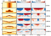 |
Fig. 1 Time evolution of the non-magnetic model. The top row shows the initial snapshot, with subsequent time snapshots taken every 20 ks. The left column shows the temperature in kelvins, the middle column shows the horizontal flow velocity, and the right column shows the vertical flow velocity in cm s−1. Red colour in the middle panel represents lateral motion of the gas to the right and blue represents motion to the left. Likewise, the red colour in the right panel represents upward flow while blue represents downward motion. |
3.2 Standard 10 G horizontal magnetic model
Fig. 2 illustrates the time evolution of our standard magnetic model, which includes a 10 G uniform horizontal magnetic field. In this model, the horizontal magnetic field is sufficiently strong to suppress vertical flows, which significantly reduces the vertical mixing of gas. However, the magnetic field strength is not high enough to impede horizontal flows, allowing hot gas to spread laterally with speeds of around 104 cm s−1. Consequently, while a vertical temperature gradient is maintained, the hot gas is able to diffuse horizontally away from the initial chemical spot, which leads to a more uniform temperature distribution across the stellar surface.
This behaviour contrasts with cases involving stronger magnetic fields (see Table 1), where both vertical and horizontal flows are heavily suppressed. In such cases of strong magnetic fields, the temperature stratification remains tightly confined to the chemical spot region due to the strong magnetic inhibition of flow. By comparing these cases, we gain insight into how varying magnetic field strengths influence the transport of energy and matter within the atmosphere, with intermediate fields allowing lateral diffusion and stronger fields creating isolated, thermally stratified regions.
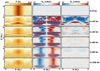 |
Fig. 2 Time evolution of the standard magnetic model with an initial uniform 10 G magnetic field (black lines) in the horizontal direction. The top row shows the initial time snapshot, with subsequent time snap-shots taken every 20 ks. The left column shows the temperature in kelvins, the middle column shows the horizontal flow velocity, and the right column shows the vertical flow velocity in cm s−1. Note that the range for velocity is a factor of 10 lower than for the non-magnetic case in Fig. 1. This highlights the effects the magnetic field can have on atmospheric flow. |
3.3 Parameter study
To help us assess the general effects of magnetic fields on atmospheric dynamics, Fig. 3 displays the horizontal flow velocities across all models at the conclusion of our simulations. The left column shows cases with a uniform vertical magnetic field orientation, while the right column shows those with a horizontal magnetic field. The results indicate a clear trend: a strong vertical magnetic field effectively suppresses horizontal flows by stabilizing the atmosphere against lateral motion. In our setup, the magnetic field energy density overcomes the gas energy density from as early as the 1 G magnetic field at the top of the photosphere. Therefore, the horizontal flow can be suppressed by a vertical field with a strength of 1 G. In contrast, models with strong horizontal magnetic fields produce a gentle, steady horizontal flow or ‘breeze’, of approximately 104 cm s−1. This horizontal flow may play an important role in diffusing and eroding surface abundance spots, thereby reducing their lifetime.
The pattern for vertical flow velocities, shown in Fig. 4, reveals nearly the opposite behaviour. Vertical magnetic fields inhibit horizontal flows but allow for limited vertical motion. However, given that the primary temperature gradient in our simulations is oriented horizontally, the absence of sufficient horizontal flow inhibits the effective mixing of hot and cool gas, thereby limiting the formation of strong vertical flows.
This dynamics is further emphasized in Fig. 5, which shows the final temperature distribution for each model. In nonmagnetic and weakly magnetized cases (1 and 10 G), horizontal flows facilitate the mixing of hot and cool gas, which leads to a more homogenized temperature distribution. In contrast, in models with strong magnetic fields, the initial temperature stratification is largely preserved. Here, the magnetic field prevents substantial lateral mixing, which maintains localized regions of hot and cool gas near the initial configuration (Peterson 1970).
These findings underscore the influence of the magnetic field orientation and strength on atmospheric dynamics. Strong vertical fields stabilize the atmosphere laterally, while strong horizontal fields promote diffusion. This magnetic regulation of flow has implications for the persistence and evolution of surface abundance features, particularly in magnetic chemically peculiar stars where such abundance anomalies are often observed.
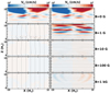 |
Fig. 3 Horizontal flow velocity for vertical (left column) and horizontal (right column) magnetic field configurations for all the models shown at the final time, t = 100 ks, with the exception of the non-magnetic case (top row) shown at time t = 80 ks, which is coincidentally more representative than the final time snapshot. The magnetic field strength increases from the top to the bottom. |
4 Discussion
Our simulations were calculated for a specific set of stellar parameters corresponding to a particular helium-strong chemically peculiar star. However, the phenomenon studied in this paper is not limited to this specific set of parameters, but is applicable to all stars with an inhomogeneous surface abundance distribution, albeit with differing strengths and timescales. The interplay between radiative diffusion, horizontal flows, and other processes that influence abundance evolution suggests that the underlying mechanisms operate across various stellar types, even though the specific characteristics and evolutionary timescales of abundance inhomogeneities can vary significantly.
In non-magnetic stars of spectral type BA, our simulations presented here estimate the speed of the atmospheric flow connected to horizontal temperature inhomogeneities to be of the order of 105 cm s−1 (cf. Sect. 3.1). Taking into account the typical radius of such a star, the mixing timescale is of the order of tens of days. However, it is conceivable that normal BA stars possess surface magnetic fields with typical strengths of the order of 1 G (Lignières et al. 2009; Petit et al. 2011; Blazère et al. 2020). In such a case, the typical flow velocities become an order of magnitude lower (cf. Sect. 3.2), which leads to typical flow timescales of the order of years. This corresponds to a typical timescale of the evolution of surface abundance spots in HgMn stars (Briquet et al. 2010; Korhonen et al. 2013), thus highlighting a generally good agreement between our model and observations.
In general, the timescale of the spot evolution is comparable with the radiative diffusion timescale. However, this timescale strongly depends on the location in the atmosphere and on the properties of a particular element, such as the local relative abundance. Consequently, the radiative diffusion timescale can be as short as days in the upper parts of the atmosphere, while it might take centuries in deep photospheric layers (Alecian et al. 2011). For the specific case of mercury in the continuum-forming photospheric regions, the radiative diffusion timescale is comparable to the year timescales of horizontal flows. This implies that the photospheric flows and radiative diffusion operate on similar timescales in HgMn stars; therefore, horizontal flow could be one of the processes that precludes strong abundance anomalies in stars with weak magnetic fields. Although such flows may contribute to the dynamical evolution of abundance spots, we caution that the timescale to build the peculiar abundances could be longer.
This suggests that while the radiative diffusion timescale may be relatively short in certain regions, the actual process of creating abundance inhomogeneities involves additional factors that extend the overall timescale. These factors include complex interactions between photospheric flows and radiative diffusion, as well as the slower processes of element migration and accumulation. As a result, the timescale for the creation of abundance inhomogeneities might be longer than the radiative diffusion timescale alone would suggest. Understanding these extended timescales is crucial for accurately modelling and interpreting the abundance patterns observed in HgMn stars.
For the mass-loss rates predicted in the magnetic helium-strong star HD 37776 (Krtička 2014), the wind velocity in the continuum-forming regions of the photosphere, which is of the order of 10 cm s−1, is lower than the velocity of the horizontal flows. However, the stellar wind quickly accelerates and overcomes the horizontal flow velocity by one to two orders of magnitude in the upper parts of the photosphere.
On the other hand, our simulations show that magnetic fields stronger than about 100 G inhibit any flow generated by the horizontal temperature gradients. These are the typical fields that are detected in magnetic chemically peculiar stars (Morel et al. 2015; Wade et al. 2016; Grunhut et al. 2017). Therefore, inhibition of the horizontal flow by the vertical magnetic field contributes to the establishment of abundance anomalies and their stability. Nevertheless, even in these stars, relatively rapid flows with speeds of the order of 103 cm s−1 are possible in those regions with horizontal magnetic fields. Such flows can contribute to the stratification of chemical elements in magnetic chemically peculiar stars.
The atmospheric flows induced by horizontal temperature gradients may reach up to 105 cm s−1. In principle, such velocities could just about be detected using Doppler imaging. Future observational campaigns might help us verify the predictions of our simulations.
5 Summary and future work
Our study investigated the effects of magnetic fields on the atmospheric dynamics of chemically peculiar stars, focusing on how different magnetic field strengths and orientations influence horizontal and vertical flows. Photospheric flows supposedly originate from horizontal temperature inhomogeneities connected with abundance stratification. We find that strong vertical magnetic fields inhibit horizontal flows, and thus preserve temperature stratification and stabilize abundance anomalies. Conversely, strong horizontal magnetic fields enable a lateral ‘breeze’, which can erode surface abundance spots over time. In weak or non-magnetic cases, the horizontal flow effectively mixes hot and cool gas, resulting in a more homogenized temperature distribution.
Our results for a flow velocity of around 104 cm s−1, which leads to flux timescales of the order of a year, are in good agreement with the typical timescale for the evolution of surface abundance spots in HgMn stars obtained from observations. Our simulations also confirm that a weak horizontal flow can contribute to the dynamical evolution of abundance spots in HgMn stars. On the other hand, a strong vertical magnetic field (~100 G) can inhibit the horizontal flow and initiate the formation and stabilization of abundance anomalies in chemically peculiar stars.
Future work should expand these simulations to full three dimensions to capture the complete complexity of flow dynamics and magnetic interactions in stellar atmospheres of chemically peculiar stars. More realistic simulations also require a more detailed treatment of energy equations that account for the radiative equilibrium. Additionally, relaxing the planar atmosphere assumption and incorporating a more realistic, curved stellar surface will allow us to more accurately model atmospheric flows and temperature distributions. These improvements will provide deeper insights into the evolution of surface abundance features in magnetic chemically peculiar stars.
Acknowledgements
A.u.-D. acknowledges NASA ATP grant number 80NSSC22K0628 and support by NASA through Chandra Award number TM4-25001A issued by the Chandra X-ray Observatory 27 Center, which is operated by the Smithsonian Astrophysical Observatory for and on behalf of NASA under contract NAS8-03060. The Astronomical Institute of the Czech Academy of Sciences in Ondřejov is supported by the project RVO:67985815. B.K. acknowledges the support from the Grant Agency of the Czech Republic (GAĈR 22-34467S).
References
- Alecian, G., & Stift, M. J. 2017, MNRAS, 468, 1023 [Google Scholar]
- Alecian, G., & Stift, M. J. 2019, MNRAS, 482, 4519 [Google Scholar]
- Alecian, G., Stift, M. J., & Dorfi, E. A. 2011, MNRAS, 418, 986 [NASA ADS] [CrossRef] [Google Scholar]
- Blazère, A., Petit, P., Neiner, C., et al. 2020, MNRAS, 492, 5794 [CrossRef] [Google Scholar]
- Briquet, M., Korhonen, H., González, J. F., Hubrig, S., & Hackman, T. 2010, A&A, 511, A71 [NASA ADS] [CrossRef] [EDP Sciences] [Google Scholar]
- Catanzaro, G., Giarrusso, M., Leone, F., et al. 2016, MNRAS, 460, 1999 [NASA ADS] [CrossRef] [Google Scholar]
- Das, B., Chandra, P., Shultz, M. E., et al. 2022, ApJ, 925, 125 [NASA ADS] [CrossRef] [Google Scholar]
- Faltová, N., Kallová, K., Prišegen, M., et al. 2021, A&A, 656, A125 [NASA ADS] [CrossRef] [EDP Sciences] [Google Scholar]
- Fuller, J., & Mathis, S. 2023, MNRAS, 520, 5573 [CrossRef] [Google Scholar]
- Grunhut, J. H., Wade, G. A., Neiner, C., et al. 2017, MNRAS, 465, 2432 [NASA ADS] [CrossRef] [Google Scholar]
- Hayes, J. C., Norman, M. L., Fiedler, R. A., et al. 2006, ApJS, 165, 188 [NASA ADS] [CrossRef] [Google Scholar]
- Hümmerich, S., Mikulášek, Z., Paunzen, E., et al. 2018, A&A, 619, A98 [NASA ADS] [CrossRef] [EDP Sciences] [Google Scholar]
- Jagelka, M., Mikulášek, Z., Hümmerich, S., & Paunzen, E. 2019, A&A, 622, A199 [NASA ADS] [CrossRef] [EDP Sciences] [Google Scholar]
- Khan, S. A., & Shulyak, D. V. 2007, A&A, 469, 1083 [NASA ADS] [CrossRef] [EDP Sciences] [Google Scholar]
- Kochukhov, O., & Ryabchikova, T. A. 2018, MNRAS, 474, 2787 [NASA ADS] [CrossRef] [Google Scholar]
- Kochukhov, O., & Wade, G. A. 2010, A&A, 513, A13 [NASA ADS] [CrossRef] [EDP Sciences] [Google Scholar]
- Kochukhov, O., Lundin, A., Romanyuk, I., & Kudryavtsev, D. 2011, ApJ, 726, 24 [NASA ADS] [CrossRef] [Google Scholar]
- Kochukhov, O., Makaganiuk, V., Piskunov, N., et al. 2013, A&A, 554, A61 [NASA ADS] [CrossRef] [EDP Sciences] [Google Scholar]
- Kochukhov, O., Khalack, V., Kobzar, O., et al. 2021, MNRAS, 506, 5328 [NASA ADS] [CrossRef] [Google Scholar]
- Korhonen, H., González, J. F., Briquet, M., et al. 2013, A&A, 553, A27 [NASA ADS] [CrossRef] [EDP Sciences] [Google Scholar]
- Krtička, J. 2014, A&A, 564, A70 [NASA ADS] [CrossRef] [EDP Sciences] [Google Scholar]
- Krtička, J., Mikulášek, Z., Zverko, J., & Žižn?ovský, J. 2007, A&A, 470, 1089 [NASA ADS] [CrossRef] [EDP Sciences] [Google Scholar]
- Krtička, J., Mikulášek, Z., Lüftinger, T., et al. 2012, A&A, 537, A14 [NASA ADS] [CrossRef] [EDP Sciences] [Google Scholar]
- Krtička, J., Mikulášek, Z., Lüftinger, T., & Jagelka, M. 2015, A&A, 576, A82 [NASA ADS] [CrossRef] [EDP Sciences] [Google Scholar]
- Krtička, J., Mikulášek, Z., Prvák, M., et al. 2020, MNRAS, 493, 2140 [Google Scholar]
- Labadie-Bartz, J., Hümmerich, S., Bernhard, K., Paunzen, E., & Shultz, M. E. 2023, A&A, 676, A55 [NASA ADS] [CrossRef] [EDP Sciences] [Google Scholar]
- Leto, P., Trigilio, C., Krticka, J., et al. 2021, MNRAS, 507, 1979 [NASA ADS] [CrossRef] [Google Scholar]
- Lignières, F., Petit, P., Böhm, T., & Aurière, M. 2009, A&A, 500, L41 [CrossRef] [EDP Sciences] [Google Scholar]
- Makaganiuk, V., Kochukhov, O., Piskunov, N., et al. 2012, A&A, 539, A142 [NASA ADS] [CrossRef] [EDP Sciences] [Google Scholar]
- Michaud, G., Tarasick, D., Charland, Y., & Pelletier, C. 1983, ApJ, 269, 239 [Google Scholar]
- Michaud, G., Richer, J., & Vick, M. 2011, A&A, 534, A18 [NASA ADS] [CrossRef] [EDP Sciences] [Google Scholar]
- Michaud, G., Alecian, G., & Richer, J. 2015, Atomic Diffusion in Stars, Astronomy and Astrophysics Library (Springer International Publishing Switzerland) [CrossRef] [Google Scholar]
- Mikulášek, Z., Krticka, J., Henry, G. W., et al. 2008, A&A, 485, 585 [NASA ADS] [CrossRef] [EDP Sciences] [Google Scholar]
- Molnar, M. R. 1973, ApJ, 179, 527 [NASA ADS] [CrossRef] [Google Scholar]
- Morel, T., Castro, N., Fossati, L., et al. 2015, in New Windows on Massive Stars, eds. G. Meynet, C. Georgy, J. Groh, & P. Stee, IAU Symposium, 307, 342 [Google Scholar]
- Owocki, S. P., Shultz, M. E., ud-Doula, A., et al. 2022, MNRAS, 513, 1449 [NASA ADS] [CrossRef] [Google Scholar]
- Peterson, D. M. 1970, ApJ, 161, 685 [NASA ADS] [CrossRef] [Google Scholar]
- Petit, P., Lignières, F., Aurière, M., et al. 2011, A&A, 532, L13 [NASA ADS] [CrossRef] [EDP Sciences] [Google Scholar]
- Potravnov, I., Piskunov, N., & Ryabchikova, T. 2024, A&A, 689, A111 [NASA ADS] [CrossRef] [EDP Sciences] [Google Scholar]
- Prvák, M., Liška, J., Krticka, J., Mikulášek, Z., & Lüftinger, T. 2015, A&A, 584, A17 [NASA ADS] [CrossRef] [EDP Sciences] [Google Scholar]
- Prvák, M., Krticka, J., & Korhonen, H. 2020, MNRAS, 492, 1834 [CrossRef] [Google Scholar]
- Ryabchikova, T., Kochukhov, O., & Bagnulo, S. 2008, A&A, 480, 811 [NASA ADS] [CrossRef] [EDP Sciences] [Google Scholar]
- Wade, G. A., Neiner, C., Alecian, E., et al. 2016, MNRAS, 456, 2 [Google Scholar]
All Tables
All Figures
|
Fig. 1 Time evolution of the non-magnetic model. The top row shows the initial snapshot, with subsequent time snapshots taken every 20 ks. The left column shows the temperature in kelvins, the middle column shows the horizontal flow velocity, and the right column shows the vertical flow velocity in cm s−1. Red colour in the middle panel represents lateral motion of the gas to the right and blue represents motion to the left. Likewise, the red colour in the right panel represents upward flow while blue represents downward motion. |
| In the text | |
|
Fig. 2 Time evolution of the standard magnetic model with an initial uniform 10 G magnetic field (black lines) in the horizontal direction. The top row shows the initial time snapshot, with subsequent time snap-shots taken every 20 ks. The left column shows the temperature in kelvins, the middle column shows the horizontal flow velocity, and the right column shows the vertical flow velocity in cm s−1. Note that the range for velocity is a factor of 10 lower than for the non-magnetic case in Fig. 1. This highlights the effects the magnetic field can have on atmospheric flow. |
| In the text | |
|
Fig. 3 Horizontal flow velocity for vertical (left column) and horizontal (right column) magnetic field configurations for all the models shown at the final time, t = 100 ks, with the exception of the non-magnetic case (top row) shown at time t = 80 ks, which is coincidentally more representative than the final time snapshot. The magnetic field strength increases from the top to the bottom. |
| In the text | |
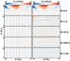 |
Fig. 4 Same as Fig. 3 but for vertical flow velocity. |
| In the text | |
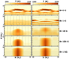 |
Fig. 5 Same as Fig. 3 but for temperature. |
| In the text | |
Current usage metrics show cumulative count of Article Views (full-text article views including HTML views, PDF and ePub downloads, according to the available data) and Abstracts Views on Vision4Press platform.
Data correspond to usage on the plateform after 2015. The current usage metrics is available 48-96 hours after online publication and is updated daily on week days.
Initial download of the metrics may take a while.