| Issue |
A&A
Volume 639, July 2020
|
|
|---|---|---|
| Article Number | A27 | |
| Number of page(s) | 14 | |
| Section | Extragalactic astronomy | |
| DOI | https://doi.org/10.1051/0004-6361/202037555 | |
| Published online | 03 July 2020 | |
Radio emission during the formation of stellar clusters in M 33
1
INAF-Osservatorio Astrofisico di Arcetri, Largo E. Fermi, 5, 50125 Firenze, Italy
e-mail: This email address is being protected from spambots. You need JavaScript enabled to view it.
2
Laboratoire d’Astrophysique de Bordeaux, Univ. Bordeaux, CNRS, B18N, allée Geoffroy Saint-Hilaire, 33615 Pessac, France
3
School of Astronomy, Institute for Research in Fundamental Sciences, PO Box 19395-5531, Tehran, Iran
4
Instituto de Astrofísica de Canarias, 38205 San Cristóbal de La Laguna, Tenerife, Spain
5
Max-Planck-Institut für Astronomie, Königstuhl 17, 69117 Heidelberg, Germany
Received:
22
January
2020
Accepted:
5
May
2020
Abstract
Aims. We investigate thermal and nonthermal radio emission associated with the early formation and evolution phases of young stellar clusters (YSCs) selected by their mid-infrared (MIR) emission at 24 μm in M 33. We consider regions in their early formation period, which are compact and totally embedded in the molecular cloud, and in the more evolved and exposed phase.
Methods. Thanks to recent radio continuum surveys between 1.4 and 6.3 GHz we are able to find radio source counterparts to more than 300 star forming regions of M 33. We identify the thermal free–free component for YSCs and their associated molecular complexes using the Hα line emission.
Results. A cross-correlation of MIR and radio continuum is established from bright to very faint sources, with the MIR-to-radio emission ratio that shows a slow radial decline throughout the M 33 disk. We confirm the nature of candidate embedded sources by recovering the associated faint radio continuum luminosities. By selecting exposed YSCs with reliable Hα flux, we establish and discuss the tight relation between Hα and the total radio continuum at 5 GHz over four orders of magnitude. This holds for individual YSCs as well as for the giant molecular clouds hosting them, and allows us to calibrate the radio continuum–star formation rate relation at small scales. On average, about half of the radio emission at 5 GHz in YSCs is nonthermal with large scatter. For exposed but compact YSCs and their molecular clouds, the nonthermal radio continuum fraction increases with source brightness, while for large HII regions the nonthermal fraction is lower and shows no clear trend. This has been found for YSCs with and without identified supernova remnants and underlines the possible role of massive stars in triggering particle acceleration through winds and shocks: these particles diffuse throughout the native molecular cloud prior to cloud dispersal.
Key words: radio continuum: galaxies / galaxies: star formation / galaxies: groups: individual: M 33 / dust / extinction / ISM: molecules / galaxies: star clusters: general
© ESO 2020
1. Introduction
The radio continuum–infrared (IR) correlation in galaxies was first investigated following the data release by IRAS mission (e.g., Helou et al. 1985; Bell 2003). In the past 35 years, a lot of effort has been made to investigate the frequency ranges in the IR and radio continuum for which the correlation is the tightest and how these depend on spatial scale. In the IR domain, the focus has been to distinguish warm dust emitting in the mid-infrared (MIR) and heated by star formation from cold dust heated by the interstellar radiation field and emitting in the far-infrared. In the radio continuum, both thermal (free-free) and nonthermal (synchrotron) emission are linked to the formation of stars since this process is responsible for the free electrons, as well as for turbulent magnetic field amplification and cosmic ray (CR) production (e.g., Schleicher & Beck 2013; Schober et al. 2016; Tabatabaei et al. 2013a). A key question is the spatial scale involved in the dust-to-radio correlation, and to this purpose nearby galaxies such as LMC, M 33, M51 and so on have been analyzed using wavelet decomposition and maps at several spatial resolutions, from 50 pc out to the kiloparsec scales, for the radio and IR emission (Hughes et al. 2006; Tabatabaei et al. 2007a, 2013b; Dumas et al. 2011). On large scales, the ordered magnetic field seems to play a major role in driving nonthermal emission, especially where cosmic rays are able to diffuse away from star forming sites before losing their energy. Therefore, the magnetic field might be coupled to cold dust by density enhancement in the diffuse interstellar medium (ISM; Basu et al. 2017). Dumas et al. (2011) explored how the relation between the MIR and radio continuum in M51 depends on the local environment, such as spiral arms, interarm regions, and outer versus inner disk, and found that a linear relation holds only along the spiral arms with radio synchrotron emission being suppressed in the central regions.
On small scales, it is interesting to study the nonthermal and thermal component and how these relate to the warm dust as a function of the ISM properties and environment in the galactic disk. Data in the radio continuum at 1.4 GHz and in the IR at 60 μm have been analyzed by Hughes et al. (2006) for the LMC at spatial scales between 50 pc and 1.5 kpc. On small scales the thermal radio emission correlates better with the warm dust component while the nonthermal far-infrared correlation breaks down below a certain scale possibly because of the large diffusion length of cosmic rays. More recently, a study of IC10 by Basu et al. (2017) showed that also at smaller scales, between 50 and 200 pc, the nonthermal radio emission establishes a better correlation with the dust emission at 70 μm than with the warm dust at 24 μm. However there are no studies analyzing individual star forming regions where the 24 μm emission peaks.
The large-scale magnetic field in M 33 exhibits a spiral structure with a decrease in the radio thermal fraction going radially outwards (Tabatabaei et al. 2007b). At kiloparsec scales in M 33, the warm dust–thermal radio correlation is stronger than the cold dust–nonthermal radio correlation (Tabatabaei et al. 2007a), although a cold dust–nonthermal correlation still holds. An analysis of the radio emission in the closest spiral galaxies (Tabatabaei et al. 2013b) showed that the nonthermal–IR correlation is weaker in M 33 than in M31 on large scales, but that the opposite is true on scales < 1 kpc. This has been explained by the smaller propagation length of CR electrons in M 33 due to its turbulent magnetic field structure. At smaller scales, the turbulent magnetic field might become more important as turbulent gas motion injects energy into the ISM (Tabatabaei et al. 2008). If this is a general property of the ISM of M 33, the nonthermal–IR correlation should also hold on scales where the turbulent magnetic field is strongest, such as in the star forming clouds.
For nearby galaxies, the sensitivity and spatial resolution of IR and radio surveys is now sufficiently high that it is possible to isolate individual star forming regions with stellar masses as low as a few hundred solar masses (Sharma et al. 2011; White et al. 2019). This means that instead of focusing on the spatial scale and on a pixel-by-pixel analysis, one can examine the radio and IR emission in individual star forming regions and how this depends on characteristic properties of the young cluster such as mass and age and, more generally, on the energy input that massive stars can provide. In the present paper we analyze the radio continuum and MIR emission in individual star forming sites of M 33, the closest blue spiral galaxy. This allows us to test whether the correlation between the nonthermal radio and MIR emission found down to 200 pc scale (Tabatabaei et al. 2013b) also holds at smaller scales for the emission of individual young stellar clusters (YSCs). Previous works have presented a catalog of IR-selected star forming regions across the whole disk of M 33 (Sharma et al. 2011) which has been complemented by a catalog of giant molecular clouds (GMCs; Corbelli et al. 2017). Furthermore, a list of radio-continuum sources in the M 33 area recently became available (White et al. 2019), some of which might be related to the M 33 disk. The spatial resolution at 24 μm is comparable to that of the recent radio-continuum surveys. Our aim is to investigate the correlations between the radio continuum and other star formation tracers such as Hα or MIR emission and investigate the dominant mechanism that provides radio emission, thermal or nonthermal, across a variety of star forming regions. While it is clear that the turbulent magnetic field is enhanced in star forming regions, it is less clear how this depends on the characteristics of the region and its location in the disk. Furthermore, the creation and propagation of CRs might depend on the galaxy (Tabatabaei et al. 2013b) and on characteristics of the star forming region.
Currently, most of the models involving CR acceleration are based on supernova explosions and their remnants. In particular, these models can explain the CR production rate, composition, and anisotropy in our Galaxy. However, the steepness and the presence of breaks in supernova spectra, as well as the difficulties in explaining the very energetic CRs, suggest that other types of acceleration mechanisms may exist. Moreover, the duration of the supernova shock might be too short to explain the propagation away from the remnants that is needed to explain some observations. Over the last decade, space- and ground-based telescopes have revealed many classes of Galactic γ-ray sources, such as clusters of young stars, which might be associated to CR accelerators. As underlined recently by Aharonian et al. (2019), the acceleration could take place in the vicinity of the stars or in superbubbles, caused by interacting winds of massive stars such as those in OB associations. A fraction of the mechanical energy in stellar wind may be transferred to relativistic CRs by diffuse shock acceleration at the wind boundary (Cesarsky & Montmerle 1983; Parizot et al. 2004; Padovani et al. 2019). These CRs could then spiral around the fluctuating amplified magnetic fields of the star forming region emitting nonthermal radio waves. To test these possibilities, recently identified supernova remnants (SNRs) in star forming regions of M 33 (White et al. 2019) can be used to assess the role of massive stars and stellar winds in enhancing the nonthermal radio emission in star forming regions.
The present paper is organized as follows: in Sect. 2 we present the data and the method used to establish the association between MIR and radio sources. In Sect. 3 we present the correlation between radio continuum and MIR fluxes in exposed YSCs and in the embedded star forming sites in M 33. In Sect. 4 we derive the nonthermal fractions and the relative implications. In Sect. 5 we present some preliminary results on radio emission from GMCs, and in Sect. 6 we discuss the link between star formation and radio continuum. Section 7 summarizes the main results of our analysis.
2. The YSC sample and multiwavelength data
In this section we describe how we select candidate YSCs in M 33 during their formation and early evolutionary phases and how we retrieve the emission at other wavelengths. We use three catalogs now available for M 33: a 24 μm source catalog (Sharma et al. 2011), a GMC catalog (Corbelli et al. 2017) and a radio continuum source catalog (White et al. 2019). The association is done by matching the positions in the sky of the objects in these catalogs because the shape and extend of the emission of a star forming region in the MIR and in the radio continuum might not be the same. The hot dust for example might be located closer to the GMC center or to the shell of an expanding ionized bubble while nonthermal radio continuum emission might peak close to a SNR. In the following analysis of M 33, we assume a distance of 840 kpc (Freedman et al. 1991; Gieren et al. 2013).
2.1. The MIR source catalog
Dust emission at MIR wavelengths has been investigated through data of the Multiband Imaging Photometer (MIPS) on the Spitzer Space Telescope processed as described by Verley et al. (2007). Corbelli et al. (2017) selected 630 MIR sources from the list of Sharma et al. (2011) that are candidate YSCs in the early formation and evolutionary phases: the results of the classification, together with the most relevant parameters of the GMCs and YSCs, can be found in their online tables. The YSCs were sorted into classes based on their emission in the MIR, far ultraviolet (FUV), and Hα bands and according to the association with GMCs. The classification helps in drawing a possible evolutionary sequence and the relative timescales see Corbelli et al. (2017) for more details. We recall the classification scheme of the MIR sources and the number of MIR sources in each category:
-
Class b: 97 MIR sources, associated with GMCs, with no optical counterpart (with no or very weak Hα peak);
-
Class c: 410 YSCs with optical counterpart
-
c1: 55 YSCs associated with GMCs with coincident Hα and MIR emission peaks but FUV emission spatially shifted or absent;
-
c2: 218 YSCs associated with GMCs with coincident Hα, FUV and MIR emission peaks;
-
c3: 139 YSCs not associated with GMCs but with optical and FUV counterparts; these often have weak Hα emission;
-
-
Class d: 19 MIR sources associated with GMCs which are ambiguous for b or c1/c2 class;
-
Class e: 104 MIR sources not associated with GMCs and with no Hα emission, some FUV may be present.
The b-c1-c2-d-type are sources associated with GMCs. The b-type are called embedded because there is no FUV or Hα counterparts, while c-type are exposed star forming regions with FUV and Hα counterpart and some of them (c1 and c2) are associated with GMC while others (c3) are not. The d-type are ambiguous between b-and c-type. From now on we shall refer to the c-class as exposed YSCs and to the b-type as embedded YSCs. Extinction is high for b-type sources with weak or no FUV or optical counterpart, which likely represent the early phases of star formation. The c1-type YSCs have visible Hα but not FUV emission and show on average higher extinction than the c2-type YSCs, where FUV emission is also detected. The c1-type YSCs may represent YSCs at an earlier stage than c2-type YSCs, even though the YSC age determination is not precise enough to separate these two classes. The most luminous MIR sources are of c2-type and are clusters that have very likely completed the formation process. This is also the largest class of MIR sources for which the coincident peaks in the FUV and Hα bands enabled more precise estimates of the age and mass of the associated YSC.
The e-type sources have only MIR emission but unlike the b-type these do not have any associated GMC. We marginally consider the e-type in this paper. As shown in subsequent sections and also in the paper by Corbelli et al. (2019) where deep CO searches have been carried out, the e-type are highly contaminated by background sources and thus most of them do not belong to M 33. Background contamination is particularly relevant for dim sources, with flux at 24 μm smaller than 5 mJy, and no associated molecular cloud or Hα emission such as type-e sources Corbelli et al. (2019). We cannot exclude, however that a few of them might be embedded YSCs in low mass molecular clouds.
2.2. The molecular cloud catalog
Using the IRAM 30m CO J = 2 − 1 data cube of M 33, we identified 566 GMCs, as described in Corbelli et al. (2017), and whose properties are listed in the GMCs catalog. The GMC masses are between 2 × 10⁴ and 2 × 10⁶ M⊙ and GMC radii between 10 and 100 pc The number of GMCs above the survey completeness limit (MH2 ≥ 6.3 × 10⁴ M⊙) is 490. Corbelli et al. (2017) classified the GMCs as non-starforming (class A), with embedded star formation (B), or with exposed star formation (C). A few ambiguous cases are in class D. The FUV, Hα and MIR emission maps of M 33 have been used to classify the GMCs.
The majority of the MIR sources in the inner zones (R< 4 kpc) lie within a GMC boundary while this is not true for MIR sources in the outer disk. There is an extraordinary spatial correspondence between the GMCs and the distribution of atomic hydrogen overdensities in the inner zones. In the outer zone there are fewer GMCs, possibly because of a steepening of the molecular cloud mass spectrum, with a larger fraction of clouds being below the survey completeness limit.
2.3. The radio source catalog
Recently using Karl Jansky Very Large Array (JVLA) radio continuum maps of M 33 at 1.4 and 5 GHz at a spatial resolution of about 6 arcsec, White et al. (2019) catalogd 2875 sources with fluxes between 2 and 33 000 μJy (except for one with a flux of about 0.17 Jy) with a completeness limit around 300 μJy. Most of the luminous radio sources are stellar-like objects, background QSOs or MW stars; a few are sources associated with the two most prominent HII regions of M 33, NGC 604 and NGC 595, which we exclude from the current analysis because of their extended and complex structure. White et al. (2019) have also identified SNR using the optical catalogs of Long et al. (2010), Lee & Lee (2014). Background contamination is present at all flux densities in radio but the number of background sources dominates over local sources in number as the flux gets below 300 μJy. To identify M 33 sources it is therefore mandatory to use identification of other counterparts with line emission such as Hα and molecular clouds.
2.4. Emission at other wavelengths
For MIR sources we have recovered the emission at other wavelengths, such as Hα, by aperture photometry which has been described in detail by Sharma et al. (2011). We noticed that the for radio sources coincident with MIR sources the Hα emission in White et al. (2019) catalog was much lower that that associated to MIR sources by Sharma et al. (2011), especially for bright sources. Accurate Hα photometry is needed to estimate the thermal fraction of radio emission from YSCs. Therefore to trace the ionized gas associated to radio sources we perform new aperture photometry, centering a circular aperture on radio source coordinates. We set the aperture radius equal to 1.5 times the mean between the semiminor and semimajor source axis, and subtracting the local background (see Sharma et al. 2011, for more details on aperture photometry). As described by Hoopes & Walterbos (2000) M 33 has, in fact, a non negligible diffuse fraction of ionized gas due to leakage of ionizing photons from HII regions and to massive stars in the field. An aperture larger than the source radius account for the position of the source center and extension which may change with wavelength. We adopt the narrow-line Hα image of M 33 obtained by Greenawalt (1998) and described in detail in Hoopes & Walterbos (2000). As suggested by the authors a 5% contamination by NII has been considered and accounted for.
Additional radio observations of M 33 were carried out with the JVLA at C-band (5.5–7.5 GHz) in D configuration as part of the Cloud-scale Radio Survey of Star Formation and Feedback In Triangulum galaxy (CRASSFIT, Tabatabaei et al., in prep.) between November 2011 and March 2012. Two continuous base-bands (of 1024 MHz) were tuned at 5.5–6.5 GHz and 6.5–7.5 GHz, each with 8 sub-bands of 128 MHz. A mosaic of 5 × 5 was used to cover the inner 18′×18′ star forming region including the main spiral arms with similar sensitivity. The total on-source observing time per pointing was about one hour leading to an rms noise of 6 μJ per  beam in the final image. The two sources 3C 48 and 3C 138 were used as the primary flux density and the antenna gain phase calibrator during the observations. The data were reduced in the Obit package (Cotton 2008) using the standard VLA calibration procedure. Each pointing was imaged and then combined into a mosaic using the wideband Obit imager MFImage (Cotton et al. 2018). We shall refer to this dataset as the 6.3 GHz map. The negative sidelobes sometime visible in the White et al. (2019) maps are not present in the 6.3 GHz map which can be used for deeper and more sensitive searches of YSCs radio counterparts.
In performing aperture photometry for radio sources on the 6.3 GHz map we use circular apertures with aperture radius equal to the source radius at 1.4 GHz convolved with the beam of the 6.3 GHz map. We subtract the local background, having corrected the 6.3 GHz map for missing short spacing, using the “mode” function in a 3 pixel wide annulus at a distance of at least 4 pixels from source aperture boundary.
We would like to underline here that we have also performed aperture photometry without background subtraction both on Hα and on radio continuum maps. The results discussed in the next Sections remain unchanged since flux variations are marginal with the largest flux increase being that relative to the 6.3 GHz data. In Sect. 4, where we separate the thermal and nonthermal radio flux at 5 GHz using Hα emission, we also show results for a varying aperture size and using a smoothed version of the Hα image. This has been obtained by convolving the original map (at about 3 arcsec spatial resolution) with a gaussian function of 6 arcsec FWHM, which is the spatial resolution of the 24 μm and 5 GHz maps.
Photometry for emission within GMCs is carried out using the irregular GMC shape recovered by Corbelli et al. (2017). The shapes and GMC images are available for a subsample of them in the online version of Gratier et al. (2012). No background is subtracted in this case although some low level of diffuse emission might be associated with the atomic gas in the M 33 disk along the line of sigh to the GMC.
2.5. Uncertainties
The 1.4 GHz map of White et al. (2019) is less affected by sidelobes than the 5 GHz map and we trust the sources identified in the catalog at 1.4 GHz. The source flux at 5 GHz can be recovered using the cataloged spectral indexes and flux at 1.4 GHz. This is in good agreement with the flux recovered at 6.3 GHz if we use the 6.3 GHz map before corrections for short spacing are applied. As noticed by White et al. (2019), source fluxes at 1.4 GHz are lower than those of Gordon et al. (1999) and to get an agreement a positive correction is needed. Increasing the 1.4 GHz fluxes of White et al. (2019) by about 30% brings them in agreement with the fluxes recovered using the 1.4 GHz map of Tabatabaei et al. (2007b) and the unpublished JVLA map at the same frequency (Tabatabaei et al., in prep.). Moreover, in the radio catalog the HII region spectral indices are mostly positive, with a mean value of about 0.1, while we expect them to be negative because optically thick radio emission on the scale of tens of parsecs is unlikely. Increasing the 1.4 GHz fluxes by 30% implies spectral indices lower by about 0.2 and hence more physically reasonable. However, in this paper we use the 1.4 GHz data without applying any correction but we shall focus more on the high frequency emission at 5 and 6.3 GHz, for which no calibration corrections are needed. We use the White et al. (2019) data considering 30% calibration errors in addition to photometric and spectral index uncertainties.
Photometric errors for Hα are negligible and calibration errors are of order 5%.
3. Radio sources in star forming regions
To have an overview of the radio sources in the M 33 area we plot in Fig. 1 the radio flux at 1.4 GHz for all sources in the White et al. (2019) catalog versus Hα emission given in the same catalog. There are clearly two distinct source populations, one for which the radio and Hα flux establish a correlation and the other, more numerous and with lower Hα fluxes, for which the correlation is lost. Because of noise and diffuse emission Hα fluxes below 10−15 erg s−1 cm−2 are not peaks in the map. At the distance of M 33 this implies that we can only measure luminosities above 1035 erg s−1 equivalent to a source as faint as a B1-type star. The value of 10−15 erg s−1 cm−2 is also the 3-σ limit for Hα reliable counterparts of MIR selected sources using the Hα image we adopt (Greenawalt 1998). Only in less crowded regions far from the center, where the diffuse Hα emission is low, it is sometime possible to detect Hα counterpart fainter than 10−15 erg s−1 cm−2.
 |
Fig. 1. Bottom panel: radio flux at 1.4 GHz of sources in the White et al. (2019) catalog vs. the associated Hα flux in the same catalog. Magenta color highlights sources in the radio catalog which are associated with MIR sources in the catalog of Sharma et al. (2011). Top panel: sources in the radio catalog which are associated with MIR sources hosted by known GMCs (filled green and red symbols) and not associated with known GMCs (open blue and cyan symbols). The color coding, as indicated in the upper left corner, outlines the classification scheme of Corbelli et al. (2017) (see text for details), with blue and red colors marking MIR sources with a clear counterpart in Hα (c-type). |
3.1. Radio counterparts to MIR sources
We identify sources in the MIR catalog with sources in the radio catalog. For a source at 24 μm to be identified as the MIR counterpart of a source in the radio catalog we require that the distance between the two sources to be less than the smaller source radius between that measured at 1.4 GHz, R1.4, and that measured at 24 μm, R24. We visually inspect all sources which are not in the former sample but have a mutual distance of less than the largest radius between R1.4, and R24 and we include some of these in the list of MIR–radio associations. Not all the MIR sources that are left without a radio counterpart represent star forming sites with no radio emission because of background contamination on selected MIR sources and because some MIR sources lie outside radio emission maps or in regions of negative sidelobes. Possible physical displacement between the location of radio emission and that of hot dust, as well as source blending, also limit the identification of MIR counterparts to radio sources. This can happen for example as the HII region expands: the dust can be located just on one side of the ionized bubble while radio emission might peak where nonthermal or thermal emission is strongest.
We have a radio source counterpart for 330 of the 630 MIR sources and these are plotted in magenta color in the bottom panel of Fig. 1. In the upper panel we use different colors to mark b-type, c-type, and e-type MIR sources associated with radio sources in the catalog. We find 7 out of 97 b-type sources, 287 out of 410 c-type sources, and 30 out of 104 e-type sources to have a counterpart in the radio catalog. As shown in the upper panel of Fig. 1, the star forming regions which have some optical or FUV counterpart (of c-type) show a clear correlation between Hα and radio continuum flux. The red filled circles indicate MIR sources associated with known GMCs in Corbelli et al. (2017) while open symbols are for MIR sources without an associated GMC either because the native cloud is too faint to be detected or because the GMC has dissolved out during YSC evolution.
The 24 μm emission of b- and e-type sources, that do not have FUV or optical counterparts, does not follow a clear correlation with radio continuum emission. However, we highlight the fact that weak MIR sources (with 24 μm flux below 5 mJy) are affected by strong background contamination and some of b- and especially of e-type MIR sources with associated radio emission could be background objects (Corbelli et al. 2019). The e-type MIR sources have much more negative radio spectral indexes than YSCs, distributed around the value of −0.8; this confirms that they form a different population, likely associated to background galaxies. On the other hand, radio emission due to embedded compact HII regions might also have been diluted in the beam.
In the bottom and middle panels of Fig. 2 we show the well-defined correlation between radio continuum and 24 μm emission for all matched star forming regions, color coded according to their class. The correlation becomes tighter if we consider sources at R < 3 kpc or young sources, that is, those located in GMCs (red and green symbols). The 5 GHz flux shown in Fig. 2 was recovered using the 1.4 GHz flux and spectral indexes of White et al. (2019). In the middle panel of Fig. 2, the continuous line is the best fit to the distribution which minimizes the geometrical distances to the line, that is, the sum of the squares of the distances from the data to a straight line. The slope of the correlation shown is 0.72 and is unchanged if we replace the 5 GHz with the 6.3 GHz flux. The slope is 0.81 if only exposed sources hosted by molecular clouds (red dots) are considered. We would like to highlight here that of the 285 HII regions identified by White et al. (2019), only 58 are coincident with MIR sources considered here. Our MIR sample contains 31 SNRs with radio continuum peaks, about one-quarter of the total identified with code 11 or 9 by White et al. (2019).
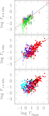 |
Fig. 2. Bottom panel: radio flux at 1.4 GHz of sources in the White et al. (2019) catalog vs. the flux at 24 μm of the associated MIR sources, color coded as in Fig. 1. Flux units are mJy. The star symbols indicate the presence of identified SNRs in the region. Middle panel: radio flux at 5 GHz computed using the spectral index of each radio source in the catalog. We show only data for b-and c-type sources with the continuum line that is the best fit to them. Upper panel: radio flux at 6.3 GHz from aperture photometry of b- and c-type MIR sources with no cataloged radio counterpart but covered by the 6.3 GHz survey. Color coding is the same as in the other panels although cross symbols are used for these sources. The continuum line is the same as in the middle panel while the dashed line is the fit to all data in the middle and upper panels. |
Radio continuum and MIR radiation are both linked to the formation of massive stars and a nearly linear correlation is expected when integrated over the full extent of the galaxy. The ultraviolet radiation from massive stars is partially absorbed by dust and ionizes the surrounding ISM where thermal electrons give rise to free-free emission, while shocks from winds and SNRs produce cosmic rays that emit nonthermal (synchrotron) radiation. However, variations in dust abundance and magnetic field strength justify possible deviations from a linear relation. Integrated over the whole galaxy, the average ratio between the 24 μm and the radio flux density at 1.4 GHz is lower than what we find in most star forming regions of M 33 (Huynh et al. 2010; Appleton et al. 2004). Only regions hosting a SNR show ratios similar to galaxy integrated values. This can be attributed to the noncontinuous production of cosmic rays which diffuse away from star formation sites, but also to the nature of 24 μm emission, which is more enhanced where massive stars form and less diffuse than other IR tracers. However, in M 33 dust opacity in star forming regions is not high enough to absorb most of the ultraviolet and optical starlight (Verley et al. 2009), and 24 μm radiation alone does not trace star formation accurately. The dust abundance, like gas phase metal abundances (Magrini et al. 2010), decreases with galactocentric distance and this variation also drives the sublinear relation between the 24 μm emission and radio continuum. The lack of strong spiral arms in the regions beyond corotation (Corbelli et al. 2019) favors the birth of small star forming sites with a lower MIR-to-radio emission ratio, closer to what is found for galaxies on a larger scale. The open blue circles at the faint end of the distribution in Fig. 2 show examples of this type of YSC; they lie mostly in the outer disk where CO lines are weaker and have no identified GMCs.
3.2. Radio continuum photometry of undetected counterparts
We now consider all the MIR sources which are associated with a GMC or that have an optical counterpart and are very likely star forming regions in the M 33 disk. Those are listed as sources type-b, c, and d in the classification scheme of Corbelli et al. (2017, see their Table 2) and are 526 in total, 300 of which have an associated radio source. To complement the existing radio catalog by deeper searches for diffuse radio emission associated with the remaining MIR sources, we carried out aperture photometry on the radio map at 6.3 GHz. This covers a smaller region than the 5 GHz and 1.4 GHz maps and hence a substantial fraction (about 30% of the total) of the MIR sample lies outside this map.
Of the sources inside the map which had no radio counterpart in the catalog, we detect 90% of them using aperture photometry. By adding the number of detected MIR sources with aperture photometry to the number of matched sources listed in catalogs we have a radio counterpart for 440 MIR sources. Inside the 6.3 GHz map we can claim a detection rate of 95% including cataloged and noncataloged radio counterparts. Given the fact that the nondetected sources are small and affected by beam dilution, and moreover some might have had a bright radio source nearby that artificially affected the estimated background, we can say that MIR sources located in the inner disk (at R < 4 kpc) and related to star-forming regions have associated radio emission. The fraction of MIR sources with a radio counterpart at larger radii is > 60% but we cannot better constrain this number because of the limited coverage of the 6.3 GHz map.
In the upper panel of Fig. 2, we show the radio flux recovered by aperture photometry on the 6.3 GHz map versus the 24 μm flux of MIR star-forming sources with no cataloged radio counterpart. The dashed line is the fit to all sources in the middle and upper panels of the figure. Its slope is 0.80, slightly steeper than the fit relative to matched cataloged sources only. Clearly, YSCs without a cataloged radio counterpart have weaker radio fluxes than YSCs with similar MIR fluxes. This is also because most of these sources are still embedded and are in the early phases of star formation prior to the onset of winds and shocks with enhanced turbulent magnetic fields and cosmic ray acceleration. However, there is a good agreement of the radio fluxes recovered via aperture photometry at 6.3 GHz with those recovered by source extraction at slightly lower frequency. This proves that indeed there is only a unique population of YSCs in M 33 and that the relation between the radio-continuum at 6.3 GHz and the MIR flux is slightly sublinear, with the MIR flux increasing faster than the radio flux as the YSCs becomes brighter.
4. Thermal and nonthermal radio continuum emission
In this section we investigate the fraction of radio emission that is linked to thermal and nonthermal processes in YSCs. To derive the thermal fraction in YSCs we use the extinction corrected Hα flux. This was computed using the expression of the free-free absorption coefficient in the Rayleigh-Jeans regime with the velocity-averaged Gaunt factor given by Draine (2011) and assuming that hydrogen atoms provide most of the ions and free electrons:
 (1)
(1)
where ν is the frequency in GHz, T is the electron temperature in K, and ne and ni are the electron and ion densities in cm−3. The brightness temperature is the product of the electron temperature and the optical depth τν, the latter being the integration of kν along the line of sight. Using the emission measure EM in cm−6 pc we can write the brightness temperature for free-free emission as:
 (2)
(2)
The flux density for a source of uniform brightness is
 (3)
(3)
with kB the Boltzmann’s constant, c the speed of light, and Ωs the angular extent of the source. Using the above expression for the brightness temperature, the flux density in milliJanskys is
 (4)
(4)
The intensity of Hα line emission Dong & Draine (2011) is
 (5)
(5)
In order to recover FHα, the Hα flux over the extent of the source, we multiply the above expression by Ωs. We can then write the free-free flux density in milliJanskys as a function of FHα in ergs cm−2 s−1 as
 (6)
(6)
where we have defined y(T) = 0.619 + 0.031ln(T/104).
4.1. The correlation between Hα and radio continuum emission
Hereafter, we use the Hα flux values measured by our aperture photometry centered on radio sources which are in good agreement with those of Sharma et al. (2011) centered on MIR sources. The correlation between Hα fluxes from our aperture photometry measurements and fluxes at 5 GHz for radio sources associated to YSCs are shown in Fig. 3. The dashed line indicates the expected radio emission from the thermal free-free radiative process. This was recovered using Eq. (6) for an average electron temperature of 104 K across the star forming disk of M 33. In the left panels we have not corrected the Hα line for internal extinction (the Galactic extinction is negligible in the direction of M 33).
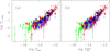 |
Fig. 3. Hα fluxes in erg cm−2 s−1 measured through aperture photometry at the location of radio sources associated with MIR emission shown in panel a as a function of the radio flux recovered from catalogd data at 5 GHz in mJy. Color coding is the same as in Fig. 1 but open symbols have been used. Right panel b: display for the same sources the Hα flux corrected for internal extinction. Filled symbols indicates radio fluxes from aperture photometry at 6.3 GHz of b- and c-type MIR sources with no catalogd radio counterpart. The predicted Hα emission if the radio flux were due to free-free radiation only is shown with a dashed line. The star symbols indicate the presence of identified SNR in the regions (catalog code > 8). |
We use the MIR emission to correct the Hα for internal extinction according to Kennicutt et al. (2009) as follows:
 (7)
(7)
 (8)
(8)
where FHα and F24 are the Hα and 24 μm emission observed and C is a correction factor which takes into account the different MIR and radio source radius. The extent of MIR sources is usually larger than the associated radio sources for large fluxes and therefore we correct the 24 μm flux values given by Sharma et al. (2011) for the different source extent using the factor C equal to the ratio of the radio-to-MIR source area. In the right panel of Fig. 3 we show the extinction-corrected Hα flux associated to YSCs. These corrections are especially important for MIR sources associated with GMCs because extinction corrections here are larger, although for M 33 these are never very large. In Fig. 3 we add the 6.3 GHz radio continuum and Hα fluxes for MIR sources without radio cataloged counterparts for which the radio flux at 6.3 GHz has been recovered by aperture photometry. A comparison between the left and right panels in Fig. 3 shows that extinction corrections are particularly relevant for embedded YSCs. The e-type sources, which are not shown in the figure, do not follow the general correlation and this confirms that these are likely background galaxies. Figure 3 underlines again that small and dimmer YSCs in M 33 have both radio continuum and Hα emission, although resolution and sensitivity limits imply that often these cannot be recovered using source-extraction algorithms. The relation is in agreement with that found for brighter sources and hence we conclude that they belong to the same population.
The correlation between Hα and radio fluxes extend over four orders of magnitude. The expected thermal radio emission as inferred from Hα using Eq. (6), is shown with a dashed line also in panel b. The radio flux associated with star forming regions is two times stronger on average than would be expected if only thermal radio emission were associated with the YSCs. We notice the unambiguous presence of nonthermal emission in MIR sources with Hα flux greater than 2 × 10⁻¹³ erg s−1 cm−2 which correspond to a luminosity of 2 × 1037 erg s−1 at the distance of M 33, equivalent to a cluster populated with stars up to O7-type. Indeed, theoretical computations predicts that only O-type stars more massive than M* are able to produce a wind and therefore a shock. Despite the fact that the value M* is still debated, it is close to that of O7-O6 spectral type (Vink et al. 2000; Marcolino et al. 2009; Muijres et al. 2012).
4.2. Possible dependencies of nonthermal fractions on source compactness and galactocentric distance
In what follows we refine our computation to investigate the variations of thermal and nonthermal fractions with the luminosity, age, and local environment of the star forming regions. The electron temperature needed to estimate the free-free emission can be measured in HII regions through spectroscopy of auroral lines. For M 33 Magrini et al. (2010), have derived how this temperature increases with galactocentric radius. Expressing the latter in kiloparsec, the radial dependence of the electron temperature in M 33 reads:
 (9)
(9)
Below, we measure the total radio flux and the corresponding Hα flux by performing aperture photometry both on the 5 GHz map and on the Hα map, the latter smoothed to the resolution of the radio map. We consider only YSCs of c-type, that is, MIR sources with a radio counterpart in the catalog of White et al. (2019) which are no longer fully embedded in the native molecular cloud but have an optical or FUV counterpart. We divide these YSCs into three categories according to their radius Rs: small for 3 ≤ Rs < 6 arcsec, medium for 6 ≤ Rs < 9 arcsec, and large for 9 ≤ Rs < 18 arcsec. The radius Rs is the average between source semiminor and semimajor axes at 1.4 GHz as listed in the catalog of White et al. (2019). The nonthermal component is simply the difference between the total radio flux and the thermal component, the latter being computed using Eq. (6) with the radially dependent electron temperature Te. To check that the resulting nonthermal fractions do not depend to a significant degree on the aperture, we vary the aperture size but consistently use the same aperture on both maps and compute both backgrounds in annuli placed at distances of 3–3.5 times the source radius.
Figure 4 shows the resulting nonthermal-to-total-radio-flux ratio as a function of the 5 GHz radio flux density F5 GHz. This is the total flux density in mJy in a circular aperture of Rap = 1.5Rs radius. Small, medium, and large sources are displayed in the top, middle, and bottom rows respectively. The histograms to the left show the number of sources in each flux bin. The central panel shows the median (filled triangles) and the mean (open circles) nonthermal fractions with their standard deviations for each flux bin. The green, blue, and magenta colors indicate apertures with radii of 1,1.5, and 2 Rs respectively. We see that there is a common trend for all apertures for both the mean and median values. We also checked our results using photometric fluxes with no background subtraction. Large sources show no clear dependence of the nonthermal fraction on radio flux density and have lower fractions than more compact sources of the same luminosity. An increase of the mean and median nonthermal fractions as a function of radio flux density are clearly seen for medium and small source sizes. The most compact sources brighter than 0.3 mJy show the steepest rise with radio flux density. These sources do not host cataloged SNRs but have nonthermal fractions > 50% at 5 GHz. Faint radio sources in low-mass YSCs have a large dispersion around the mean because of the stochastic character of the initial mass function (IMF, Corbelli et al. 2009) which implies that low-mass YSCs only occasionally host massive stars. Star-forming regions with a large nonthermal to thermal radio flux ratio follow the high-surface-density knots of gaseous filaments while the others are more coarsely placed around or on the filaments.
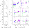 |
Fig. 4. Nonthermal fraction at 5 GHz of radio sources associated with MIR sources in exposed HII regions shown in (a1) for small sources, in (b1) for medium sources, and in (c1) for large sources as a function of the radio flux density at the same frequency. Filled triangles are the median values and open circles are the mean values with the standard deviations. Colors indicate different apertures: green for Rap = Rs, blue for Rap = 1.5Rs and magenta for Rap = 2Rs. Left panels: number of sources in each bin for sources of small (top), medium (middle), and large (bottom) size. Right panels: nonthermal fractions for Rap = Rs (open green circles), in the annulus between Rs and 1.5Rs (open blue squares) and between 1.5Rs and 2Rs (open magenta squares) for small, medium, and large sources (a2, b2, c2 respectively). Radio flux units are mJy. |
In the last panel of Fig. 4, we plot again the mean nonthermal fraction in apertures with Rap = Rs (green color). We add to these points the mean nonthermal fraction in the annulus between 1 and 1.5 Rs (blue color) and between 1.5 and 2 Rs (magenta color). We can see, by comparing panel (a1) and (a2), that the excess of nonthermal flux for compact bright sources is close to the peak of the emission (shown by the green circles) since the external annuli (in magenta) have lower nonthermal fractions. There is no consistent monotonic trend for variations of nonthermal fractions with distance from the radio emission peaks, and no obvious correlation with the radio spectral index given in the catalog.
In the two panels of Fig. 5 we show the correlations between the thermal and nonthermal radio continuum at 5 GHz and the 24 μm emission. The linear relations in the log–log plane have slopes of 0.50 and 0.68 for the thermal and nonthermal radio emission respectively (obtained by minimizing distances of data points to a straight line). The larger scatter at low luminosities in the nonthermal radio continuum–MIR correlation is likely due to noncontinuous injections of fast particles and to stochastic sampling of the upper end of the stellar IMF which settles in as the cluster mass decreases (Corbelli et al. 2009). Turbulent magnetic field amplification and CR acceleration clearly depend on the presence of shocks related to massive stars and might be enhanced in some low-luminosity star-forming regions that host massive star outliers. The slope of the relation is similar to what Basu et al. (2017) find when sampling IC10 at 6.2 GHz on 55 pc scale. The thermal radio continuum declines more slowly with the YSC MIR luminosity than the nonthermal component does. The MIR sources are not overlapping completely with their radio continuum counterparts and in particular they are larger for bright sources. This implies that the total Hα flux corresponding to the MIR source might be stronger in the whole star forming region than what is plotted in Fig. 5, which refers to the location of the radio source. An additional diffuse radio thermal component might be present for bright sources which would make the MIR–thermal-radio-continuum correlation steeper. This can be checked in the future at larger scales using radio maps corrected for short spacing.
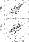 |
Fig. 5. Correlations between the nonthermal (a) and thermal (b) radio continuum at 5 GHz with the 24 μm emission in 248 exposed HII regions of M 33. The lines are linear fits which minimize the distances of data points to straight lines and have slopes of 0.68 and 0.50 in panels a and b respectively. Radio flux units are mJy and have been measured using circular apertures with Rap = 1.5Rs. |
In Fig. 6 we show the galactocentric radial dependencies of the MIR-to-radio continuum, MIR-to-thermal radio continuum, and nonthermal-to-thermal radio continuum ratios. The green dashed lines are plotted for reference and indicate the median value of the distributions. The radial slopes in the bottom two panels of Fig. 6 are similar and driven by the radial decrease of dust abundance, which is particularly evident beyond 3.5 kpc Sources with Fth/Fnth > 1 at 5 GHz make up 40% of the total number of sources at R < 3.5 kpc. This percentage decreases to 25% for R > 3.5 kpc. Nonthermal emission therefore increases with galactocentric distance although the electron temperature in HII regions increases as well to power thermal emission. This result is consistent with a decrease in the radio thermal fraction on a larger scale going radially outwards in M 33 (Tabatabaei et al. 2007b).
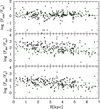 |
Fig. 6. Radial trend of MIR-to-radio flux ratio at 5 GHz (bottom) for the thermal radio emission only (middle), and the nonthermal-to-thermal ratio at 5 GHz (top), plotted for exposed YSCs with radio counterparts in the catalog. Dashed green lines are reference lines placed at the median value of the distributions. |
5. Radio continuum from giant molecular clouds
One of the most striking aspects of the radio emission is how it follows star formation. This is true for both thermal and nonthermal emission. In Fig. 7 we compare the radio emission at 1.4 GHz with the thermal dust emission at 24 μm in two kiloparsec-size arm regions, one on the northern side and the other on the southern side.
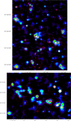 |
Fig. 7. Radio and MIR emission of a kiloparsec-size region allowing details of tens of parsecs in size to be seen. Color image is 1.4 GHz radio emission from White et al. (2019) shown with a log scale of a portion of the northern (upper panel) and southern (bottom panel) side of M 33. Contours are 24 micron Spitzer emission at 1, 3, and 10 (thick blue line) MJy/sr. |
By zooming into regions of 100 pc in size, we can investigate the radio emission from individual GMCs and how this relates to other tracers of star formation. Each GMC covers a well-defined region in the sky (e.g., Fig. 4 of Corbelli et al. (2017)) and we now discuss the radio emission from the GMC sample using photometry of the regions within the cloud boundaries. We exclude clouds outside the 5 GHz map and in the proximity of NGC 604 from the statistical analysis.
We compute both the total radio emission and the residual emission for each GMC. Residual emission has been estimated after subtracting the flux of radio sources in the catalog of White et al. (2019) associated with each GMC, FGMC − Fsrcs, considering radio sources within the average cloud radius. For individual clouds, the residual emission can be negative if for example the radio source is close to the cloud boundary because some flux might not be within the GMC contour. Table 1 lists for each cloud class the median ( ) and mean (
 ) fluxes at 5 GHz, and the median and mean residual emission (
 and
and  respectively). In addition we show the mean mass of GMCs, and the median and mean Hα and 24 μm fluxes for each cloud class. Radio emission is clearly detected for most of the clouds with exposed star formation (C class) with a wide dispersion: fluxes are distributed mostly between the values of 50 and 5000 μJy at 5 GHz with a median value of 282 μJy. Radio emission at 5 GHz is detected for about 80% of B-type clouds with most of the fluxes being between 50 and 500 μJy and a median value of 20 μJy, much lower than for C-type clouds. For inactive clouds, or GMCs without massive star formation (A class), radio fluxes are distributed around the value of zero.
Median and mean radio fluxes at 5 GHz, and Hα and 24 μm emission for each GMC class.
The low detection rate of clouds without star formation is interesting but requires further investigation using radio maps corrected for missing short spacing. Molecular clouds are expected to concentrate magnetic fields, which could result in some diffuse nonthermal emission if cosmic rays penetrate the clouds. There are three A-type clouds next to NGC 604 which show enhanced radio emission and a double peak in the CO J = 1 − 0 line. Strong shocks in the expanding shell of NGC 604 likely compress the surrounding ISM, favoring the formation of GMCs and the propagation of relativistic particles streaming along the magnetic field lines. In a future paper dedicated to the mechanism for CR acceleration we will use radio maps corrected for short spacing to examine diffuse radio emission in GMCs in more detail at various stages of evolution and at different locations in the disk.
Residual emission not associated with identified radio sources is barely present in B-type clouds but represents about one-third of the total radio emission for GMCs of class C with exposed star formation. As star formation progresses, and the GMC becomes C-type with the YSC breaking through the cloud, the increase of radio emission in GMCs is much stronger than any corresponding increase of thermal emission (as indicated by Hα recombination lines or hot dust emission). As shown in Table 1, both Hα and 24 μm emission increase only by a few from B- to C-class clouds. The average radio emission instead increases by more than one order of magnitude suggesting a substantial increase of the nonthermal component as the YSC evolves. In Fig. 8 we show the correlation between the radio and the Hα flux from GMCs; in the right panel we have binned the GMCs according to their Hα emission. An average correction for extinction has been applied to the Hα emission from GMCs using Eq. (8), where all fluxes refer to integrated quantities inside each GMC contour. The trend for the red dots, which indicate clouds with exposed star formation (C-type), is very similar to what we find for individual YSCs. Figure 8 highlights the weaker radio emission of A- and B-type GMCs (magenta and green dots respectively). The large dispersion, as indicated by the error bars, is due both to variations of the star formation rate in GMCs and to some side lobe affecting the 5 GHz map.
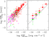 |
Fig. 8. Left panel: radio continuum at 5 GHz vs. the Hα emission for each GMC. Right panel: mean radio emission from GMCs in bins of Hα. An average correction for extinction, using the 24 μm emission associated with each cloud, has been applied to the Hα flux of individual GMCs. Red circles indicate C-type clouds with exposed YSCs, green circles show B-type clouds with embedded star formation, and magenta circles show inactive clouds of A-type. Only data for GMCs detected at 5 GHz have been used. The dashed line shows the expected thermal component at 5 GHz |
6. The link between radio emission and star formation
In the previous section we show that thermal radio emission in HII regions can be estimated from recombination lines such as Hα and we used the 24 μm flux density to correct Hα for internal extinction (generally low for exposed YSCs in M 33). Extinction- corrected Hα emission provides an estimate not only of the thermal radio flux density but also of the local star formation rate. For the scales we are examining here, from GMCs to YSCs, star formation takes place over a timescale that is shorter than the GMC lifetime, which itself is estimated to be on the order of 14 Myr (Corbelli et al. 2017). YSCs start breaking through the cloud when they are about 5 Myrs old, after the embedded phase (Corbelli et al. 2017). Hence, the timescales involved when sampling GMCs and YSCs are on the order of 10 Myr, until the GMC disperses through the ISM. If the stellar mass of the newly formed cluster is not sufficient to fully populate the IMF at its upper end, the Hα is no longer a good star-formation-rate indicator. This affects cluster masses below 103 M⊙ or Hα luminosities lower than 1037 erg s−1, corresponding to a flux of about 10−13 erg cm−2 s−1 at the distance of M 33 (Sharma et al. 2011). At lower luminosities, limitations due to the stochastic sampling of the IMF, which implies occasional formation of massive stars, can be overcome using mean values for an ensemble of sources and not individual source values.
A log–log plot in Fig. 9 shows the distribution of the total radio flux at 5 GHz versus the Hα flux corrected for extinction. The straight line, has a slope 0.93 and a very low dispersion. The dashed green line is the fit to the data if we require a linear relation (a slope of one). The goodness of this fit implies that low-mass star forming regions with Hα < 10−13 erg cm−2 s−1 or F5 GHz < 0.3 mJy are equally dim in radio as in Hα emission. The correlation of Hα brightness with the nonthermal radio flux density shown by the straight line in Fig. 9b has a slope of 0.87 and is less tight. This supports the use of total radio continuum, which does not suffer extinction, as an indicator of the star formation rate (SFR). The following equation (Kennicutt & Evans 2012) links the star formation rate with Hα luminosity:
 (10)
(10)
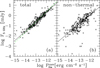 |
Fig. 9. Total (left panel) and nonthermal radio continuum flux (right panel) at 5 GHz for MIR-selected star forming regions plotted as a function of the Hα flux corrected for extinction. The Hα emission appears to be more closely related to the total radio flux than to the nonthermal radio continuum only. The fitted correlations shown are drawn by minimizing distances to the line and their slopes are 0.87 and 0.93 for the total and nonthermal flux respectively. Plotted quantities are relative to circular apertures with Rap = 1.5Rs. The green dashed line is the best fitted line with slope unity. |
This is in general an lower limit due to ionizing photon leakage from star forming regions, a problem which affects also the thermal radio continuum. Using the linear relation (green dashed line) shown in Fig. 9, we can write
 (11)
(11)
We obtain the same expression when fitting the radio continuum flux density at 5 GHz versus Hα emission in GMCs. We can then compare this expression, which applies to discrete events of star formation at small scales, with the SFR integrated over galaxies. Using the far infrared–radio continuum correlation to calibrate the star formation rate in galaxies as a whole (Murphy et al. 2011), the relation reads:
 (12)
(12)
Given the spectral indexes observed for the radio sources (> − 0.5), the ratio between YSC luminosities at 1.4 and 5 GHz is < 2. Hence, for a given SFR, Eq. (12) implies a higher radio continuum luminosity than Eq. (11). That is to say that the ratio between the Hα luminosity and radio continuum luminosity is higher in individual star forming regions than globally for integrated quantities in spiral galaxies. We reach a similar conclusion for the ratio between the MIR emission and radio continuum, as mentioned in Sect. 3, with the exception of a few HII regions. On the other hand it is well known that large-scale radio emission in spiral galaxies has a strong nonthermal radio component (Condon & Yin 1990): magnetic fields are pervasive in the ISM and cosmic rays can quickly diffuse away from where they are injected, supporting our finding.
6.1. Nonthermal radio continuum from YSCs to GMC scale
To further investigate the link between the radio emission and the star formation rate, or how the ratio of thermal to nonthermal radio continuum flux density vary from small to large scales, we now analyze the sample of GMCs. Cloud complexes generally extend over about 100 pc, occupying a larger area than star forming and HII regions, except for very massive YSCs whose HII regions are very extended and have dispersed their native clouds.
The left panels of Fig. 10 show the YSC data, which were also displayed in panels (a1)-to-(c1) of Fig. 4, and the GMC mean values of the nonthermal to total radio continuum ratio. The latter are computed considering only GMCs associated with the YSCs and are shown as a function of the mean radio continuum flux density of the hosted YSCs in each bin. In the middle and top panels, relative to small and medium-size radio continuum sources respectively, we can see that radio-bright YSCs are hosted by GMCs with similar nonthermal-to-total-radio-continuum flux ratios. A few bright compact YSCs have higher nonthermal-to-radio-continuum flux ratios than their host GMCs (Fig. 10a). This confirms our earlier finding, shown in panel (a2) of Fig. 4, that the high nonthermal fractions in these sources decrease when considering a wider area around them. We cannot exclude that the localized excess of nonthermal fractions for a few bright compact radio sources is incorrect because of an underestimation of the free-free emission, which has been considered to be optically thin (Felli & Panagia 1981; Kobulnicky & Johnson 1999; Johnson et al. 2001).
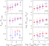 |
Fig. 10. Left panels: nonthermal-to-total-radio-continuum flux density ratio at 5 GHz for radio sources associated to exposed YSCs (blue circles) using apertures with Rap = 1.5Rs for small (a1), medium (b1), and large (c1) sources. In the same panels we show the nonthermal-to-total-radio flux density ratio for the GMCs hosting the YSCs (red squares) as a function of the radio emission of the YSCs. We underline that not all YSCs considered here have an associated GMC. Right panels: total-to-thermal radio flux ratio for the whole ensemble of GMCs hosting exposed YSCs (filled symbols), binned according to their star formation rate per unit area. Radio continuum has been used to estimate the SFR density (red squares). From top to bottom we compare the ratios relative to GMCs with the ratios relative to small, medium, and large sources respectively (open blue circles) binned according to the SFR per unit area. The area around the source is circular with a radius of 1.5Rs. |
For extended radio sources, Fig. 10c1 shows that although the associated GMCs follow the same trend with radio flux density as the associated YSCs, they have higher nonthermal fractions, similar to clouds shown in other panels and hosting more compact sources. In this case, the HII region is comparable to or larger than the GMC and it is expanding while dispersing the parent cloud. It is conceivable that GMCs associated with some of these sources are leftovers or are newly formed, possibly triggered by HII shell expansion.
In the right panels of Fig. 10 we plot in red the total-to-thermal radio flux ratio for the whole ensemble of GMCs hosting exposed YSCs (filled red squares). Data have been binned according to cloud star formation rate per unit area and the same data are displayed in all three panels for a direct comparison with the same ratio measured for small (a2), medium (b2), and large (c2) YSCs (open blue circles). On the x-axis we show the SFR per unit area, as traced by radio emission, computed inside cloud contours for GMCs, and in a circular area with a radius of 1.5Rs for YSCs. On the y-axis we display the log of total-to-thermal flux ratio for a direct comparison with the model discussed by Schleicher & Beck (2016, see their Fig. 10). For discrete star forming sites, such as those we are considering here, the plot shown in Fig. 10 confirms that the total-to-thermal radio flux ratio increases with star formation density for compact YSCs and clouds, but there is a flattening for clouds with ΣSFR > 0.03 M⊙ yr−1 kpc−2. The extended sources show a remarkably constant ratio of F5 GHz/Fth with an equal share between the thermal and nonthermal flux density. The model of Schleicher & Beck (2016) on a larger scale and for a continuous star formation rate predicts an increase of the total-to-thermal radio flux ratio with ΣSFR faster than what we observe for compact star forming regions or GMCs. Schleicher & Beck (2016) explain the increasing trend as being due to turbulent magnetic field amplification by star formation. However, as the authors point out, discrete injection events cannot maintain a correlation between star formation rate and magnetic field strength. As a consequence, and given also the higher frequency we are sampling, the slower increase of the total-to-thermal radio flux ratio with star formation in our data is understandable. The relation between star formation rate and total-to-thermal radio flux ratio is lost if we trace the SFR density using Hα emission. This underlines the presence of fluctuations in the strength of radiative processes in individual YSCs due to stochastic events of massive star formation.
6.2. Cosmic ray diffusion and the YSC contribution to nonthermal emission of M 33
At scales smaller than 1 kpc Tabatabaei et al. (2013b) conclude that a turbulent magnetic field of order 8 μG dominates over the ordered component in M 33, and this tangled field implies that cosmic rays diffuse over a relatively short path length, smaller than 400 pc, during their lifetime. The CRs are expected to be transported via streaming instabilities at the Alfvén speed  . The average gas volume density in the giant cloud complexes we are considering is on the order of 10−23 gr cm−3 although individual molecular clouds in them, where stars form, have higher densities. For the duration of the star formation phase in GMCs, which is on the order of 10 Myr, the CRs can then diffuse over 70 pc, which is comparable to GMC sizes. Bright and compact YSCs, which have not yet aged, are producing massive stars with discrete injection of CRs: these lag in the surrounding cloud increasing the nonthermal fraction of the cloud radio emission. For extended HII regions no longer surrounded by molecular gas, the gas density is lower and locally produced CRs diffuse out quickly. As injections of CRs stop, the local nonthermal radio continuum emission decreases.
What is the fraction of the global nonthermal emission of M 33 that is in discrete sources such as YSCs or SNRs? Tabatabaei et al. (2007b) measured the total radio emission of M 33 at 4.8 GHz and find that the total flux is 1.3 Jy. The total Hα flux of M 33 corrected for extinction is about 5 × 10⁻¹⁰ erg s−1 cm−2 (Verley et al. 2009), which implies that about one-third of the emission of M 33 at 5 GHz is thermal and the remaining two-thirds are due to nonthermal processes. The mean nonthermal radio continuum emission of SNRs and YSCs identified in this paper are similar (0.6 mJy) but SNRs in the radio catalog of White et al. (2019) are less numerous than YSCs. The contribution of identified SNRs to the total nonthermal flux of M 33 at 5 GHz is 9%, while twice as much, 19%, is localized around YSCs hosting no known SNRs but having MIR counterparts. Considering some additional contribution by radio continuum sources associated with more evolved HII regions which lack a MIR counterpart, we estimate that at least one-third of the total nonthermal emission at 5 GHz is linked to discrete current injection events of CRs connected with the evolution of massive stars. Diffusion of CRs into the ISM from the ongoing and past generation of massive stars must account for the remaining fraction.
The mean global star formation density in M 33 is 0.0032 M⊙ yr−1 kpc−2, and the ratio of total-to-thermal flux is 5.7 at 1.4 GHz (Tabatabaei et al. 2007c). This estimate is in very good agreement with that predicted by the model by Schleicher & Beck (2016) for a continuous star formation law.
7. Summary
The formation of stars can be traced using FUV stellar continuum, gas recombination lines such as Hα, radio thermal and nonthermal continuum, and MIR emission of hot dust grains which absorb the radiation of the newly formed stars. For star forming galaxies, a tight linear relation is seen between their IR emission and radio continuum luminosities. At present, high-angular-resolution surveys of the whole star forming disk of the closest galaxies allow investigation of such relations in individual molecular clouds as the formation of YSCs proceeds, and down to spatial scales below 50 pc. In this paper, we explore the MIR, radio continuum, and Hα emission for a large sample of star forming regions in M 33 (526 YSCs) and for their native molecular clouds. The YSC candidates have been selected for their MIR hot dust emission at 24 μm (Sharma et al. 2011). Using a radio continuum source catalog in the M 33 sky area (White et al. 2019) we find radio counterparts at 1.4 and 5 GHz for more than half of the YSCs. We use high-sensitivity maps at 6.3 GHz to successfully measure radio emission for the most diffuse and weak sources without a cataloged counterpart.
The radio continuum luminosity of a star forming region shows a correlation with the 24 μm luminosity of the associated hot dust component, whose slope is sublinear in the log–log scale. The 24 μ luminosity of YSCs fully embedded in the native molecular clouds follows a similar correlation with the radio continuum. We highlight the fact that previous attempts to discover embedded star forming sources in M 33 through radio-continuum surveys were unsuccessful (Buckalew et al. 2006). Thanks to sensitive radio continuum maps at 6.3 GHz we have been able to confirm, for the first time in a nearby spiral galaxy, the embedded nature of many YSCs associated with molecular clouds with no optical or FUV counterpart. Given the variations of the spatial distribution of grains in the HII regions and of the stellar continuum fraction absorbed by dust, it is quite surprising to find a relation that holds for the overall YSC population, from the embedded to the exposed phase, from the central region to the galaxy outskirts.
The slow chemical enrichment of galaxies with cosmic time and the variety of processes that regulate the life cycle and temperature of dust grains implies that 24 μm emission alone might not be sufficient to trace star formation. A combined tracer, that is, IR with FUV or hydrogen recombination lines, has become a commonly used star formation rate estimator (Kennicutt et al. 2009). We show here that the correlation between the radio continuum at 5 GHz and the combined tracer 24 μm and Hα emission (or extinction corrected Hα) holds over four orders of magnitude at scales between a few tens and ∼100 pc. The relation is close to linear and extremely tight when data on YSCs refer only to the latest stage of evolution in the host molecular cloud (exposed phase). The correlation is tighter if the total radio continuum is considered rather than the nonthermal radio component. We have used the Hα line to estimate the thermal free-free emission assuming an optically thin medium. In examining individual YSCs of low luminosities, stochastic sampling of the IMF at its high mass end increases the dispersion in the relation between hot dust emission and nonthermal radio continuum due to stronger variations of turbulent magnetic field amplification and CR production.
We find a significant fraction of the 5 GHz emission to be thermal, but more than half of the radio emission from compact radio-bright YSCs is attributable to nonthermal processes. The unambiguous nonthermal emission in star forming regions where the Hα flux is greater than 10−13 erg s−1 cm−2, even in the absence of a SNR, implies ubiquitous local production of cosmic rays when the YSC has at least one O7-type star. Indeed, theoretical computations predict that these O-type stars are able to produce a wind and therefore a shock. At least one-third of the total nonthermal emission of M 33 at 5 GHz (from over 380 sources) is linked to discrete current injection events of CRs connected with massive stars in YSCs or SNRs.
In GMCs the radio continuum correlates with the extinction corrected Hα emission following a similar trend as for individual star forming regions As determined by Corbelli et al. (2017), the duration of the life cycle for M 33 molecular clouds is about 14 Gyr with the mean molecular cloud mass that increases only by a factor three going from the initial inactive phase, through the embedded phase, to the exposed phase prior to cloud dispersal. The radio emission of the whole GMC shows a stronger increase as star formation progresses due to the nonthermal component which becomes ubiquitous as the YSC starts breaking through the cloud. Inactive GMCs or molecular clouds hosting only embedded sources or faint YSCs have much lower radio continuum luminosities.
Extended radio sources, likely associated with evolved HII regions, do not show a correlation between the nonthermal fraction and radio luminosity, and have on average lower nonthermal fractions than more compact sources. We interpret this trend as due to fast diffusion of CRs as the HII shell expands well beyond the native cloud, with CR injections becoming more rare at a later stage of the cluster evolution. Diffusion of CRs can also explain the lower ratios between the radio continuum at 5 GHz and the 24 μm or Hα emission in individual star forming regions of M 33 compared to those measured for galaxies as a whole in the local universe.
The nonthermal fraction correlates with the total radio continuum luminosity for compact YSCs and GMCs with exposed star formation. The shallow increase of the total-to-thermal radio flux ratio with star formation density in compact YSCs and in GMCs is in agreement with theoretical models of star-formation-induced turbulent magnetic field amplification. Tangled magnetic field in turbulent molecular complexes can prevent fast diffusion of CR electrons to larger scales during GMC lifetime (Tabatabaei et al. 2013b). Future deep radio surveys that trace the diffuse radio emission and specific theoretical modeling of fluctuations in CR injections during star formation events can help to shed light on the link between small- and large-scale radio continuum emission in galaxies.
Acknowledgments
EC acknowledges the support from grant PRIN MIUR 2017 - 20173ML3WW001 and from the INAF PRIN-SKA 2017 program 1.05.01.88.04.
References
- Aharonian, F., Yang, R., & de Oña Wilhelmi, E. 2019, Nat. Astron., 3, 561 [NASA ADS] [CrossRef] [Google Scholar]
- Appleton, P. N., Fadda, D. T., Marleau, F. R., et al. 2004, ApJS, 154, 147 [NASA ADS] [CrossRef] [Google Scholar]
- Basu, A., Roychowdhury, S., Heesen, V., et al. 2017, MNRAS, 471, 337 [CrossRef] [Google Scholar]
- Bell, E. F. 2003, ApJ, 586, 794 [Google Scholar]
- Buckalew, B. A., Kobulnicky, H. A., Darnel, J. M., et al. 2006, ApJS, 162, 329 [NASA ADS] [CrossRef] [Google Scholar]
- Cesarsky, C. J., & Montmerle, T. 1983, Space Sci. Rev., 36, 173 [NASA ADS] [CrossRef] [Google Scholar]
- Condon, J. J., & Yin, Q. F. 1990, ApJ, 357, 97 [NASA ADS] [CrossRef] [Google Scholar]
- Corbelli, E., Verley, S., Elmegreen, B. G., & Giovanardi, C. 2009, A&A, 495, 479 [NASA ADS] [CrossRef] [EDP Sciences] [Google Scholar]
- Corbelli, E., Braine, J., Bandiera, R., et al. 2017, A&A, 601, A146 [NASA ADS] [CrossRef] [EDP Sciences] [Google Scholar]
- Corbelli, E., Braine, J., & Giovanardi, C. 2019, A&A, 622, A171 [CrossRef] [EDP Sciences] [Google Scholar]
- Cotton, W. D. 2008, PASP, 120, 439 [NASA ADS] [CrossRef] [Google Scholar]
- Cotton, W. D., Condon, J. J., Kellermann, K. I., et al. 2018, ApJ, 856, 67 [NASA ADS] [CrossRef] [Google Scholar]
- Dong, R., & Draine, B. T. 2011, ApJ, 727, 35 [NASA ADS] [CrossRef] [Google Scholar]
- Draine, B. T. 2011, Physics of the Interstellar and Intergalactic Medium [Google Scholar]
- Dumas, G., Schinnerer, E., Tabatabaei, F. S., et al. 2011, AJ, 141, 41 [NASA ADS] [CrossRef] [Google Scholar]
- Felli, M., & Panagia, N. 1981, A&A, 102, 424 [NASA ADS] [Google Scholar]
- Freedman, W. L., Wilson, C. D., & Madore, B. F. 1991, ApJ, 372, 455 [NASA ADS] [CrossRef] [Google Scholar]
- Gieren, W., Górski, M., Pietrzyński, G., et al. 2013, ApJ, 773, 69 [NASA ADS] [CrossRef] [Google Scholar]
- Gordon, S. M., Duric, N., Kirshner, R. P., Goss, W. M., & Viallefond, F. 1999, ApJS, 120, 247 [NASA ADS] [CrossRef] [Google Scholar]
- Gratier, P., Braine, J., Rodriguez-Fernandez, N. J., et al. 2012, A&A, 542, A108 [NASA ADS] [CrossRef] [EDP Sciences] [Google Scholar]
- Greenawalt, B. E. 1998, Ph.D. Thesis, New Mexico State University, USA [Google Scholar]
- Helou, G., Soifer, B. T., & Rowan-Robinson, M. 1985, ApJ, 298, L7 [Google Scholar]
- Hoopes, C. G., & Walterbos, R. A. M. 2000, ApJ, 541, 597 [NASA ADS] [CrossRef] [Google Scholar]
- Hughes, A., Wong, T., Ekers, R., et al. 2006, MNRAS, 370, 363 [NASA ADS] [CrossRef] [Google Scholar]
- Huynh, M. T., Gawiser, E., Marchesini, D., Brammer, G., & Guaita, L. 2010, ApJ, 723, 1110 [NASA ADS] [CrossRef] [Google Scholar]
- Johnson, K. E., Kobulnicky, H. A., Massey, P., & Conti, P. S. 2001, ApJ, 559, 864 [NASA ADS] [CrossRef] [Google Scholar]
- Kennicutt, R. C., & Evans, N. J. 2012, ARA&A, 50, 531 [NASA ADS] [CrossRef] [Google Scholar]
- Kennicutt, R. C. J., Hao, C. N., & Calzetti, D. 2009, ApJ, 703, 1672 [NASA ADS] [CrossRef] [Google Scholar]
- Kobulnicky, H. A., & Johnson, K. E. 1999, ApJ, 527, 154 [NASA ADS] [CrossRef] [Google Scholar]
- Lee, J. H., & Lee, M. G. 2014, ApJ, 793, 134 [CrossRef] [Google Scholar]
- Long, K. S., Blair, W. P., Winkler, P. F., et al. 2010, ApJS, 187, 495 [NASA ADS] [CrossRef] [Google Scholar]
- Magrini, L., Stanghellini, L., Corbelli, E., Galli, D., & Villaver, E. 2010, A&A, 512, A63 [NASA ADS] [CrossRef] [EDP Sciences] [Google Scholar]
- Marcolino, W. L. F., Bouret, J. C., Martins, F., et al. 2009, A&A, 498, 837 [NASA ADS] [CrossRef] [EDP Sciences] [Google Scholar]
- Muijres, L. E., Vink, J. S., de Koter, A., Müller, P. E., & Langer, N. 2012, A&A, 537, A37 [NASA ADS] [CrossRef] [EDP Sciences] [Google Scholar]
- Murphy, E. J., Condon, J. J., Schinnerer, E., et al. 2011, ApJ, 737, 67 [NASA ADS] [CrossRef] [Google Scholar]
- Padovani, M., Marcowith, A., Sánchez-Monge, Á., Meng, F., & Schilke, P. 2019, A&A, 630, A72 [NASA ADS] [CrossRef] [EDP Sciences] [Google Scholar]
- Parizot, E., Marcowith, A., van der Swaluw, E., Bykov, A. M., & Tatischeff, V. 2004, A&A, 424, 747 [NASA ADS] [CrossRef] [EDP Sciences] [Google Scholar]
- Schleicher, D. R. G., & Beck, R. 2013, A&A, 556, A142 [NASA ADS] [CrossRef] [EDP Sciences] [Google Scholar]
- Schleicher, D. R. G., & Beck, R. 2016, A&A, 593, A77 [NASA ADS] [CrossRef] [EDP Sciences] [Google Scholar]
- Schober, J., Schleicher, D. R. G., & Klessen, R. S. 2016, ApJ, 827, 109 [NASA ADS] [CrossRef] [Google Scholar]
- Sharma, S., Corbelli, E., Giovanardi, C., Hunt, L. K., & Palla, F. 2011, A&A, 534, A96 [NASA ADS] [CrossRef] [EDP Sciences] [Google Scholar]
- Tabatabaei, F. S., Beck, R., Krause, M., et al. 2007a, A&A, 466, 509 [NASA ADS] [CrossRef] [EDP Sciences] [Google Scholar]
- Tabatabaei, F. S., Krause, M., & Beck, R. 2007b, A&A, 472, 785 [NASA ADS] [CrossRef] [EDP Sciences] [Google Scholar]
- Tabatabaei, F. S., Beck, R., Krügel, E., et al. 2007c, A&A, 475, 133 [NASA ADS] [CrossRef] [EDP Sciences] [Google Scholar]
- Tabatabaei, F. S., Krause, M., Fletcher, A., & Beck, R. 2008, A&A, 490, 1005 [NASA ADS] [CrossRef] [EDP Sciences] [Google Scholar]
- Tabatabaei, F. S., Schinnerer, E., Murphy, E. J., et al. 2013a, A&A, 552, A19 [NASA ADS] [CrossRef] [EDP Sciences] [Google Scholar]
- Tabatabaei, F. S., Berkhuijsen, E. M., Frick, P., Beck, R., & Schinnerer, E. 2013b, A&A, 557, A129 [NASA ADS] [CrossRef] [EDP Sciences] [Google Scholar]
- Verley, S., Hunt, L. K., Corbelli, E., & Giovanardi, C. 2007, A&A, 476, 1161 [NASA ADS] [CrossRef] [EDP Sciences] [Google Scholar]
- Verley, S., Corbelli, E., Giovanardi, C., & Hunt, L. K. 2009, A&A, 493, 453 [NASA ADS] [CrossRef] [EDP Sciences] [Google Scholar]
- Vink, J. S., de Koter, A., & Lamers, H. J. G. L. M. 2000, A&A, 362, 295 [Google Scholar]
- White, R. L., Long, K. S., Becker, R. H., et al. 2019, ApJS, 241, 37 [NASA ADS] [CrossRef] [Google Scholar]
All Tables
Median and mean radio fluxes at 5 GHz, and Hα and 24 μm emission for each GMC class.
All Figures
|
Fig. 1. Bottom panel: radio flux at 1.4 GHz of sources in the White et al. (2019) catalog vs. the associated Hα flux in the same catalog. Magenta color highlights sources in the radio catalog which are associated with MIR sources in the catalog of Sharma et al. (2011). Top panel: sources in the radio catalog which are associated with MIR sources hosted by known GMCs (filled green and red symbols) and not associated with known GMCs (open blue and cyan symbols). The color coding, as indicated in the upper left corner, outlines the classification scheme of Corbelli et al. (2017) (see text for details), with blue and red colors marking MIR sources with a clear counterpart in Hα (c-type). |
| In the text | |
|
Fig. 2. Bottom panel: radio flux at 1.4 GHz of sources in the White et al. (2019) catalog vs. the flux at 24 μm of the associated MIR sources, color coded as in Fig. 1. Flux units are mJy. The star symbols indicate the presence of identified SNRs in the region. Middle panel: radio flux at 5 GHz computed using the spectral index of each radio source in the catalog. We show only data for b-and c-type sources with the continuum line that is the best fit to them. Upper panel: radio flux at 6.3 GHz from aperture photometry of b- and c-type MIR sources with no cataloged radio counterpart but covered by the 6.3 GHz survey. Color coding is the same as in the other panels although cross symbols are used for these sources. The continuum line is the same as in the middle panel while the dashed line is the fit to all data in the middle and upper panels. |
| In the text | |
|
Fig. 3. Hα fluxes in erg cm−2 s−1 measured through aperture photometry at the location of radio sources associated with MIR emission shown in panel a as a function of the radio flux recovered from catalogd data at 5 GHz in mJy. Color coding is the same as in Fig. 1 but open symbols have been used. Right panel b: display for the same sources the Hα flux corrected for internal extinction. Filled symbols indicates radio fluxes from aperture photometry at 6.3 GHz of b- and c-type MIR sources with no catalogd radio counterpart. The predicted Hα emission if the radio flux were due to free-free radiation only is shown with a dashed line. The star symbols indicate the presence of identified SNR in the regions (catalog code > 8). |
| In the text | |
|
Fig. 4. Nonthermal fraction at 5 GHz of radio sources associated with MIR sources in exposed HII regions shown in (a1) for small sources, in (b1) for medium sources, and in (c1) for large sources as a function of the radio flux density at the same frequency. Filled triangles are the median values and open circles are the mean values with the standard deviations. Colors indicate different apertures: green for Rap = Rs, blue for Rap = 1.5Rs and magenta for Rap = 2Rs. Left panels: number of sources in each bin for sources of small (top), medium (middle), and large (bottom) size. Right panels: nonthermal fractions for Rap = Rs (open green circles), in the annulus between Rs and 1.5Rs (open blue squares) and between 1.5Rs and 2Rs (open magenta squares) for small, medium, and large sources (a2, b2, c2 respectively). Radio flux units are mJy. |
| In the text | |
|
Fig. 5. Correlations between the nonthermal (a) and thermal (b) radio continuum at 5 GHz with the 24 μm emission in 248 exposed HII regions of M 33. The lines are linear fits which minimize the distances of data points to straight lines and have slopes of 0.68 and 0.50 in panels a and b respectively. Radio flux units are mJy and have been measured using circular apertures with Rap = 1.5Rs. |
| In the text | |
|
Fig. 6. Radial trend of MIR-to-radio flux ratio at 5 GHz (bottom) for the thermal radio emission only (middle), and the nonthermal-to-thermal ratio at 5 GHz (top), plotted for exposed YSCs with radio counterparts in the catalog. Dashed green lines are reference lines placed at the median value of the distributions. |
| In the text | |
|
Fig. 7. Radio and MIR emission of a kiloparsec-size region allowing details of tens of parsecs in size to be seen. Color image is 1.4 GHz radio emission from White et al. (2019) shown with a log scale of a portion of the northern (upper panel) and southern (bottom panel) side of M 33. Contours are 24 micron Spitzer emission at 1, 3, and 10 (thick blue line) MJy/sr. |
| In the text | |
|
Fig. 8. Left panel: radio continuum at 5 GHz vs. the Hα emission for each GMC. Right panel: mean radio emission from GMCs in bins of Hα. An average correction for extinction, using the 24 μm emission associated with each cloud, has been applied to the Hα flux of individual GMCs. Red circles indicate C-type clouds with exposed YSCs, green circles show B-type clouds with embedded star formation, and magenta circles show inactive clouds of A-type. Only data for GMCs detected at 5 GHz have been used. The dashed line shows the expected thermal component at 5 GHz |
| In the text | |
|
Fig. 9. Total (left panel) and nonthermal radio continuum flux (right panel) at 5 GHz for MIR-selected star forming regions plotted as a function of the Hα flux corrected for extinction. The Hα emission appears to be more closely related to the total radio flux than to the nonthermal radio continuum only. The fitted correlations shown are drawn by minimizing distances to the line and their slopes are 0.87 and 0.93 for the total and nonthermal flux respectively. Plotted quantities are relative to circular apertures with Rap = 1.5Rs. The green dashed line is the best fitted line with slope unity. |
| In the text | |
|
Fig. 10. Left panels: nonthermal-to-total-radio-continuum flux density ratio at 5 GHz for radio sources associated to exposed YSCs (blue circles) using apertures with Rap = 1.5Rs for small (a1), medium (b1), and large (c1) sources. In the same panels we show the nonthermal-to-total-radio flux density ratio for the GMCs hosting the YSCs (red squares) as a function of the radio emission of the YSCs. We underline that not all YSCs considered here have an associated GMC. Right panels: total-to-thermal radio flux ratio for the whole ensemble of GMCs hosting exposed YSCs (filled symbols), binned according to their star formation rate per unit area. Radio continuum has been used to estimate the SFR density (red squares). From top to bottom we compare the ratios relative to GMCs with the ratios relative to small, medium, and large sources respectively (open blue circles) binned according to the SFR per unit area. The area around the source is circular with a radius of 1.5Rs. |
| In the text | |
Current usage metrics show cumulative count of Article Views (full-text article views including HTML views, PDF and ePub downloads, according to the available data) and Abstracts Views on Vision4Press platform.
Data correspond to usage on the plateform after 2015. The current usage metrics is available 48-96 hours after online publication and is updated daily on week days.
Initial download of the metrics may take a while.