| Issue |
A&A
Volume 691, November 2024
|
|
|---|---|---|
| Article Number | A199 | |
| Number of page(s) | 19 | |
| Section | Extragalactic astronomy | |
| DOI | https://doi.org/10.1051/0004-6361/202451110 | |
| Published online | 13 November 2024 | |
Radio–FIR correlation: A probe into cosmic ray propagation in the nearby galaxy IC 342
1
School of Astronomy, Institute for Research in Fundamental Sciences (IPM), PO Box 19395-5531 Tehran, Iran
2
Max-Planck Institut für Radioastronomie, Auf dem Hügel 69, 53121 Bonn, Germany
3
Max-Planck Institut für Astronomie, Königstuhl 17, 69117 Heidelberg, Germany
4
Hamburger Sternwarte, Universität Hamburg, Gojenbergsweg 112, 21029 Hamburg, Germany
5
Canadian Institute for Theoretical Astrophysics (CITA), University of Toronto, 60 St George St, Toronto M5S 3H8, Canada
6
INAF – Istituto di Radioastronomia, Via P. Gobetti 101, 40129 Bologna, Italy
7
Ruhr University Bochum, Faculty of Physics and Astronomy, Astronomical Institute (AIRUB), 44780 Bochum, Germany
8
Astronomical Observatory of the Jagiellonian University, ul. Orla 171, 30-244 Kraków, Poland
⋆ Corresponding author; This email address is being protected from spambots. You need JavaScript enabled to view it.
Received:
13
June
2024
Accepted:
15
September
2024
Abstract
Resolved studies of the correlation between the radio and far-infrared (FIR) emission from galaxies at different frequencies can unveil the interplay between star formation and the relativistic interstellar medium (ISM). Thanks to the LOFAR LoTSS observations combined with VLA, Herschel, and WISE data, we study the role of cosmic rays and magnetic fields in the radio–FIR correlation on scales of ≳200 pc in the nearby galaxy IC 342. The thermal emission traced by the 22 μm emission, constitutes about 6%, 13%, and 30% of the observed radio emission at 0.14, 1.4, and 4.8 GHz, respectively, in star-forming regions and less in other parts. The nonthermal spectral index becomes flatter at frequencies lower than 1.4 GHz (αn = −0.51 ± 0.09, Sν ∝ ναn) than between 1.4 and 4.8 GHz (αn = −1.06 ± 0.19) on average, and this flattening occurs not only in star-forming regions but also in the diffuse ISM. The radio–FIR correlation holds at all radio frequencies; however, it is tighter at higher radio frequencies. A multi-scale analysis shows that this correlation cannot be maintained on small scales due to diffusion of cosmic ray electrons (CREs). The correlation breaks at a larger scale (≃320 pc) at 0.14 GHz than at 1.4 GHz (≃200 pc), indicating that the CREs traced at lower frequencies have diffused a longer path in the ISM. We find that the energy index of CREs becomes flatter in star-forming regions, in agreement with previous studies. Cooling of CREs due to the magnetic field is evident globally only after compensating for the effect of star formation activity that both accelerates CREs and amplifies magnetic fields. Compared with other nearby galaxies, we show that the smallest scale of the radio–FIR correlation is proportional to the propagation length of the CREs on which the ordered magnetic field has an important effect.
Key words: galaxies: ISM / galaxies: individual: IC 342 / galaxies: magnetic fields / galaxies: star formation
© The Authors 2024
 Open Access article, published by EDP Sciences, under the terms of the Creative Commons Attribution License (https://creativecommons.org/licenses/by/4.0), which permits unrestricted use, distribution, and reproduction in any medium, provided the original work is properly cited.
This article is published in open access under the Subscribe to Open model. This email address is being protected from spambots. You need JavaScript enabled to view it. to support open access publication.
1. Introduction
The correlation between the radio and far-infrared (FIR) continuum luminosities from star-forming galaxies is one of the tightest in astronomy, spanning more than four orders of magnitude in luminosity (Helou et al. 1985; de Jong et al. 1985; Gavazzi & Boselli 1999). This correlation, which is globally almost linear, is linked to massive star formation and is therefore widely used as a tracer of the star formation rate (SFR; e.g., Condon 1992) and as a tool to distinguish active galactic nuclei (AGN) from starbursts at high redshifts (e.g., Sargent et al. 2010). However, understanding the radio-FIR correlation requires the inclusion of several factors and possible sources of the radio and FIR continuum emission. This becomes particularly important when considering that the FIR emission can emerge from not only a warmer dust component heated by young massive stars but also from a colder dust component heated by non-ionizing UV/optical photons of old solar mass stars (Xu 1990; Sauvage et al. 2010), that is, the diffuse interstellar radiation field (Draine et al. 2007). Investigating the correlation at different FIR frequencies can reveal the effect of the dust temperature or the interstellar radiation field.
Similarly, the radio continuum emission emerges from two main radiation mechanisms: the thermal free-free emission and the nonthermal synchrotron emission. Although the thermal emission is mainly produced in HII regions and is related to young massive stars (Osterbrock & Stockhausen 1960), the link between the nonthermal emission and massive stars can be complicated by the fact that cosmic ray electrons (CRes) propagate away from their birthplace, supernova remnants (SNRs), along the magnetic fields that control the synchrotron emission in the interstellar medium (ISM). Hence, the synchrotron–FIR correlation can actually manifest the star formation–ISM interplay (see Fig. 3 in Tabatabaei et al. 2012), which can best be studied on resolved scales inside galaxies.
Resolved radio-FIR correlation holds inside galaxies at kiloparsec scales and smaller (e.g., Hughes et al. 2006; Tabatabaei et al. 2013a). The correlation can change depending on the galactic region, such as arms versus inter-arms, inner versus outer disks (e.g., Dumas et al. 2011), and star-forming regions versus diffuse structures (Tabatabaei et al. 2022). A study in NGC 6946 already calls for a fine balance between cosmic rays, magnetic fields, and gas pressures as the main physical reason for the observed correlation in between the spiral arms (Tabatabaei et al. 2013b). Multi-scale analysis of the radio and FIR maps, such as 2D wavelet decomposition, can help in inferring diffusion and propagation lengths of CREs, as indicated by a break in the radio–FIR correlation toward small spatial scales in a few nearby galaxies (Tabatabaei et al. 2013a). However, similar studies of galaxies with different ISM conditions and star-formation properties must be performed to draw robust conclusions.
Investigating the radio–FIR correlation at low frequencies adds another stringent insight about the CRE propagation. Unresolved studies with the Low-Frequency Array (LOFAR) have found that the low-frequency radio–FIR correlation deviates from linearity (e.g., Read et al. 2018; Wang et al. 2019) and shows a strong dependence on the stellar mass of galaxies globally (Gürkan et al. 2018; Smith et al. 2021; McCheyne et al. 2022). Resolved LOFAR observations have yielded similar results in a sample of nearby galaxies (Heesen et al. 2022). Gürkan et al. (2018) noted that a broken power-law model can fit the correlation better than a single power law, potentially indicating an additional mechanism for the generation of CREs. On the other hand, as CREs propagate over longer distances at lower frequencies, a break in the radio–FIR correlation is expected to appear on scales larger than those found at higher frequencies (Tabatabaei et al. 2013a). At low frequencies, electrons radiate away their energy more slowly than at higher frequencies, resulting in a relationship between the age of the electron population and the radio spectral index (e.g., Scheuer & Williams 1968; Blundell & Rawlings 2001; Klöckner et al. 2009; Schober et al. 2017). It should be noted that even at higher frequencies, the synchrotron-FIR correlation, obtained after correcting the radio continuum (RC) emission for thermal contamination, deviates from linearity (e.g., Niklas 1997; Tabatabaei et al. 2017). Hence, the non-linearity of the low-frequency radio–FIR correlation may be just due to lower thermal contamination at those frequencies. Hence, separating the thermal and nonthermal emission is required in order to infer the cause of the non-linearity and further assess the role of the CREs aging and propagation effects on the linearity of the correlation.
IC 342 is the third largest spiral galaxy (SABcd) in the sky at a distance of 3.3 Mpc. It is an intermediate, almost face-on spiral galaxy from the Maffei group (Karachentsev & Kashibadze 2006). Thanks to its low inclination (i = 31°), it is ideal for mapping a variety of astrophysical properties (Table 1). With a dynamical mass of 2 × 10⁸ M⊙, the global SFR of IC 342 is about 2.8 M⊙ per year, most of which occurs in its central nuclear star cluster (Turner et al. 1994). IC 342 hosts two mini spiral arms connected to an inner molecular ring. The molecular ring and arms contain five prominent giant molecular clouds (GMC), each of which has a mass of approximately 106 M⊙ (Solomon et al. 1992). No clear evidence for AGN activity has been found in this galaxy (e.g., Tsai et al. 2006).
Positional data adopted for IC342.
IC 342 has been studied at several radio frequencies but mostly at ν > 1 GHz (Graeve & Beck 1988; Krause 1990; Beck 2015). In this paper, we present a high-resolution RC map of this galaxy at a frequency much lower than what has been studied before (ν = 0.14 GHz). We carried out a multi-frequency (4.8 ≤ ν ≤ 0.14 GHz) and multi-scale (a > 110 pc) analysis of the radio–FIR correlation after correcting the observed radio emission for thermal contamination. We investigated the linearity and the smallest scale of the correlation as a function of dust temperature, SFR, and magnetic field, and we further explored the relationships between the energy index of CREs versus the SFR and magnetic field. This study is only now possible thanks to the Low-frequency array Two-meter Sky Survey (LoTSS; Shimwell et al. 2019), which provides a large field of view and high sensitivity on both small and large angular scales.
We describe the observations and data sets used in this paper in Sect. 2 and present the results of the LoTSS observations in Sect. 3. After separating the free-free and synchrotron emission components (Sect. 4), we mapped the total and synchrotron spectral index (Sect. 5), and we obtained the magnetic field strength (Sect. 6). The radio-FIR correlation was calculated using three different approaches: classical pixel-by-pixel correlation, the ratio of the FIR to the radio emission, and multi-scale correlation (Sect. 7). We discuss the results in Sect. 8 and summarize our work in Sect. 9.
2. Data
Table 2 summarizes the data (Fig. 1) used in this study. We explain them in more detail in the following sections.
Data of IC 342 used in this work.
2.1. LoTSS observations
The low-frequency data were taken from LoTSS Data Release 2 (DR2; Shimwell et al. 2022) conducted at 144 MHz (frequency range 120−168 MHz). LoTSS DR2 provides two fields centered at latitudes 0 h and 13 h covering 5700 sq. deg. The data were processed using an enhanced pipeline compared to the previous data release. LOFAR’s High Band Antenna (HBA) system was used to take the LoTSS data. Based on the HBA dual inner configuration, the data were collected with a dwell time of 8 hours and a frequency coverage of 120−168 MHz. With 3168 pointings, the entire northern sky was covered. The publicly available LOFAR direction independent calibration procedure is described in detail by van Weeren et al. (2016) and Williams et al. (2016). For averaging and calibration, it uses the LOFAR Default Preprocessing Pipeline (DPPP; van Diepen et al. 2018) and BlackBoard Self calibration (BBS; Pandey et al. 2009). LoTSS has been committed to improving the treatment of direction-dependent effects (DDEs) during calibration for LOFAR due to their importance. Using the task ddfacet (Tasse et al. 2018), LoTSS applies DDE corrections to its pipeline with Kill MS (Smirnov & Tasse 2015). LoTSS-DR2 (Shimwell et al. 2022) provides much improved imaging capabilities for diffuse extended emission compared to the LoTSS-DR1 (Shimwell et al. 2019).
2.2. Auxiliary data
In addition to the LoTSS DR2 data, we used the radio continuum maps at higher frequencies. IC 342 was observed with the Very Large Array (VLA) in full polarization at 1.4 GHz in D-array (Krause et al. 1989) centered on the nucleus – at RA, Dec (J2000) = 03h 46m 48s, +68° 5′ 47″. These data were combined with those observed in the C-array in the UV plane and corrected for missing short spacing using single-dish observations taken with the 100-m Effelsberg telescope by Beck (2015). Clean maps were generated using uniform weighting at a 15″ angular resolution. The maps were corrected for primary beam attenuation. The 4.85 GHz (λ6.2 cm) data uses four different pointings observed with the VLA D array, located to the southeast, southwest, northeast, and far northwest of the center (Beck 2015; Krause 1993). The UV data from these pointings were naturally weighted into maps with an angular resolution of 19″ to 23″, which were then smoothed to a common resolution of 25″.
IC 342 was mapped in FIR with the PACS Camera on board the Herschel Space observatory at 70 μm, 100 μm, and 160 μm. Details of the observations and data reduction are presented in Davies et al. (2017). The final PACS maps have pixel sizes of 2″, 3″, and 4″, respectively. To trace the thermal free-free emission, we also used the mid-IR data of IC 342 at 22 μm observed with the Wide-field Infrared Survey Explorer (WISE) (Werner et al. 2004). The pixel units of all maps were converted from mega Jansky per steradian to Jansky per pixel.
To trace star formation, we used the far-UV (FUV) map of IC 342 observed with the GALaxy Evolution eXplorer (GALEX; Morrissey et al. 2007). This work adopts the GR6 and GR7 data release presented by Bianchi (2014). In contrast to the standard GALEX pixel size of 1.5″, the final GALEX cutouts have pixels of 3.2″ in FUV. The native GALEX tile pixel units of counts per second per pixel were converted to Jy per pixel using the conversion factors of 1.076 × 10⁻⁴ Jy counts−1 s in the FUV; this corresponds to the standard GALEX AB magnitude zero points of 18.82 mag (Morrissey et al. 2007). Detailed explanations of Multiwavelength photometry and imagery, including IR and FUV data, are provided by Kennicutt et al. (2011) and Clark et al. (2018).
3. Low-frequency radio continuum emission
The resulting reduced LoTSS map has an rms noise level of ∼180 (μJy/beam) at a 10.5″ angular resolution. IC 342 exhibits a sharp spiral structure at 0.14 GHz (Fig. 2). The strongest emission was detected at the center of the galaxy, with a mean flux density of 0.36 Jy at 0.14 GHz. Moreover, the disk appears to be brighter in the inner ∼7 kpc than in the outer part, similar to the brightness observed at other wavelengths. The low surface-brightness spiral arms at > 7 kpc are not as sharply visible in the 1.4 GHz map because of a poorer angular resolution. They are also not visible in the 4.8 GHz map because of limited observation coverage. We also note that the distribution of the low-surface brightness emission at 0.14 GHz differs from that in the FIR maps (at 70, 100, 160 μm).
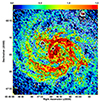 |
Fig. 2. LOFAR radio continuum map of IC 342 observed at 0.144 MHz overlaid with contours of the VLA 1.4 GHz emission. Contour levels are 3, 6, 12, 24, 32, 10−4 Jy/beam. Dashed circles indicate the positions of the background radio sources that were subtracted for this study. The beam size of 10.5″ is indicated in the bottom-left corner of the image. |
About 56% of the low-frequency radio sources were identified as star-forming regions through cross-matching with 22 μm emitting sources. The rest could be background radio source candidates, particularly those in the inner R < 7 kpc disk. Identifying the origin of the radio sources beyond R ∼ 7 kpc is not as straightforward because the 22 μm emission is mainly limited to the inner disk. Studying the radio–FIR correlation, we subtracted known background radio sources. For instance, the bright unresolved source located northeast of the nucleus (α = 3h 47m 29s, δ = 68° 08′ 24″) was omitted. Turner & Ho (1983) identified this source as having a distinct double-lobed appearance typical of a radio galaxy, with a 21 cm continuum flux of 46 mJy. Furthermore, Hummel (1991) confirmed this identification, noting a steep spectral index of α = −0.87, consistent with that of a background radio galaxy. Similarly, the unresolved source positioned near the edge of the primary beam to the northwest (α = 3h 45m 23s, δ = 68° 17′ 00″), with a 21 cm continuum flux of 26 mJy was also identified as a background galaxy by Hummel (1991). The likelihood of this source being within IC 342 is minimal, as its total-power output exceeds that of Cas A by a factor of six, which is uncharacteristic for sources within the galaxy (Crosthwaite et al. 2000). Two other radio sources at α = 3h 47m 14s, δ = 68° 05′ 10″ and α = 3h 46m 54s, δ = 68° 06′ 5″ were also excluded. They are likely external sources, as they were detected only at 0.14 GHz and lack counterparts in the IR and FUV maps.
4. Thermal and nonthermal radio maps
As discussed in Sect. 1, to investigate the origin of the resolved radio–FIR correlation and to assess the role of the magnetic fields and CREs, the thermal and nonthermal components of the radio continuum emission should be separated. This also helps map the pure nonthermal spectral index that is proportional to the energy index of CREs in order to address their cooling across the galaxy. Although, globally, the thermal emission represents no more than 10% at 1.4 GHz and about 5% at 0.33 GHz (Basu et al. 2012; Tabatabaei et al. 2017), it can be larger than 20−30% in star-forming regions (Tabatabaei et al. 2022), even at low frequencies (Hassani et al. 2022). Hence, we mapped the thermal and nonthermal emission at all radio frequencies of study.
We needed a separation method with no prior assumption about the nonthermal spectral index. In an ionized gas, ideal tracers of the free-free emission are recombination lines with Hα emission as the brightest indicator. Using a de-reddened Hα map has been the most feasible technique to study the thermal and nonthermal emission from different galactic regions (e.g., arms versus inter-arm regions, inner versus outer disks) down to very low surface brightness levels (Tabatabaei et al. 2007a, 2013a,b, 2017, 2022; Hassani et al. 2022; Heesen et al. 2022). To our knowledge, IC 342 lacks a complete and reliably calibrated Hα map, which can be because of its low-declination (viewed through the Milky Way disk) and low-surface brightness. Therefore, we had to use another thermal tracer for this galaxy. Several studies have explored the use of the mid-IR emission at 22−24 μm wavelength to estimate the thermal free-free flux density (e.g., Murphy et al. 2006a; Basu et al. 2012). These studies show that, as an SFR tracer, the mid-IR emission can also provide an accurate free-free template in star-forming regions. For IC 342, we opted to use the WISE 22 μm data to map the thermal radio emission. Following Murphy et al. (2006a), the radio thermal emission flux density,  , in Jansky (per pixel) is related to the 24 μm flux, f24, as
 (1)
(1)
where ν is the radio frequency and T is the thermal electron temperature, which is typically 104 K. After convolving the maps to the same resolution and normalizing them to the same pixel size and geometry, we first obtained the thermal radio flux densities per pixel using Eq. (1). The nonthermal emission was then computed for each pixel by subtracting the thermal flux from the observed radio continuum flux at each frequency ( ). Figure 3 shows the resulting maps of the thermal and nonthermal emission. The nonthermal maps exhibit a pronounced large-scale spiral pattern unlike the thermal maps, although both are brighter in the center and star-forming regions. The two background radio sources, one near the center of the galaxy at a distance of 2.4 kpc (RA = 3h 47m 27s and Dec = 68° 8′ 17″) and the other at a distance of 6.3 kpc from the center in the northeast of the galaxy (RA = 3h 45m 19s and Dec = 68° 16′ 23″), are the brightest sources in the nonthermal map.
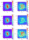 |
Fig. 3. Maps of the thermal (left) and nonthermal synchrotron (right) radio continuum emission from IC 342 at the 4.8 GHz (top row), 1.4 GHz (middle row), and 0.144 GHz (bottom row) frequencies, all at a 25″ angular resolution. Color bars show the intensities in units of Jansky per pixel. |
Obtaining the thermal fraction defined as  provides more detailed insights into the relative contributions of the thermal and nonthermal processes across the galaxy. We calculated the thermal fraction for the entire galaxy and for two different regimes of star-forming ISM, separately. We utilized the 22 μm map to delineate a densely star-forming regime (R1) and a diffuse and weakly star-forming regime (R2), as explained in Appendix A. At 144 MHz, the thermal fraction in R1 and R2 are 5.7%±0.5 and 1.1%±0.1, respectively, increasing to 13.5%±1.0 and 3.5%±0.3 at 1.4 GHz. At 4.8 GHz, the thermal fraction reaches 29.7%±2.1 and 8.7%±0.6 in R1 and R2, respectively. These systematic variations demonstrate that the thermal processes are more tied to massive star formation dominating in the spiral arms than in diffuse ISM. On average, the nonthermal emission dominates the thermal emission in both R1 and R2, even at 4.8 GHz in IC 342. At all three frequencies investigated (4.8 GHz, 1.4 GHz, and 0.144 GHz), the highest thermal fraction is consistently observed in the central region of the galaxy, with a fraction of 63%±4.7, 35%±2.5, and 20%±1.6, respectively, due to its high SFR activity and dense ionized gas. Table 3 lists the integrated flux densities and thermal fractions for the entire galaxy and R1 and R2. The reported values for the entire galaxy were obtained by integrating the observed and thermal RC maps in the plane of the galaxy (i = 31°) around the center out to a radius of R < 10 kpc.
Radio continuum flux densities and thermal fractions of IC 342 and its regions.
5. Synchrotron spectral index
The nonthermal radio maps derived in Sect. 4 were used to obtain the synchrotron spectral index (α, S ∝ να) over the entire frequency range of 0.14 to 4.8 GHz, α[0.1 − 4.8], at a 25″ angular resolution (Fig. 4). This was obtained only for pixels with intensities above 3σ rms noise levels. We find that the spectral index changes across the disk. It is flatter in star-forming regions in the galaxy center and in the spiral arms than in other places in the galaxy. The distribution of the synchrotron spectrum across the disk agrees with the injection of CREs into star-forming regions and their energy loss propagating away from these regions toward the inter-arm and outer disk. This agrees with previous findings in other nearby galaxies such as M 33 and NGC 6946 (Tabatabaei et al. 2007a, 2013a, 2022; Hassani et al. 2022). The median value of α[0.1 − 4.8] across IC 342 is −0.70 with a dispersion of 0.06, as shown in the histogram representation (Fig. 5). This is flatter than the typical synchrotron spectral index found for galaxies in the mid-radio frequencies of 1−10 GHz (≃ − 0.97 ± 0.16, Tabatabaei et al. 2017). To be more certain about the flattening, we derived the spectral index separately for two frequency intervals lower and higher than 1.4 GHz (i.e., α[0.1 − 1.4] and α[1.4 − 4.8]). Figure 5 shows that the spectral index is on average flatter in the low-frequency interval (α[0.1 − 1.4] = −0.51 ± 0.09) than in the high-frequency interval (α[1.4 − 4.8] = −1.06 ± 0.19). Thus, while the spectral index agrees with that of Tabatabaei et al. (2017) at the high-frequency interval, it becomes flatter at low frequencies ν < 1.4 GHz. A similar flattening has been reported for other LoTSS galaxies by Heesen et al. (2022). It is important to note that this low-frequency flattening occurs not only in star-forming regions but also in more diffuse parts of the ISM (Fig. 4).
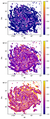 |
Fig. 4. Synchrotron spectral index maps of IC 342 for α[1.4 − 4.8] (top), α[0.14 − 4.8] (middle), and α[0.14 − 1.4] (bottom) overlaid with contours of the 22 μm emission indicating star-forming regions. Contour levels are 2, 4, 6, 8, and 10 × 10−4 Jy/pix. |
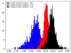 |
Fig. 5. Histogram of the synchrotron spectral index in the high-frequency interval of 1.4 ≤ ν ≤ 4.8 GHz (blue), the entire frequency interval of 0.14 ≤ ν ≤ 4.8 GHz (red), and low-frequency interval of 0.14 ≤ ν ≤ 1.4 GHz (black). |
6. Magnetic field strength
The strength of the total magnetic field Btot is related to the nonthermal synchrotron In intensity. Assuming that the energy densities of the magnetic field and cosmic rays are equal  :
:
![Mathematical equation: $$ \begin{aligned} B_{\rm tot} = C(\alpha _{n},K,L)[I_{n}]^{\dfrac{1}{\alpha _{n}+3}}, \end{aligned} $$](/articles/aa/full_html/2024/11/aa51110-24/aa51110-24-eq6.gif) (2)
(2)
where C is a function of the synchrotron spectral index αn, K is the ratio between the number densities of cosmic ray protons and electrons, and L is the path length in the synchrotron-emitting medium (see Beck & Krause 2005). Assuming that the magnetic field is parallel to the plane of the galaxy (inclination of i = 31° and position angle of the major axis of PA = 39°), Btot is mapped across the galaxy using the nonthermal emission at 1.4 GHz and αn = α[1.4 − 4.8], which is close to the theoretical synchrotron loss spectral index. The usage of the low-frequency part of the spectrum (ν < 1.4 GHz) in Eq. (2) can lead to an incorrect result because the low-frequency flattening (Sect. 5) can be linked to unrelated energy loss mechanisms or absorption effects. In our calculations, we used K ≃ 100 (Beck & Krause 2005) and L ≃ 1 kpc/cos(i).
Figure 6 shows that the magnetic field is strongest in the center of the galaxy (Btot ≃ 20 μG), while it is ≃10 μG in other star-forming regions and spiral arms. On average, we find that Btot = 10.23 ± 1.30 μG over the disk of IC 342, which is about 20% weaker than what was obtained by Beck (2015). This discrepancy can be attributed to the utilization of distinct methodologies for separating the thermal and nonthermal emission. Notably, our approach refrains from relying on any a priori assumptions regarding the nonthermal spectral index.
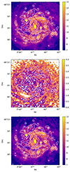 |
Fig. 6. Magnetic field strength maps in IC 342. Strength of the total magnetic field Btot obtained using the synchrotron emission at 1.4 GHz in IC 342 at a 25″ angular resolution (top). Also shown are maps of the ordered Bord (middle) and turbulent Btur (bottom) magnetic field strengths. The bars on the right of each image show the magnetic field strength in μG. Contours show the 22 μm emission at levels of 2, 4, 6, 8, and 10 × 10−4 Jy/pix. |
As the fraction of the polarized intensity (PI) is related to the strength of the ordered magnetic field and the nonthermal intensity In to the total magnetic field in the plane of the sky, In − (PI/0.75) gives the nonthermal emission due to the turbulent magnetic field Btur (Tabatabaei et al. 2008). Using this intensity in Eq. (2) yields the distribution of Btur across the galaxy. We also mapped the strength of the ordered magnetic field defined as Bord2 = Btot2 − Btur2. As shown in Fig. 6, the ordered field is stronger in the outer disk than in the inner disk. We inferred that the strong Btot in star-forming regions is mainly due to turbulence, as Btur is also stronger there. It is also likely that in star-forming regions, the ordered field has different directions (or tangled), and their polarization signals cancel each other out within the beam size. As such, the structure of Btur can be a combination of a random isotropic component and a field tangled on unresolved scales. In other words, we cannot distinguish between unresolved structures of the ordered field and truly turbulent fields for structures smaller than the beam.
7. Radio–FIR correlation
When investigating the nonthermal radio–FIR correlation, we invoked various approaches often used in resolved studies: the classical pixel-wise correlation, the FIR-to-radio ratio mapping, and multi-scale analysis. We performed the first two approaches at all three radio frequencies at a 25″ angular resolution (that of the 4.8 GHz). As a higher resolution is preferred for the multi-scale analysis, the method uses only the 0.14 and 1.4 GHz maps at a 15″ (≃0.2 kpc) resolution. The Herschel PACS FIR data are used at different bands of 70, 100, and 160 μm to investigate the possible influence of dust temperature (warmer dust is traced at a shorter FIR wavelength). These approaches and their results are presented as follows.
7.1. Pixel-by-pixel correlation
The Pearson’s linear correlation coefficient between two images of identical pixels i, S1(x, y) and S2(x, y), is given by
 (3)
(3)
where S1i and S2i represent the intensity of the i-th pixel in images one and two, respectively. The mean of the pixel intensity values in each image is denoted as  and
and  , with n as the total number of pixels.
In the case of a perfect correlation, rp = 1; and for a perfect anticorrelation, rp = −1. If the two images are completely uncorrelated, then rp = 0. The statistical error in rp is given by  , which depends on the strength of the correlation and the number of pixels, n.
To extend the analysis, Pearson correlation coefficients were computed for the radio continuum and FIR bands at 70, 100, and 160 μm, focusing on regions delineated as R1 (star forming) and R2 (diffuse), as discussed in Sect. 4. Sets of independent data points (n) were established, ensuring a beam area overlap of less than 20% and selecting pixels spaced by more than one beamwidth. A Student’s t-test was subsequently applied to assess the statistical significance of the correlations. It is noteworthy that both the observed radio continuum maps at 1.4 GHz and 4.8 GHz, as well as their synchrotron components, exhibit strong correlations with the FIR maps, particularly within the star-forming regime (R1), with correlation coefficients (rp) exceeding ≈0.90 (Table 4). Conversely, in the diffuse regime (R2), correlations are weak, typically below rp ≈ 0.5. This underscores the variability in the strength of the radio–FIR correlations across different environments within the galaxy. For the entire galaxy, the correlations at 0.144 GHz are not as tight as those at higher frequencies (rp ≲ 0.70). However, the correlations are much improved in the R1 regime (i.e., in denser parts of the ISM). This shows the significance of the diffuse component at 0.144 GHz causing the relatively weak radio–FIR correlation for the entire galaxy.
Radio–FIR break scales (lbreak) in kiloparsecs.
It is interesting to note that the correlations at different FIR bands all agree within the errors irrespective of the region. This indicates that dust temperature does not play a role in this correlation in IC 342 unlike in M 33 (Tabatabaei et al. 2007a,b). It is likely that the warm and cold dust components are well mixed or that the radiation field does not change much across the galaxy. The fact that this galaxy does not host giant HII complexes such as those in M 33 producing energetic ionizing UV photons means that dust is heated mainly by an almost uniform interstellar radiation field, at least down to the resolution of this study (≃200 pc).
We note that almost all correlations follow a sub-linear radio versus FIR relation (or a super-linear FIR versus radio). For example, the synchrotron emission at 1.4 GHz is correlated with the FIR emission at 70 μm with a slope of 0.79 ± 0.03 (in the log–log plane) with a t-test value large enough to be taken as statistically significant (t > 2). A similar sub-linearity between the radio continuum emission and different SFR tracers was reported in other resolved studies (e.g., Heesen et al. 2014) and is linked to diffusion of CREs (e.g., Berkhuijsen et al. 2013).
7.2. FIR-to-radio ratio map
As already shown in the pixel-by-pixel correlation analysis, the radio-FIR correlation changes depending on the level of star formation activity in IC 342. Another method to assess the relative variations of the radio and FIR emission locally is to map the ratio of the FIR to radio fluxes in logarithmic scale (called as q-parameter, see e.g., Murphy et al. 2006b; Hughes et al. 2006; Tabatabaei et al. 2013b). This will further help investigate if variations in the radio–FIR correlation correspond to particular physical structures in IC 342. When calculating the q-parameter, it is common to use a combination of the IRAS bands at 60 μm and 100 μm as a proxy of the integrated FIR emission in the frequency range of 42−122 μm (Helou et al. 1988), a single IR band at 24 μm or 70 μm (Appleton et al. 2004; Murphy et al. 2006b), or direct integration of the IR SEDs (Tabatabaei et al. 2013b, 2017). In this study, considering the available data1, we opted to use the single-band 70 μm data to map the q-parameter following the convention by Appleton et al. (2004) and Murphy et al. (2006b):
 (4)
(4)
In this definition, Sradio is the radio flux density, and S70 μm is the monochromatic 70 μm flux density. We obtained the q-parameter for the nonthermal synchrotron emission (as Sradio in Eq. (4)) at the conventional radio frequency of 1.4 GHz (q1.4). For comparison, we also mapped this quantity at the low radio frequency of 0.14 GHz (q0.1). The maps are constructed excluding pixels below the 3σ rms noise level in the synchrotron and FIR maps. As shown in Fig. 7, the q-parameter is generally higher in the spiral arms and star-forming regions irrespective of the radio frequency, in agreement with Tabatabaei et al. (2013b). Figure 8 also presents a histogram of q1.4 and q0.1 in the star-forming regime (R1) in IC 342. On average, q = 2.16 ± 0.23 using the 1.4 GHz synchrotron emission, which agrees with previous studies. A lower value was obtained using the radio synchrotron emission at a lower frequency of 0.144 GHz (q = 1.68 ± 0.28), consistent with Yun et al. (2001) and Read et al. (2018), while it is higher when using the 4.8 GHz emission (q = 2.73 ± 0.22).
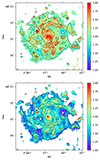 |
Fig. 7. Logarithmic ratio of the 70 μm emission to the radio synchrotron intensity at 1.4 GHz (q1.4, top) and 0.14 GHz (q0.14, bottom) at a 25″ angular resolution. Contours show the 22 μm emission at levels of 2, 4, 6, 8, and 10 × 10−4 Jy/pix. |
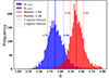 |
Fig. 8. Histogram of q1.4 (red) and q0.14 (blue) in star-forming regime of the ISM (R1) in IC 342. The median value of each distribution (solid lines) and their 1-sigma intervals (solid lines) are also indicated. |
7.3. Multi-scale correlation
The pixel-by-pixel correlation can be biased toward a specific scale if its corresponding structure contains relatively more weight (brightness) in a map. Hence, we also used a scale-by-scale analysis by means of a 2D Wavelet decomposition that consists of the convolution of an image with a set of self-similar basis functions that vary with scale and location. In general, the wavelet transform can be understood as a generalization of the Fourier transform. The oscillatory function is both localized in time and in frequency in the wavelet transform. Based on a mother function, called the analyzing wavelet, the family of basis functions is generated. Throughout this paper, we employ the continuous wavelet transform in two dimensions:
 (5)
(5)
A wavelet is a multidimensional function representing the position of a wavelet, where f(x) is a two-dimensional function (an image), ψ(x) is the analyzing wavelet, the symbol * is the complex conjugate, x = (x, y) represents the position, and a indicates its scale. An energy normalization parameter, κ, was applied (we used κ = 2). Following Frick et al. (2001), to achieve both good spatial and scale resolution, we used the “PetHat” function as the processing wavelet ψ(x). For two identical images with the same size and linear resolution, the wavelet cross-correlation coefficient at scale a is defined as follows:
![Mathematical equation: $$ \begin{aligned} r_{{ w}}(a) = \dfrac{\int \int W_{1}(a,x)\,W^{*}_{2}(a,x)\,\mathrm{d}x}{[M_{1}(a)\,M_{2}(a)]^{1/2}}, \end{aligned} $$](/articles/aa/full_html/2024/11/aa51110-24/aa51110-24-eq13.gif) (6)
(6)
with  , the wavelet equivalent of the power spectrum in Fourier space. The value of rw varies between −1 (total anticorrelation) and +1 (total correlation). In the case of a given scale, a correlation coefficient of |rw| = 0.5 represents a marginal value for accepting the correlation between the structures (Tabatabaei et al. 2013a). The error in rw is given by
  , with n as the number of points at each specific scale.
We decomposed all the radio and FIR maps into 50 angular scales between 7″ ∼ 111 pc (half of the beam width, following Frick et al. 2001) and 1007″ ∼ 16 kpc to a map with one-third the image size in order to avoid boundary effects. Then the wavelet coefficients W(a, x) of the radio and FIR maps were driven and used in Eq. (6) to calculate the wavelet correlation coefficient rw for every scale of decomposition.
Figure 9 shows the wavelet correlation coefficients rw versus scale for each pair of the radio (at 0.14 and 1.4 GHz) and FIR bands at 70, 100, 160 μm. As rw = 0.5 indicates the same number of correlated and uncorrelated structures in two decomposed maps, we considered this coefficient as a marginal condition for the acceptance of a correlation between the structures following Tabatabaei et al. (2013a). At each FIR band shown in Fig. 9, a general dropping trend was found for the correlations from large to small scales. When defining the smallest scale of the correlation (i.e., where rw = 0.5 is the break scale, lbreak), we found that both the observed and the nonthermal radio continuum emission at 1.4 GHz are correlated with the FIR emission on scales ≥180 − 200 pc (=lbreak, 1.4). At the lower radio frequency of 0.14 GHz, a similar large-to-small-scale dropping trend exists; however, the break scale occurs on scales of ≥0.28 − 0.36 pc (=lbreak, 0.14), that is, larger than those at 1.4 GHz. Therefore, a scale difference was found for the correlation depending on the radio frequency. Supposedly, lower radio frequencies trace older and more diffused CREs. Hence, a larger break scale at lower frequencies shows that a fine balance between gas, CREs and the magnetic field is indeed the most fundamental requirement for the radio-FIR correlation to be held (Tabatabaei et al. 2013a). It is also instructive to note that CREs traced at 0.14 GHz are propagated away on a path length about twice as long as those traced at 1.4 GHz (lbreak, 0.14 ≃ 1.8 lbreak, 1.4). These findings are discussed further in Sect. 8. By comparing different FIR bands shown in different panels in Fig. 9, we found that the correlations are almost similar at 1.4 GHz, while a larger scatter in lbreak was found at 0.14 GHz. Additionally, it should be mentioned that the break scales determined with the smoothing method (Heesen 2021; Vollmer et al. 2020) are larger than the values of the radio–FIR break scales given in Table 42.
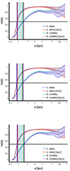 |
Fig. 9. Multi-scale correlation between the radio continuum emission and the FIR bands at 70 μm (top), 100 μm (middle), and 160 μm (bottom). In each panel, the solid horizontal line shows rw = 0.5, and vertical lines indicate its corresponding scales of occurrence (lbreak) for different radio and FIR pairs. |
8. Discussion
In the following, we discuss the variations in the radio–FIR correlation in the disk of IC 342 and investigate the role of the propagation of CREs in this correlation. Then, possible CRE cooling mechanisms, diffusion, and their related timescales are investigated and compared with other galaxies.
8.1. Sources of variation in the radio-FIR correlation
The radio–FIR correlation assessed via the FIR-to-radio ratio (q) is often used to calibrate the SFR globally in galaxy samples because it does not change systematically with the SFR itself in star-forming galaxies (Yun et al. 2001). However, q can change locally inside galaxies, as shown in a sample of the SINGS galaxies (Murphy et al. 2008), NGC 6946 (Tabatabaei et al. 2013b), the LMC (Hughes et al. 2006), and in IC 342 (Sect. 7.2). A first possible reason for a change in q can be different origins of the nonthermal radio and thermal FIR emission in some locations in a galaxy. For instance, we can refer to diffuse parts of the ISM where the FIR emission can be due to dust heated by non-ionizing photons from old solar-mass stars, while the synchrotron radiation is generated by secondary CREs propagated away in the ISM. In this case, no radio–FIR correlation is in fact expected. Accordingly, we can explain the maximum dispersion from the mean value of q (< 2) in IC 342 as it occurs in R2, where indeed no correlation holds (Sect. 7.1). On the other hand, smaller variations are even found in the star-forming regime R1. Although the correlation holds tightly, q still changes locally there. In this case, a common source (e.g., massive stars) can be responsible for both the nonthermal radio and the thermal FIR emission but following different dependencies. We investigated this further by focusing on the R1 regime.
We first derived the star formation surface density (ΣSFR) using a combination of the FUV and mid-infrared (MIR) emission presented by Bigiel et al. (2008) as a hybrid tracer,
 (7)
(7)
In the above calibration relation, the intensity of the MIR (22 μm) emission is used as a proxy for the extinction of the FUV emission. In Fig. 10, the FIR-to-synchrotron ratio at 1.4 GHz (q1.4) and 0.14 GHz (q0.14) is plotted against ΣSFR taking into account only pixels above a 3σ rms noise level. With a Pearson correlation coefficient of ≃0.7 (0.6), q increases with ΣSFR as
 (8)
(8)
and
 (9)
(9)
at 1.4 GHz and 0.14 GHz, respectively. A tight positive correlation was also found in NGC 6946, although with a much flatter slope of ≃0.1 (Tabatabaei et al. 2013b). Assuming that the FIR emission (here the 70 μm emission) is linearly correlated with the SFR, this increase must be due to a sub-linear correlation of the synchrotron emission and SFR. As shown in Fig. 11, this is exactly what occurs in the star-forming ISM (R1) of IC 342. This means that the synchrotron emission is not produced as efficiently as the FIR emission with SFR. However, as shown in Fig. 6, it is expected that the magnetic field becomes stronger in star-forming regions, which should result in the synchrotron cooling of CREs via the synchrotron radiation. The nonefficient synchrotron emission observed in the star-forming regions has two main possible causes: (1) a non-efficient amplification of the magnetic field and (2) decoupling and escape of the CREs via winds in these regions (Tabatabaei et al. 2022). These reasons are addressed in Sects. 8.2 and 8.3.
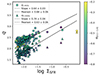 |
Fig. 10. Logarithmic ratio of the 70 μm to the radio synchrotron emission at 1.4 GHz (q1.4, circles) and 0.14 GHz (q0.14, triangles) versus star formation surface density ΣSFR (M⊙ yr−1 kpc−2) in regime R1. Solid lines show bisector OLS fits. The color bar shows the spectral index between 0.14 and 1.4 GHz α[0.1 − 1.4]. |
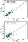 |
Fig. 11. FIR emission at 70 μm (top) and synchrotron emission at 1.4 GHz (bottom) versus SFR surface density ΣSFR (M⊙ yr−1 kpc−2) in the star-forming regime (R1). Solid lines show bisector OLS fits. |
8.2. Magnetic field and star formation
As mentioned in Sect. 8.1, the magnetic field is expected to be amplified due to star formation activities. One of the most important mechanisms often considered is supernova-driven turbulence (Gressel et al. 2008). The energy density of the turbulent gas motions is then converted to the magnetic energy density by a small-scale dynamo mechanism. This leads to a power-law relation between the magnetic field strength and SFR surface density with an index of 0.3 ( ), assuming equipartition between the magnetic field and cosmic rays (Schleicher & Beck 2013). We investigated whether such a correlation holds in IC 342. The equipartition magnetic field strength obtained using the 1.4 GHz synchrotron emission (Sect. 6) shows a modest correlation with ΣSFR, with a Pearson correlation coefficient of ≃0.55 for both total and turbulent fields (Fig. 12). For the entire galaxy, the correlation between the total magnetic field strength and ΣSFR can best be explained by the following power-law relationship obtained using OLS bisector regression:
 (10)
(10)
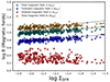 |
Fig. 12. Total, turbulent, and ordered magnetic field strength obtained using the synchrotron emission at 1.4 GHz (circles) and 0.14 GHz (triangles) versus SFR surface density ΣSFR (M⊙ yr−1 kpc−2). Solid lines show bisector OLS fits. For better visualization, the turbulent magnetic field strength has been shifted by 0.2 along the y-axis. |
The same relation is obtained between the turbulent field and SFR surface density. The ordered field shows a decreasing trend with ΣSFR but with a large scatter (rp = −0.3). This is expected because the field becomes more turbulent or tangled in the star-forming regions. Table 5 summarizes rp and the fit power-law exponents we obtained.
Correlation coefficients and power-law exponents for magnetic field strengths.
As noted by Hassani et al. (2022) and Tabatabaei et al. (2022), the slope of the Btot − ΣSFR relation can be flat due to contamination by the diffuse ISM. When focusing on the star-forming regime R1, we obtained
 (11)
(11)
which is slightly steeper than what is given in Eq. (10). We note that the same correlation and power-low exponent is obtained if the low-frequency synchrotron emission at 0.14 GHz is used to estimate the magnetic field strength.
Compared with similar studies in other nearby galaxies, the B–SFR correlations are generally weaker in IC 342. The exponents obtained for the entire galaxy agree with those derived in NGC 6946 (0.14 ± 0.01, Tabatabaei et al. 2013b) and NGC 4254 (0.18 ± 0.01, Chyży 2008) within uncertainties but are flatter than those in the LMC and SMC (≃0.25 − 0.30, Hassani et al. 2022, which is closer to the theoretical small-scale dynamo value), perhaps due to intervening amplification mechanisms such as gas compression in the ISM of spiral galaxies, which is denser than that in dwarf irregulars.
8.3. Effect of star formation and magnetic field on the energy spectrum of CREs
The energy of CREs follows a power-law distribution of the form Eν ∝ νp, with p = (2α − 1) as the energy index and α as the radiation spectral index (Sν ∝ να). Theoretically, CREs are injected with a flat power-law index of p = −2 or a spectral index of α = −0.5 from their sources in star-forming regions (e.g., SNRs). As they propagate away, they can lose their energy as a result of interaction with matter (via ionization or adiabatic losses), magnetic fields (via synchrotron loss), and radiation (via inverse Compton loss). Hence, the spectral index maps presented in Fig. 4 can be used to infer the locations in the galaxy where CREs gain or lose energy and to further study the role of the SFR and magnetic fields.
Theoretically, the energy spectrum of cosmic rays can be affected by both massive star formation activity (a flattening or energy gain) and magnetic fields (a steepening or energy loss) in an opposite way. Observations in other galaxies have already confirmed the expected trend with ΣSFR (i.e., flattening of the spectral index). However, in spite of a steeper α along the ordered magnetic field observed in NGC 6946 (Tabatabaei et al. 2013b), no clear trend with the total magnetic field strength is reported in the literature. In fact, separating the two effects can be difficult if the magnetic field is also amplified and generated in star-forming regions, which is often the case (Tabatabaei et al. 2020). These effects are revisited in IC 342. Figure 13 shows the spectral index versus ΣSFR and Btot. Table 6 lists the corresponding correlation coefficients rp and the fitted power-law exponents for the case of a reasonable correlation (rp > 0.30). Remarkably, the analysis revealed a distinct correlation between ΣSFR and the spectral index measured between 4.8 GHz and the other two frequencies, α[1.4 − 4.8] and α[0.1 − 4.8]. This correlation suggests a potential influence of massive star formation activity on the energy spectrum of cosmic rays in IC 342, akin to observations in other galaxies (e.g., Tabatabaei et al. 2013b, 2022). The flattening of the spectral index with increasing ΣSFR underscores the significance of star-forming regions in shaping the spectrum of CREs traced at higher frequencies. In the low-frequency domain (between 0.1 and 1.4 GHz), the synchrotron spectrum is flat regardless of the level of star formation, and therefore the correlation of α[0.1 − 1.4] with ΣSFR is weak (rp = 0.21 ± 0.02). The flattening of the spectrum at low frequencies can be caused by absorption effects in cool ionized gas (Israel & Mahoney 1990; Israel et al. 1992) or efficient ionization loss of CREs (Hummel 1991).
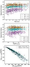 |
Fig. 13. Synchrotron spectral index and its relationship with star formation and magnetic field strength. Top: Synchrotron spectral index obtained at different frequency intervals (α[0.1 − 1.4], α[1.4 − 4.8] and α[0.1 − 4.8]) versus star formation surface density ΣSFR (M⊙ yr−1 kpc−2). Lines show bisector OLS fits. Middle: Same spectral indices versus the total magnetic field strength. Bottom: Synchrotron spectral index α[1.4 − 4.8] versus magnetic field after compensating both for the effect of the SFR. |
Correlation coefficients and power-law exponents for spectral indices.
Unlike with ΣSFR, the correlations with Btot are less straightforward. Contrary to expectations based on the effects of magnetic fields, there is no discernible correlation between Btot and the spectral index across the observed data points (rp ≤ 0.3). The increase of both α and Btot in star-forming regions can reduce the expected steepening of the synchrotron spectrum with increasing magnetic field strength (here, an α − Btot anticorrelation). To compensate for the effect of star formation, we investigated their correlation after normalizing them to ΣSFR. The bottom panel in Fig. 13 shows that per unit ΣSFR, a tight linear anticorrelation holds between the spectral index and total magnetic field strength. Hence, our observations in IC 342 confirm the theoretical expectation for synchrotron cooling of CREs based on the steepening of the synchrotron spectrum per unit ΣSFR.
8.4. Propagation of CREs
The degree of order of the magnetic field is believed to play a significant role in theoretical models of the propagation of CREs (i.e., the streaming instability models Kulsrud 2005; Enßlin et al. 2011, and diffusion models Ptuskin et al. 1993; Breitschwerdt et al. 2002; Dogiel & Breitschwerdt 2012; Shalchi et al. 2009). Apart from streaming and diffusion, the escape of CREs can affect their propagation, as discussed by Helou & Bicay (1993) and Heesen (2021) for example.
As a result of streaming, CREs move along the lines of the ordered field at the Alfvén velocity (υA) and propagate over a distance of lprop = υA tCRE during their lifetime (tCRE). Basically, streaming requires long stretches of the ordered field to be effective. Hence, it may not be important in the turbulent thin disk of galaxies. On the other hand, studies of the Milky Way have shown that the propagation of CREs is isotropic on scales < 1 kpc (Strong et al. 2007; Tsap et al. 2012), which is not in accordance with streaming. Accordingly, it is assumed that diffusion dominates streaming except in regions with highly ordered fields, where streaming may dominate.
Diffusion occurs when irregularities in the turbulent magnetic field scatter the particles. The diffusion length is theoretically defined as ldif = 2 (D tCRe)0.5, with D as the diffusion coefficient and tCRe as the lifetime of CREs. The diffusion of CREs in the ISM has been described as
 (12)
(12)
by Ptuskin et al. (1993), Breitschwerdt et al. (2002), Yan & Lazarian (2004), Dogiel & Breitschwerdt (2012), and Shalchi et al. (2009). Assuming that the lifetime of CREs is limited by the synchrotron loss during the synchrotron timescale,  , we can derive the CRE diffusion length as
 (13)
(13)
On the other hand, when taking into account the escape of CREs, the diffusion length of CREs can deviate from that given by Eq. (13). This is because the lifetime of a CRE is not primarily determined by synchrotron loss but rather by the escape from the disk (tCRE = tesc). Following Heesen et al. (2018), the escape time inversely correlates with the escape velocity ( ), which in turn increases with the SFR and, consequently, the total magnetic field strength,
  , approximately ∝Btot. In this case, the diffusion length is given by
 (14)
(14)
which is larger than that given by Eq. (13).
Tabatabaei et al. (2013a) proposed an observational method to estimate the propagation length of CREs based on the break in the synchrotron–FIR correlation. This was further strengthened by an observed increase of the break scale with both the ordered field and the degree of order of the magnetic field (i.e., the ordered-to-turbulent magnetic field, Bord/Btur, as expected from the theoretical models). In the following, we first derive ldif and D using this observational method in IC 342. Then, we compare the theoretical models with the observations in a sample of nearby galaxies, which is now larger than what was presented in Tabatabaei et al. (2013a). The results displaying the correlations based on the available data can be found in Figs. 14a and 14b.
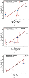 |
Fig. 14. Diffusion length of the CREs ldif obtained from observations versus what is expected from the theoretical diffusion model for the case of tCRE = tsyn (a, Eq. (13)) and tCRE = tesc (b, Eq. (14)). Also shown is the correlation of ldif with the ordered magnetic field (c). |
8.4.1. Diffusion length and coefficient of CREs in IC 342
As discussed in Sect. 7.3, the radio–FIR correlation to be held requires a fine pressure balance between CREs, magnetic fields and gas. Diffusion of CREs to large scales reduces their number density and violates the pressure balance on a scale that is equivalent to the diffusion length of CREs. Hence, the break scales in the synchrotron–FIR correlations obtained in Sect. 7.3 should be proportional to the diffusion length of CREs. As shown in Table 4, a noticeable difference in the break scale is found when using the radio emission at 1.4 GHz and 0.14 GHz. This can be explained by differences in the propagation of CREs traced across the frequency band. The synchrotron radiation at lower frequencies is generated by a lower energy (or older) population of CREs. This population must be the one already propagated to longer distances and has a longer diffusion length. Hence, depending on the frequency of the synchrotron emission, the CRE diffusion length is expected to vary.
Following the convention of Tabatabaei et al. (2013a), we used the break scale in the correlation between synchrotron emission and FIR emission at 70 μm (break occurs at a scale with rw ≤ 0.5) as the diffusion length of the CREs. For IC 342, we obtained a diffusion length of ldif, 1.4 = lbreak, 1.4 = 200 pc at 1.4 GHz. The diffusion length of CREs traced at a lower radio frequency of 0.14 GHz is larger (ldif, 0.14 = lbreak, 0.14 = 320 pc).
Assuming that the synchrotron and inverse Compton processes are the main sources of the energy loss of CREs (e.g., Condon 1992) and that tCRE = tsyn, these relativistic particles diffuse over a distance equivalent to their diffusion length, which is given by ldif = 2(D tsyn)0.5 before losing all of their energy to synchrotron and inverse Compton losses. Hence, taking into account that
 (15)
(15)
where
 (16)
(16)
the diffusion coefficient  can be estimated. For IC 342, by considering Btot ≃ 10 μg, we obtained tsyn ≃ 2.7 × 10⁷ years. Hence, D ≃ 1.1 × 1026 cm2 s−1 for CREs that emit at 1.4 GHz (
 = 200 pc). This is smaller than those assumed or estimated in other galaxies (D ≃ (1 − 10)×1028 cm2 s−1) based on theoretical (Roediger et al. 2007) or observational (Moskalenko & Strong 1998; Dahlem et al. 1995) studies. This implies that the assumption of tCRE = tsyn may not be correct in IC 342, and other processes, such as the escape of CREs, that lead to a larger ldif and D are needed.
8.4.2. Comparing with propagation models
The CRE propagation models we discussed can be tested in nearby galaxies if independent information about their ldif and magnetic field components is available. Similar multi-scale analysis of the radio–FIR correlation has been previously performed for a limited number of galaxies, namely M 31 and M 33 (Tabatabaei et al. 2013a), NGC 6946 (Tabatabaei et al. 2013b), M 51 (Dumas et al. 2011), the LMC (Hughes et al. 2006), and NGC 4214 (Howaida et al., in prep.). Table 7 lists the diffusion lengths of the galaxies along with their SFR and strengths of the magnetic field components. As the diffusion length for these galaxies is measured only at 1.4 GHz, we considered only ldif, 1.4 for IC 342 for the sake of consistency. Plotting ldif from observations versus what is expected from theory (Eqs. (13) and (14)) in Fig. 14, we found a roughly linear correlation for both cases of tCRE = tsyn and tCRE = tesc, although the scatter is smaller in the latter case, that is, when the escape of CREs is considered (Eq. (14)). We, however, found the tightest correlation between the observed ldif and the ordered magnetic field. A bisector OLS fit to the observed data resulted in
Magnetic field strengths and SFR surface density for nearby galaxies.
 (17)
(17)
This dependency can be explained if (i) the diffusion of CREs dominates along the ordered field with a diffusion coefficient of  (Shalchi 2009, Eq. (3.41)) or a length of
  and (ii) the CRE lifetime is given by a confinement time (i.e., the period that the CREs spend in the galactic disk) that is similar in different galaxies3, and (iii) Btur varies less than Bord between galaxies. In this case, we can show that
  , which is what is obtained in Eq. (17) observationally.
In Fig. 14c, NGC 6946 shows a deviation from the best-fit relation given in Eq. (17). As noted by Tabatabaei et al. (2013a), CRE streaming can dominate diffusion in this galaxy due to the presence of a large-scale ordered field, which is currently being amplified by a large-scale dynamo mechanism due to the disk-halo interaction (Beck 2007; Heald 2012). In case of streaming, lprop ∝ vA ∝ Bord, which is steeper than in Eq. (17). Moreover, ldif in NGC 6946 agrees with the diffusion length expected from synchrotron (tCRE ∼ tsyn, Tabatabaei et al. 2013b), unlike in IC 342 and likely other galaxies as well.
As explained in Sect. 6, part of the measured Btur can be due to the ordered magnetic field not detected in the polarization data because of the beam depolarization effects or mixing of several uniform field components with different directions along the line of sight. This can weaken the correlations with models that include Bord/Btur, such as those represented by Eqs. (13) and (14).
9. Summary and conclusion
This paper presents the LOFAR LoTSS observations of the radio continuum emission from the nearby galaxy IC 342 at 0.14 GHz. Combined with the archival radio data at 1.42 GHz and 4.85 GHz as well as the FIR Herschel observations at 70, 100, and 160 μm, we studied the radio-FIR correlation and its variation and dependencies on the SFR and ISM properties across the galactic disk. The radio-FIR correlation was calculated using the classical pixel-by-pixel correlation, the wavelet scale-by-scale correlation, and the q-method. Using WISE 22 μm maps, we corrected the radio synchrotron emission for thermal contamination. A de-reddened FUV map was used to trace the SFR in order to study its impact on the energy spectrum of the CREs. The strengths of the total, ordered, and turbulent magnetic fields were also mapped to evaluate their role in the radio–FIR correlation and cooling and propagation of CREs in this galaxy.
We find that the radio–FIR correlation is tight in star-forming regions. However, we also find a large scatter in the diffuse ISM of IC 342. This correlation is insensitive to the FIR bands, indicating that warm and cold dust components are well mixed or that the radiation field does not change much across this galaxy.
The sub-linear radio synchrotron versus FIR correlation and the variation in the FIR/radio ratio in star-forming regions shows that the synchrotron radiation is not produced as efficiently as the FIR emission despite the presence of a strong magnetic field in those regions. This indicates that besides the synchrotron cooling, CREs experience other processes, such as escape and diffusion. This is further confirmed by the multi-scale analysis of the correlation showing that the correlation breaks down on a scale that is proportional to the diffusion length of the CREs, which is set by the regularity of the magnetic field. We also show that the scale length of CREs decreases with radio frequency, as expected theoretically.
The cosmic ray energy spectrum can be affected by both massive star-formation activity (flattening or increased energy) and magnetic fields (steepening or reduced energy). Previous studies, however, had difficulty tracing and disentangling these two effects because the magnetic field strength increases with the SFR itself. Compensating for the effect of SFR, we find, for the first time, that the energy spectrum of CREs steepens with stronger magnetic fields and flattens with massive SFRs. Our study shows that the propagation of CREs in IC 342 is significantly influenced by the magnetic field structure. The diffusion length (ldif) represents the average distance CREs travel before scattering. The  indicates that the diffusion length increases with the magnetic field strength at a sublinear rate. Physically, this means that stronger magnetic fields enhance diffusion. This finding is crucial for predicting and managing diffusion processes in magnetic environments, providing a clear, quantifiable relationship between the field strength and diffusion length.
We note that the 22 μm IR data is used as a tracer of the free-free emission (and SFR); hence, it has not been utilized in calculating the q-parameter in order to avoid any artificial correlation when comparing it with ΣSFR in Sect. 8.1.
The magnitude of ldif relies on how the break scale is defined. For example, due to the strong correlation in the study of Mulcahy et al. (2014), they employed rw = 0.75 to establish the break scale. In this study, if we use rw = 0.75, we get average break scales of ∼260 pc for 1.4 GHz and ∼620 pc for 0.14 GHz.
As the scale height of the thin disk is about the same in these galaxies, the CREs need about the same time to diffuse out of the disk.
Acknowledgments
This paper is based (in part) on data obtained with the International LOFAR Telescope (ILT). LOFAR is the Low Frequency Array designed and constructed by ASTRON. It has observing, data processing, and data storage facilities in several countries that are owned by various parties (each with their own funding sources), and that are collectively operated by the ILT foundation under a joint scientific policy. The ILT resources have benefitted from the following recent major funding sources: CNRS-INSU, Observatoire de Paris and Université d’Orléans, France; BMBF, MIWF-NRW, MPG, Germany; Science Foundation Ireland (SFI), Department of Business, Enterprise and Innovation (DBEI), Ireland; NWO, The Netherlands; The Science and Technology Facilities Council, UK; Ministry of Science and Higher Education, Poland. MRC gratefully acknowledges the Canadian Institute for Theoretical Astrophysics (CITA) National Fellowship for partial support; this work was supported by the Natural Sciences and Engineering Research Council of Canada (NSERC). RJD acknowledges support by the BMBF Verbundforschung Projekt 05A23PC2.
References
- Appleton, P. N., Fadda, D. T., Marleau, F. R., et al. 2004, ApJS, 154, 147 [Google Scholar]
- Basu, A., Roy, S., & Mitra, D. 2012, ApJ, 756, 141 [NASA ADS] [CrossRef] [Google Scholar]
- Beck, R. 2007, A&A, 470, 539 [NASA ADS] [CrossRef] [EDP Sciences] [Google Scholar]
- Beck, R. 2015, A&A, 578, A93 [NASA ADS] [CrossRef] [EDP Sciences] [Google Scholar]
- Beck, R., & Krause, M. 2005, Astron. Nachr., 326, 414 [Google Scholar]
- Berkhuijsen, E. M., Beck, R., & Tabatabaei, F. S. 2013, MNRAS, 435, 1598 [Google Scholar]
- Bianchi, L. 2014, Ap&SS, 354, 103 [NASA ADS] [CrossRef] [Google Scholar]
- Bigiel, F., Leroy, A., Walter, F., et al. 2008, AJ, 136, 2846 [NASA ADS] [CrossRef] [Google Scholar]
- Blundell, K. M., & Rawlings, S. 2001, ApJ, 562, L5 [NASA ADS] [CrossRef] [Google Scholar]
- Breitschwerdt, D., Dogiel, V. A., & Völk, H. J. 2002, A&A, 385, 216 [NASA ADS] [CrossRef] [EDP Sciences] [Google Scholar]
- Calzetti, D., Wu, S.-Y., Hong, S., et al. 2010, ApJ, 714, 1256 [Google Scholar]
- Chyży, K. T. 2008, A&A, 482, 755 [NASA ADS] [CrossRef] [EDP Sciences] [Google Scholar]
- Clark, C. J. R., Verstocken, S., Bianchi, S., et al. 2018, A&A, 609, A37 [NASA ADS] [CrossRef] [EDP Sciences] [Google Scholar]
- Condon, J. J. 1992, ARA&A, 30, 575 [Google Scholar]
- Crosthwaite, L. P., Turner, J. L., & Ho, P. T. P. 2000, AJ, 119, 1720 [CrossRef] [Google Scholar]
- Crosthwaite, L. P., Turner, J. L., Hurt, R. L., et al. 2001, AJ, 122, 797 [NASA ADS] [CrossRef] [Google Scholar]
- Dahlem, M., Lisenfeld, U., & Golla, G. 1995, ApJ, 444, 119 [NASA ADS] [CrossRef] [Google Scholar]
- Davies, J. I., Baes, M., Bianchi, S., et al. 2017, PASP, 129, 044102 [NASA ADS] [CrossRef] [Google Scholar]
- de Jong, T., Klein, U., Wielebinski, R., & Wunderlich, E. 1985, A&A, 147, L6 [NASA ADS] [Google Scholar]
- de Vaucouleurs, G., de Vaucouleurs, A., Corwin, H. G., et al. 1991, Third Reference Catalogue of Bright Galaxies [Google Scholar]
- Dogiel, V. A., & Breitschwerdt, D. 2012, EAS Publ. Ser., 56, 61 [NASA ADS] [CrossRef] [EDP Sciences] [Google Scholar]
- Draine, B. T., Dale, D. A., Bendo, G., et al. 2007, ApJ, 663, 866 [NASA ADS] [CrossRef] [Google Scholar]
- Dumas, G., Schinnerer, E., Tabatabaei, F. S., et al. 2011, AJ, 141, 41 [NASA ADS] [CrossRef] [Google Scholar]
- Enßlin, T., Pfrommer, C., Miniati, F., & Subramanian, K. 2011, A&A, 527, A99 [Google Scholar]
- Fletcher, A., Beck, R., Shukurov, A., Berkhuijsen, E. M., & Horellou, C. 2011, MNRAS, 412, 2396 [CrossRef] [Google Scholar]
- Frick, P., Beck, R., Berkhuijsen, E. M., & Patrickeyev, I. 2001, MNRAS, 327, 1145 [CrossRef] [Google Scholar]
- Gavazzi, G., & Boselli, A. 1999, A&A, 343, 93 [NASA ADS] [Google Scholar]
- Graeve, R., & Beck, R. 1988, A&A, 192, 66 [NASA ADS] [Google Scholar]
- Gressel, O., Elstner, D., Ziegler, U., & Rüdiger, G. 2008, A&A, 486, L35 [NASA ADS] [CrossRef] [EDP Sciences] [Google Scholar]
- Gürkan, G., Hardcastle, M. J., Smith, D. J. B., et al. 2018, MNRAS, 475, 3010 [Google Scholar]
- Hassani, H., Tabatabaei, F., Hughes, A., et al. 2022, MNRAS, 510, 11 [Google Scholar]
- Heald, G. H. 2012, ApJ, 754, L35 [NASA ADS] [CrossRef] [Google Scholar]
- Heesen, V. 2021, Ap&SS, 366, 117 [NASA ADS] [CrossRef] [Google Scholar]
- Heesen, V., Brinks, E., Leroy, A. K., et al. 2014, AJ, 147, 103 [NASA ADS] [CrossRef] [Google Scholar]
- Heesen, V., Krause, M., Beck, R., et al. 2018, MNRAS, 476, 158 [CrossRef] [Google Scholar]
- Heesen, V., Staffehl, M., Basu, A., et al. 2022, A&A, 664, A83 [NASA ADS] [CrossRef] [EDP Sciences] [Google Scholar]
- Helou, G., & Bicay, M. D. 1993, ApJ, 415, 93 [Google Scholar]
- Helou, G., Soifer, B. T., & Rowan-Robinson, M. 1985, ApJ, 298, L7 [Google Scholar]
- Helou, G., Khan, I. R., Malek, L., & Boehmer, L. 1988, ApJS, 68, 151 [NASA ADS] [CrossRef] [Google Scholar]
- Hughes, A., Wong, T., Ekers, R., et al. 2006, MNRAS, 370, 363 [NASA ADS] [CrossRef] [Google Scholar]
- Hummel, E. 1991, A&A, 251, 442 [NASA ADS] [Google Scholar]
- Israel, F. P., & Mahoney, M. J. 1990, ApJ, 352, 30 [Google Scholar]
- Israel, F. P., Mahoney, M. J., & Howarth, N. 1992, A&A, 261, 47 [NASA ADS] [Google Scholar]
- Karachentsev, I. D., & Kashibadze, O. G. 2006, Astrophysics, 49, 3 [NASA ADS] [CrossRef] [Google Scholar]
- Karachentsev, I. D., Karachentseva, V. E., Huchtmeier, W. K., & Makarov, D. I. 2004, AJ, 127, 2031 [Google Scholar]
- Kennicutt, R. C., Calzetti, D., Aniano, G., et al. 2011, PASP, 123, 1347 [Google Scholar]
- Klöckner, H. R., Martínez-Sansigre, A., Rawlings, S., & Garrett, M. A. 2009, MNRAS, 398, 176 [CrossRef] [Google Scholar]
- Krause, M. 1990, Geophys. Astrophys. Fluid Dyn., 50, 43 [NASA ADS] [CrossRef] [Google Scholar]
- Krause, M. 1993, IAU Symp., 157, 305 [NASA ADS] [Google Scholar]
- Krause, M., Hummel, E., & Beck, R. 1989, A&A, 217, 4 [NASA ADS] [Google Scholar]
- Kulsrud, R. M. 2005, Plasma Physics for Astrophysics (Princeton: Princeton University Press) [Google Scholar]
- Leroy, A. K., Walter, F., Brinks, E., et al. 2008, AJ, 136, 2782 [Google Scholar]
- McCheyne, I., Oliver, S., Sargent, M., et al. 2022, A&A, 662, A100 [NASA ADS] [CrossRef] [EDP Sciences] [Google Scholar]
- Morrissey, P., Conrow, T., Barlow, T. A., et al. 2007, ApJS, 173, 682 [Google Scholar]
- Moskalenko, I. V., & Strong, A. W. 1998, ApJ, 493, 694 [NASA ADS] [CrossRef] [Google Scholar]
- Mulcahy, D. D., Horneffer, A., Beck, R., et al. 2014, A&A, 568, A74 [NASA ADS] [CrossRef] [EDP Sciences] [Google Scholar]
- Murphy, E. J., Helou, G., Braun, R., et al. 2006a, ApJ, 651, L111 [NASA ADS] [CrossRef] [Google Scholar]
- Murphy, E. J., Braun, R., Helou, G., et al. 2006b, ApJ, 638, 157 [Google Scholar]
- Murphy, E. J., Helou, G., Kenney, J. D. P., Armus, L., & Braun, R. 2008, ApJ, 678, 828 [Google Scholar]
- Niklas, S. 1997, A&A, 322, 29 [NASA ADS] [Google Scholar]
- Osterbrock, D. E., & Stockhausen, R. E. 1960, ApJ, 131, 310 [NASA ADS] [CrossRef] [Google Scholar]
- Pandey, V. N., van Zwieten, J. E., de Bruyn, A. G., & Nijboer, R. 2009, ASP Conf. Ser., 407, 384 [NASA ADS] [Google Scholar]
- Ptuskin, V. S., Rogovaya, S. I., Zirakashvili, V. N., et al. 1993, A&A, 268, 726 [NASA ADS] [Google Scholar]
- Read, S. C., Smith, D. J. B., Gürkan, G., et al. 2018, MNRAS, 480, 5625 [Google Scholar]
- Roediger, E., Brüggen, M., Rebusco, P., Böhringer, H., & Churazov, E. 2007, MNRAS, 375, 15 [NASA ADS] [CrossRef] [Google Scholar]
- Sargent, M. T., Schinnerer, E., Murphy, E., et al. 2010, ApJ, 714, L190 [Google Scholar]
- Sauvage, M., Sacchi, N., Bendo, G. J., et al. 2010, A&A, 518, L64 [NASA ADS] [CrossRef] [EDP Sciences] [Google Scholar]
- Scheuer, P. A. C., & Williams, P. J. S. 1968, ARA&A, 6, 321 [NASA ADS] [CrossRef] [Google Scholar]
- Schleicher, D. R. G., & Beck, R. 2013, A&A, 556, A142 [NASA ADS] [CrossRef] [EDP Sciences] [Google Scholar]
- Schober, J., Schleicher, D. R. G., & Klessen, R. S. 2017, MNRAS, 468, 946 [Google Scholar]
- Shalchi, A. 2009, Nonlinear Cosmic Ray Diffusion Theories (Berlin, Heidelberg: Springer-Verlag), 362 [Google Scholar]
- Shalchi, A., Skoda, T., Tautz, R. C., & Schlickeiser, R. 2009, A&A, 507, 589 [NASA ADS] [CrossRef] [EDP Sciences] [Google Scholar]
- Shimwell, T. W., Tasse, C., Hardcastle, M. J., et al. 2019, A&A, 622, A1 [NASA ADS] [CrossRef] [EDP Sciences] [Google Scholar]
- Shimwell, T. W., Hardcastle, M. J., Tasse, C., et al. 2022, A&A, 659, A1 [NASA ADS] [CrossRef] [EDP Sciences] [Google Scholar]
- Smirnov, O. M., & Tasse, C. 2015, MNRAS, 449, 2668 [Google Scholar]
- Smith, D. J. B., Haskell, P., Gürkan, G., et al. 2021, A&A, 648, A6 [EDP Sciences] [Google Scholar]
- Solomon, P. M., Downes, D., & Radford, S. J. E. 1992, ApJ, 398, L29 [Google Scholar]
- Strong, A. W., Moskalenko, I. V., & Ptuskin, V. S. 2007, Annu. Rev. Nucl. Part. Sci., 57, 285 [NASA ADS] [CrossRef] [Google Scholar]
- Tabatabaei, F. S., Beck, R., Krügel, E., et al. 2007a, A&A, 475, 133 [CrossRef] [EDP Sciences] [Google Scholar]
- Tabatabaei, F. S., Beck, R., Krause, M., et al. 2007b, A&A, 466, 509 [NASA ADS] [CrossRef] [EDP Sciences] [Google Scholar]
- Tabatabaei, F. S., Krause, M., Fletcher, A., & Beck, R. 2008, A&A, 490, 1005 [NASA ADS] [CrossRef] [EDP Sciences] [Google Scholar]
- Tabatabaei, F. S., Schinnerer, E., Murphy, E., et al. 2012, in The Spectral Energy Distribution of Galaxies – SED 2011, eds. R. J. Tuffs, & C. C. Popescu, 284, 400 [Google Scholar]
- Tabatabaei, F. S., Berkhuijsen, E. M., Frick, P., Beck, R., & Schinnerer, E. 2013a, A&A, 557, A129 [NASA ADS] [CrossRef] [EDP Sciences] [Google Scholar]
- Tabatabaei, F. S., Schinnerer, E., Murphy, E. J., et al. 2013b, A&A, 552, A19 [NASA ADS] [CrossRef] [EDP Sciences] [Google Scholar]
- Tabatabaei, F. S., Schinnerer, E., Krause, M., et al. 2017, ApJ, 836, 185 [Google Scholar]
- Tabatabaei, F. S., Prieto, M. A., & Fernández-Ontiveros, J. A. 2020, IAU Gen. Assem., 118 [Google Scholar]
- Tabatabaei, F. S., Cotton, W., Schinnerer, E., et al. 2022, MNRAS, 517, 2990 [NASA ADS] [CrossRef] [Google Scholar]
- Tasse, C., Hugo, B., Mirmont, M., et al. 2018, A&A, 611, A87 [NASA ADS] [CrossRef] [EDP Sciences] [Google Scholar]
- Tsai, C.-W., Turner, J. L., Beck, S. C., et al. 2006, AJ, 132, 2383 [NASA ADS] [CrossRef] [Google Scholar]
- Tsap, Y. T., Stepanov, A. V., & Kopylova, Y. G. 2012, Astron. Rep., 56, 138 [NASA ADS] [CrossRef] [Google Scholar]
- Turner, J. L., & Ho, P. T. P. 1983, ApJ, 268, L79 [NASA ADS] [CrossRef] [Google Scholar]
- Turner, J. L., Hudson, D., & Hurt, R. L. 1994, ASP Conf. Ser., 59, 300 [NASA ADS] [Google Scholar]
- van Diepen, G., Dijkema, T. J., & Offringa, A. 2018, Astrophysics Source Code Library [record ascl:1804.003] [Google Scholar]
- van Weeren, R. J., Williams, W. L., Hardcastle, M. J., et al. 2016, ApJS, 223, 2 [Google Scholar]
- Vollmer, B., Soida, M., Beck, R., & Powalka, M. 2020, A&A, 633, A144 [NASA ADS] [CrossRef] [EDP Sciences] [Google Scholar]
- Wang, L., Gao, F., Duncan, K. J., et al. 2019, A&A, 631, A109 [NASA ADS] [CrossRef] [EDP Sciences] [Google Scholar]
- Werner, M. W., Roellig, T. L., Low, F. J., et al. 2004, ApJS, 154, 1 [NASA ADS] [CrossRef] [Google Scholar]
- Whitney, B. A., Sewilo, M., Indebetouw, R., et al. 2008, AJ, 136, 18 [NASA ADS] [CrossRef] [Google Scholar]
- Williams, W. L., van Weeren, R. J., Röttgering, H. J. A., et al. 2016, MNRAS, 460, 2385 [Google Scholar]
- Xu, C. 1990, ApJ, 365, L47 [NASA ADS] [CrossRef] [Google Scholar]
- Yan, H., & Lazarian, A. 2004, ApJ, 614, 757 [NASA ADS] [CrossRef] [Google Scholar]
- Yun, M. S., Reddy, N. A., & Condon, J. J. 2001, ApJ, 554, 803 [Google Scholar]
Appendix
Definition of star-formation regimes
In this study, we define two distinct star formation regimes, R1 and R2, based on the SFR surface density (ΣSFR) across IC 342. To measure ΣSFR, we use the 22 μm map with the calibration relation given by Eq. 7. The R1 regime corresponds to regions with dense star formation activity. These areas are characterized by a ΣSFR greater than about 3.8 M⊙ Gyr−1 pc−2, which represents the mean ΣSFR value across the galaxy. This regime is typically associated with spiral arms and other dense, actively star-forming regions. The R1 regime contributes significantly to the galaxy’s star formation and account for about 80% of the total 22 μm flux observed. The R2 regime represents regions with more diffuse or less intense star formation activity. These areas are defined by a ΣSFR lower than the mean galaxy value of 3.8 M⊙ Gyr−1 pc−2. The R2 regime mainly includes inter-arm regions and outer disk of the galaxy which are dominated by quiescent and diffuse ISM. The spatial distributions of the R1 and R2 regimes are shown in Fig. A.1 for a clear visual aid to understanding the spatial extent of these star formation regimes with respect to the galactic structures.
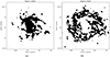 |
Fig. A.1. Spatial distribution of the highly star-forming R1 regime with ΣSFR > 3.8 M⊙ Gyr−1 pc−2(a) and the R2 regime dominated by diffuse and weakly star-forming ISM of IC 342 with ΣSFR < 3.8 M⊙ Gyr−1 pc−2(b). |
Pixel-by-pixel radio-FIR correlations for IC342.
All Tables
All Figures
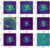 |
Fig. 1. IC 342 images from radio to FUV used in this work (see Table 2). |
| In the text | |
|
Fig. 2. LOFAR radio continuum map of IC 342 observed at 0.144 MHz overlaid with contours of the VLA 1.4 GHz emission. Contour levels are 3, 6, 12, 24, 32, 10−4 Jy/beam. Dashed circles indicate the positions of the background radio sources that were subtracted for this study. The beam size of 10.5″ is indicated in the bottom-left corner of the image. |
| In the text | |
|
Fig. 3. Maps of the thermal (left) and nonthermal synchrotron (right) radio continuum emission from IC 342 at the 4.8 GHz (top row), 1.4 GHz (middle row), and 0.144 GHz (bottom row) frequencies, all at a 25″ angular resolution. Color bars show the intensities in units of Jansky per pixel. |
| In the text | |
|
Fig. 4. Synchrotron spectral index maps of IC 342 for α[1.4 − 4.8] (top), α[0.14 − 4.8] (middle), and α[0.14 − 1.4] (bottom) overlaid with contours of the 22 μm emission indicating star-forming regions. Contour levels are 2, 4, 6, 8, and 10 × 10−4 Jy/pix. |
| In the text | |
|
Fig. 5. Histogram of the synchrotron spectral index in the high-frequency interval of 1.4 ≤ ν ≤ 4.8 GHz (blue), the entire frequency interval of 0.14 ≤ ν ≤ 4.8 GHz (red), and low-frequency interval of 0.14 ≤ ν ≤ 1.4 GHz (black). |
| In the text | |
|
Fig. 6. Magnetic field strength maps in IC 342. Strength of the total magnetic field Btot obtained using the synchrotron emission at 1.4 GHz in IC 342 at a 25″ angular resolution (top). Also shown are maps of the ordered Bord (middle) and turbulent Btur (bottom) magnetic field strengths. The bars on the right of each image show the magnetic field strength in μG. Contours show the 22 μm emission at levels of 2, 4, 6, 8, and 10 × 10−4 Jy/pix. |
| In the text | |
|
Fig. 7. Logarithmic ratio of the 70 μm emission to the radio synchrotron intensity at 1.4 GHz (q1.4, top) and 0.14 GHz (q0.14, bottom) at a 25″ angular resolution. Contours show the 22 μm emission at levels of 2, 4, 6, 8, and 10 × 10−4 Jy/pix. |
| In the text | |
|
Fig. 8. Histogram of q1.4 (red) and q0.14 (blue) in star-forming regime of the ISM (R1) in IC 342. The median value of each distribution (solid lines) and their 1-sigma intervals (solid lines) are also indicated. |
| In the text | |
|
Fig. 9. Multi-scale correlation between the radio continuum emission and the FIR bands at 70 μm (top), 100 μm (middle), and 160 μm (bottom). In each panel, the solid horizontal line shows rw = 0.5, and vertical lines indicate its corresponding scales of occurrence (lbreak) for different radio and FIR pairs. |
| In the text | |
|
Fig. 10. Logarithmic ratio of the 70 μm to the radio synchrotron emission at 1.4 GHz (q1.4, circles) and 0.14 GHz (q0.14, triangles) versus star formation surface density ΣSFR (M⊙ yr−1 kpc−2) in regime R1. Solid lines show bisector OLS fits. The color bar shows the spectral index between 0.14 and 1.4 GHz α[0.1 − 1.4]. |
| In the text | |
|
Fig. 11. FIR emission at 70 μm (top) and synchrotron emission at 1.4 GHz (bottom) versus SFR surface density ΣSFR (M⊙ yr−1 kpc−2) in the star-forming regime (R1). Solid lines show bisector OLS fits. |
| In the text | |
|
Fig. 12. Total, turbulent, and ordered magnetic field strength obtained using the synchrotron emission at 1.4 GHz (circles) and 0.14 GHz (triangles) versus SFR surface density ΣSFR (M⊙ yr−1 kpc−2). Solid lines show bisector OLS fits. For better visualization, the turbulent magnetic field strength has been shifted by 0.2 along the y-axis. |
| In the text | |
|
Fig. 13. Synchrotron spectral index and its relationship with star formation and magnetic field strength. Top: Synchrotron spectral index obtained at different frequency intervals (α[0.1 − 1.4], α[1.4 − 4.8] and α[0.1 − 4.8]) versus star formation surface density ΣSFR (M⊙ yr−1 kpc−2). Lines show bisector OLS fits. Middle: Same spectral indices versus the total magnetic field strength. Bottom: Synchrotron spectral index α[1.4 − 4.8] versus magnetic field after compensating both for the effect of the SFR. |
| In the text | |
|
Fig. 14. Diffusion length of the CREs ldif obtained from observations versus what is expected from the theoretical diffusion model for the case of tCRE = tsyn (a, Eq. (13)) and tCRE = tesc (b, Eq. (14)). Also shown is the correlation of ldif with the ordered magnetic field (c). |
| In the text | |
|
Fig. A.1. Spatial distribution of the highly star-forming R1 regime with ΣSFR > 3.8 M⊙ Gyr−1 pc−2(a) and the R2 regime dominated by diffuse and weakly star-forming ISM of IC 342 with ΣSFR < 3.8 M⊙ Gyr−1 pc−2(b). |
| In the text | |
Current usage metrics show cumulative count of Article Views (full-text article views including HTML views, PDF and ePub downloads, according to the available data) and Abstracts Views on Vision4Press platform.
Data correspond to usage on the plateform after 2015. The current usage metrics is available 48-96 hours after online publication and is updated daily on week days.
Initial download of the metrics may take a while.