| Issue |
A&A
Volume 639, July 2020
|
|
|---|---|---|
| Article Number | A51 | |
| Number of page(s) | 26 | |
| Section | Extragalactic astronomy | |
| DOI | https://doi.org/10.1051/0004-6361/201937246 | |
| Published online | 06 July 2020 | |
The XMM deep survey in the CDFS
XI. X-ray spectral properties of 185 bright sources⋆
1
Institut de Ciències del Cosmos (ICCUB), Universitat de Barcelona (IEEC-UB), Martí i Franquès, 1, 08028 Barcelona, Spain
e-mail: kazushi.iwasawa@icc.ub.edu
2
ICREA, Pg. Lluís Companys 23, 08010 Barcelona, Spain
3
INAF-Osservatorio di Astrofisica e Scienza dello Spazio di Bologna, via Gobetti 93/3, 40129 Bologna, Italy
4
Dipartimento di Fisica e Astronomia, Università di Bologna, Via Gobetti 93/2, 40129 Bologna, Italy
5
Department of Astonomy and Astrophysics, 525 Davey Lab, The Pennsylvania State University, University Park, PA 16802, USA
6
Institute of Gravitation and the Cosmos, The Pennsylvania State University, University Park, PA 16802, USA
7
Department of Physics, 104 Davey Laboratory, The Pennsylvania State University, University Park, PA 16802, USA
8
INAF-Osservatorio Astrofisico di Arcetri, Largo E. Fermi, 5, 50125 Firenze, Italy
9
Instituto de Física de Cantabria (CSIC-UC), Avenida de los Castros, 39005 Santander, Spain
10
Combient MiX AB, PO Box 2150, 40313 Gothenburg, Sweden
11
European Southern Observatory, Karl-Schwarzschild-Str. 2, 85748 Garching bei München, Germany
12
National Observatory of Athens, V. Paulou & I, Metaxa 15236, Greece
13
Agenzia Spaziale Italiana-Unità di Ricerca Scientifica, via del Politecnico, 00133 Roma, Italy
14
Dipartimento di Fisica, Università degli studi di Napoli Federico II, via Cinthia, 80126 Napoli, Italy
15
INAF – Osservatorio Astronomico di Capodimonte, Via Moiariello 16, 80131 Napoli, Italy
16
INFN – Sezione di Napoli, Via Cinthia 9, 80126 Napoli, Italy
Received:
3
December
2019
Accepted:
10
April
2020
We present the X-ray spectra of 185 bright sources detected in the XMM-Newton deep survey of the Chandra Deep Field South with the three EPIC cameras combined. The 2–10 keV flux limit of the sample is 2 × 10⁻¹⁵ erg s−1 cm−2. The sources are distributed over a redshift range of z = 0.1−3.8, with 11 new X-ray redshift measurements included. A spectral analysis was performed using a simple model to obtain absorbing column densities, rest-frame 2–10 keV luminosities, and Fe K line properties of 180 sources at z > 0.4. Obscured AGN are found to be more abundant toward higher redshifts. Using the XMM-Newton data alone, seven Compton-thick AGN candidates were identified, which set the Compton-thick AGN fraction at ≃4%. An exploratory spectral inspection method with two rest-frame X-ray colours and an Fe line strength indicator was introduced and tested against the results from spectral fitting. This method works reasonably well to characterise a spectral shape and can be useful for a pre-selection of Compton-thick AGN candidates. We found six objects exhibiting broad Fe K lines out of 21 unobscured AGN of best data quality, implying a detection rate of ∼30%. Five redshift spikes, each with more than six sources, are identified in the redshift distribution of the X-ray sources. Contrary to the overall trend, the sources at the two higher redshift spikes, at z = 1.61 and z = 2.57, exhibit a puzzlingly low obscuration.
Key words: atlases / galaxies: active / X-rays: galaxies
Full Table 1 and data for Fig. 2 are only available at the CDS via anonymous ftp to cdsarc.u-strasbg.fr (130.79.128.5) or via http://cdsarc.u-strasbg.fr/viz-bin/cat/J/A+A/639/A51
© ESO 2020
1. Introduction
To understand the evolution of galaxies and black hole growth in the Universe, sensitive observations of distant galaxies are essential, particularly of those that are heavily obscured, and deep X-ray observations play an important role for studying the population of active galactic nuclei (AGN) with obscuration (Brandt & Hasinger 2005; Brandt & Alexander 2015). The Chandra Deep Field South (hereafter CDFS, Giacconi et al. 2001) is one of the key fields that are subject to multiwavelength deep surveys. X-ray observations with the Chandra X-ray Observatory (Chandra) now reach a 7 Ms exposure, which makes it the deepest X-ray survey field (Luo et al. 2017). XMM-Newton observed the CDFS in the period of 2008–2010, in addition to the early observations in 2001–2002, and the survey overview is presented in Comastri et al. (2011). The resulting total exposure time is about 2.5 Ms. The 2–10 keV bright source catalogue of 339 sources, in which the flux limit is ∼1 × 10⁻¹⁵ erg s−1 cm−2, was published by Ranalli et al. (2013). Various works on specific subjects or individual sources from the survey data have been carried out (Iwasawa et al. 2012a; Georgantopoulos et al. 2013; Falocco et al. 2013, 2017; Castelló-Mor et al. 2013; Antonucci et al. 2015; Iwasawa et al. 2015; Vignali et al. 2015). In this paper, we present X-ray spectra of the brightest 185 sources, obtained from the EPIC cameras of XMM-Newton (Strüder et al. 2001; Turner et al. 2001), along with their basic spectral properties. While the 7-Ms Chandra exposure of the CDFS reaches a fainter flux limit and provides good quality spectra of individual sources (Luo et al. 2017; Liu et al. 2017), this XMM dataset provides an independent resource for investigating the X-ray source properties.
Between the XMM-Newton and Chandra datasets, comparable source counts were acquired for a source located in the central part of the survey field at intermediate energies, that is, ∼2 keV, given the respective effective areas and exposure times. However, the background sets their overall data quality apart. The sharp point spread function (PSF) of Chandra data not only helps push the detection limit of a point-like source to the faint flux level, but it also improves the overall spectral data quality over that of XMM-Newton since the data extraction aperture in the former is much smaller and, thus, the background is proportionally low, even if the respective detector background levels (per area) are comparable. Moreover, it is unfortunate for the XMM-Newton observations that the quiescent level of the background of the EPIC cameras during the 2008–2010 period was elevated to approximately twice that of the earlier observations, likely due to variations in Solar activity (Ranalli et al. 2013).
However, the XMM-Newton data can still prove competitive when it comes to measurements of Fe K lines, an important probe for AGN surrounding. The EPIC cameras of XMM-Newton have spectral resolution that are better than the ACIS-I detector used in the Chandra observations by a factor of 1.5–2. Apart from a few Compton-thick AGN, Fe K lines in most of AGN spectra lie above strong continuum emission. The higher spectral resolution gives a better sensitivity to a narrow emission line in these sources. Liu et al. (2017) detected Fe K lines in 50 sources from the Chandra 7-Ms dataset. We detected Fe lines in a comparable number of sources, namely, 71. Fe K emission is the most prominent spectral line in the X-ray band but the study of its properties in AGN has been limited mostly to objects in the local Universe (e.g. Bianchi et al. 2009) because, for example, of insufficient photon counts of distant, faint sources. The deep XMM-CDFS data allow us to extend it beyond the redshift of z = 1.
This paper presents the X-ray spectral atlas of the XMM-CDFS sources with which we try to facilitate a quick, visual inspection of overall spectral shape and the iron line feature of individual sources, using combined data from the three EPIC cameras. We examine the possible evolution of AGN obscuration and Fe line properties and search for Compton-thick AGN candidates, based on basic but homogeneous spectral fitting. We also test an exploratory spectral inspection method using two rest-frame X-ray colours and an Fe K line strength indicator for selecting Compton-thick AGN candidates.
The paper is organised as follows. A brief description of 185 X-ray sources is presented in Sect. 2, followed by the spectral atlas of these sources in Sect. 3. The X-ray properties obtained from spectral fitting are reported in Sect. 4, followed by the description of the exploratory analysis method and its results in Sect. 5. Composite spectra of various subsamples are shown in Sect. 6. Finally, in Sect. 7, a discussion of Compton-thick AGN, the evolution of AGN obscuration, X-ray sources in redshift spikes, and Fe K lines is provided. In the Appendix sections, supplemental details on X-ray redshift measurements, the exploratory analysis, spectral stacking methods, and the spectral atlas figures are given.
The cosmology adopted here is H0 = 70 km s−1 Mpc−1, ΩΛ = 0.72, ΩM = 0.28 (Komatsu et al. 2011).
2. XMM-CDFS sources
We present X-ray spectra of the brightest 185 sources in the 2–10 keV band from the XMM-CDFS survey, obtained from the EPIC cameras. The sources were selected using a combined criteria of 8σ detection and the observed 2–10 keV flux, f2−10 > 1.8 × 10⁻¹⁵ erg s−1 cm−2, from the 339 sources in the 2–10 keV XMM-CDFS source catalogue of Ranalli et al. (2013). The source identification number listed in the catalogue paper by Ranalli et al. (2013) are used with the prefix “PID”. There is redshift information provided, either spectroscopic or photometric, for all the sources.
The majority of the redshift information was taken from the CDFS Chandra 7 Ms source catalogue by Luo et al. (2017). When a secure spectroscopic redshift was not available, we inspected the X-ray spectra for a characteristic line or absorption feature in the Fe K band to try to obtain an X-ray spectroscopic redshift. X-ray redshift estimates have already been obtained for six sources with z ≥ 1.6 in Iwasawa et al. (2012a) and Vignali et al. (2015). We have a further 11 sources for which X-ray spectroscopic redshifts are adopted. The procedure of obtaining an X-ray redshift is described in Sect. 4.3 and a brief summary of the new 11 sources with X-ray redshifts is given in Appendix A. Consequently, among the total 185 sources, we have 135 sources with optical spectroscopic redshifts, 33 sources with photometric redshifts and 17 sources with X-ray spectroscopic redshifts. The redshift ranges from z = 0.11 to z = 3.74. Their distribution is shown in Fig. 1. A few redshift spikes, which may not be clear in the histogram, are identified and X-ray sources in the spikes are discussed in Sect. 7.3.
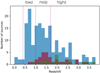 |
Fig. 1. Redshift distribution of the 185 XMM-CDFS sources (blue). The majority are spectroscopic redshifts. Photometric redshifts and X-ray redshifts are overdrawn in red and green, respectively. The redshift ranges of lowz, midz and highz are labeled and their boundaries are marked by dashed lines. |
The source identification number, adopted redshift, redshift type (spectroscopic, photometric or X-ray), along with the source characteristics obtained in the spectral analysis, are presented for the 185 sources in Table 1, which is shown here for only the first five sources. The full table is available in electronic form at the CDS and has a few extra columns for Fe K line detection flag, the spectral data quality indicator, the Chandra source identification numbers of Luo et al. (2017) and Xue et al. (2016), along with the classification of radio-loud AGN. We note that the XMM detected emission of PID 301 is composed of two X-ray sources resolved by Chandra. The redshift quoted in the table is the photometric redshift for the absorbed, hard source. The softer part of the spectrum is dominated by the other source with spectroscopic redshift z = 0.566.
185 XMM-CDFS sources.
3. EPIC spectral atlas
We constructed low-resolution spectra of all the 185 sources in the 0.5–7 keV band, as observed in a uniform manner for a visual inspection of broad-band spectral shape. Figure 2 shows first three spectra in PID number and the remaining 182 spectra can be found in Appendix D. All the spectra are plotted in 24 identical, logarithmically equally spaced energy intervals. The data are plotted in the flux density units, 10−15 erg cm−2 s−1 keV−1, and the range of flux density is always kept to 2 orders of magnitude to facilitate a visual comparison between sources. Three dotted, vertical lines drawn in each panel indicate a rest-frame of 3 keV, 6.4 keV and 1 keV, as expected from the adopted redshift. These energy lines are intended to guide the three key rest-frame energies in the observed spectra of sources at various redshifts. Each spectral panel shows PID, adopted redshift, and its category (sp: spectroscopic; ph: photometric; or x: X-ray) in parenthesis.
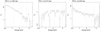 |
Fig. 2. Observed 0.5–7 keV spectra of 185 XMM-CDFS sources, shown in order of PID number. Only the first three spectra are shown here and the remaining 182 spectra can be found in Appendix D. Flux density is in units of 10−15 erg s−1 cm−2 keV−1. The energy scale is as observed and the three, vertical dotted lines indicate the rest-frame energies of 3 keV, 6.4 keV and 10 keV, expected from the adopted redshift. |
Since XMM-Newton carries three EPIC cameras, namely, pn, MOS1, and MOS2, each with different energy responses, we corrected a count-rate spectrum from each camera for the detector response (the effective area and the energy redistribution) and the Galactic absorption (NH = 9 × 1019 cm−2, Dickey & Lockman 1990) with the same method used in Iwasawa et al. (2012b) before averaging them using the observed-frame 1–5 keV source net counts as a weight. Then these averaged spectra were converted to flux-density units. Among the 185 sources, 169 have data from all the three cameras while the rest have of two cameras of the three. All the spectral data in ASCII format are available from the CDS.
4. Spectral fittings of individual sources
4.1. Absorption and X-ray luminosity
Spectral data were prepared for broad-band spectral fitting to extract basic continuum spectral parameters, namely, intrinsic cold absorption column density, NH, spectral slope for some sources, and Fe K line strength. We set 2–20 keV as the rest-frame energy range where each spectrum is investigated and we defined 27 logarithmically equally-spaced intervals to cover the energy range (note: they are different from the 24 intervals in the observed 0.5–7 keV band used for the spectral atlas). Due to the limited XMM-Newton bandpass, the rest-frame energies that the EPIC cameras cover differ depending on the source redshift: data for lower redshift sources do not reach rest-frame 20 keV, conversely, data below the rest-frame 2 keV for highest redshift sources are not covered. We divided all the sources, excluding 5 sources with z ≤ 0.4, into three redshift groups, lowz (0.4 < z ≤ 1.0); midz (1.0 < z ≤ 1.7); and highz (1.7 < z ≤ 3.8), and adopted reduced energy ranges for the lowz (2–10 keV) and midz (2–14 keV) groups and the full 2–20 keV range to the highz group. Then we rebinned individual spectra with energy intervals corresponsing to the fixed rest-frame energy intervals defined above (Table 2). The lower bound of the rest energy of 2 keV is covered by the EPIC cameras for all the sources, including the highest redshift object, and gives the data a sensitivity to the absorbing column density of NH = 1 × 1022 cm−2, which is conventionally used to divide obscured and unobscured X-ray sources. The “soft excess” emission is often present in unobscured AGN and this component emerges below 2 keV. The 2 keV-limit eliminates the soft excess emission affecting a continuum measurement. This bandpass limit, however, makes the spectra insensitive to absorption by a column density smaller than NH ≃ 1 × 1021 cm−2.
Three redshift groups.
The spectral model we use is a simple absorbed power law. The Galactic absorption and a narrow Gaussian at the fixed rest-frame energy of 6.4 keV for an iron line are also included. For most sources, the power-law slope1 is assumed to be α = 0.8 (e.g. Nandra & Pounds 1994; Ueda et al. 2014) and the column density, NH, in the line of sight is fitted (Table 1). There are a few sources that have a clearly steeper continuum slope. These sources were pre-selected by the rest-frame (2–5 keV)/(5–9 keV) colour (=S/M, see the following Sect. 5.1). As α = 0.8 corresponds to S/M = 2.94, when a source has S/M > 2.9, it was considered to be a steep-spectrum source candidate and both α and NH were fitted (Sect. 4.2).
All the spectral fitting was performed using count rate spectra with background correction from the three EPIC cameras (or two cameras when data from not all three cameras are available) jointly using the model folded through the respective detector responses. A variable constant factor is applied to each camera, primarily to accomodate the inter-camera calibration errors, but sometimes also to take into account larger variations between the cameras, which are dominated by aperture differences caused by the detector gap, etc. The rest-frame 2–10 keV luminosity as observed (L2−10) and that corrected for absorption ( ) are estimated from this absorbed power-law (Table 1). The median value of the luminosities from the three cameras (because of the varying normalising constants) was taken. The best-fitting model for each source was recorded and used later as the continuum model to investigate the Fe K line further with the higher resolution, narrow band data (Sect. 4.4.1).
For sources in which a large absorbing column (NH > 5 × 1023 cm−2) is found, their NH values and absorption-corrected luminosities are re-evaluated, assuming a toroidal geometry for an absorber, since the effects of Compton scattering become non-negligible and alter the shape of their observed spectra. We use the etorus model (Ikeda et al. 2009) in which the effects of Compton scattering are included by Monte Carlo simulations assuming a torus type of absorber. Since we do not know the geometry of the absorbing torus (neither do the data have sufficient constraining power), we assume an edge-on torus with a half opening angle of 30°. In this particular torus geometry, the primary spectral alteration is due to an addition of reflected light from the inner wall of the torus which penetrates through the near side of the torus (and therefore gets absorbed) before reaching an observer (e.g. Reflection 1 in Ikeda et al. 2009, Fig. 2). The main effect is a deepened Fe K absorption edge at a given NH, resulting in the new NH values being slightly smaller than the original values. These refitted values of NH and absorption-corrected luminosities are reported in Table 1. We note that depending on the assumption of the torus geometry, NH values can also shift to higher values. In the case of a grazing view of the torus edge of an inclined torus with a wide opening angle, for example, 60° (but with the central source still hidden), its inner wall is well-exposed to an observer. Directly visible reflected light from the inner wall (e.g. Reflection 2 in Ikeda et al. 2009) fills in the softer energies below the Fe K band of the spectrum in this NH range where the primary continuum is suppressed by absorption. This causes the line-of-sight absorption model to underestimate the real value of NH, that is, a larger NH, would be obtained when replacing with this inclined torus. For example, log  [cm−2] given for PID 144 (Norman et al. 2002; Comastri et al. 2011) could go up to log
  by changing the torus configuration. Similar amounts of shift in log NH are seen in other five sources with log NH > 23.8 (PID 66, 131, 245, 252, 316). In the latter torus configuration, the 68% error region of NH for all the six sources contains log NH = 24. Thus, with no knowledge of the torus geometry, ∼0.1 dex of uncertainty in NH always exists in this NH regime. Furthermore, the spectra are likely more complex, due to scattered light and partial covering etc., than the simple model we apply at high NH.
The NH distribution is plotted in Fig. 3. Median values of log NH, in units of cm−2, are 22.48 for all the sources, 21.98 for the lowz, 22.38 for midz, and 22.84 for highz groups (see Table 3), suggesting an increasing trend of absorption toward higher redshifts, as illustrated by the box-and-whisker plot in Fig. 3. This trend is translated to (on average) larger absorption corrections of luminosity for sources at higher redshift, as shown in Fig. 4. The median values of observed luminosity, absorption-corrected luminosity for each redshift group are given in Table 3. As for the obscured AGN fraction, when sources with NH > 1 × 1022 cm−2 (the 1σ lower limits need to be larger than 1 × 1022 cm−2) are counted as obscured AGN,  ,
,  , and
, and  for lowz, midz and highz sources, respectively2.
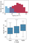 |
Fig. 3. Upper panel: distribution of best-fit NH values obtained for all the 180 sources at z > 0.4. The histogram in red shows the NH distribution of absorption detected sources, while the blue histogram shows that of the upper limits. We note the limited but uniform sensitivity of our spectra to NH due to the rest-frame bandpass (see text). Lower panel: box-and-whisker plots of NH measurements for the lowz, midz and highz groups. Following the normal convention, the box represents the inter quatile range (the middle 50%), the bar in the middle represents the median value, and the whiskers show the range of the minimum and the maximum of the distribution. |
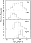 |
Fig. 4. Rest-frame 2–10 keV luminosity distributions for all the 180 sources, the lowz, midz and highz sources. The solid line histograms denote the distribution of absorption-corrected luminosity, while the dotted lines are for luminosity as observed. |
Median properties of sources in the three redshift ranges and three redshift estimate types.
The median properties for sources with spectroscopic, photometric and X-ray redshift estimates are also shown in Table 3. A comparison between sources with spectroscopic and photometric redshifts is discussed later (Sect. 6.2). X-ray redshifts are derived from an Fe K absorption edge in many cases, which naturally result in the large median absorbing column.
4.2. Steep spectrum sources
As mentioned above, sources that have a possibly steep continuum slope, i.e., α > 0.8, were selected by S/M > 2.94 and the absorbed power-law fit was performed by allowing both the slope and absorption to vary. Five sources (PID 40, 86, 243, 290, 375 and 407) with noisy data which do not have constraining power for both slope and NH were excluded here. Measured slope (energy index α) for these 22 steep-spectrum source candidates are reported in Table 4.
Steep spectrum sources.
4.3. Spectral slopes of radio-loud AGN
Some fraction of our sources are expected to be radio-loud AGN. Their X-ray spectrum may have a contribution of jet, resulting in a harder spectrum than the standard slope of α = 0.8 assumed for the above spectral analysis. Among the 185 sources, 16 sources are found to match radio sources classified as radio-loud AGN in Bonzini et al. (2013). This makes the fraction of radio-loud AGN to be ∼9%. The radio source identification number (RID) of Bonzini et al. (2013) for the 16 sources are listed in the online version of Table 1. We note that the radio-loud AGN classification by Bonzini et al. (2013) follows Padovani et al. (2011) and is based on excess radio emission above the radio (1.4 GHz) – mid-infrared (24 μm) luminosity correlation for star-forming galaxies, instead of the classical radio-loudness parameter R (Kellermann et al. 1989) defined by the radio to optical ratio, which could pose a problem for obscured AGN (we refer to e.g. Lambrides et al. 2020 for effects of obscuration on the AGN classification schemes using multiwavelength comparisons). These 16 radio-loud AGN include the two brightest X-ray sources in the field, PID 203 and PID 319, and the optically faint, X-ray bright obscured quasar at z = 1.6, PID 352 (Vignali et al. 2015). PID 319 and PID 352 are reported to have an extended radio morphology (Hales et al. 2014; Huynh et al. 2015): PID 352 is a powerful radio galaxy with log P1.4 = 27.1 [W Hz−1] with a double radio-lobe (Vignali et al. 2015).
Out of the 16 radio-loud AGN, ten sources have X-ray absorption of NH ≥ 1022 cm−2, which makes it diffiult to determine their intrinsic X-ray slopes. We reexamined the remaining six unobscured sources for their spectral slopes. Three sources, PID 182, PID 190, and PID 359 are found to have slightly hard slopes, α = 0.55–0.67 (Table 5), and therefore a jet contribution to the X-ray emission is suspected. These three have the 1.4 GHz radio power of log P1.4 = 24.6–26.0 [W Hz−1] for our adopted redshits. The other three, PID 203, PID 319 and PID 407 have X-ray slopes α = 0.8–0.9, similar to the standard radio-quiet AGN slope. The former two are the bright X-ray sources and exhibit broad Fe K emission (Iwasawa et al. 2015), suggesting that the disc emission dominates their X-ray spectra. The spectral slope of PID 407 is not well constrained but the source is one of the possible steep-spectrum sources selected in Sect. 4.2.
Unobscured radio-loud AGN with a hard spectrum.
4.4. Fe K lines
4.4.1. Narrow Fe K emission
The spectral binning used for the broad band spectral fits includes a rest-frame 6.1–6.6 keV interval where a neutral Fe K line at 6.4 keV would fall. In general, when a adopted source redshift is correct, the 6.4 keV line intensity derived from the broad-band fit is expected to be correct even with this low-resolution setting. However, when, for example, an adopted photometric redshift is slightly wrong, or the Fe K emission comes from highly ionised iron, Fe XXV or Fe XXVI, some line photons fall out of the Fe K interval, leading to an inaccurate line measurement. To assure more reliable line measurements, we optimise the resolution of the spectrum in a limited energy range. The source spectra were rebinned with 30 eV intervals in the observed frame and data corresponding to the rest-frame 5–8 keV were used. This choice of spectral resolution gives sufficient oversampling for a narrow Fe line from high-redshift sources at z ∼ 3 (for which a Fe line would appear at an energy range where the spectral resolution is ∼100 eV in FWHM) as well as lower redshift sources. A high-ionisation Fe K line can be distinguished from a 6.4 keV cold line. In case of sources with loosely constrained photometric redshifts, fitting a line energy could give a more precise redshift. When this happened, the broad-band fitting was repeated to revise the absorbing column density and luminosity, using the updated X-ray redshift information.
The best-fitting absorbed power-law obtained for each source in the previous subsection was used as the continuum model. A narrow Gaussian was fitted with one of the line energies of 6.4 keV, 6.7 keV and 6.97 keV appropriate for cold Fe, Fe XXV, and Fe XXVI, respectively, whichever describes the observed line best, with the normalisation set as a free parameter. The adopted line centroid and rest-frame equivalent width (EW) are reported in Table 1. For Fe line driven X-ray redshift measurements, for example, for PID 352 (Vignali et al. 2015) and PID 215, the Fe K line is assumed to be a cold line at 6.4 keV, since most Fe lines in our sample are found at that energy, as shown below, and the source redshift was fitted using these fine resolution spectra.
There are 71 sources with Fe K line detection at the 90% confidence level or higher. The majority (85%) of the lines are found at 6.4 keV and the rest are found at 6.7 keV and 6.97 keV with a comparable share. The distribution of Fe K EW stretches up to 3 keV but most lines have EW smaller than 0.6 keV (Fig. 5). The number of Fe K line sources increases to 119 when the detection threshold is relaxed to the 68% confidence level. The composition of line energy slightly changes and the fraction of the high-energy lines increases to 25%. The EW distribution of these sources is shown in the inset of Fig. 5 along with the upper limits for non-detected sources. It suggests that the majority of sources with no line detection have EW smaller than 0.2 keV and they would be populated increasingly toward smaller EW if the spectral sensitivity were sufficient.
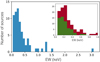 |
Fig. 5. Main: Fe K line equivalent width distributions of the 71 sources with the line detection at the 90% significance. Inset: the same distribution for the lines of the 68% line detection (red) and that for the upper limits of no detection (green). |
The median line EW for all the 180 sources inspected is 0.15 keV and the 68% interval of the bootstrap error is (0.14–0.17) keV (Table 3). No significant differences are found between the median EW values for the three redshift ranges.
4.4.2. Broad Fe K lines
We investigated how common broad Fe K features are among the unobscured AGN. Detecting a broad emission component requires high quality data because of the low contrast against the continuum (e.g. de La Calle Pérez et al. 2010). The two brightest sources (PID 203 and PID 319) in the field are unobscured AGN and indeed are broad Fe K line emitters (Iwasawa et al. 2015). As a guide for data quality, we adopt the signal to noise ratio of the rest-frame 3–10 keV (sne310: all the three EPIC cameras combined together3) and selected 21 unobscured sources with sne310 > 30 (including the above two brightest sources). Their rest-frame 2–10 keV, low-resolution spectra used in Sect. 4.1 were examined by modelling with a power-law continuum with a Gaussian line. The line centroid is fixed at 6.4 keV and the line width is fitted as well as line intensity. Because of our rest-frame spectral resolution setting, fits are sensitive to line broadening of σ ≳ 0.3 keV. This degree of broadening is appropriate for relativistically broadened line (e.g. Fabian et al. 2000). It also minimises the detection bias against high redshift sources in which Fe emission appears in energies where spectral resolution is lower than in lower redshift sources.
We detected line broadening (when the lower bound of the 90% confidence interval of the line width is positive) in six sources (Fig. 6) listed in Table 6, in which line widths, line EW, and the source flux measured in the observed 1–5 keV band can be found. In the other 15 sources, Fe lines are either unresolved or not detected. The broad-line detection rate is thus 29% in this sample of 21 sources. de La Calle Pérez et al. (2010) obtained a detection rate of 36% for the 31-source flux-limited FERO sample of nearby bright Seyfert galaxies observed with XMM-Newton. The 95% credible interval of our broad-line detection rate when the FERO result is used as a prior is 22–46%. The composite spectra of the six broad-line sources and the rest are shown in Fig. 7 to illustrate their differences.
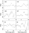 |
Fig. 6. Spectral data of six unobscured sources exhibiting broad Fe K features. The data are divided by the best-fit power-law. The source identification number is indicated. The upper four sources come from the lowz group while the lower two from the highz group (see Fig. 8). |
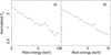 |
Fig. 7. Stacked spectra of the six broad Fe-line AGN (a) and the other 15 AGN (b) of the 21 unobscured sources with highest quality data. |
Six broad Fe K line sources.
Four of the six broad-line AGN belong to the lowz group (z < 1) while the remaining two lie at z = 1.8 and z = 2.6. There is no broad line detection in the nine sources in the intermediate redshifts between z = 0.9−1.8. The 21 sources we investigated are distributed over z = 0.5−2.6 (Fig. 8) with no bias towards low redshifts. Ten sources are clustered in the z = 1.6−2 range where one broad-line detection is recorded. The cumulative distribution functions of the sample and the broad-line detected sources in Fig. 8 seem largely deviated, suggesting a possible change in broad-line detection rate with redshift, or deficit of broad-line detection in the intermediate redshifts, although there is no obvious reason why it should change. A two-sample K − S test on the broad-line and non-broad-line samples give a p-value of 0.03, suggesting marginally that they might come from a different distribution.
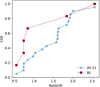 |
Fig. 8. Cumulative distribution functions of the redshifts of the 21 unobscured AGN with good data quality (blue circles) and those of the six in which broad Fe lines are detected (red squares). The redshifts of the sample AGN are spread over the range of 0.5–2.6 with some clustering in the z = 1.6–2 range. In contrast, broad line detections may be frequent at low redshifts (z < 0.9). |
Excluding the two brightest sources (PID 203 and PID 319) that feature exceptionally high-quality data, sne310 is comparable between the sources in the three redshift groups, indicating that data quality is unlikely to be the reason. If the data quality were all that mattered, the stacked spectrum of the 15 sources without individual broad-line detections would show a sign of line broadening, which is not seen (Fig. 7). Other properties such as median X-ray luminosities of the sources with and without broad-line detections are compatible (44.1 and 44.2 in log LX [erg s−1], respectively). Assuming external conditions are equal among the sample sources, the hypothesis that broad-line detection rate remains constant (∼29%) over the whole redshift range was examined by random sampling of six of the 21 redshifts. If we set four redshifts below z = 0.9 being found among the chosen six as a test measure given our observation, the p-value is estimated to be 0.01, indicating that our result is a relatively rare case under the hypothesis of the constant broad Fe K line detection rate. The complete lack of broad-line detection in the nine sources at z = 0.9–1.8 could occur at a probability of 0.03 by chance. Given the small sample size and the presence of two exceptionally bright sources with detected broad lines (PID 203 and 319, see Iwasawa et al. 2015), we withhold from drawing a conclusion on a possible redshift variation of broad Fe lines.
5. Exploratory spectral inspection with two X-ray colours and Fe K line strength indicator
We present a few quick-look spectral inspection methods and compare them with the results obtained from the conventional spectral fitting. When there are many spectra, a quick exploratory analysis using these methods may be useful for characterising the source population or to select sources with particular properties, such as Compton-thick AGN, if its accuracy turns out to be reasonable.
We used the same data that was prepared for the broad-band spectral fit. The data from the three cameras were averaged in the same way as those in the spectrum atlas (Sect. 3) and converted to flux density units and the energy scale was replaced by the rest-frame energy. The 27 energy intervals over the rest 2–20 keV range are denoted by indicies i = 0, 1…26. Hereafter we use these rest-frame flux density spectra for the analysis below.
5.1. Broad band continuum
First, we define three rest-frame energy bands: S: 2–5 keV; M: 5–9 keV; and H: 9–14 keV, where S, M, and H are integrated flux densities over the respective bands. Two X-ray colours, S/M and H/M, are then obtained. We note that there is no information on H for the sources in the lowz group because of the limited hard band data (see Table 2), and thus only S/M colours are available. The S/M colour is, in principle, a proxy for absorption if NH lies in the 1022 cm−2–1023 cm−2 range. Figure 9 shows a plot of S/M values against the best fitting NH. On both ends of the NH range, S/M values are saturated because the sensitivity of S/M to NH becomes weak due to the limited band passes of S and M, respectively. This results in a flatter correlation for the full range of log NH (21–24): the slope comes out as a = −1.10 ± 0.02 for S/M = a × log NH + b. The S/M ratio is sensitive in the middle part, that is, in the range of 22–23.3 in log NH, the slope becomes steeper (a ∼ −1.6) with a good fit (a χ2 test gives a chance probability of 2% with χ2 = 110.5 for 82 degrees of freedom). Thus, S/M can be considered as a reasonably good NH indicator in this range with the parameters, a = 1.60 ± 0.05 and b = 38 ± 1 in the above formula.
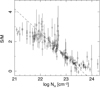 |
Fig. 9. S/M colours against best-fitting NH, obtained from the conventional spectral fit. The dashed line indicates the best-fitting relation in the range of 22–23.3 in log NH [cm−2] (see text). |
On the other hand, the H/M colour is sensitive to absorption only when NH exceeds 1023 cm−2, complementing S/M in the NH estimate at the higher value range. Figure 10 shows the colour–colour diagram of S/M and H/M for the midz and highz sources (similar to that in Iwasawa et al. 2012a). Predicted positions of sources with a power-law spectrum with α = 0.8 and various absorbing columns, as well as those with steeper continuum slopes (up to α = 1.2) and no absorption, are indicated in the figure. Sources located in the upper left corner are likely to be strongly absorbed sources, such as NH > 5 × 1023 cm−2.
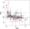 |
Fig. 10. Colour–colour (H/M – S/M) diagram for the midz and highz sources. The locus in dashed red line indicates the evolution of (S/M, H/M) when a power-law continuum of energy index α = 0.8 is modified by cold absorption with various column densities: log NH [cm−2] of 22, 22.5, 23, 23.5, 23.7, 23.85 and 24, as marked by cross symbols. Colours for a simple power-law with no absorption with α of 0.8, 1.0, and 1.2 are also marked. |
5.2. Estimate of Fe K band continuum and strong Fe line sources
Secondly, we consider a relatively crude method for noisy spectra to select sources with strong Fe K line emission. Strong Fe line emission with EW ≳ 1 keV is an unique characteristic of a reflection-dominated spectrum from heavily obscured AGN. This proposed method may help quickly select such strong Fe line sources.
With the adopted spectral binning, the i = 13 bin corresponds to the 6.0–6.6 keV range where a cold Fe K line (6.4 keV) would appear. The first step is to estimate the continuum level in the i = 13 bin using the data of neighbouring intervals. We adopt as the flux density in bin i = 10 at 4.9 keV (i = 16 at 8.2 keV) the median of the flux densities in bins i = 8–12 (i = 14–18). A logarithmic mean of these two values of flux density gives an estimate of the continuum level at the i = 13 bin. This operation is equivalent to obtaining a continuum level at i = 13 by applying a power-law running through the two median points because of the logarithmically equal intervals by design. A few examples of its application to real data can be found in Appendix B.
Thus we have the continuum level estimates in the Fe K band for all the sources. Taking the ratio of  , where f13 is the flux density of the source measured at i = 13 and
  is the estimated continuum level, gives a measure of excess emission in that interval, likely due to cold Fe K line emission. This ratio obtained for each source is given in Table 1. Since the i = 13 bin has an energy interval of 0.54 keV, R(Fe) and Fe K line EW would be related by R(Fe) = 1 + (EW/0.54), if the continuum estimate for the i = 13 bin is accurate. While the ratio being unity means no Fe line, selecting sources with R(Fe) > 2, for instance, results in their spectra having an Fe K line with EW > 0.54 keV.
We examine how R(Fe) is actually related to the EW measured by spectral fitting. First, the 71 sources with Fe lines of ≥90% detection (Sect. 4.4.1) were inspected (Fig. 11). The correlation between R(Fe) and EW is reasonably strong (r = 0.76). Fitting a linear relation of R(Fe) = α + βEW gives  and
and  . The fraction of outliers is about 5%. The intercept, α, is consistent with being 1. The slope, β, is slightly steeper than the expected value, β0 = 1/0.54 = 1.85 but is compatible. The uncertainty of the slope extending predominantly toward lower values indicates that the best-fit slope is largely driven by the single data point of large EW (∼3 keV of PID 215) which lies very close to the best-fit. Since the error interval was obtained by bootstrap, this implies that, when this data point is excluded, the relationship becomes flatter than the best-fit case and actually has a slope closer to the theoretical value. When the data range is limited to the crowded region on the bottom-left corner (right panel of Fig. 11), where 63/71 ≈ 90% of the sources are located, the correlation, albeit not very tight, still persists (r = 0.66). Re-fitting the linear model yields
  and
and  . There are not many catastrophic outliers among the sources with no or weak detection of Fe lines, as shown in Fig. 11. Therefore, statistically, R(Fe) performs as an approximate EW indicator as expected, with a dispersion of σ = 0.32 ± 0.02 among the detected lines.
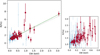 |
Fig. 11. Left: Fe K line strength indicator, R(Fe), against the Fe K line equivalent width (EW) obtained from spectral fitting. The filled squares (red) show data for Fe lines with the ≥90% detection while the circles (light blue) show data for weak/no detection for the whole sample. The dashed line indicates the fitted linear correlation (see text). The dotted line indicates the expected relation when the continuum level estimate of the i = 13 bin is accurate. Right: same plot for the crowded region of EW < 0.8 keV. |
Without spectral fitting, whether a given R(Fe) is associated with a significantly detected Fe line is not immediately clear. One measure is the error bars of R(Fe) itself, since it reflects the data quality of the Fe K line interval. Another is the broad-band data quality such as sne310 (for the rest-frame 3–10 keV). Although good quality data do not always guarantee a line detection, significant line detections tend to be more frequent as sne310 increases, for example, the probability of an Fe line being ≥90% significance is ≥74% when sne310 exceeds 30.
A few caveats on R(Fe) are: firstly, R(Fe) may sometimes overestimate EW when a source is heavily absorbed (a prime example is PID 316). A strongly absorbed spectrum exhibits a strong continuum curvature with a prominent continuum discontinuity around 7 keV due to an Fe K edge. Our simple interpolation method would then tend to place  lower than actually is, leading to an overestimate of R(Fe) (that is, the continuum discontinuity is viewed as part of an Fe line excess). A prime example is PID 316 but such a large deviation occurs only in two sources. Secondly, this method works only when the line photons fall well within the i = 13 bin (6.0–6.6 keV). Some sources show higher ionisation lines of Fe XXV and Fe XXVI (Sect. 4.4.1) which peak outside i = 13 and R(Fe) would fail to capture those lines. However, since the majority of the Fe K lines appear to be cold 6.4 keV lines, R(Fe) should work most of the time.
6. Composite spectra
We use spectral stacking to investigate average properties of the XMM-CDFS sources. Here we use normalised, individual rest-frame spectra to avoid a bias for bright sources. The normalising point is the i = 13 bin and each spectrum was normalised to the estimated continuum flux,  , obtained above for individual sources. Then we apply median stacking (see Appendix C). The 68% confidence interval for the median is estimated by bootstrap.
Figure 12 shows the composite spectrum of all the 180 sources. Fitting a simple absorbed power-law for the continuum gives  , NH =(1.3 ± 0.4)×1022 cm−2. We note that the fitted continuum precisely matches the value of unity at i = 13, suggesting the continuum level estimates of individual sources work well. A superposition of spectra with various degrees of absorption makes this hard spectrum. The presence of the absorption cut-off represented by the NH value above in the composite spectrum suggests that the NH distribution is not flat. Probably absorbed sources with NH greater than 1022 cm−2 dominate at the typical XMM-CDFS source flux. The Fe line peaks at i = 13 with wings on both sides. Fe line emission in the stacked spectrum is expected to be broadened to some degree since lines from sources at high redshifts are observed at low energies where the energy resolution, ΔE/E, of the EPIC cameras degrades (approximately ∝E−0.5) and they result in the artificial broadening (see e.g. Iwasawa et al. 2012b; Falocco et al. 2013). However, at z ∼ 2, the broadening is expected to be σ = 0.15 keV, a narrow line at 6.4 keV should be contained within the i = 13 interval. The presence of the wings hence means line broadening. The intrinsic line broadening is estimated to be σ = 0.27 ± 0.1 keV, when fitting a Gaussian and taking into account the effect of de-redshifting, assuming the median redshift of the sample z = 1.34. However, this is more likely due to the spread of the line energy than to many sources emitting intrinsically broad Fe lines, since we observed that Fe K line energies would be distributed around 6.4 keV with a dispersion of 0.26 keV when line energy is fitted instead of being fixed (Sect. 4.4.1). The line equivalent width is found to be
  keV, when the line broadenig is taken into account. When a narrow 6.4 keV line is assumed, the EW is reduced to 0.14 ± 0.04 keV.
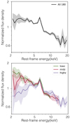 |
Fig. 12. Upper panel: rest-frame 2–20 keV composite spectrum of all the 180 sources at 0.4 < z < 3.8. The shaded area indicates 68% confidence intervals from bootstrap. Lower panel: same spectra for the lowz, midz and highz sources. |
6.1. Redshift evolution of spectra
We examine how the average spectral shape evolves between the three redshift groups (Table 2). The composite spectra for the lowz, midz and highz groups are shown in the lower panel of Fig. 12. It is readily clear that the spectrum becomes more absorbed as redshift increases. When an absorbed power-law, which has a common slope but variable NH between the three spectra, with a narrow Gaussian Fe line at 6.4 keV is fitted, the slope is found to be α = 0.52 ± 0.03, comparable to that obtained for the whole sample, as expected. NH values found in the three spectra are given in Table 7. The difference between NH for lowz and midz is marginal but that for highz is significantly larger. Although the harder spectral slope than that of unobscured AGN (α ∼ 0.8) means that the obtained NH values are not real values of typical absorbing columns, they show that absorption becomes progressively larger toward higher redshifts. This is in agreement with the NH distributions (Fig. 3) and the X-ray colour analysis (Fig. 13). The EW of Fe K lines are comparable between the three spectra: 0.14, 0.13 and 0.12 keV (±0.04 keV), respectively, as illustrated by Fig. 12.
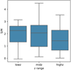 |
Fig. 13. S/M X-ray colour distributions of lowz, midz, and highz groups. |
Properties of composite spectra for sources in the three redshift ranges.
6.2. Spectroscopic vs. photometric redshifts
Figure 14 shows composite spectra of sources with spectroscopic and photometric redshift estimates, respectively. The median properties of these sources are given in Table 3. The number of sources with spectroscopic redshifts (131) is much larger than with photometric redshifts (32). We are aware that not all the photometric redshifts are reliable (the typical photometric redshift accuracy and outlier rate for the CDFS X-ray sources are σNMAD = 0.014 and η = 5.43%, respectively for the work by Hsu et al. 2014) but the presence of a clear Fe K line in the composite spectrum suggests that the majority of the photometric redshifts are of reasonable accuracy. An absorbed power-law fit gives results shown in Table 8. The sources with photometric redshift are faint in optical and the relatively hard composite spectrum agrees that their optical faintness is related to nuclear obscuration.
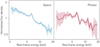 |
Fig. 14. Composite spectra of sources with spectroscopic redshifts and and photometric redshift estimates. |
Properties of composite spectra for sources with zsp and zph.
6.3. Unobscured AGN
X-ray obscured sources are defined as those with measured NH larger than 1 × 1022 cm−2, excluding those for which the lower bound of the 1σ interval of NH falling below the threshold. Unobscured sources are thus those with absorbing NH undetected or smaller than 1 × 1022 cm−2. There are 81 sources classified in this category. The median redshift and 2–10 keV luminosity of these sources are z̃ = 1.13 and log LX = 43.60 (log  ). The composite spectrum (Fig. 15) shows a power-law slope of α = 0.80 ± 0.02, NH = (4.2 ± 0.7)×1021 cm−2, and a Fe K line EW of 0.11 ± 0.01 keV.
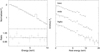 |
Fig. 15. Left panel: composite spectrum of all the 81 unobscured AGN with the best-fit power-law plus a narrow Gaussian for the Fe K emission and the residual in ratio of the data and the model. Right panel: composite spectra of unobscured sources in the lowz, midz and highz groups. The spectra are plotted with arbitrary offsets for clarity. |
Although the majority of these sources have spectroscopic redshifts (70 out of 81, most of the sources without spectroscopic redshifts are from the midz group), we construct a composite spectrum by using only sources with spectroscopic redshifts, in the interest of examining line broadening. The spectral shape agrees with that including the photometric redshift sources. No clear line broadening beyond the line bin (i = 13) is seen. Any redward excess emission above the continuum is < 2% in the 5–6 keV band and < 1% level in the 4–5 keV band, respectively. Falocco et al. (2017) performed a spectral stacking analysis of the same XMM-CDFS dataset. While their spectral stacking method is different from ours, the Fe line in their stacked spectrum for unobscured sources shows no broadening, in agreement with our result. The spectral analysis of the brightest individual sources shows the broad-line detection rate to be ∼30% (Sect. 4.3.2). The result of this composite spectrum suggests that no significant increase of the broad-line frequency occurs among the fainter sources.
Those 70 unobscured sources with spectroscopic redshifts are divided into the previously defined three redshift groups and their composite spectra are shown in the right panel of Fig. 15. The Fe line in the lowz spectrum is resolved and shows a blue wing. Fitting a Gaussian gives the line centroid of  keV and line width of σ = 0.35 ± 0.19 keV,
  keV. This is contrary to a red wing expected from a relativistically broadened line and probably due to distributed different line energies. The Fe lines in the spectra of midz and highz are in agreement with that of the total spectrum, confined within the i = 13 bin and are consistent with a narrow line at 6.4 keV with EW of 0.10 ± 0.03 keV and 0.12 ± 0.04 keV, respectively.
In order to see whether the anti-correlation between the EW of the narrow Fe K line and X-ray luminosity, or Iwasawa-Taniguchi effect (Iwasawa & Taniguchi 1993), seen in nearby unobscured AGNs (see also Page et al. 2004; Bianchi et al. 2007; Shu et al. 2012) holds, we constructed composite spectra in three luminosity ranges lowLx: 42.2–43.2; midLx: 43.2–44.0; and highLx: 44.0–45.2 in log LX [erg s−1]. The properties of the sample of three luminosity slices and results of spectral fits are given in Table 9. The narrow line component show comparable EW around 0.1 keV between the three luminosity ranges (Fig. 16). There is no trend of decreasing EW as increasing luminosity but also the EW are far above the relationship found for nearby AGN.
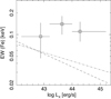 |
Fig. 16. Narrow Fe K line EW against X-ray luminosity obtained from the three luminosity slices of unobscured AGN (Table 9). The dashed and dash-dotted lines indicate the I-T effect obtained for nearby AGN by Bianchi et al. (2007) and Shu et al. (2012), respectively. |
Properties of composite spectra of unobscured AGN in three luminosity slices.
7. Discussion
7.1. Compton-thick AGN
Compton-thick AGN candidates were selected by two characteristic spectral features: (1) large absorbing column density NH ≥1024 cm−2; and (2) strong 6.4 keV Fe K line emission arising from reflection fom thick, cold matter.
On taking face values of NH measurements, the only source with NH exceeding 1024 cm−2 is PID 316. However, given the uncertainty in the NH measurements and the likely complexity of spectra at large NH discussed in Sect. 4.1, we select three more candidates (PID 66, PID 131, PID 245) with log NH ≥ 23.9 [cm−2], for which real values of their NH could reach the Compton-thick NH threshold.
On the other hand, sources with a reflection-dominated spectrum are often faint due to strong continuum suppression and their spectra are generally noisy. Consequently, blindly applying the strong Fe K line criterion could result in many false selection of Compton-thick AGN. In order to make the selection more reliable, we apply two complementary conditions in addition to the primary condition for strong Fe K line (EW ≥ 1 keV): (1) the line energy is consistent with 6.4 keV and at above 90% detection; and (2) hard X-ray colours: S/M < 1.5 and H/M > 0.5 (where available), to comply with the characteristics of a reflection-dominated spectrum in which Fe line emission arises from cold matter and the underlying continuum has a hard spectrum and extends well above 9 keV. This selection results in five sources (PID 102, PID 114, PID 131, PID 215, and PID 398). They are thus considered as reflection-dominated sources and their true NH would be in the Compton-thick regime. This alters the NH distribution in Fig. 3 slightly by stretching the larger NH end.
Among the above selected sources, we tentatively reserve the selection of PID 131, mainly because of the poor data quality: although the strong Fe K line seems to be real albeit lying close to the instrumental Al line at 1.5 keV of the MOS cameras (see Fig. D.1), the rest of the spectrum is very noisy. Combining the two selections (and discounting PID 131), the number of our Compton thick AGN candidates is seven out of 185 sources (∼4%). Previously suggested Compton-thick AGN candidates, PID 144 (Norman et al. 2002; Comastri et al. 2011), PID 147 (Comastri et al. 2011; Georgantopoulos et al. 2013), and PID 252 (Iwasawa et al. 2012a), for which Chandra data were also used, fall just below the NH threshold on the use of the XMM-Newton data alone and may add up the number of candidates to 10 (or 11 if PID 131 is included, ∼5–6%).
There are a few measurements of Compton-thick AGN fraction for nearby AGN using high-energy instruments, that is, Swift BAT and NuSTAR (Burlon et al. 2011; Ricci et al. 2015; Koss et al. 2016; Masini et al. 2018), as well as the independent measurements for CDFS sources (Tozzi et al. 2006; Brightman & Ueda 2012; Liu et al. 2017). They range from 3% to 22% and their distribution can be approximated by ∼Beta(3, 28)4. Using this as a prior, our seven detections yield the Compton-thick AGN fraction to be 4% with the 68%/95% credible intervals of (3.2–6.2)%/(2.4–7.8)% (Fig. 17). The XMM-CDFS value lies on the smaller side of the distribution of the previous measurements, largely coming from hard X-ray surveys of nearby AGN, but is similar to those derived from surveys with comparable depths: 5% at the flux limit of log f2−10 ≃ −15.0 [erg s−1 cm−2] (Tozzi et al. 2006); 5% at log f2−10 ≃ −15.1 (Brightman & Ueda 2012); 3% at log f2−10 ≃ −14.2 (Lanzuisi et al. 2018). We note that these values still have a selection bias against very Compton-thick sources. The AGN population synthesis models of the X-ray background give varying predictions of Compton-thick AGN fraction which depends on observed flux (e.g. Ueda et al. 2014; Akylas et al. 2012; Ballantyne et al. 2011; Gilli et al. 2007). In general, the Compton-thick AGN fraction starts to rise sharply below the flux limit at 10−14 erg s−1 cm−2. The typical 2-10 keV flux [erg s−1 cm−2] of our sources is log fX ∼ −14.4 and the flux limit is approximately −14.7. Our estimate of the Compton-thick AGN fraction is compatible with the models by Ueda et al. (2014) and Akylas et al. (2012) (but lower than those by Ballantyne et al. 2011; Ananna et al. 2019). The deeper Chandra 7-Ms dataset indeed gives a larger value of 8% (Liu et al. 2017).
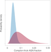 |
Fig. 17. Probability distributions for the Compton-thick AGN fraction obtained from the XMM-CDFS (in blue) using the beta distribution prior (in red) which approximates the distribution of previous measurements for nearby AGN using hard X-ray instruments and Chandra CDFS measurements (references are given in text). The best estimate is found at 0.04 with the 95% credible interval of (0.024–0.078). |
The above selection was made with the spectral fitting results on NH and Fe line EW (with the supplemental filtering by the X-ray colours). Then we investigate how those candidates can be selected only by the simplified analysis, that is, the two X-ray colours and R(Fe). Information on these values for each source is visualised in Fig. 18. The purpose is not to pin down Compton-thick sources but to sift out promising candidates for a further inspection by spectral fitting. By adjusting selection criteria for the above candidates, we propose the following criteria.
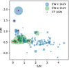 |
Fig. 18. Same X-ray colour-colour diagram as Fig. 10 with information of R(Fe) added by the symbol size (the larger the size, the larger the R(Fe) value), to illustrate the Compton-thick AGN selection by the X-ray colours and R(Fe) alone (without spectral fitting). The error bars of the X-ray colours are omitted for clarity. Sources with strong Fe K lines (EW ≥ 1 keV, measured by spectral fitting) are distinguished by colour. The seven Compton thick AGN candidates are marked by red triangles. Requiring S/M < 1.5 and H/M > 0.5 ensures a hard spectrum of a reflection-dominated source. |
(1) [S/M < 1.5 and H/M > 0.9]: to select sources with large NH.
This colour selection select 10 sources, PID 24, 30, 59, 66, 142, 147, 180, 245, 252 and 316. Their measured log NH ranges from 23.38 to 24.23 [cm−2]. All the four Compton-thick AGN selected by NH are included, along with other previously suggested candidates PID 147 (Comastri et al. 2011; Georgantopoulos et al. 2013), PID 252 (Iwasawa et al. 2012a).
We note the very hard X-ray colours on PID 59 (S/M = 0.88, H/M = 1.16). This source has a poorly constrained photometric redshift 2.881 (the 68% uncertainty range 1.04–4.81) and its spectrum shows a possible line-like feature of which energy does not match 6.4 keV for the adopted redshift. If this was identified with a Fe K line, this source would be another Compton-thick AGN candidate.
(2) [R(Fe) > 2.4 and S/M < 1.5 and H/M > 0.5]: to select reflection-dominated spectrum source with a strong Fe K line.
The selected sources are PID 66, 102, 114, 131, 144, 215, 221, 316, 324, and 398. Without spectral fitting, we would not know whether the Fe K line energy is 6.4 keV nor whether the line detection is significant, but all the six candidates selected by large EW (Fe K) are included. A strong continuum discontinuity due to an Fe K edge, when NH is large, could lead to a large R(Fe), as pointed out above. The rest of the sources exhibiting “not sufficiently strong” Fe lines were selected for this reason. The well-known Compton-thick AGN candidate PID 144 (Norman et al. 2002; Comastri et al. 2011) and other previously suggested candidates, PID 147 (Comastri et al. 2011; Georgantopoulos et al. 2013) and PID 324 (Georgantopoulos et al. 2013), are present in the selected sources.
By design the above two criteria select all the spectral fitting-based, Compton-thick AGN candidates (supposing they are “true positives” here). The number of sources selected by these criteria is 19, indicating that they do not pick up too many false positives (12). The false positives include Compton-thick AGNs (PID 144, 147, 252, and 324), previously suggested by a combined analysis of Chandra or XMM-Newton and Chandra. Therefore, the X-ray colour + R(Fe) selection may work as a pre-selection method. Figure 19 shows the composite spectrum of the seven Compton-thick AGN candidates, overplotted by that of the 19 sources of the colours + R(Fe) selection. The two composite spectra appear very similar apart from the Fe K line strength (although both are strong: EW = 2.2 ± 0.6 keV for the seven sources and EW = 1.0 ± 0.2 keV for the 19 sources). The continuum is rising towards higher energies with the slope of α ∼ −2.
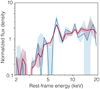 |
Fig. 19. Composite spectra of the seven Compton-thick AGN candidates selected by spectral fitting (blue) and 19 candidates filtered by the two X-ray colours, S/M and H/M, and R(Fe) alone (red). |
7.2. Evolution of the obscured AGN fraction
The distribution of absorbing column density, NH, of the whole sample has a median value of log NH = 22.5 [cm−2] (Fig. 3) and a shape similar to those obtained previously (e.g. Ueda et al. 2014; Liu et al. 2017). We note that this distribution has incompleteness originating from the bias against very Compton-thick AGN discussed in Sect. 4.1 and other various biases discussed in detail by Liu et al. (2017). AGN obscuration becomes higher at increasing redshifts: the NH distribution, obscured AGN fraction, X-ray colour analysis, and stacked spectra as a function of redshift all agree. Here, instead of the three redshift groups in Table 2, originally defined for the sake of spectral analysis, we rebin the redshifts into seven ranges, each of which contains a similar number of sources (24–30, except for 15 in the highest redshift range) and examine the obscured AGN fraction as a function of redshift (Fig. 20). The increasing trend of the obscured AGN fraction with increasing redshift agree with the study with the three redshift bins. The finer sampling of redshift suggests that there is perhaps a plateau between z = 1 and z = 2 and a steep increase at z > 2.5. In general, there is a bias for detection of absorption in higher redshift sources. However, in our spectral analysis, this bias was minimised by setting the same lower-bound rest-frame energy for all the spectra. Not only does the obscured AGN fraction, but also the median absorbing column also shows a similar increasing trend with redshift (Fig. 20).
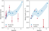 |
Fig. 20. Left: proportion of obscured AGN as a function of redshift. The blue squares show data for seven redshift ranges: 0.4–0.7, 0.7–1, 1–1.3, 1.3–1.6, 1.6–2, 2–2.6, and 2.6–3.8 in z. The 68% credible interval is indicated by the shaded area. The red filled circles are data for sources in the five redshift spikes. Right: median absorbing column density for the whole sample as a function of redshift. The shaded area indicates the 68% bootstrap error interval. The red symbols show the values for the five redshift spikes. |
The AGN obscured fraction is known to be luminosity dependent and decreases towards higher luminosity (e.g. Gilli et al. 2007; Ueda et al. 2014). For our sample, sources in higher redshift groups have, on average, larger luminosity as a result of the survey sensitivity limit. Therefore, under a hypothesis of no evolution of obscured AGN fraction, a decreasing trend of obscured fraction would be observed in XMM-CDFS. This was verified against the mock AGN catalogue5 produced by the AGN population model by Gilli et al. (2007) where a constant obscured fraction and the luminosity dependence are assumed. Observing the opposite trend over redshift supports the credibility of the increasing obscured fraction towards high redshift. This evolution of obscured AGN fraction has been suggested previously by a number of works (La Franca et al. 2005; Treister & Urry 2006; Hasinger 2008; Ebrero et al. 2009; Iwasawa et al. 2012a; Ueda et al. 2014; Liu et al. 2017; Vito et al. 2018) and it appears to be luminosity dependent (Buchner et al. 2015; Georgakakis et al. 2015; Aird et al. 2015).
7.3. Sources in redshift spikes
A few redshift spikes in the CDFS have been observed through optical spectroscopic surveys (e.g. Gilli et al. 2003; Silverman et al. 2010). We identified five redshift spikes composed of XMM-CDFS X-ray sources in our sample. Since our sample size is not large, they may easily be missed in a histogram like Fig. 1 due to the binning bias. A cumulative distribution function (CDF) is instead free from the binning bias. The CDF around the five redshift-spikes are shown in Fig. 21, in which a steep rise of the CDF is identified with each spike. These spikes have between six and 12 sources within Δz ≤ 0.03, respectively (Table 10). Each of them has a counterpart found by optical spectroscopy of galaxies in the field (e.g. Silverman et al. 2010). The total number of sources in these spikes is 45, in which three sources have photometric redshifts. The median properties of the sources belonging to each redshift spike are presented in Table 10.
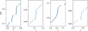 |
Fig. 21. Cumulative distribution function (CDF) of the XMM-CDFS source redshifts in the four redshift ranges, where the five redshift spikes at z ≃ 0.67, z ≃ 0.73, z = 1.22, z = 1.62, z ≃ 2.57 are found. A steep rise in CDF represets a redshift clustering. The two spikes at z ≃ 0.67 and z ≃ 0.73 are well separated in the first figure. |
X-ray source properties of redshift spikes.
As noted above, obscured AGN seem to be more abundant towards higher redshift and the sources in the three, lower redshift spikes (z = 0.67, 0.73 and 1.22) follow the same trend (Fig. 20). However, those in the two, higher redshift spikes (z = 1.61 and 2.57) deviate from this trend and show lower obscured AGN fractions and lower absorbing columns (Table 10). This behaviour is illustrated by the composite spectra of the sources in Fig. 22. The composite spectrum of the lower-z spikes is relatively hard (α = 0.56 ± 0.06, NH = (1.8 ± 0.5)×1022 cm−2) and agrees with that of the whole sample. In contrast, that of the higher-z spikes is clearly softer (α = 0.80 ± 0.05, NH = (5 ± 4)×1021 cm−2). Both spectra show Fe K lines with EW ≃ 0.1 keV. We note that the higher-z spikes composite spectrum shows an asymmetric Fe line profile with a red wing extending down to 5 keV. If the diskline model (Fabian et al. 1989) is fitted, the line EW would increase to 0.25 ± 0.02 keV.
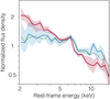 |
Fig. 22. Composite spectra for the three z-spikes in lower redshifts (blue, z ≃ 0.67, z ≃ 0.73, z ≃ 1.22) and in higher redshifts (red, z ≃ 1.61 and z ≃ 2.57). The composite spectrum of the whole sample is also plotted in green for comparison. While the spectrum of the low-z spikes agrees with that of the whole sample, the spectrum of the high-z spikes is clearly softer. |
The deficit of obscured AGN in the z = 1.61 and z = 2.57 spikes is puzzling. Since they are X-ray selected sources, there is little bias for unobscured AGN, which would be likely to occur in an optical spectroscopic selection. Indeed, the sources in the lower-z spikes show no difference in obscuration from the sources in the similar redshift range. It could be related to deficiency of gas in the nuclear regions or in the host galaxies. Faster gas consumption by star formation taking place earlier or faster transition of obscured to unobscured AGN by expelling, for example, the surrounding gas (Sanders et al. 1988), relative to the other sources, may provide an explanation. Whether this can be attributed to an environmental effect is uncertain. They are likely to be located in large-scale structures (Gilli et al. 2003) but their environments are not as dense as in a galaxy cluster. Gas removal by ram pressure stripping (etc.) should not be as efficient as in a more dense environment. A study of general galaxy properties in these redshift spikes, for example, of post-starburst proportions, may provide a clue for understanding the apparent deficit of obscuration.
7.4. Fe K emission lines
Fe K lines are frequently found in the spectra. The line energy is most frequently found at around 6.4 keV, indicating the majority of AGN emit cold Fe K lines. For the narrow component of the Fe K line in unobscured AGN, the Iwasawa-Taniguchi (IT) effect is well established among the nearby AGN (Bianchi et al. 2007; Page et al. 2004; Shu et al. 2012). The correlation is often interpreted as the consequence of decreasing torus covering factor with increasing source luminosity, as in Ricci et al. (2013). On the contrary, as far as the composite spectra are concerned, the XMM-CDFS sources show no luminosity dependence of the line EW. Furthermore, the observed EW around 0.1 keV seen in high-luminosity sources is well above the value predicted from the correlation (Fig. 16). However, this may not be surprising given that the XMM-CDFS sources are sampled over a wide redshift range. Statistically, larger luminosity sources come from higher redshifts. As discussed in the previous section for the whole sample, there is an evolution of obscuration of AGN, that is, more obscuration at higher redshifts. This could result from a larger gas mass fraction at higher redshifts (e.g. Carilli & Walter 2013) as discussed in Iwasawa et al. (2012a). The increased obscuration for higher redshift sources (hence higher luminosity sources on average) then means more cold gas surrounding the AGN regardless of their types (obscured or unobscured in the line-of sight). It would offset the decline of line intensity due to whatever mechanism produces the IT effect by providing more cold gas to be illuminated by the central source for the line production. The evolution of the gas fraction fgas ∝ (1 + z)2 (Geach et al. 2011) means an increase of ∼0.5 dex of cold gas from z = 0.7 to z = 2, which roughly matches the required offset. Chaudhary et al. (2010) found the IT effect in the AGN sample of the serendipitous 2XMM catalog (Watson et al. 2009), which includes sources with redshifts up to z ∼ 5, using spectral stacking. We note that since their sample is dominated by low redshift objects, the IT effect is probably driven by sources in the limited, low redshift range.
Substantial line broadening of Fe K emission, most likely due to the relativistic effects at inner radii of the accretion disc, in distant AGN have been studied by many authors using spectral stacking (Streblyanska et al. 2005; Brusa et al. 2005; Corral et al. 2008; Chaudhary et al. 2012; Iwasawa et al. 2012b; Falocco et al. 2013, 2014). Results vary between the works but some evidence of line broadening has been found. We observe a 30% of detection rate of line broadening with σ ≥ 0.3 keV among the bright, individual unobscured sources in the XMM-CDFS (Sect. 4.3.2), which is similar to that for nearby AGN (de La Calle Pérez et al. 2010). The lack of strong line broadening in our composite spectrum of all the unobscured AGN (see also Falocco et al. 2013) suggests that broad Fe K lines in distant AGN are not much more common than in the local AGN.
However, when we have a limited signal-to-noise ratio for spectral data, a relativistically broadened line could escape from detection. The archetypal broad Fe line shape (Tanaka et al. 1995), as with, for example, the disc inclination of ∼30°, the inner radius of 6rg, would be the easiest to detect with the spectral resolution of a CCD detector. What we are looking to examine is specifically this type of line broadening. Under more extreme relativistic effects, line emission is altered to become so broad and its contrast against the continuum is so low that its detection is deemed to be difficult. Presence of a narrow line component originating from distant matter makes it even more complicated.
sne310 can be found in the electronic form of Table 1.
Acknowledgments
This research made use of data obtained from XMM-Newton and software packages of HEASoft, R (Core 2017), rjags, ggplot2 (Wickham 2009), IPython (Pérez & Granger 2007), and Matplotlib (Hunter 2007). We acknowledge financial contribution from the agreement ASI-INAF n.2017-14-H.O. KI acknowledges support by the Spanish MINECO under grant AYA2016-76012-C3-1-P and MDM-2014-0369 of ICCUB (Unidad de Excelencia “María de Maeztu”). AC acknowledges the Caltech Kingsley visitor program. FJC acknowledges financial support through grant AYA2015-64346-C2-1P (MINECO/FEDER), by the Spanish Ministry MCIU under project RTI2018-096686-B-C21 (MCIU/AEI/FEDER, UE), cofunded by FEDER funds, and funded by the Agencia Estatal de Investigación, Unidad de Excelencia María de Maeztu, MDM-2017-0765. WNB acknowledges support from NASA grants 80NSSC19K0961 and 80NSSC18K0878.
References
- Aird, J., Coil, A. L., Georgakakis, A., et al. 2015, MNRAS, 451, 1892 [NASA ADS] [CrossRef] [Google Scholar]
- Akylas, A., Georgakakis, A., Georgantopoulos, I., Brightman, M., & Nandra, K. 2012, A&A, 546, A98 [NASA ADS] [CrossRef] [EDP Sciences] [Google Scholar]
- Ananna, T. T., Treister, E., Urry, C. M., et al. 2019, A&A, 871, 240 [Google Scholar]
- Antonucci, M., Talavera, A., Vagnetti, F., et al. 2015, A&A, 574, A49 [NASA ADS] [CrossRef] [EDP Sciences] [Google Scholar]
- Balestra, I., Mainieri, V., Popesso, P., et al. 2010, A&A, 512, A12 [NASA ADS] [CrossRef] [EDP Sciences] [Google Scholar]
- Ballantyne, D. R., Draper, A. R., Madsen, K. K., Rigby, J. R., & Treister, E. 2011, A&A, 736, 56 [Google Scholar]
- Bianchi, S., Guainazzi, M., Matt, G., & Fonseca Bonilla, N. 2007, A&A, 467, L19 [NASA ADS] [CrossRef] [EDP Sciences] [Google Scholar]
- Bianchi, S., Guainazzi, M., Matt, G., Fonseca Bonilla, N., & Ponti, G. 2009, A&A, 495, 421 [NASA ADS] [CrossRef] [EDP Sciences] [Google Scholar]
- Bonzini, M., Padovani, P., Mainieri, V., et al. 2013, MNRAS, 436, 3759 [NASA ADS] [CrossRef] [Google Scholar]
- Brandt, W. N., & Alexander, D. M. 2015, A&ARv, 23, 1 [Google Scholar]
- Brandt, W. N., & Hasinger, G. 2005, ARA&A, 43, 827 [Google Scholar]
- Brightman, M., & Ueda, Y. 2012, MNRAS, 423, 702 [NASA ADS] [CrossRef] [Google Scholar]
- Brusa, M., Gilli, R., & Comastri, A. 2005, ApJ, 621, L5 [NASA ADS] [CrossRef] [Google Scholar]
- Buchner, J., Georgakakis, A., Nandra, K., et al. 2015, A&A, 802, 89 [Google Scholar]
- Burlon, D., Ajello, M., Greiner, J., et al. 2011, A&A, 728, 58 [Google Scholar]
- Cardamone, C. N., van Dokkum, P. G., Urry, C. M., et al. 2010, ApJS, 189, 270 [NASA ADS] [CrossRef] [Google Scholar]
- Carilli, C. L., & Walter, F. 2013, ARA&A, 51, 105 [NASA ADS] [CrossRef] [EDP Sciences] [Google Scholar]
- Casey, C. M., Chapman, S. C., Smail, I., et al. 2011, MNRAS, 411, 2739 [NASA ADS] [CrossRef] [Google Scholar]
- Castelló-Mor, N., Carrera, F. J., Alonso-Herrero, A., et al. 2013, A&A, 556, A114 [NASA ADS] [CrossRef] [EDP Sciences] [Google Scholar]
- Chaudhary, P., Brusa, M., Hasinger, G., Merloni, A., & Comastri, A. 2010, A&A, 518, A58 [NASA ADS] [CrossRef] [EDP Sciences] [Google Scholar]
- Chaudhary, P., Brusa, M., Hasinger, G., et al. 2012, A&A, 537, A6 [NASA ADS] [CrossRef] [EDP Sciences] [Google Scholar]
- Comastri, A., Ranalli, P., Iwasawa, K., et al. 2011, A&A, 526, L9 [NASA ADS] [CrossRef] [EDP Sciences] [Google Scholar]
- Cooper, M. C., Yan, R., Dickinson, M., et al. 2012, MNRAS, 425, 2116 [NASA ADS] [CrossRef] [Google Scholar]
- Corral, A., Page, M. J., Carrera, F. J., et al. 2008, A&A, 492, 71 [NASA ADS] [CrossRef] [EDP Sciences] [Google Scholar]
- de La Calle Pérez, I., Longinotti, A. L., Guainazzi, M., et al. 2010, A&A, 524, A50 [NASA ADS] [CrossRef] [EDP Sciences] [Google Scholar]
- Dickey, J. M., & Lockman, F. J. 1990, ARA&A, 28, 215 [NASA ADS] [CrossRef] [MathSciNet] [Google Scholar]
- Ebrero, J., Carrera, F. J., Page, M. J., et al. 2009, A&A, 493, 55 [NASA ADS] [CrossRef] [EDP Sciences] [Google Scholar]
- Efron, B. 1979, Ann. Stat., 7, 1 [Google Scholar]
- Fabian, A. C., Rees, M. J., Stella, L., & White, N. E. 1989, MNRAS, 238, 729 [NASA ADS] [CrossRef] [Google Scholar]
- Fabian, A. C., Iwasawa, K., Reynolds, C. S., & Young, A. J. 2000, PASP, 112, 1145 [NASA ADS] [CrossRef] [Google Scholar]
- Falocco, S., Carrera, F. J., Corral, A., et al. 2013, A&A, 555, A79 [NASA ADS] [CrossRef] [EDP Sciences] [Google Scholar]
- Falocco, S., Carrera, F. J., Barcons, X., Miniutti, G., & Corral, A. 2014, A&A, 568, A15 [CrossRef] [EDP Sciences] [Google Scholar]
- Falocco, S., Paolillo, M., Comastri, A., et al. 2017, A&A, 608, A32 [CrossRef] [EDP Sciences] [Google Scholar]
- Geach, J. E., Smail, I., Moran, S. M., et al. 2011, ApJ, 730, L19 [NASA ADS] [CrossRef] [Google Scholar]
- Georgakakis, A., Aird, J., Buchner, J., et al. 2015, MNRAS, 453, 1946 [Google Scholar]
- Georgantopoulos, I., Comastri, A., Vignali, C., et al. 2013, A&A, 555, A43 [NASA ADS] [CrossRef] [EDP Sciences] [Google Scholar]
- Giacconi, R., Rosati, P., Tozzi, P., et al. 2001, A&A, 551, 624 [Google Scholar]
- Gilli, R., Cimatti, A., Daddi, E., et al. 2003, A&A, 592, 721 [Google Scholar]
- Gilli, R., Comastri, A., & Hasinger, G. 2007, A&A, 463, 79 [NASA ADS] [CrossRef] [EDP Sciences] [Google Scholar]
- Hales, C. A., Norris, R. P., Gaensler, B. M., et al. 2014, MNRAS, 441, 2555 [NASA ADS] [CrossRef] [Google Scholar]
- Hasinger, G. 2008, A&A, 490, 905 [NASA ADS] [CrossRef] [EDP Sciences] [Google Scholar]
- Hsu, L.-T., Salvato, M., Nandra, K., et al. 2014, A&A, 796, 60 [Google Scholar]
- Hunter, J. D. 2007, Comput. Sci. Eng., 9, 90 [NASA ADS] [CrossRef] [Google Scholar]
- Huynh, M. T., Bell, M. E., Hopkins, A. M., Norris, R. P., & Seymour, N. 2015, MNRAS, 454, 952 [NASA ADS] [CrossRef] [Google Scholar]
- Ikeda, S., Awaki, H., & Terashima, Y. 2009, A&A, 692, 608 [Google Scholar]
- Iwasawa, K., & Taniguchi, Y. 1993, ApJ, 413, L15 [NASA ADS] [CrossRef] [Google Scholar]
- Iwasawa, K., Gilli, R., Vignali, C., et al. 2012a, A&A, 546, A84 [NASA ADS] [CrossRef] [EDP Sciences] [Google Scholar]
- Iwasawa, K., Mainieri, V., Brusa, M., et al. 2012b, A&A, 537, A86 [NASA ADS] [CrossRef] [EDP Sciences] [Google Scholar]
- Iwasawa, K., Vignali, C., Comastri, A., et al. 2015, A&A, 574, A144 [NASA ADS] [CrossRef] [EDP Sciences] [Google Scholar]
- Kellermann, K. I., Sramek, R., Schmidt, M., Shaffer, D. B., & Green, R. 1989, AJ, 98, 1195 [NASA ADS] [CrossRef] [Google Scholar]
- Komatsu, E., Smith, K. M., Dunkley, J., et al. 2011, ApJS, 192, 18 [NASA ADS] [CrossRef] [Google Scholar]
- Koss, M. J., Assef, R., Baloković, M., et al. 2016, A&A, 825, A85 [Google Scholar]
- Kurk, J., Cimatti, A., Daddi, E., et al. 2013, A&A, 549, A63 [NASA ADS] [CrossRef] [EDP Sciences] [Google Scholar]
- La Franca, F., Fiore, F., Comastri, A., et al. 2005, A&A, 635, 864 [Google Scholar]
- Lambrides, E., Chiaberge, M., Heckman, T., et al. 2020, ApJ, submitted [arXiv:2002.00955] [Google Scholar]
- Lanzuisi, G., Civano, F., Marchesi, S., et al. 2018, MNRAS, 480, 2578 [NASA ADS] [CrossRef] [Google Scholar]
- Le Fèvre, O., Cassata, P., Cucciati, O., et al. 2013, A&A, 559, A14 [NASA ADS] [CrossRef] [EDP Sciences] [Google Scholar]
- Liu, T., Tozzi, P., Wang, J.-X., et al. 2017, ApJS, 232, 8 [NASA ADS] [CrossRef] [Google Scholar]
- Luo, B., Brandt, W. N., Xue, Y. Q., et al. 2010, ApJS, 187, 560 [NASA ADS] [CrossRef] [Google Scholar]
- Luo, B., Brandt, W. N., Xue, Y. Q., et al. 2017, ApJS, 228, 2 [Google Scholar]
- Masini, A., Civano, F., Comastri, A., et al. 2018, ApJS, 235, 17 [NASA ADS] [CrossRef] [Google Scholar]
- Mignoli, M., Pozzetti, L., Comastri, A., et al. 2004, A&A, 418, 827 [NASA ADS] [CrossRef] [EDP Sciences] [Google Scholar]
- Mignoli, M., Cimatti, A., Zamorani, G., et al. 2005, A&A, 437, 883 [NASA ADS] [CrossRef] [EDP Sciences] [Google Scholar]
- Morris, A. M., Kocevski, D. D., Trump, J. R., et al. 2015, AJ, 149, 178 [NASA ADS] [CrossRef] [Google Scholar]
- Nandra, K., & Pounds, K. A. 1994, MNRAS, 268, 405 [NASA ADS] [CrossRef] [Google Scholar]
- Norman, C., Hasinger, G., Giacconi, R., et al. 2002, A&A, 571, 218 [Google Scholar]
- Padovani, P., Miller, N., Kellermann, K. I., et al. 2011, A&A, 740, 20 [Google Scholar]
- Page, K. L., O’Brien, P. T., Reeves, J. N., & Turner, M. J. L. 2004, MNRAS, 347, 316 [NASA ADS] [CrossRef] [Google Scholar]
- Pentericci, L., McLure, R. J., Franzetti, P., Garilli, B., & the VANDELS team 2018, ArXiv e-prints [arXiv:1811.05298] [Google Scholar]
- Pérez, F., & Granger, B. E. 2007, Comput. Sci. Eng., 9, 21 [Google Scholar]
- Popesso, P., Dickinson, M., Nonino, M., et al. 2009, A&A, 494, 443 [NASA ADS] [CrossRef] [EDP Sciences] [Google Scholar]
- Core, R., & Team., 2017, R: A Language and Environment for Statistical Computing (Vienna, Austria: R Foundation for Statistical Computing) [Google Scholar]
- Rafferty, D. A., Brandt, W. N., Alexander, D. M., et al. 2011, A&A, 742, A3 [Google Scholar]
- Ranalli, P., Comastri, A., Vignali, C., et al. 2013, A&A, 555, A42 [NASA ADS] [CrossRef] [EDP Sciences] [Google Scholar]
- Ravikumar, C. D., Puech, M., Flores, H., et al. 2007, A&A, 465, 1099 [NASA ADS] [CrossRef] [EDP Sciences] [Google Scholar]
- Ricci, C., Paltani, S., Awaki, H., et al. 2013, A&A, 553, A29 [NASA ADS] [CrossRef] [EDP Sciences] [Google Scholar]
- Ricci, C., Ueda, Y., Koss, M. J., et al. 2015, ApJ, 815, L13 [NASA ADS] [CrossRef] [Google Scholar]
- Sanders, D. B., Soifer, B. T., Elias, J. H., et al. 1988, A&A, 325, 74 [Google Scholar]
- Shu, X. W., Wang, J. X., Yaqoob, T., Jiang, P., & Zhou, Y. Y. 2012, ApJ, 744, L21 [NASA ADS] [CrossRef] [Google Scholar]
- Silverman, J. D., Mainieri, V., Salvato, M., et al. 2010, ApJS, 191, 124 [NASA ADS] [CrossRef] [Google Scholar]
- Straatman, C. M. S., Spitler, L. R., Quadri, R. F., et al. 2016, A&A, 830, A51 [Google Scholar]
- Streblyanska, A., Hasinger, G., Finoguenov, A., et al. 2005, A&A, 432, 395 [NASA ADS] [CrossRef] [EDP Sciences] [Google Scholar]
- Strüder, L., Briel, U., Dennerl, K., et al. 2001, A&A, 365, L18 [NASA ADS] [CrossRef] [EDP Sciences] [Google Scholar]
- Szokoly, G. P., Bergeron, J., Hasinger, G., et al. 2004, ApJS, 155, 271 [NASA ADS] [CrossRef] [Google Scholar]
- Tanaka, Y., Nandra, K., Fabian, A. C., et al. 1995, Nature, 375, 659 [NASA ADS] [CrossRef] [Google Scholar]
- Taylor, E. N., Franx, M., van Dokkum, P. G., et al. 2009, ApJS, 183, 295 [NASA ADS] [CrossRef] [Google Scholar]
- Tozzi, P., Gilli, R., Mainieri, V., et al. 2006, A&A, 451, 457 [NASA ADS] [CrossRef] [EDP Sciences] [Google Scholar]
- Treister, E., & Urry, C. M. 2006, ApJ, 652, L79 [NASA ADS] [CrossRef] [Google Scholar]
- Treister, E., Virani, S., Gawiser, E., et al. 2009, A&A, 693, 1713 [Google Scholar]
- Turner, M. J. L., Abbey, A., Arnaud, M., et al. 2001, A&A, 365, L27 [NASA ADS] [CrossRef] [EDP Sciences] [Google Scholar]
- Ueda, Y., Akiyama, M., Hasinger, G., Miyaji, T., & Watson, M. G. 2014, A&A, 786, A104 [Google Scholar]
- Urrutia, T., Wisotzki, L., Kerutt, J., et al. 2019, A&A, 624, A141 [NASA ADS] [CrossRef] [EDP Sciences] [Google Scholar]
- Vanzella, E., Cristiani, S., Dickinson, M., et al. 2008, A&A, 478, 83 [NASA ADS] [CrossRef] [EDP Sciences] [Google Scholar]
- Vignali, C., Iwasawa, K., Comastri, A., et al. 2015, A&A, 583, A141 [NASA ADS] [CrossRef] [EDP Sciences] [Google Scholar]
- Vito, F., Brandt, W. N., Yang, G., et al. 2018, MNRAS, 473, 2378 [NASA ADS] [CrossRef] [Google Scholar]
- Watson, M. G., Schröder, A. C., Fyfe, D., et al. 2009, A&A, 493, 339 [NASA ADS] [CrossRef] [EDP Sciences] [Google Scholar]
- Wickham, H. 2009, ggplot2: Elegant Graphics for Data Analysis (New York: Springer-Verlag) [Google Scholar]
- Xue, Y. Q., Luo, B., Brandt, W. N., et al. 2016, ApJS, 224, 15 [NASA ADS] [CrossRef] [Google Scholar]
Appendix A: X-ray redshifts
Table A.1 lists 11 sources for which no spectroscopic redshifts are available and, instead, redshifts are obtained from X-ray Fe K band spectral measurements, in addition to the six sources with redshifts derived by the same technique and published previously (Iwasawa et al. 2012a; Vignali et al. 2015). Seven sources out of 11 are strongly absorbed by log NH ≥ 23 [cm−2] (see Table 1) and the redshift estimates are driven by the Fe K absorption edge. When a Fe K line, compatible with the estimate by the absorption edge, is detected, the redshift and its uncertainty are revised. Existing photometric redshifts were used as a guide and if an X-ray estimate was better constrained, we adopted the X-ray redshift. Photometric redshifts of these sources are all available from Hsu et al. (2014) (H14 hereafter), they are shown in Table A.1 for reference. Further comments on three sources marked in the Table are given below.
11 sources with X-ray redshift estimates.
PID 88: This X-ray redshift is a tentative assignment, as there is no agreement between the insecure spectroscopic (z = 0.522), the two equally likely photometric redshifts by H14 given in the table (the probability density function for the photometric redshift shows a double peaks with comparable heights) and the X-ray estimate. A strong line feature at 3 keV is identified as a Fe K line to estimate the redshift but it might be a false detection given the relatively soft spectrum. Therefore, any of the redshift estimates are highly uncertain.
PID 166: The X-ray spectrum of this source is strongly absorbed with log NH = 23.18 [cm−2]. H14 gives a mild constraint on zph = 1.688 while Straatman et al. (2016) gives zph = 1.377. A combination of the Fe K edge and Fe K line gives the reasonably constrained zx close to the estimate of Straatman et al. (2016).
PID 215: Two Chandra sources are present at the XMM source position (Luo et al. 2017). The fainter source has a spectroscopic redshift of z = 2.252 (Casey et al. 2011) while the brighter source (which is fainter in optical/NIR) has photometric redshift estimates by H14 and zph = 2.6 by Straatman et al. (2016). The XMM spectrum of this source shows a strong Fe K line feature at 1.75 keV, which is compatible with the photometric redshift for the brighter Chandra source. The strong Fe line and the hard continuum make this source as a likely Compton-thick AGN.
Appendix B: Examples of Fe K band continuum estimate
In Sect. 5.2, how the Fe K band continuum flux in each spectrum of the uniform rest-frame intervals is outlined. We describe here supplemental details on the method and a few examples of its application.
First, we pick 10 spectral bins below and above the Fe K bin (i = 13, which is excluded from this analysis) so that we have 5 bins on each side. The lower 5 bins ranges from 4.0 keV to 6.0 keV (i = 8–12) while the higher from 6.6 keV to 10 keV (i= 14–18). The central bins on the two bands are at 4.9 keV (i = 10) and 8.2 keV (i = 16), respectively. In each spectrum, we take a median of each band and adopt the median value as the flux density of the central bin of each band.

where fi represents flux density at i-th channel while  is “estimated” continuum flux density at the given channel.
  (or
(or  ) may coincide with f10 (or f16) but it could be a value measured at the other bin, which holds the median value. Thus we have two continuum estimates at i = 10 and i = 16. Taking a logarithmic mean of the two gives an estimate of the continuum at i = 13, because all the bins are logarithmically equal intervals by design.
where  is the estimated continuum flux density at i = 13, the Fe K band (6.0–6.6 keV).
When, for example, a continuum shape is a simple power-law and data quality is good, there is no complication in obtaining f′ at i = 10 and i = 16 and they are usually equal to f10 and f16. However, when you have noisy data (which is often the case for XMM-CDFS sources), data deviate from the underlying continuum shape and spectral fitting is an usual solution. The above operation using the median statistic, however, seems to give a reasonable estimate of the two continuum data points encompassing the Fe K band and the resulted Fe K band continuum flux, as supported by the intercept of Fig. 11 being very close to 1. Even when an Fe K line is not found at i = 13 but at the other interval, the median estimate remains robust.
Figure B.1 shows examples of applying this method, for a good quality spectrum (PID 203) and a noisy spectrum (PID 323). For PID 203,  and
and  . On the other hand, for PID 323, the median values in both lower and higher energy bands occur at intervals different from the respective central energy intervals, hence
  and
and  are assigned to estimate
  , as indicated in the figure.
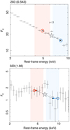 |
Fig. B.1. Examples of Fe K continuum estimates for PID 203 and PID 323. A value inside the parenthesis following the PID in each figure is adopted source redshift. The shaded areas indicate the lower and higher energy ranges encompassing the Fe K band. The open circles indicate where the median values are found in the respective energy ranges. The dotted line is an adopted continuum between the 4.9 keV (i = 10) and 8.2 keV (i = 16) with the estimated continuum level at i = 13 (open star). |
Appendix C: Median/mean stacking for a composite spectrum
While previous X-ray spectral stacking work normally use mean stacking of normalised spectra (or a straight sum), we use median stacking to construct a composite spectrum, which is a normal practice in UV/optical/infrared spectroscopy. Median statistic is relatively robust against outliers and a skewed distribution, compared to mean statistic. We offer a few examples to illustrate why median stacking might perform better in obtaining a typical spectral shape than mean stacking, at least for our dataset. Fig. C.1 shows the cumulative distribution function (CDF) of three spectral channels of i = 4, i = 13 and i = 17, corresponding to the rest-frame 3 keV, 6.3 keV and 9 keV, respectively, of the 180 sources to construct the composite spectra in Fig. C.2. The CDF for i = 4 reasonably follows the normal distribution and the mean and median statistics remain close. The i = 13 CDF is skewed towards high values with outliers, as expected from the skewed EW distribution (Fig. 5) and the presence of a few very strong Fe K line sources. This stretches the fitted normal distribution wider and drags it to higher values. The resulted mean is 1.51, while the median is 1.27. This difference is translated to a factor of ∼2 larger EW of the Fe line in the mean stacking than in the median stacking spectrum, as seen in Fig. C.2. Judging from the CDF, the median appears more representative than the mean in this particular channel. The i = 17 CDF is closer to a symmetric shape but outliers make the fitted normal distribution incompatible to the data. Since our X-ray data of faint sources are noisy, each spectral channel often contains some outliers. In terms of describing the distribution, a t-distribution, which has an extra parameter for heavier distribution tails, could be a solution. In fact, a t-distribution gives a good description of the CDF of i = 17 and of many other channels (i = 13 is a notable exception but the central value, 1.29, is much closer to the median than the mean is). However, for the simplicity and robustness of median statistic, we opted to use median stacking to look for typical spectral shape for our dataset.
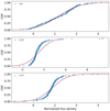 |
Fig. C.1. CDF of normalised flux density values (blue crosses) of the 180 XMM-CDFS sources in three spectral channels, i = 4, i = 13, i = 17, corresponding to the rest frame energies, 3 keV, 6.3 keV (Fe K band), and 9 keV, respectively. A theoretical curve of the normal distribution which fits the data is overplotted in red in each plot. |
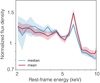 |
Fig. C.2. Composite spectra of all the 180 XMM-CDFS sources at z > 0.4, constructed by median (blue) and mean (red) stacking. The composite spectrum of Fig. 12 in the main text is identical to that of median stacking. |
Appendix D: XMM-CDFS EPIC spectral atlas
The remaining 182 spectra of Fig. 2 are shown in Fig. D.1.
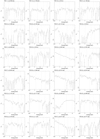 |
Fig. D.1. Observed 0.5–7 keV spectra of the remaining 182 XMM-CDFS sources of Fig. 2. Flux density is in units of 10−15 erg s−1 cm−2 keV−1. The energy scale is as observed and the three, vertical dotted lines indicate the rest-frame energies of 3 keV, 6.4 keV and 10 keV, expected from the adopted redshift. |
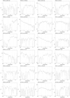 |
Fig. D.1. continued. |
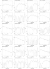 |
Fig. D.1. continued. |
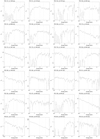 |
Fig. D.1. continued. |
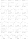 |
Fig. D.1. continued. |
 |
Fig. D.1. continued. |
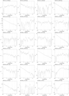 |
Fig. D.1. continued. |
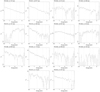 |
Fig. D.1. continued. |
All Tables
Median properties of sources in the three redshift ranges and three redshift estimate types.
All Figures
|
Fig. 1. Redshift distribution of the 185 XMM-CDFS sources (blue). The majority are spectroscopic redshifts. Photometric redshifts and X-ray redshifts are overdrawn in red and green, respectively. The redshift ranges of lowz, midz and highz are labeled and their boundaries are marked by dashed lines. |
| In the text | |
|
Fig. 2. Observed 0.5–7 keV spectra of 185 XMM-CDFS sources, shown in order of PID number. Only the first three spectra are shown here and the remaining 182 spectra can be found in Appendix D. Flux density is in units of 10−15 erg s−1 cm−2 keV−1. The energy scale is as observed and the three, vertical dotted lines indicate the rest-frame energies of 3 keV, 6.4 keV and 10 keV, expected from the adopted redshift. |
| In the text | |
|
Fig. 3. Upper panel: distribution of best-fit NH values obtained for all the 180 sources at z > 0.4. The histogram in red shows the NH distribution of absorption detected sources, while the blue histogram shows that of the upper limits. We note the limited but uniform sensitivity of our spectra to NH due to the rest-frame bandpass (see text). Lower panel: box-and-whisker plots of NH measurements for the lowz, midz and highz groups. Following the normal convention, the box represents the inter quatile range (the middle 50%), the bar in the middle represents the median value, and the whiskers show the range of the minimum and the maximum of the distribution. |
| In the text | |
|
Fig. 4. Rest-frame 2–10 keV luminosity distributions for all the 180 sources, the lowz, midz and highz sources. The solid line histograms denote the distribution of absorption-corrected luminosity, while the dotted lines are for luminosity as observed. |
| In the text | |
|
Fig. 5. Main: Fe K line equivalent width distributions of the 71 sources with the line detection at the 90% significance. Inset: the same distribution for the lines of the 68% line detection (red) and that for the upper limits of no detection (green). |
| In the text | |
|
Fig. 6. Spectral data of six unobscured sources exhibiting broad Fe K features. The data are divided by the best-fit power-law. The source identification number is indicated. The upper four sources come from the lowz group while the lower two from the highz group (see Fig. 8). |
| In the text | |
|
Fig. 7. Stacked spectra of the six broad Fe-line AGN (a) and the other 15 AGN (b) of the 21 unobscured sources with highest quality data. |
| In the text | |
|
Fig. 8. Cumulative distribution functions of the redshifts of the 21 unobscured AGN with good data quality (blue circles) and those of the six in which broad Fe lines are detected (red squares). The redshifts of the sample AGN are spread over the range of 0.5–2.6 with some clustering in the z = 1.6–2 range. In contrast, broad line detections may be frequent at low redshifts (z < 0.9). |
| In the text | |
|
Fig. 9. S/M colours against best-fitting NH, obtained from the conventional spectral fit. The dashed line indicates the best-fitting relation in the range of 22–23.3 in log NH [cm−2] (see text). |
| In the text | |
|
Fig. 10. Colour–colour (H/M – S/M) diagram for the midz and highz sources. The locus in dashed red line indicates the evolution of (S/M, H/M) when a power-law continuum of energy index α = 0.8 is modified by cold absorption with various column densities: log NH [cm−2] of 22, 22.5, 23, 23.5, 23.7, 23.85 and 24, as marked by cross symbols. Colours for a simple power-law with no absorption with α of 0.8, 1.0, and 1.2 are also marked. |
| In the text | |
|
Fig. 11. Left: Fe K line strength indicator, R(Fe), against the Fe K line equivalent width (EW) obtained from spectral fitting. The filled squares (red) show data for Fe lines with the ≥90% detection while the circles (light blue) show data for weak/no detection for the whole sample. The dashed line indicates the fitted linear correlation (see text). The dotted line indicates the expected relation when the continuum level estimate of the i = 13 bin is accurate. Right: same plot for the crowded region of EW < 0.8 keV. |
| In the text | |
|
Fig. 12. Upper panel: rest-frame 2–20 keV composite spectrum of all the 180 sources at 0.4 < z < 3.8. The shaded area indicates 68% confidence intervals from bootstrap. Lower panel: same spectra for the lowz, midz and highz sources. |
| In the text | |
|
Fig. 13. S/M X-ray colour distributions of lowz, midz, and highz groups. |
| In the text | |
|
Fig. 14. Composite spectra of sources with spectroscopic redshifts and and photometric redshift estimates. |
| In the text | |
|
Fig. 15. Left panel: composite spectrum of all the 81 unobscured AGN with the best-fit power-law plus a narrow Gaussian for the Fe K emission and the residual in ratio of the data and the model. Right panel: composite spectra of unobscured sources in the lowz, midz and highz groups. The spectra are plotted with arbitrary offsets for clarity. |
| In the text | |
|
Fig. 16. Narrow Fe K line EW against X-ray luminosity obtained from the three luminosity slices of unobscured AGN (Table 9). The dashed and dash-dotted lines indicate the I-T effect obtained for nearby AGN by Bianchi et al. (2007) and Shu et al. (2012), respectively. |
| In the text | |
|
Fig. 17. Probability distributions for the Compton-thick AGN fraction obtained from the XMM-CDFS (in blue) using the beta distribution prior (in red) which approximates the distribution of previous measurements for nearby AGN using hard X-ray instruments and Chandra CDFS measurements (references are given in text). The best estimate is found at 0.04 with the 95% credible interval of (0.024–0.078). |
| In the text | |
|
Fig. 18. Same X-ray colour-colour diagram as Fig. 10 with information of R(Fe) added by the symbol size (the larger the size, the larger the R(Fe) value), to illustrate the Compton-thick AGN selection by the X-ray colours and R(Fe) alone (without spectral fitting). The error bars of the X-ray colours are omitted for clarity. Sources with strong Fe K lines (EW ≥ 1 keV, measured by spectral fitting) are distinguished by colour. The seven Compton thick AGN candidates are marked by red triangles. Requiring S/M < 1.5 and H/M > 0.5 ensures a hard spectrum of a reflection-dominated source. |
| In the text | |
|
Fig. 19. Composite spectra of the seven Compton-thick AGN candidates selected by spectral fitting (blue) and 19 candidates filtered by the two X-ray colours, S/M and H/M, and R(Fe) alone (red). |
| In the text | |
|
Fig. 20. Left: proportion of obscured AGN as a function of redshift. The blue squares show data for seven redshift ranges: 0.4–0.7, 0.7–1, 1–1.3, 1.3–1.6, 1.6–2, 2–2.6, and 2.6–3.8 in z. The 68% credible interval is indicated by the shaded area. The red filled circles are data for sources in the five redshift spikes. Right: median absorbing column density for the whole sample as a function of redshift. The shaded area indicates the 68% bootstrap error interval. The red symbols show the values for the five redshift spikes. |
| In the text | |
|
Fig. 21. Cumulative distribution function (CDF) of the XMM-CDFS source redshifts in the four redshift ranges, where the five redshift spikes at z ≃ 0.67, z ≃ 0.73, z = 1.22, z = 1.62, z ≃ 2.57 are found. A steep rise in CDF represets a redshift clustering. The two spikes at z ≃ 0.67 and z ≃ 0.73 are well separated in the first figure. |
| In the text | |
|
Fig. 22. Composite spectra for the three z-spikes in lower redshifts (blue, z ≃ 0.67, z ≃ 0.73, z ≃ 1.22) and in higher redshifts (red, z ≃ 1.61 and z ≃ 2.57). The composite spectrum of the whole sample is also plotted in green for comparison. While the spectrum of the low-z spikes agrees with that of the whole sample, the spectrum of the high-z spikes is clearly softer. |
| In the text | |
|
Fig. B.1. Examples of Fe K continuum estimates for PID 203 and PID 323. A value inside the parenthesis following the PID in each figure is adopted source redshift. The shaded areas indicate the lower and higher energy ranges encompassing the Fe K band. The open circles indicate where the median values are found in the respective energy ranges. The dotted line is an adopted continuum between the 4.9 keV (i = 10) and 8.2 keV (i = 16) with the estimated continuum level at i = 13 (open star). |
| In the text | |
|
Fig. C.1. CDF of normalised flux density values (blue crosses) of the 180 XMM-CDFS sources in three spectral channels, i = 4, i = 13, i = 17, corresponding to the rest frame energies, 3 keV, 6.3 keV (Fe K band), and 9 keV, respectively. A theoretical curve of the normal distribution which fits the data is overplotted in red in each plot. |
| In the text | |
|
Fig. C.2. Composite spectra of all the 180 XMM-CDFS sources at z > 0.4, constructed by median (blue) and mean (red) stacking. The composite spectrum of Fig. 12 in the main text is identical to that of median stacking. |
| In the text | |
|
Fig. D.1. Observed 0.5–7 keV spectra of the remaining 182 XMM-CDFS sources of Fig. 2. Flux density is in units of 10−15 erg s−1 cm−2 keV−1. The energy scale is as observed and the three, vertical dotted lines indicate the rest-frame energies of 3 keV, 6.4 keV and 10 keV, expected from the adopted redshift. |
| In the text | |
|
Fig. D.1. continued. |
| In the text | |
|
Fig. D.1. continued. |
| In the text | |
|
Fig. D.1. continued. |
| In the text | |
|
Fig. D.1. continued. |
| In the text | |
|
Fig. D.1. continued. |
| In the text | |
|
Fig. D.1. continued. |
| In the text | |
|
Fig. D.1. continued. |
| In the text | |
Current usage metrics show cumulative count of Article Views (full-text article views including HTML views, PDF and ePub downloads, according to the available data) and Abstracts Views on Vision4Press platform.
Data correspond to usage on the plateform after 2015. The current usage metrics is available 48-96 hours after online publication and is updated daily on week days.
Initial download of the metrics may take a while.