| Issue |
A&A
Volume 638, June 2020
|
|
|---|---|---|
| Article Number | A114 | |
| Number of page(s) | 11 | |
| Section | Cosmology (including clusters of galaxies) | |
| DOI | https://doi.org/10.1051/0004-6361/201937283 | |
| Published online | 23 June 2020 | |
CODEX clusters
Survey, catalog, and cosmology of the X-ray luminosity function⋆
1
Department of Physics, University of Helsinki, Gustaf Hällströmin katu 2, 00014 Helsinki, Finland
e-mail: This email address is being protected from spambots. You need JavaScript enabled to view it.
2
Kavli Institute for Particle Astrophysics & Cosmology, PO Box 2450, Stanford University, Stanford, CA 94305, USA
3
SLAC National Accelerator Laboratory, Menlo Park, CA 94025, USA
4
IRAP, Université de Toulouse, CNRS, UPS, CNES, Toulouse, France
5
INAF-Osservatorio Astronomico di Trieste, Via G. B Tiepolo 11, 34143 Trieste, Italy
6
IFPU-Institute for Fundamental Physics of the Universe, Via Beirut 2, 34014 Trieste, Italy
7
Oskar Klein Centre, Department of Physics, Stockholm University, AlbaNova University Centre, 106 91 Stockholm, Sweden
8
Max Planck Institute for Extraterrestrial Physics, Giessenbachstrasse, 85748 Garching, Germany
9
Observatório Nacional, Ministério da Ciência, Tecnologia, Inovação e Comunicações, Rua General José Cristino, 77, São Cristão, 20921-400 Rio de Janeiro, RJ, Brazil
10
Institute for Astronomy, 2680 Woodlawn Drive, Honolulu, HI 96822, USA
11
Laboratoire d’Astrophysique, Ecole Polytechnique Fédérale de Lausanne (EPFL), Observatoire de Sauverny, 1290 Versoix, Switzerland
12
Aix Marseille Université, CNRS, LAM (Laboratoire d’Astrophysique de Marseille) UMR 7326, 13388 Marseille, France
13
Department of Physics, University of Arizona, Tucson, AZ 85721, USA
14
Department of Physics and Astronomy, University of British Columbia, 6224 Agricultural road, Vancouver, BC V6T 1Z1, Canada
15
Universitätssternwarte München, Scheinerstrasse 1, 81679 München, Germany
16
Excellence Cluster Origins, Boltzmannstraße 2, 85748 Garching, Germany
17
Helsinki Institute of Physics, Gustaf Hällströmin katu 2, University of Helsinki, Helsinki, Finland
Received:
9
December
2019
Accepted:
26
April
2020
Abstract
Context. Large area catalogs of galaxy clusters constructed from ROSAT All-Sky Survey provide the basis for our knowledge of the population of clusters thanks to long-term multiwavelength efforts to follow up observations of these clusters.
Aims. The advent of large area photometric surveys superseding previous, in-depth all-sky data allows us to revisit the construction of X-ray cluster catalogs, extending the study to lower cluster masses and higher redshifts and providing modeling of the selection function.
Methods. We performed a wavelet detection of X-ray sources and made extensive simulations of the detection of clusters in the RASS data. We assigned an optical richness to each of the 24 788 detected X-ray sources in the 10 382 square degrees of the Baryon Oscillation Spectroscopic Survey area using red sequence cluster finder redMaPPer version 5.2 run on Sloan Digital Sky Survey photometry. We named this survey COnstrain Dark Energy with X-ray (CODEX) clusters.
Results. We show that there is no obvious separation of sources on galaxy clusters and active galactic nuclei (AGN) based on the distribution of systems on their richness. This is a combination of an increasing number of galaxy groups and their selection via the identification of X-ray sources either by chance or by groups hosting an AGN. To clean the sample, we use a cut on the optical richness at the level corresponding to the 10% completeness of the survey and include it in the modeling of the cluster selection function. We present the X-ray catalog extending to a redshift of 0.6.
Conclusions. The CODEX suvey is the first large area X-ray selected catalog of northern clusters reaching fluxes of 10−13 ergs s−1 cm−2. We provide modeling of the sample selection and discuss the redshift evolution of the high end of the X-ray luminosity function (XLF). Our results on z < 0.3 XLF agree with previous studies, while we provide new constraints on the 0.3 < z < 0.6 XLF. We find a lack of strong redshift evolution of the XLF, provide exact modeling of the effect of low number statistics and AGN contamination, and present the resulting constraints on the flat ΛCDM.
Key words: surveys / catalogs / large-scale structure of Universe
The catalog of clusters is only available at the CDS via anonymous ftp to cdsarc.u-strasbg.fr (130.79.128.5) or via http://cdsarc.u-strasbg.fr/viz-bin/cat/J/A+A/638/A114
© ESO 2020
1. Introduction
Many X-ray galaxy cluster catalogs rely on the identification of X-ray sources found in the ROSAT All-Sky Survey (RASS) as galaxy clusters (see Piffaretti et al. 2011, for a summary of X-ray cluster catalogs). Given that those catalogs were published a while ago and that they contain the brightest objects, most of the follow-up campaigns have concentrated on those clusters. In particular, the cluster weak-lensing calibration for all currently published cosmological surveys are based on these samples. At the moment, a difference in the weak-lensing calibration of cluster masses between redshifts below and above 0.3 has been revealed (Smith et al. 2016), and the importance of the selection effects at z > 0.3 has been demonstrated (Kettula et al. 2015). Thus, it is important to revisit the details of cluster selection.
The abundance of galaxy clusters is a sensitive cosmological probe and currently the focus of the research is to understand whether there is a tension in the reported constraints on the parameters of the Λ cold dark matter (ΛCDM) model between clusters and the cosmic microwave background (Planck Collaboration XXIV 2016). It is therefore of primary importance to inspect the construction of the cluster sample and its modeling. In doing so, we consider the recently reported covariance of X-ray and optical properties (Farahi et al. 2019), and a covariance of scatter in X-ray luminosity and the shape of the cluster X-ray surface brightness (Käfer et al. 2019).
With the advent of large area surveys, starting with Sloan Digital Sky Survey (SDSS; York et al. 2000), we can characterize the cluster identification in a fully controlled way. At the same time, it enables an identification of a much larger sample of X-ray sources as galaxy clusters. We present a systematic study of the characteristics of sources identified in this way, which we coin as COnstrain Dark Energy with X-ray (CODEX) cluster survey.
This paper is structured as follows: in Sect. 2 we describe the X-ray analysis and identification of clusters; in Sect. 3 we introduce the modeling of cluster detection based on the properties of the intracluster medium (ICM); in Sect. 4 we present an association of detected sources with an optical galaxy cluster; in Sect. 5 we compare the observed and predicted cluster counts based on the cosmological model; and we conclude in Sect. 61.
2. Data and analysis technique
2.1. RASS catalogs
The RASS survey has been an enormous legacy for X-ray astronomy (see Truemper 1993, for a review). The whole sky has been surveyed to an average depth of 400 s, yielding a total of 100 000 sources at its faint limit (Voges et al. 1999; Boller 2017). Exploration of RASS sources for the purpose of identification of galaxy clusters has been primarily concentrated on the bright subsample (Böhringer et al. 2013, 2017). The main purpose of CODEX is to extend the source catalog down to the lowest fluxes accessible to RASS, reaching 10−13 ergs s−1 cm−2. This requires an in-depth understanding of source detection and characterization. We therefore carried out the source detection ourselves and accompany it with a detailed modeling.
The RASS data are available in the form of sky images in several bands, background images, and exposure maps. We use those of Data Release 32, which contain only the photons with reliable attitude restoration (for more details see Boller 2017). The DR3 data consist of count maps covering an area of roughly 41 square degrees each with some overlap between the tiles. For the source detection we use the wavelet decomposition method of Vikhlinin et al. (1998). We run several scales of wavelet decomposition, starting from two pixels, which corresponds to 1.5′ and extending the search for the X-ray emission to the scales of 12′. Larger spatial scales are important only for nearby (z < 0.1) clusters, and within CODEX are only used for flux refinements. Even the use of adopted scales at RASS depths tends to connect several sources (see, e.g., Mirkazemi et al. 2015) and in order not to miss sources, we identify the small scales separately from the large scales and later merge the identifications. The catalog using all scales is called C1 and the catalog derived using small scales is called C2. Given a large fraction of duplicates between the two catalogs, we merge the sources with the offsets below 3′. Since the naming convention for the merged sources is different among subprojects, we present two IDs for each source: one is “CODEX” ID and the other is “SPIDERS” ID; SPIDERS is the spectroscopic program of SDSS-IV (Dawson et al. 2016; Blanton et al. 2017), which is the main source of CODEX spectroscopic identification. The initial results are presented in Clerc et al. (2016) and the final catalog is released as a part of SDSS-IV DR16 (Ahumada et al. 2019; Clerc et al. 2020, Kirkpatrick et al., in prep.).
In running the wavelet detection, we set the threshold for the source detection to 4σ, which is understood as a rejection of a possible detection of a background fluctuation at 4σ at each given place. Given 1 million independent elements in our sky reconstruction within the SDSS area, we expect 53 fake sources or a 0.998 clean catalog. However, 85% of the sources are not clusters (Hasinger 1996), so such a catalog as an input for galaxy cluster identification has only 15% purity. In addition to source detection, the wavelet algorithm can be used to set the size of the region for the flux extraction by determining the region in which source flux is still significantly detected. We have set this threshold to 1.6σ and in the catalog we provide the corresponding aperture within which this flux has been estimated. Our threshold is comparable to the 2σ threshold in the flux estimates used by Böhringer et al. (2004). In restoring the full flux of the cluster we account for this aperture and in case it is comparable to the RASS point spread function (PSF ∼ 2′; Boese 2000), we also account for the flux lost in the wings of the PSF.
In the catalog, released with this paper, we remove a handful of sources (406 from a total of 90 236 sources detected all sky), where detection was associated with an artifact on the image. Our flux measurements are based on a few counts, down to four counts (20% of the total number of sources). The median of the count distribution is seven counts. We use model predictions to account for the associated statistical uncertainty of the reconstruction of the X-ray luminosity function (XLF). We report the fluxes corrected for Galactic absorption. In performing this calculation, we assume a constant spectral shape of the source and perform a correction for this assumption as a part of K-correction. This accounts for the effect of the source spectral shape, which is defined by temperature of the emission and the redshift. Requirements on the extragalactic sky adopted in Baryonic Oscillations Spectroscopic Survey (BOSS; Dawson et al. 2013) are higher than the typical limitations considered in the construction of X-ray extragalactic surveys. Consequently, the variation of nH correction (computed using the data from Kalberla et al. 2005) within the survey area is small. The largest deviations in the sensitivity of the survey are driven by the variations in the exposure map of the RASS survey, which we illustrate in Fig. 1. In Fig. 2 we show the histogram of the survey area as a function of sensitivity.
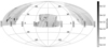 |
Fig. 1. Aitoff projection of the sensitivity of RASS data within BOSS footprint. Nominal sensitivity in the 0.5–2 keV band toward 4 counts is plotted. The units are ergs s−1 cm−2. The grid shows Equinox J2000.0 Equatorial coordinates. |
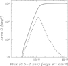 |
Fig. 2. Cumulative (Ω(> S), solid curve) and differential ( |

2.2. Source identification
We run the redMaPPer version 5.2 (Rykoff et al. 2014) on the position of every source (24 788 sources in the BOSS footprint), identifying the red sequence of maximum richness between redshifts 0.05 and 0.8. We search for the best optical center within 400 kpc from the X-ray center. We report the cluster richness both at X-ray and the optical positions, required corrections for the masked area of SDSS and photometric depths, which affect the error calculation for the richness. We calculate the probability of the center to be correct (Rykoff et al. 2014), which is useful for the weak-lensing modeling (e.g., Cibirka et al. 2017). We fold the BOSS area mask into the selection of CODEX. The catalog of cluster member galaxies has been released as a target catalog of SPIDERS (Clerc et al. 2016) and can be found online3.
We completed the spectroscopic follow-up campaign of CODEX clusters down to a richness of 10 through a number of programs on SDSS-II, III and IV and with the Nordic Optical Telescope. The first results are presented in Clerc et al. (2016, 2020) and Kirkpatrick et al. (in prep.) and these include a full characterization of the uncertainty in the photometric redshift estimate. We report on the 100% success rate in identification of clusters at z < 0.3, which required five spectroscopic members to achieve. At higher redshift the depths of the follow-up drive the identification success and this success reaches 100% once we are able to target > 7 member galaxies. The same galaxies form the bulk of the estimate of the cluster richness. Figure 3 shows the photometric depth correction factor used in calculating the reported SDSS cluster richness, ζ, which has an exponential increase toward high-z. This is a ratio of the richness of the cluster to the observed part. High values of ζ imply that only the tip of the cluster galaxy luminosity function is observed. ζ also describes the selection of the spectroscopically confirmed subsample, which is a combination of the threshold for spectroscopic cluster confirmation and the success rate of cluster member targeting. As the robustness of photometric identification relies on the actual number of galaxies used, to be consistent with other redMaPPer catalogs, we chose to use richness limit with redshift of at least ten member galaxies. While we also correct the richness for the masked area, the fraction of clusters with masking correction exceeding 20% is 3% of the sample and therefore does not require additional modeling, apart from the tests performed for galaxy cluster clustering (Lindholm et al., in prep.).
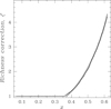 |
Fig. 3. Multiplicative richness correction due to photometric depths of the SDSS survey. The black histogram shows the actual correction applied and the gray curve shows our approximation of it as ζ = e5.5(z − 0.35) − 0.12 at z > 0.37. |
The resulting redshift range of CODEX clusters is 0.05–0.65. Performance of the redMaPPer has not been calibrated below a redshift of 0.1, and a systematic offset between the photometric and spectroscopic redshifts is found (Clerc et al. 2016). Large projection effects and the large size of X-ray sources also require additional care. We therefore do not discuss the properties of the z < 0.1 part of the catalog. A comparison of literature redshifts and redMaPPer measurements is also discussed in Rozo et al. (2015).
Using positions of random sources, we estimated a probability of the chance identification of a richness 20 source to be 10% in each 0.1 width bin of redshift in the range 0.1 < z < 0.6. In Fig. 4 we compare the completeness limits of the RASS and SDSS surveys toward the detection of a galaxy cluster. We use the scaling relation of Capasso et al. (2019) to express the survey mass limits in terms of (true) richness. Identification of RASS sources using the DES survey is considered in Klein et al. (2019). While this survey covers a different area, the strategy for source identification is similar. The 10% sensitivity curve of the CODEX survey matches well the definition of low (5%) contamination subsample in Klein et al. (2019), which we verify using an overlap area of two surveys, located in the Stripe 82 (Capasso et al. 2020). In order to reduce the effect of contamination down to 5%, we need to remove the sources with richness below the curve, and propagate this selection into the modeling. The analytical form of the selection reads
 (1)
(1)
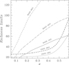 |
Fig. 4. Richness limits of the survey. The black curves show the 90% (dashed) and 50% (dotted) completeness limits PSDSS of redMaPPer cluster confirmation via SDSS data (Rykoff et al. 2014). The gray curves indicate the 10% (solid), 50% (long-dashed) and 90% (short-dashed) completeness limits of the RASS. The 10% curve also serves as a limit for low (5%, Klein et al. 2019) contamination subsample and is adopted as our selection PRASS. |
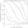 |
Fig. 5. Probability of cluster detection as a function of its core radius P(I|rc, ηob, β(μ)). The solid, dotted, dashed, long-dashed, dashed-dotted, long-dashed-dotted curves denote the calculation for ηob of 4, 5, 6, 8, 10, 15 counts, respectively. The range of core radii shown represent the cluster sample at a redshift of 0.25. |
In addition to X-ray completeness, in Fig. 4 we consider the effect of optical completeness and find it to be important for the modeling of CODEX both at z < 0.2 and z > 0.5. We use the following analytical function of the 50% optical completeness (λ denotes a natural logarithm of richness to simplify the notation for the log-normal distribution):
 (2)
(2)
which is obtained using the tabulations of Rykoff et al. (2014). We use an error function with the mean of λ50%(z) and a σ = 0.2, which reproduces the 75% and 90% quantiles of the distribution tabulated in Rykoff et al. (2014). We use the probability of the optical detection of the cluster in SDSS data as
 (3)
(3)
which is discussed further in Sect. 3.
2.3. CODEX catalog
Once an X-ray source has an optical counterpart, we can assign a redshift to it. This allows us to compute the source rest-frame properties such as luminosity. We apply the procedure of Finoguenov et al. (2007) to iteratively restore the X-ray luminosity. We obtain an initial guess on cluster mass, using M − LX relation and compute the missing source flux correction (A), taking into account the flux extraction aperture and the expected surface brightness profile of the source, given the mass (Käfer et al. 2019). In performing mass and temperature estimates, we use the XXL M − T (Lieu et al. 2016) and LX − T (Giles et al. 2016) relations, which is also consistent with CODEX weak-lensing calibration of Kettula et al. (2015). For small apertures, we use the PSF correction. Applying these corrections we obtain a new estimate of luminosity. We iterate this procedure 100 times. The resulting catalog of cluster properties is presented in Table 14. Column (1) lists CODEX source ID, (2) frequently used SPIDERS ID, Cols. (3–4) provides the coordinates of the X-ray center (FK5), Col. (5) provides the redMaPPer redshift, Cols. (6–7) provides the richness estimate and its error, Cols. (8–9) provide the coordinates of the best optical center (FK5), and Col. (10) gives the probability of this center to be correct. Columns (11–12) list the X-ray luminosity in the rest-frame 0.1–2.4 keV and its error, Col. (13) lists the temperature used in estimating the K-correction, Cols. (14–16) list A, K PSF corrections, Col. (17) lists the correction used in the computation of the optical richness, Cols. (18–19) the aperture-corrected flux of the source in the 0.5–2 keV band and its error, and Col. (20) lists the source flag (0 – clean catalog using Eq. (1), 1 – full catalog).
Calculation of LX at low statistics produces on average higher values of LX, compared to the true values due to asymmetrical shape of the Poisson distribution. The correction for the bias depends on the mass function of clusters and thus cosmology, in addition to the statistics of cluster detection. In Sect. 5 we reproduce the resulting LX distribution, while in Table 1 we present uncorrected properties.
Further insights into the LX computation are available using the spectroscopic identification of the sample and the final results of the SDSS program are presented in Clerc et al. (2020) and Kirkpatrick et al. (in prep.).
The clusters with richness greater than 60 in the previously poorly studied redshift range of 0.4 < z < 0.6 have been a subject of an CFHT follow-up (e.g., Cibirka et al. 2017; Kiiveri et al. 2020). The SPIDERS program has enabled a dynamical mass calibration of the sample (Capasso et al. 2019) in the full range of richness and redshifts. Stacked weak-lensing analysis of DECaLS data on z < 0.2 CODEX clusters confirmed the results of dynamical modeling (Phriksee et al. 2020). The results of these calibrations allow us to refine the modeling presented in this paper and evaluate the effect of calibration on the precision of cosmological parameters.
3. Modeling of X-ray cluster detection
We modeled the source detection as a probability given the number of detected source counts (ηob) and the shape parameters of the surface brightness (SB) distribution of the source P(I|ηob, SB), where I denotes the selection.
We measured the background level in the 0.5–2 keV RASS images, using source-free zones. Typically, the background level corresponds to a level of 1 background count in the smallest zone of detection with up to 16 background counts in the largest scales of detection. In the model we assume a dominant contribution of cosmic X-ray background to the background counts and use the exposure maps as a model for its spatial distribution. We note that strong flares in RASS data release 3 were filtered out by removing the corresponding time intervals.
We simulated the cluster detection as a function of total number of detected cluster counts, performing a simulation of each value of the cluster shape parameter grid 1000 times and trying 1000 realizations of the background for each simulated cluster image. The grid of the cluster shape parameters samples the parameters of the β-profile of clusters with surface brightness distributed with radius r as
 (4)
(4)
normalized to the total count, ηtrue, and sampling the distribution of core radii for clusters of given T, derived using a fixed β − T relation (Käfer et al. 2019). We sampled a cluster mass range between 13.5 and 15.3 in log10(M200c) to predict the shape of the cluster X-ray surface brightness (β, Rc) and a redshift range 0.1–0.6. We performed a Poisson realization of the simulated image and stored the results based on observed count rate (ηob) from 3 to 30. As we use multivariate log-normal distributions throughout this paper, we conveniently define the quantities rc ≡ ln(Rc), l ≡ ln(Lx), μ ≡ ln(M200c), λ ≡ ln(Richness). We denote the obtained grid as a probability of detection given the detected counts of the source (ηob), and shape parameters β and rc: P(I|ηob, β, rc). To use the results of Käfer et al. (2019), we substituted T with μ using M − T relation of Kettula et al. (2015).
As has been pointed out by Käfer et al. (2019), the cluster shape is covariant with the scatter in M − LX relation and we use their tabulations of the multivariate Gaussian distribution, P(rc, l|μ). While Käfer et al. (2019) characterize the cluster population at z < 0.1, the importance of the considered effects is reduced at z > 0.3, where all our clusters are nearly point-like for RASS; we deem this data sufficient. The effect of the covariant change in the core radius results in an even larger detectability of the cool core clusters. Not only do they have larger LX for a given mass, their peaked shape has a better chance of being detected (Eckert et al. 2011).
In addition to the covariance of X-ray luminosity and shape, we include a covariance of X-ray luminosity and richness based on the results of Farahi et al. (2019), leading to
![Mathematical equation: $$ \begin{aligned} P(l^\mathrm{true},r_c,\lambda | \mu ,z) = \frac{1}{ (2 \pi )^{3/2} | \boldsymbol{\Sigma } |^{1/2}} \exp \left[ - \frac{1}{2} \mathbf{X}^T \boldsymbol{\Sigma }^{-1} \mathbf{X}\right],\end{aligned} $$](/articles/aa/full_html/2020/06/aa37283-19/aa37283-19-eq6.gif) (5)
(5)
where the vector
 (6)
(6)
is defined using the scaling relations of Käfer et al. (2019), Mulroy et al. (2019) and Capasso et al. (2019). The covariance matrix Σ reads
 (7)
(7)
In this work we adopt the following values ρrcl|μ = −0.3, σrc|μ = 0.36 (Käfer et al. 2019), σλ|μ = 0.2 (Capasso et al. 2019; Mulroy et al. 2019), ρlλ|μ = −0.3 (Farahi et al. 2019), σl|μ = 0.46(1 − 0.61z) (Mantz et al. 2016); no measurement of ρrcλ|μ is published and thus this value is set to 0 in our work.
The effect of richness on the selection is only by offsetting the distributions of l and rc, and so for the purpose of determining the mass-richness relation, it is convenient to store just the effect of covariance on the selection function, replacing richness with  , storing P(I|μ, z, ν) and transforming P(rc, l, λ|μ, z) to P(rc, l|μ, ν, z)P(λ|μ, z), where only P(λ|μ, z) is varied in the scaling relation work (external to this paper). Given the freedom in treatment of the covariance ρrcλ|μ, we set it to zero, which makes Σ a block diagonal matrix, with two 2 × 2 elements (also explained as P(rc, l|μ, ν, z) = P(rc|μ, l, z)P(l|μ, ν, z)): Σl, λ and Σl,rc, whose inversion is analytical, resulting in
 (8)
(8)
The usefulness of this formula is a demonstration that covariance results in the offset of the distribution (for a graphical illustration of the offset, see also Capasso et al. 2019). Denoting the survey area Ω (deg2) and sensitivity S (ergs s−1 cm−2), which includes the effects of exposure and nH, we define the survey selection function as
 (9)
(9)
where
 (10)
(10)
The conversion of luminosity to counts uses the luminosity distance to the object dL(z), sensitivity S (counts per flux in ergs cm−2 s−1) and K-correction  , and
, and
 (11)
(11)
Figure 6 illustrates the resulting calculation for two values of ν: i) ν = 0, that is, clusters following the scaling relation ⟨λ|μ⟩ and ii) ν = 1.5, that is, clusters deviating by +1.5σλ|μ from the mean relation. This demonstrates the reduced sensitivity of the survey toward clusters deviating in richness. This matrix is used to fit the richness-mass relation (Kiiveri et al. 2020) and to constrain cosmology using the richness function (Ider Chitham et al. 2020).
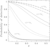 |
Fig. 6. Probability of cluster detection as a function of redshift. The solid, dotted, dashed, and long-dashed curves denote the calculation for log10(M200c/M⊙) of 14, 14.5, 14.8, and 15, respectively. The gray curves show the same calculation for clusters with richness deviating from the mass-richness relation by +1.5σλ|μ. |
The modeling of the sample takes a mass function of clusters (for a discussion of our choice of cluster mass functions, see Ider Chitham et al. 2020); predicts a covariant distribution of LX and richness for each mass value; associates the shape parameters of the cluster with distribution of LX; performs a calculation of the probability of cluster detection in each element of effective exposure; and finally obtains a corresponding effective area, which is added to the total area. In the above equations, λ corresponds to the true parameter, so only the intrinsic scatter in the μ − λ relation is taken into account, which for CODEX has been measured to be 0.2 (Capasso et al. 2019; Mulroy et al. 2019). In generating the SDSS richness, we need to account for the depth of the SDSS survey, using the scale value ζ (see Fig. 3 for its redshift evolution), as discussed in Capasso et al. (2019). This extra scatter is not covariant with X-ray properties, so we use  , where we are accounting for an additional detail that the scatter in the observed richness is a function of true richness and not the mean true richness. We also report the measurement errors on richness, which include the effect of masking and uncertainty of local background subtraction. A comparison with deeper data reveals that accounting for both error terms is important.
The expected number of clusters within a given photon count,  , and redshift, Δzj, bin is written as
 (12)
(12)
where ΔΩ is the geometric survey area in steradians and (dV/dzdΩ) is the comoving volume element, and we use Hogg (1999) calculation for the flat Universe. The halo number density as a function of the observed photon counts ηob – (dn(ηob, S, z))/(dηob) – can be related to the theoretical halo mass function, n(μ, z), through
 (13)
(13)
where
 (14)
(14)
corresponds to a probability of the observed richness to exceed the selection threshold needed to clean the RASS data (Eq. (1)), which is a complementary error function (erfc). We also add an account for the optical cluster selection completeness of SDSS PSDSS(I|λ, z), which is discussed above (Eq. (3)).
Comparing the measurements requires an additional detail, since there we apply the aperture and PSF corrections. When we simulated the detection, we used the full count produced by a simulated cluster, ηob. We calibrated our flux restoration routine on simulations, determining the probability of reporting ηmeas, given an input ηob and the background realizations (ηbkg(ra)ob − ⟨ηbkg(ra)ob⟩), conditioned to source detection. We used Poisson probability for calculating  . We estimated
  using source-free zones in each RASS field. The function obtained this way (i.e., P(ηmeas|ηob, z, S)) absorbs the probability of detecting a certain extent of the source P(ra|rc, ηob, β(μ)) and its effect on the performed extrapolation of the flux:
 (15)
(15)
where ηmeas is the modeled corrected count, to be compared to that reported in the CODEX catalog; ra is the flux extraction aperture in simulations and ηa– background-corrected aperture simulated count; R500 is the radius effectively encompassing X-ray emission (e.g., Finoguenov et al. 2007, and since it is not known a priori, it requires iterations), and is therefore effectively a function R500(ηob, ra, z, S). The quantity A is the resulting aperture correction. To compute R500 we used the concentration-mass relation of Dutton & Macciò (2014) to estimate R500 from M200(LX).
The ra-dependent corrections are close to unity, with typical values in the 1 − 1.20 range. High aperture corrections, exceeding 1.5 imply that flux of the emission is much larger than its extent. These are cases of nearby sources, but are also a result of flux contamination. For low-z (z < 0.15) sources, where the aperture corrections are large, we are able to re-extract the counts using an aperture covering R500, thus removing the need for a corrections and verify an absence of any bias in the flux estimate. So, finally,
 (16)
(16)
It is clear that changes in the sensitivity of the survey result in the mixing of various contributions to the count distribution. It is therefore more convenient to reconstruct the observed LX distribution as follows:
 (17)
(17)
Practical implementation of Eq. (16) uses a low and high statistics approximations with a switch at 20 detected counts. For low statistics, we find ηa ≈ ηob with a much lower scatter, compared to an attempt to reproduce ηmeas. Thus, in modeling the counts, performed in Fig. 10, we mix aperture (dominant in high-z XLF and lowest LX low-z bin) and full X-ray luminosities from the data and do the same in the modeling.
4. Modeling of the association between X-ray source and optical cluster
We consider the following processes to result in the association between an X-ray source and the optical cluster:
1. Chance association between an X-ray source and an optical cluster.
2. Detection of the optical cluster due to AGN activity of its member galaxies.
3. Detection of the optical cluster due to thermal emission of the ICM
We calculated the probability of a chance identification by placing random points on the sky and running the redMaPPer algorithm on these random points. We obtained the probability of chance identification as a function of redshift for two cuts in detected optical richness, 10 and 20. While within a factor of 1.5, there are no changes in the chance identification rate with redshift, there is a strong increase in the chance identification toward low values of richness, going from 10% for richness of 20 to 30% for richness of 10.
The probability of the identification of a cluster predominantly through its AGN activity is driven by the probability of a cluster to host an AGN, which is given by the AGN halo occupation distribution (HOD), and a probability of AGN to have a certain luminosity, which is given by the AGN XLF. We used the HOD results of Allevato et al. (2012) and the Ebrero et al. (2009) luminosity function for 0.5–2 keV to perform the calculation. The typical luminosity of AGN, calculated using the AGN XLF, is 1044 ergs s−1, where the probability of finding such an AGN in a cluster is 0.05 × (1 + z)3.3. There is no dependence on halo mass at M200c > 1013 M⊙ predicted by the model. This modeling allows us to conclude that AGNs only provide a modest contamination-to-cluster luminosity, which is important only at lower redshifts, where our sensitivity is below the typical AGN luminosity. According to this modeling, the main contribution to cluster counts are AGNs detected in galaxy groups. High X-ray luminosity and low optical richness systems are therefore regarded as AGNs in groups or chance identification.
In Fig. 7 we compare the measured cluster richness function with the prediction based on ΛCDM and our AGN contamination model. The AGN luminosity produces an additional component, which at zero order is simply a fraction of all clusters of a given richness that we have not yet detected. The evolution of the fraction of the detected clusters as a function of redshift is due to two competing effects: the evolution of the AGN XLF and the evolution of the threshold luminosity of AGN, which leads to a decreased AGN detectivity per cluster.
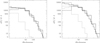 |
Fig. 7. Richness function of CODEX clusters in the 0.1 < z < 0.3 (left panel) and 0.1 < z < 0.6 range (right panel). The solid gray histogram shows the data; the dotted histogram shows the contribution to the total counts from the clusters detected through their AGN activity; the dashed histogram shows the contribution from clusters detected through their thermal emission; and the solid histogram shows the total expected number of detection, which provides a good match to the data. The dotted gray histogram shows the data with excision of points deviating beyond the 2σ from the richness−LX relation. |
In addition to detection of new systems, AGNs can contribute to the total luminosity of the clusters, which are selected primarily by the ICM luminosity. This contribution is discussed in Clerc et al. (2016) and is below the 10% level.
We now compare these results with the contamination calculation of Klein et al. (2019). As we mentioned the contaminated zone outlined in Klein et al. (2019) corresponds to the 10% X-ray completeness curve in our calculation. There, truly detected clusters are 10%, while the rest 90% can be identified by chance (richness-dependent process) or by AGN activity (nearly richness independent). As we mentioned, the AGN activity yields 2% identification and the chance identification is at most 10% for richness of 20. The fractional importance of the contamination is therefore 50% of the total at the lowest value of richness considered in this work and drops to 9% at high redshift, where it is dominated by AGN HOD, while chance identifications are rare as number of clusters of high richness is low. This consideration allows us to conclude that contamination is indeed driven by the lack of real detections.
In Fig. 8 we compare the richness distributions of CODEX clusters, its subsamples, based on flux and redshift, and the literature sample MCXC (Piffaretti et al. 2011) matched to CODEX clusters in order to obtain a richness estimate. The literature sample is primarily composed of the bright X-ray clusters and its distribution does not significantly change by imposing a cut on the flux of 10−12 ergs cm−2 s−1. We imposed a similar flux cut to the CODEX sample to illustrate the effect of a different flux. We also tested a redshift cut of z < 0.3 on the CODEX sample to eliminate the effect of the noise in the optical data. The comparison points out that the literature sample of clusters systematically lacks identification of clusters of richness below 70 (obtained by restricting the comparison to both low-z and high-flux subsamples), which corresponds to the clusters at the limit of the Abell cluster definition. Some of the literature (e.g., Böhringer et al. 2002) removal of sources based on the identification with an optical QSO, which can partially account for the difference. Also, the NORAS survey that entered MCXC was not complete (Böhringer et al. 2017).
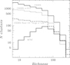 |
Fig. 8. Richness distribution of CODEX clusters (solid black histogram) compared to a subsample of CODEX clusters with flux above 10−12 ergs cm−2 s−1 (dashed black histogram), z < 0.3 CODEX clusters (dotted black histogram), and the matched MCXC clusters (solid gray histogram). The comparison shows a deficiency in the low richness identifications present in the MCXC catalog. |
In the parallel effort of Comparat et al. (2020), RASS sources are identified using NWAY (Salvato et al. 2018). Using the overlap of CODEX catalog with the DR16 area, we verified our estimates of contamination based on the alternative matches provided by NWAY. Using the 1281 clusters in the overlap clean catalog, we find 78 sources identified as AGN, 4 as BL LAC, and 3 as stars; 22 of these sources have matching redshifts to CODEX clusters within the redMaPPer errors. This corresponds to a 4.9% chance association and a 1.7% chance of flux contamination. Similarly, for a total sample of 6240 CODEX clusters in the DR16 area, 975 (263 matching in redshift) are identified as AGN, 26 (6 matching in redshift) as BL LACs, and 26 as stars. This corresponds to a 12.1% chance association and a 4.3% chance of flux contamination for the full sample. These numbers correspond well to our estimates of catalog purity and illustrate the effectiveness of our catalog cleaning method. In Clerc et al. (2020) we estimate the effect of AGN contamination on high-z XLF as 15%, while this effect is about 2% for the low-z XLF. In the modeling, we corrected the high-z XLF for this and add 5% fractional errors to account for uncertainty of the correction. We attribute the increased importance of AGN in high-z part of the sample to the increased scatter in SDSS richness estimate, which reduces the efficiency of cleaning the sample at high-z. For improvements using deeper photometry, see Ider Chitham et al. (2020).
5. Evolution of cluster X-ray luminosity function
One of the direct measurements that CODEX provides is the evolution of the XLF of galaxy clusters. The evolution of XLF combines a decrease in the number of clusters of given mass with higher X-ray luminosity per given mass at higher redshifts. While, we are using red sequence redshifts in calculation of the X-ray luminosity, we verified that use of spectroscopic redshift does not change the XLF (Clerc et al. 2020) and so we can omit the integration over the redshift uncertainties.
In Fig. 9 we present CODEX constraints on the evolution of the cluster XLF measured in the redshift interval 0.1 < z < 0.6 using bins of redshift of 0.1. We only show the data without strong (exceeding a factor of 2) completeness correction, as those are sensitive to the adopted scaling relations as well as the impact of the assumed distance-redshift relation on detection statistics. The completeness correction is calculated by rationing the predicted distribution of clusters on luminosity accounting for the sample properties (described above in Eqs. (13)–(17)) and that assuming no selection effects and infinite statistics as follows:
 (18)
(18)
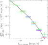 |
Fig. 9. X-ray luminosity function of CODEX clusters in the redshift range 0.1–0.6 (0.1–0.2 green, 0.2–0.3 red, 0.3–0.4 blue, 0.4–0.5 magenta, 0.5–0.6 cyan). At low LX we also show the COSMOS XLF, for comparison as green dotted crosses. The solid black curve shows a Schechter function description of REFLEX XLF (Böhringer et al. 2002). Our results agree well with the REFLEX and reveal no strong redshift evolution of XLF. |
The main results seen in Fig. 9 are in agreement with the XLF determined from other low-z (z < 0.3) studies, and a lack of strong evolution of the XLF with redshift.
In order to compare the observed luminosity function with the expectations of different cosmological models, we need to adopt a mass calibration. At the moment, the 0.3 < z < 0.6 part of the CODEX scaling relations are not yet tightly constrained, while the available studies extending to a redshift of one argue in favor of the self-similar scaling for these relations outside of the cool core (McDonald et al. 2019). Therefore, in this work we consider whether the observed lack of evolution of XLF can be explained by a combination of self-similar evolution of scaling relations and a change in some basic cosmological parameters, limiting the study to ΩM and σ8. The dominant systematics of this assumption is a lack of constraints on the evolution of the cool core and AGN contamination in the CODEX high-z sample. These need to be understood better by future work. Adjusting the mass calibration for changing the ΩM is not required in the scaling relations based on dynamical mass estimates done with respect to the critical density, as  ; the assumption of geometry of the Universe in calculating LX is canceled out by the calibration procedure, which establishes the link to the mass and so does not need to be updated on average. The mass is both measured and used in defining the mass function with the same scaling for the Hubble constant. However, since our modeling of the high-z sample considers a self-similar evolution of scaling relations instead of direct determination, we need to allow for an effect of geometry of the Universe on LX.
In Fig. 10 we compare the observed number of clusters with the results of the modeling presented in this paper. In Fig. 11, we present the associated cosmological parameters. We use two redshift bins to simplify the presentation of the results: low redshift bin 0.1 < z < 0.3 and high redshift bin, 0.3 < z < 0.6. We estimate the errors (σij) based on the measured number of clusters. Given the large area of the survey and the high redshift bins used, we can ignore the sample variance term in the mass-function calculation. In Fig. 10 we plot the models that satisfy both high-z and low-z sample.
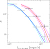 |
Fig. 10. Number of CODEX clusters in the redshift range 0.1–0.3 (gray) and 0.3–0.6 (black), compared to the allowed range of ΛCDM cosmological parameters. Low-z solutions are shown in blue (best fit) and cyan (extremes of 95% confidence interval), high-z – in red (best fit) and magenta (extremes of 95% confidence interval). The numbers are corrected for the expected AGN contamination and luminosity is a mix of corrected and uncorrected values for high and low statistics subsample. |
Lower values of ΩM predict a slower evolution of the mass function and a larger volume, which is partially compensated by the slower evolution of the scaling relation, and smaller cluster X-ray detected count rates, which would be converted into smaller LX under a fixed cosmology. The normalization of the XLF can be adjusted by changing σ8, but it is constrained by the slope of the XLF, which in our case is measured accurately only at low-z.
In calculating the best fit, we used a grid of models, covering values of Ωm in the (0.1 − 0.4) interval and the values of σ8 in the (0.7 − 1.0) interval. We computed the likelihood of the solution using χ2. The minimum of the
 (19)
(19)
is comparable with the number of degrees of freedom and thus the solutions are statistically acceptable. To compute the error intervals on cosmological parameters, we used the deviations from the minimum. We quote the errors associated with two parameters of interest, so 1σ corresponds to a Δχ2 = 2.3.
The cosmology of low-z sample is comparable with previous similar studies (Böhringer et al. 2014); slight differences in the best-fit values are primarily due to the adopted mass calibration, which is well within the reported associated uncertainties. Thus, our revision in the cluster identification did not result in the change of the cosmological constraints coming from low-z RASS surveys, with a possible exception of the work of Mantz et al. (2016), where we disagree on the adopted M − LX relation. Our relation has a 10% lower normalization in mass, coming from LoCuSS and CCCP studies (for a careful discussion of the problem, see Smith et al. 2016), and confirmed by the CODEX mass calibration efforts (Capasso et al. 2020; Phriksee et al. 2020). We deem our low-z calibration to be good to 5% in mass, which results in the associated systematical uncertainty in Ωm of 0.015. For the discussion of comparison of low and high-z XLF, this uncertainty would shift the final solution, but does not result in a larger overlap in the solutions; therefore we do not show this uncertainty in Fig. 11. The main result, seen in Fig. 11 consists in finding that after correction for the flux reconstruction at low statistics and AGN contamination, the cosmological constraints coming from the high-z CODEX cluster sample largely overlap with those of low redshift, leading to a large allowed range of cosmological parameters. Within a flat ΛCDM and an assumption of self-similar evolution of scaling relations, the required cosmological parameters are Ωm = 0.270 ± 0.06 ± 0.015(syst.) and σ8 = 0.79 ± 0.05 ± 0.015(syst.), quoting a 68% confidence interval, with a combined σ8(Ωm/0.3)0.3 = 0.77 ± 0.015 ± 0.015(syst.). Comparing our solution to the literature on galaxy clusters, our solution overlaps with the parameter space in overlap with all cluster surveys (Böhringer et al. 2014; Henry et al. 2009; Bocquet et al. 2019; Vikhlinin et al. 2009) and Fig. 11 can serve as a forecast for the importance of the calibration of scaling relation work at high-z.
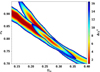 |
Fig. 11. Constraints on the flat ΛCDM model by the CODEX cluster XLF. The 0.1 < z < 0.3, drawn below all other shades (bottom right corner), and 0.3 < z < 0.6 (top right corner) constraints are shown along with their overlap (drawn on top of all the areas). The color shows the Δχ2 from the minimum with 2.3, 4.6, and 9.2 corresponding to 68, 90, and 99% confidence level for two parameters (Lampton et al. 1976). |
6. Conclusions
We present a new, large catalog of X-ray clusters detected in the SDSS area. The catalog is constructed with the aim of an efficient spectroscopic follow-up program of SDSS, which has completed data acquisition process in March 2019. This paper describes the catalog construction to accompany the final (DR16) data release.
Despite the low photon statistics of RASS, we show that we can convincingly model the survey selection function. We point out that low-richness clusters are under-represented in the identification process of X-ray clusters, and this needs to be included in the modeling of the sample selection. We provide the forward modeling of such a selection and apply it to the sample to construct the XLFs of the survey. Our main result consists in the lack of evolution of cluster XLF. However, low statistics associated with the flux measurement at high-z redshift and AGN contamination were found to be of large importance in understanding the effect, while the associated constraints on the cosmological parameters are consistent with those of other cluster surveys. As with most new cluster samples, more work on understanding the properties of clusters will serve toward improving the robustness of the results and uniqueness of CODEX consists in its largest calibration database on cluster dynamics, which has yet to be fully explored.
Unless explicitly noted otherwise, all observed values quoted throughout this paper are calculated by adopting a ΛCDM cosmological model, where H0 = 70 km s−1 Mpc−1, ΩM = 0.3, ΩΛ = 0.7. We quote X-ray flux in the observer’s 0.5–2.0 keV band and rest-frame luminosity in the 0.1–2.4 keV band and provide confidence intervals on the 68% level. FK5 Epoch J2000.0 coordinates are used throughout.
The table is available at the CDS. Spectroscopic properties of CODEX clusters are released as a part of SDSS-IV DR16 under SPIDERS cluster catalog.
Acknowledgments
We thank the referee for their comments which improved the quality of this paper. Funding for the Sloan Digital Sky Survey IV has been provided by the Alfred P. Sloan Foundation, the US Department of Energy Office of Science, and the Participating Institutions. SDSS-IV acknowledges support and resources from the Center for High-Performance Computing at the University of Utah. The SDSS web site is www.sdss.org. SDSS-IV is managed by the Astrophysical Research Consortium for the Participating Institutions of the SDSS Collaboration including the Brazilian Participation Group, the Carnegie Institution for Science, Carnegie Mellon University, the Chilean Participation Group, the French Participation Group, Harvard-Smithsonian Center for Astrophysics, Instituto de Astrofísica de Canarias, The Johns Hopkins University, Kavli Institute for the Physics and Mathematics of the Universe (IPMU)/University of Tokyo, the Korean Participation Group, Lawrence Berkeley National Laboratory, Leibniz Institut für Astrophysik Potsdam (AIP), Max-Planck-Institut für Astronomie (MPIA Heidelberg), Max-Planck-Institut für Astrophysik (MPA Garching), Max-Planck-Institut für Extraterrestrische Physik (MPE), National Astronomical Observatories of China, New Mexico State University, New York University, University of Notre Dame, Observatário Nacional/MCTI, The Ohio State University, Pennsylvania State University, Shanghai Astronomical Observatory, United Kingdom Participation Group, Universidad Nacional Autónoma de México, University of Arizona, University of Colorado Boulder, University of Oxford, University of Portsmouth, University of Utah, University of Virginia, University of Washington, University of Wisconsin, Vanderbilt University, and Yale University. Based on observations made with the Nordic Optical Telescope, operated by the Nordic Optical Telescope Scientific Association at the Observatorio del Roque de los Muchachos, La Palma, Spain, of the Instituto de Astrofisica de Canarias.
References
- Ahumada, R., Allende Prieto, C., Almeida, A., et al. 2019, ArXiv e-prints [arXiv:1912.02905] [Google Scholar]
- Allevato, V., Finoguenov, A., Hasinger, G., et al. 2012, ApJ, 758, 47 [NASA ADS] [CrossRef] [Google Scholar]
- Bocquet, S., Dietrich, J. P., Schrabback, T., et al. 2019, ApJ, 878, 55 [NASA ADS] [CrossRef] [Google Scholar]
- Böhringer, H., Collins, C. A., Guzzo, L., et al. 2002, ApJ, 566, 93 [NASA ADS] [CrossRef] [Google Scholar]
- Böhringer, H., Schuecker, P., Guzzo, L., et al. 2004, A&A, 425, 367 [NASA ADS] [CrossRef] [EDP Sciences] [Google Scholar]
- Böhringer, H., Chon, G., Collins, C. A., et al. 2013, A&A, 555, A30 [NASA ADS] [CrossRef] [EDP Sciences] [Google Scholar]
- Böhringer, H., Chon, G., & Collins, C. A. 2014, A&A, 570, A31 [NASA ADS] [CrossRef] [EDP Sciences] [Google Scholar]
- Böhringer, H., Chon, G., Retzlaff, J., et al. 2017, AJ, 153, 220 [NASA ADS] [CrossRef] [Google Scholar]
- Boese, F. G. 2000, A&AS, 141, 507 [NASA ADS] [CrossRef] [EDP Sciences] [Google Scholar]
- Boller, T. 2017, Astron. Nachr., 338, 972 [CrossRef] [Google Scholar]
- Blanton, M. R., Bershady, M. A., Abolfathi, B., et al. 2017, AJ, 154, 28 [NASA ADS] [CrossRef] [Google Scholar]
- Bulbul, E., Chiu, I.-N., Mohr, J. J., et al. 2019, ApJ, 871, 50 [NASA ADS] [CrossRef] [Google Scholar]
- Capasso, R., Mohr, J. J., Saro, A., et al. 2019, MNRAS, 486, 1594 [CrossRef] [Google Scholar]
- Capasso, R., Mohr, J. J., Saro, A., et al. 2020, MNRAS, 494, 2736 [CrossRef] [Google Scholar]
- Cibirka, N., Cypriano, E. S., Brimioulle, F., et al. 2017, MNRAS, 468, 1092 [NASA ADS] [CrossRef] [Google Scholar]
- Clerc, N., Merloni, A., Zhang, Y.-Y., et al. 2016, MNRAS, 463, 4490 [NASA ADS] [CrossRef] [Google Scholar]
- Clerc, N., Kirkpatrick, C., Finoguenov, A., et al. 2020, MNRAS, submitted [Google Scholar]
- Comparat, J., Merloni, A., Dwelly, T., et al. 2020, A&A, 636, A97 [NASA ADS] [CrossRef] [EDP Sciences] [Google Scholar]
- Dawson, K. S., Schlegel, D. J., Ahn, C. P., et al. 2013, AJ, 145, 10 [Google Scholar]
- Dawson, K. S., Kneib, J.-P., Percival, W. J., et al. 2016, AJ, 151, 44 [NASA ADS] [CrossRef] [Google Scholar]
- Dutton, A. A., & Macciò, A. V. 2014, MNRAS, 441, 3359 [NASA ADS] [CrossRef] [Google Scholar]
- Ebrero, J., Carrera, F. J., Page, M. J., et al. 2009, A&A, 493, 55 [NASA ADS] [CrossRef] [EDP Sciences] [Google Scholar]
- Eckert, D., Molendi, S., & Paltani, S. 2011, A&A, 526, A79 [NASA ADS] [CrossRef] [EDP Sciences] [Google Scholar]
- Farahi, A., Mulroy, S. L., Evrard, A. E., et al. 2019, Nat. Commun., 10, 2504 [NASA ADS] [CrossRef] [Google Scholar]
- Finoguenov, A., Guzzo, L., Hasinger, G., et al. 2007, ApJS, 172, 182 [NASA ADS] [CrossRef] [Google Scholar]
- Giles, P. A., Maughan, B. J., Pacaud, F., et al. 2016, A&A, 592, A3 [NASA ADS] [CrossRef] [EDP Sciences] [Google Scholar]
- Hasinger, G. 1996, A&AS, 120, 607 [Google Scholar]
- Henry, J. P., Evrard, A. E., Hoekstra, H., et al. 2009, ApJ, 691, 1307 [NASA ADS] [CrossRef] [Google Scholar]
- Hogg, D. W. 1999, ArXiv e-prints [arXiv:astro-ph/9905116] [Google Scholar]
- Ider Chitham, J., Comparat, J., Finoguenov, A., et al. 2020, MNRAS, submitted [Google Scholar]
- Käfer, F., Finoguenov, A., Eckert, D., et al. 2019, A&A, 628, A43 [NASA ADS] [CrossRef] [EDP Sciences] [Google Scholar]
- Kalberla, P. M. W., Burton, W. B., Hartmann, D., et al. 2005, A&A, 440, 775 [NASA ADS] [CrossRef] [EDP Sciences] [Google Scholar]
- Kettula, K., Giodini, S., van Uitert, E., et al. 2015, MNRAS, 451, 1460 [NASA ADS] [CrossRef] [Google Scholar]
- Kiiveri, K., Gruen, D., Finoguenov, A., et al. 2020, MNRAS, submitted [Google Scholar]
- Klein, M., Grandis, S., Mohr, J. J., et al. 2019, MNRAS, 488, 739 [CrossRef] [Google Scholar]
- Lampton, M., Margon, B., & Bowyer, S. 1976, ApJ, 208, 177 [NASA ADS] [CrossRef] [Google Scholar]
- Lieu, M., Smith, G. P., Giles, P. A., et al. 2016, A&A, 592, A4 [NASA ADS] [CrossRef] [EDP Sciences] [Google Scholar]
- Mantz, A. B., Allen, S. W., Morris, R. G., et al. 2016, MNRAS, 463, 3582 [NASA ADS] [CrossRef] [Google Scholar]
- McDonald, M., Allen, S. W., Hlavacek-Larrondo, J., et al. 2019, ApJ, 870, 85 [CrossRef] [Google Scholar]
- Mirkazemi, M., Finoguenov, A., Pereira, M. J., et al. 2015, ApJ, 799, 60 [NASA ADS] [CrossRef] [Google Scholar]
- Mulroy, S. L., Farahi, A., Evrard, A. E., et al. 2019, MNRAS, 484, 60 [NASA ADS] [CrossRef] [Google Scholar]
- Oh, S., Mulchaey, J. S., Woo, J.-H., et al. 2014, ApJ, 790, 43 [NASA ADS] [CrossRef] [Google Scholar]
- Phriksee, A., Jullo, E., Limousin, M., et al. 2020, MNRAS, 491, 1643 [CrossRef] [Google Scholar]
- Piffaretti, R., Arnaud, M., Pratt, G. W., et al. 2011, A&A, 534, A109 [NASA ADS] [CrossRef] [EDP Sciences] [Google Scholar]
- Planck Collaboration XXIV. 2016, A&A, 594, A24 [NASA ADS] [CrossRef] [EDP Sciences] [Google Scholar]
- Planck Collaboration VI. 2020, A&A, in press https://doi.org/10.1051/0004-6361/201833910 [Google Scholar]
- Rozo, E., Rykoff, E. S., Becker, M., et al. 2015, MNRAS, 453, 38 [NASA ADS] [CrossRef] [Google Scholar]
- Rykoff, E. S., Rozo, E., Busha, M. T., et al. 2014, ApJ, 785, 104 [NASA ADS] [CrossRef] [Google Scholar]
- Salvato, M., Buchner, J., Budavári, T., et al. 2018, MNRAS, 473, 4937 [NASA ADS] [CrossRef] [Google Scholar]
- Smith, G. P., Mazzotta, P., Okabe, N., et al. 2016, MNRAS, 456, L74 [NASA ADS] [CrossRef] [Google Scholar]
- Truemper, J. 1993, Science, 260, 1769 [NASA ADS] [CrossRef] [PubMed] [Google Scholar]
- Vikhlinin, A., McNamara, B. R., Forman, W., et al. 1998, ApJ, 502, 558 [NASA ADS] [CrossRef] [Google Scholar]
- Vikhlinin, A., Kravtsov, A. V., Burenin, R. A., et al. 2009, ApJ, 692, 1060 [NASA ADS] [CrossRef] [Google Scholar]
- Voges, W., Aschenbach, B., Boller, T., et al. 1999, A&A, 349, 389 [NASA ADS] [Google Scholar]
- York, D. G., Adelman, J., Anderson, J. E., et al. 2000, AJ, 120, 1579 [CrossRef] [Google Scholar]
All Figures
|
Fig. 1. Aitoff projection of the sensitivity of RASS data within BOSS footprint. Nominal sensitivity in the 0.5–2 keV band toward 4 counts is plotted. The units are ergs s−1 cm−2. The grid shows Equinox J2000.0 Equatorial coordinates. |
| In the text | |
|
Fig. 2. Cumulative (Ω(> S), solid curve) and differential ( |
| In the text | |
|
Fig. 3. Multiplicative richness correction due to photometric depths of the SDSS survey. The black histogram shows the actual correction applied and the gray curve shows our approximation of it as ζ = e5.5(z − 0.35) − 0.12 at z > 0.37. |
| In the text | |
|
Fig. 4. Richness limits of the survey. The black curves show the 90% (dashed) and 50% (dotted) completeness limits PSDSS of redMaPPer cluster confirmation via SDSS data (Rykoff et al. 2014). The gray curves indicate the 10% (solid), 50% (long-dashed) and 90% (short-dashed) completeness limits of the RASS. The 10% curve also serves as a limit for low (5%, Klein et al. 2019) contamination subsample and is adopted as our selection PRASS. |
| In the text | |
|
Fig. 5. Probability of cluster detection as a function of its core radius P(I|rc, ηob, β(μ)). The solid, dotted, dashed, long-dashed, dashed-dotted, long-dashed-dotted curves denote the calculation for ηob of 4, 5, 6, 8, 10, 15 counts, respectively. The range of core radii shown represent the cluster sample at a redshift of 0.25. |
| In the text | |
|
Fig. 6. Probability of cluster detection as a function of redshift. The solid, dotted, dashed, and long-dashed curves denote the calculation for log10(M200c/M⊙) of 14, 14.5, 14.8, and 15, respectively. The gray curves show the same calculation for clusters with richness deviating from the mass-richness relation by +1.5σλ|μ. |
| In the text | |
|
Fig. 7. Richness function of CODEX clusters in the 0.1 < z < 0.3 (left panel) and 0.1 < z < 0.6 range (right panel). The solid gray histogram shows the data; the dotted histogram shows the contribution to the total counts from the clusters detected through their AGN activity; the dashed histogram shows the contribution from clusters detected through their thermal emission; and the solid histogram shows the total expected number of detection, which provides a good match to the data. The dotted gray histogram shows the data with excision of points deviating beyond the 2σ from the richness−LX relation. |
| In the text | |
|
Fig. 8. Richness distribution of CODEX clusters (solid black histogram) compared to a subsample of CODEX clusters with flux above 10−12 ergs cm−2 s−1 (dashed black histogram), z < 0.3 CODEX clusters (dotted black histogram), and the matched MCXC clusters (solid gray histogram). The comparison shows a deficiency in the low richness identifications present in the MCXC catalog. |
| In the text | |
|
Fig. 9. X-ray luminosity function of CODEX clusters in the redshift range 0.1–0.6 (0.1–0.2 green, 0.2–0.3 red, 0.3–0.4 blue, 0.4–0.5 magenta, 0.5–0.6 cyan). At low LX we also show the COSMOS XLF, for comparison as green dotted crosses. The solid black curve shows a Schechter function description of REFLEX XLF (Böhringer et al. 2002). Our results agree well with the REFLEX and reveal no strong redshift evolution of XLF. |
| In the text | |
|
Fig. 10. Number of CODEX clusters in the redshift range 0.1–0.3 (gray) and 0.3–0.6 (black), compared to the allowed range of ΛCDM cosmological parameters. Low-z solutions are shown in blue (best fit) and cyan (extremes of 95% confidence interval), high-z – in red (best fit) and magenta (extremes of 95% confidence interval). The numbers are corrected for the expected AGN contamination and luminosity is a mix of corrected and uncorrected values for high and low statistics subsample. |
| In the text | |
|
Fig. 11. Constraints on the flat ΛCDM model by the CODEX cluster XLF. The 0.1 < z < 0.3, drawn below all other shades (bottom right corner), and 0.3 < z < 0.6 (top right corner) constraints are shown along with their overlap (drawn on top of all the areas). The color shows the Δχ2 from the minimum with 2.3, 4.6, and 9.2 corresponding to 68, 90, and 99% confidence level for two parameters (Lampton et al. 1976). |
| In the text | |
Current usage metrics show cumulative count of Article Views (full-text article views including HTML views, PDF and ePub downloads, according to the available data) and Abstracts Views on Vision4Press platform.
Data correspond to usage on the plateform after 2015. The current usage metrics is available 48-96 hours after online publication and is updated daily on week days.
Initial download of the metrics may take a while.