| Issue |
A&A
Volume 637, May 2020
|
|
|---|---|---|
| Article Number | A93 | |
| Number of page(s) | 22 | |
| Section | Planets and planetary systems | |
| DOI | https://doi.org/10.1051/0004-6361/201937050 | |
| Published online | 27 May 2020 | |
The CARMENES search for exoplanets around M dwarfs
A super-Earth planet orbiting HD 79211 (GJ 338 B)★
1
Centro de Astrobiología (CSIC-INTA),
Carretera de Ajalvir km 4,
28850
Torrejón de Ardoz,
Madrid,
Spain
e-mail: This email address is being protected from spambots. You need JavaScript enabled to view it.
2
Instituto de Astrofísica de Canarias,
Av. Vía Láctea s/n,
38205
La Laguna,
Tenerife,
Spain
3
Departamento de Astrofísica, Universidad de La Laguna,
38206
La Laguna,
Tenerife,
Spain
4
Institut für Astrophysik, Georg-August-Universität,
Friedrich-Hund-Platz 1,
37077
Göttingen,
Germany
5
Instituto de Astrofísica de Andalucía (IAA-CSIC),
Glorieta de la Astronomía s/n,
18008
Granada,
Spain
6
Department of Physics, Ariel University,
Ariel
40700,
Israel
7
Departamento de Física de la Tierra y Astrofísica & UPARCOS-UCM (Ins. de Física de Partículas y del Cosmos de la UCM), Facultad de Ciencias Físicas, Universidad Complutense de Madrid,
28040
Madrid,
Spain
8
Institut de Ciències de l’Espai (ICE, CSIC),
Campus UAB, c/ de Can Magrans s/n,
08193
Bellaterra,
Barcelona,
Spain
9
Institut d’Estudis Espacials de Catalunya (IEEC),
08034
Barcelona,
Spain
10
Landessternwarte, Zentrum für Astronomie der Universtät Heidelberg,
Königstuhl 12,
69117
Heidelberg,
Germany
11
School of Physics and Astronomy, Queen Mary University of London,
327 Mile End Road,
London
E1 4NS,
UK
12
Centro Astronómico Hispano-Alemán (CSIC-MPG), Observatorio Astronómico de Calar Alto, Sierra de los Filabres,
04550
Gérgal,
Almería,
Spain
13
Thüringer Landessternwarte Tautenburg,
Sternwarte 5,
07778
Tautenburg,
Germany
14
Max-Planck-Institut für Astronomie,
Königstuhl 17,
69117
Heidelberg,
Germany
15
Hamburger Sternwarte,
Gojenbergsweg 112,
21029
Hamburg,
Germany
Received:
4
November
2019
Accepted:
6
March
2020
Abstract
Aims. We report on radial velocity time series for two M0.0 V stars, GJ 338 B and GJ 338 A, using the CARMENES spectrograph, complemented by ground-telescope photometry from Las Cumbres and Sierra Nevada observatories. We aim to explore the presence of small planets in tight orbits using the spectroscopic radial velocity technique.
Methods. We obtained 159 and 70 radial velocity measurements of GJ 338 B and A, respectively, with the CARMENES visible channel between 2016 January and 2018 October. We also compiled additional relative radial velocity measurements from the literature and a collection of astrometric data that cover 200 a of observations to solve for the binary orbit.
Results. We found dynamical masses of 0.64 ± 0.07 M⊙ for GJ 338 B and 0.69 ± 0.07 M⊙ for GJ 338 A. The CARMENES radial velocity periodograms show significant peaks at 16.61 ± 0.04 d (GJ 338 B) and 16.3−1.3+3.5 d (GJ 338 A), which have counterparts at the same frequencies in CARMENES activity indicators and photometric light curves. We attribute these to stellar rotation. GJ 338 B shows two additional, significant signals at 8.27 ± 0.01 and 24.45 ± 0.02 d, with no obvious counterparts in the stellar activity indices. The former is likely the first harmonic of the star’s rotation, while we ascribe the latter to the existence of a super-Earth planet with a minimum mass of 10.27−1.38+1.47 M⊕ orbiting GJ 338 B. We have not detected signals of likely planetary origin around GJ 338 A.
Conclusions. GJ 338 Bb lies inside the inner boundary of the habitable zone around its parent star. It is one of the least massive planets ever found around any member of stellar binaries. The masses, spectral types, brightnesses, and even the rotational periods are very similar for both stars, which are likely coeval and formed from the same molecular cloud, yet they differ in the architecture of their planetary systems.
Key words: binaries: visual / stars: late-type / planetary systems
Full Tables B.1–B.6 are only available at the CDS via anonymous ftp to cdsarc.u-strasbg.fr (130.79.128.5) or via http://cdsarc.u-strasbg.fr/viz-bin/cat/J/A+A/637/A93
© ESO 2020
1 Introduction
Despite the significant number of discoveries of planetary systems with M dwarf primaries (e.g., Anglada-Escudé et al. 2012; Bonfils et al. 2013; Astudillo-Defru et al. 2015; Suárez Mascareño et al. 2017; Affer et al. 2019), the properties and the statistics of planets hosted by low-mass stars remain poorly constrained. We are far from understanding such fundamental questions as how planetary systems form and how their architecture changes with the mass of the central star.
Various existing radial velocity (RV) surveys focus on M dwarfs for many reasons, including: (i) they are the most abundant stellar population in the solar vicinity (Henry et al. 2006), (ii) the ocurrence of small planets (typically with sizes 1–4 times that of the Earth) is increasingly higher toward late spectral types at all orbital periods explored by the Kepler mission (Dressing & Charbonneau 2013, 2015; Morton & Swift 2014; Mulders et al. 2015; Gaidos et al. 2016), (iii) planets of low-mass stars can be detected easily with the radial velocity technique, and (iv) theappealing possibility of spatially resolving terrestrial planets in the habitable zone of the nearest stars using next-generation instrumentation (e.g., Howard et al. 2012; Dressing & Charbonneau 2013; Sozzetti et al. 2013).
However, M dwarfs also have their own issues, for example, they have large convective regions and are on average more active than solar-like stars (Leto et al. 1997; Osten et al. 2005). It is crucial to study the stellar activity of M dwarfs together with the analysis of the presence of a planetary signal in their RV time series data. Many works (e.g., Hartman et al. 2009, 2010; Suárez Mascareño et al. 2015; Newton et al. 2016; Díez Alonso et al. 2019) have discussed how the rotational periods of M dwarfs often coincide with the orbital periods of planets in the expected habitable zone of these stars. The closeness between these periodicities represent an observational challenge since the signal of the planet has to be disentangled from the magnetic activity contribution of the star (Damasso et al. 2018).
Instruments such as CARMENES (Quirrenbach et al. 2016) and GIARPS (GIANO-B+HARPS-N, Claudi et al. 2017) minimize the stellar activity problem by obtaining simultaneous optical (VIS) and near-infrared (NIR) data. The RV signal of planetary origin is independent of the observed wavelength, whereas the amplitude of the signal due to stellar activity may strongly depend on wavelength (typically larger at shorter wavelengths; e.g., Martín et al. 2006; Huélamo et al. 2008; Carleo et al. 2018). The main goal of CARMENES is to discover and characterize Earth-like planets around an initial sample of about 300 M dwarfs (Reiners et al. 2018a). To date, the program has already confirmed eight planet candidates from large-scale photometric and spectroscopic surveys (e.g., Trifonov et al. 2018; Sarkis et al. 2018)and detected more than ten new planets (e.g., Reiners et al. 2018b; Kaminski et al. 2018; Luque et al. 2018, 2019; Ribas et al. 2018; Nagel et al. 2019; Perger et al. 2019; Zechmeister et al. 2019; Morales et al. 2019).
Here, we present the detailed CARMENES RV analysis of the M0.0 V stars GJ 338 A (HD 79210) and GJ 338 B (HD 79211), a wide binary system with similar mass stellar components. In Sect. 2, we introduce the binary and the known properties of each stellar member. Section 3 presents all new and literature RV data employed in this paper for the study of the binary orbit and the exploration of the presence of small planets around each star. We also present the recently obtained optical photometry that helped us confirm the rotation period of the stars independently of the spectroscopic measurements. In Sect. 4, we provide the analysis of the stellar binary orbit by combining all available astrometry and literature RVs with the main goal of determining the dynamical masses of the two stars, and the detailed study of the CARMENES RV data and the new photometry aimed at identifying low-mass planets. The properties of the newly discovered planet orbiting GJ 338 B are given in Sect. 5. A brief discussion on the implications of this finding and the conclusions of this paper appear in Sects. 6 and 7.
2 Target stars
GJ 338 B is a nearby, bright M0.0 V star at a distance of 6.334 pc (Gaia Data Release 2, DR2; Gaia Collaboration 2018). As described in detail by Abt & Levy (1973) and Morbey & Griffin (1987), this star, together with the twin M0.0 V star HD 79210 (GJ 338 A), forms the high common proper motion pair Σ Struve STF 1321 (WDS J09144+5214, ADS 7251). Occasionally, they have been classified as K7 V stars, but here we follow the latest classification by Alonso-Floriano et al. (2015). These authors determined spectral type M0.0 V for both stars (actually, GJ 338 A is the M0.0 V spectral standard star used in that work). The most updated stellar parameters of GJ 338 B and A are compiled in Table 1.
The projected separation between GJ 338 A and B is 108.54 au (17′′.2). Cortés-Contreras et al. (2017) did not find any close companions to either GJ 338 A or B during their high-resolution imaging survey. The Washington Double Star catalog (Mason et al. 2001) tabulates two additional components C and D in the system STF 1321, located to date at slightly over 2 arcmin to the northeast and southeast, respectively, of the central, much brighter pair AB. With the latest Gaia DR2 data we confirm that C and D are background stars located further away and with very different proper motions as compared to our system1.
According to van den Bos (1955), the first orbital parameter determinations of the pair STF 1321 were done by Hopmann (1954) and Güntzel-Lingner (1954). The former author estimated a long orbital period, Porb = 1555 a, and a large semimajor axis, a = 22′′.36, whereas the latter author published a short period, Porb = 687 a and a small semimajor axis a = 16′′.56. Since these first determinations, the orbital parameters of the visual binary have been revisited on a few occasions (Kiselev & Kiyaeva 1980; Romanenko & Chentsov 1994; Kiselev & Romanenko 1996; Malkov et al. 2012) but none has surpassed the quality of the fit found by Chang (1972), who measured an intermediate period, Porb = 975 a and semimajor axis a = 16′′.72 (ORB6 orbit grade = 4, following Hartkopf et al. 2001). Chang (1972) also derived stellar masses of 0.41 ± 0.03 M⊙ and 0.73 ± 0.05 M⊙ for GJ 338 A and B, respectively. These mass derivations, where the secondary is significantly more massive than the primary, is reversed with respect to what is expected from the brightness of stars: GJ 338 B, supposedly the most massive component, is ~0.1 mag fainter than GJ 338 A in all optical and near-infrared filters. These results are also in apparent disagreement with the latest, more similar mass determinations by Schweitzer et al. 2019 (see below). In particular, these authors determined masses of 0.58–0.61 M⊙ for each stellar component using different methods (see also Boyajian et al. 2012; Gaidos et al. 2014; and Reiners et al. 2018a).
The chemical composition analysis available in the literature reveals that GJ 338 A and B have a slightly sub-solar metallicity with reported measurements ranging from [Fe/H]=0.0 to − 0.35 dex (Jenkins et al. 2009; Gaidos & Mann 2014; Neves et al. 2013; Sharma et al. 2016). The recent study by Passegger et al. (2018) reported a metallicity of 0.07 ± 0.16 and −0.03 ± 0.16 for GJ 338 A and B, which lies close to the solar metallicity but also agrees with previous metallicity derivations within the quoted error bars. Based on these results, no significant difference in the chemical composition of GJ 338 A and B is expected.
Both stars were cataloged as probable kinematically young stars in the Local Association by Tetzlaff et al. (2011). This is consistent with their membership in the Galactic young disk (age ≤ 1 Ga) reported by Cortés-Contreras (2016), who pointed out that, despite their Galactic kinematics indicating youth, other photometric and spectroscopic observables of GJ 338 A and B do not support a young age. Eiroa et al. (2013) reported the non-detection of mid-infrared flux excesses in GJ 338 B using Herschel data, thus discarding the presence of a dusty disk, which is compatible with the most likely stellar age of a few Ga.
GJ 338 A and GJ 338 B are active and show intense chromospheric fluxes (Moutou et al. 2017). This is consistent with the slightly fast rotation of components A and B, which have a projected rotational velocity v sin i = 2.9 ± 1.2 and 2.3 ± 1.5 km s−1 (Głȩbocki & Gnaciński 2005; Reiners et al. 2018a). GJ 338 A and B have been observed in X-rays by Chandra on 29/12/2012, and we derived their luminosities at LX = 5.2 ± 0.3 × 1027 and 5.0 ± 0.1 × 1027 erg s−1, respectively. From their X-ray luminosities, both components have a similar activity level with values typically found among active stars of their spectral type.
This X-ray luminosity is compatible with an age of 1 to 7 Ga following the relation by Sanz-Forcada et al. (2011). Based on the activity index  approximately −4.4 for GJ 338 B, Martínez-Arnáiz et al. (2010) and Isaacson & Fischer (2010) estimated that this star is active with an expected radial velocity jitter of about 4–10 m s−1.
Stellar parameters of GJ 338 binary system.
3 Observations
3.1 Radial velocities from the literature
Absolute radial velocities of each star are available in a number of publications and archives: Abt & Levy (1973), Beavers & Eitter (1986), Bopp & Meredith (1986), and the Gaia DR2 catalog (Soubiran et al. 2018). With the only exception of the Gaia DR2 data, all other absolute velocities are affected by rather large error bars (typically ≥1 km s−1) and dispersion, and we did not consider them in our analysis. More recent radial velocities with smaller associated uncertainties (typically from several to tens of m s−1) come from the ELODIE (Baranne et al. 1996) and SOPHIE (Perruchot et al. 2008) high-resolution spectrographs. These data were taken as part of the ground-based efforts intended for the calibration of the velocities of the Gaia DR2 catalog (Soubiran et al. 2018). The ELODIE and SOPHIE radial velocities were obtained using different masks at the pipeline level, which had an impact on the determination of the velocity zero points. Unfortunately, the SOPHIE data of GJ 338 A and B were analyzed using different masks per star, thus preventing us from a direct comparison between the two stellar components of the binary. As pointed out by Soubiran et al. (2018), the error associated with the determination of the velocity zero point offsetsdue to the different masks employed during the velocity computations was large for the M dwarfs (≈ ± 0.4 km s−1), and it was not precisely quantified. The ELODIE radial velocities, however, were reduced with the same mask for the two stars, and we used these measurements in our study of the orbital parameters of the stellar pair. Eleven ELODIE radial velocities covered the time interval between January 1995 and February 2000. They have a dispersion of 10–30 m s−1, which is about one order of magnitude worse than the CARMENES data (Sect. 3.2). Therefore, we do not use these data to explore the presence of small-mass planets around GJ 338 A and B. However, these measurements have sufficient quality for obtaining the orbital solution fit of the stellar binary.
In addition to the ELODIE data, and for the characterization of the stellar binary orbit, we employed the more than 30 relative radial velocities obtained for each member of the stellar pair with the High Resolution (HIRES) spectrograph (Vogt et al. 1994) of the Keck telescope published by Butler et al. (2017). These velocities span a period of 15.7 a and were later corrected for the presence of systematic effects affecting the nightly zero points (a discontinuous jump caused by interventions on the instrument in 2004 and a long-term drift; see Tal-Or et al. 2019). The HIRES RVs have associated a mean error bar value of 1.6 m s−1. The relative HIRES RVs of GJ 338 A and B given by Tal-Or et al. (2019) are displayed in Fig. 1, where the trend due to the orbital motion of the pair around the center of mass of the system is clearly seen for each star. To bring the HIRES relative RVs given by Tal-Or et al. (2019) to an absolute RV calibration, we used the corresponding values reported by Nidever et al. (2002), which fully overlap with the first years of HIRES observations. The ELODIE and the HIRES data altogether cover over 20 a of observations. ELODIE absolute velocities were taken to the HIRES reference by considering the measurements of the two datasets at common observing epochs.
The radial velocity survey of Gagné et al. (2016) using the CSHELL spectrograph (Tokunaga et al. 1990) at the NASA Infrared Telescope Facility (IRTF) included observations of GJ 338 A and B at near-infrared wavelengths (K band) between 2014 March and 2014 December. They do not overlap with any of the ELODIE, HIRES, or CARMENES data. Gagné et al. (2016) concluded that hot, warm and cool Jupiter planets more massive than 2.3, 4.2, and 20 MJup and with orbital periodicities of 1–10, 10–100, and 100–1000 d, respectively, can be excluded around the B component (our main CARMENES target) with a confidence of 95%. The CSHELL/IRTF relative velocities are not considered in our planetary search of Sect. 4 because they have associated uncertainties of the order of 6–18 m s−1, that is, more than three times larger than the typical CARMENES error bar. In addition, they are not included in our analysis of the stellar binary because no absolute velocities were reported by the authors and no calibration to absolute data is possible due to the lack of overlapping dates with any other data in hand.
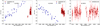 |
Fig. 1 Left panel: GJ 338 A HIRES (blue) and CARMENES (red) relative RV measurements at visible wavelengths. Middle panel: GJ 338 B HIRES (blue) and CARMENES (red) relative RV measurements at visible wavelengths. The time series data of each instrument has been normalized to a mean null velocity. Open circles indicate measurements that deviate more than 2σ from the observed velocity trend. Right panel: CARMENES relative RVs of GJ 338 B in the near-infrared. |
3.2 CARMENES radial velocity time series
We obtained new RVs for each member of the stellar binary using the CARMENES fibre-fed, échelle spectrograph. CARMENES is installed at the 3.5 m telescope of the Calar Alto Observatory in Almería (Spain). It was specifically designed to deliver high-resolution spectra at optical (resolving power R = 94 600) and near-infrared (R = 80 500) wavelengths covering from 520 to 1710 nm without any significant gap, using two different spectrograph arms: the VIS and NIR channels, respectively (Quirrenbach et al. 2016).
The CARMENES M-dwarf survey started in January 2016. The original sample of stars contained 324 M dwarfs (Caballero et al. 2016a; Reiners et al. 2018b,a), including GJ 338 B. Raw data are automatically reduced with the CARACAL pipeline (Caballero et al. 2016b). Relative radial velocities are extracted separately for the VIS and NIR channels using the SERVAL software (Zechmeister et al. 2018), which computes the average of all individually derived RVs order by order of the echélle observations. The results of the CARMENES planetary survey around M dwarfs reveal that the instrument is able to deliver time series of relative RVs with root mean square (rms) values of 3.5 and 9.0 m s−1 for the CARMENES VIS and NIR channels (Reiners et al. 2018a).
The systematic RV errors in spectral orders highly contaminated by telluric contribution, which is the case of CARMENES NIR data, can be increased by unmasked detector defects (Reiners et al. 2018a). Therefore, for the NIR channel, we carefully selected the orders that were included in the computation of the NIR RVs. These orders, selected to provide the smallest rms of the NIR RVs, were chosen after analyzing the entire CARMENES M-dwarf sample.
3.2.1 GJ 338 B
GJ 338 B is the main target of this paper. We used 159 CARMENES VIS and 120 NIR relative RVs obtained between 2016 January and2018 October. There are fewer NIR RVs because we selected only the NIR RVs taken after a technical intervention in the NIR channel in October 2016. GJ 338 B was observed with a typical cadence of one RV measurement every few to several days to sample short periodicities. All measurements employed in this work are provided in Tables B.1 (VIS) and B.2 (NIR). All data are corrected from barycentric motion, secular acceleration, instrumental drift, and nightly zero points (Trifonov et al. 2018). CARMENES VIS relative RVs of GJ 338 B as given in the CARMENES catalog of observations are depictedas a function of observing epoch in the middle panel of Fig. 1. The decreasing trend due to the orbital motion of the binary agrees with the trend delineated by the HIRES relative RVs. The right panel of Fig. 1 shows CARMENES NIR relative RVs of GJ 338 B. The slope of the NIR data is not as clear as that of the VIS RVs likely due to the larger uncertainties (and therefore, dispersion) of the NIR RVs.
3.2.2 GJ 338 A
The primary component of the stellar binary was also observed as part of the CARMENES M-dwarf program with a total of 70 RV measurements in the VIS channel taken between 2016 March and 2019 January. These VIS RVs, also relative and corrected from barycentric motion, secular acceleration, instrumental drift, and nightly zero points, are provided in Table B.3. GJ 338 A was not observed regularly at the beginning of the CARMENES M-dwarf project: the first three RVs were obtained more than one year before the remaining RV time series data. After 2017 December 18, GJ 338 A was monitored with a similar observing cadence as GJ 338 B. CARMENES VIS relative RVs are depicted as a function of observing epoch in the left panel of Fig. 1; they are shown together with the HIRES RV data of Tal-Or et al. (2019). Because the time coverage of the CARMENES data of GJ 338 A with a good time sampling is significantly shorter than that of GJ 338 B, we could not explore the same orbits as those of our study of GJ 338 B. These RVs were also used to study the orbital motion of the stellar pair (see Sect. 4.1) and to act as a reference (for its similarity in spectral type) in our search for low-mass planets around GJ 338 B.
3.3 Photometric time series
We obtained optical photometric time series of both GJ 338 A and B contemporaneous to the CARMENES data, aiming to derived the stellar rotational periods via the differential photometry technique. Images were acquired with telescopes of Las Cumbres Observatory Global Telescope (LCO, Brown et al. 2013) and Sierra Nevada Observatory (SNO). The 40-cm LCO telescopes used in our program are equipped with a 3k × 2k SBIG CCD camera with a pixel scale of 0′′.571 providing a field of view of 29.′2 × 19.′5. The 90-cm Ritchey-Chrétien SNO telescope has a VersArray 2k × 2k CCD camera with a square field of view of 13.′2 × 13.′2 (pixel scale of 0′′.39 on sky, Rodríguez et al. 2010). We applied a 2 × 2 binning to the detector. Raw frames were reduced following standard procedures at optical wavelengths, that is, bias subtraction and flat-field correction. Bad pixels were conveniently masked using well-tested masks provided by the observatories. In the case of LCO images, we used the banzai reduction products (McCully et al. 2018).
There were two photometric campaigns using LCO telescopes between 2018 March and 2019 February, and a third campaign using the SNO telescope from 2019 February to April. All three are summarized in Table 2, where we provide observing filters, the number of days covered per observing season, the number of photometric measurements, and the dispersion of the differential photometry. In the first photometric season, from 2018 March 5 to 27 (22 days of continuous monitoring), we acquired a total of 1800 and 2300 usable images of GJ 338 A and B using the V and i filters and a 2 × 2 binning of the detector. The on-source integration time was set at 1 s, and 100 consecutive images were typically acquired per filter and per night. On a few nights, the 100-frame sequence was acquired twice or three times. Weather conditions were variable from night to night as was also the seeing, with values varying between 1′′.0 and 5′′.0. The root-mean-square (rms) of the data are 14.4 mmag for the V -band light curve and 13.4 mmag for the i-band time series. The two light curves artificially normalized to zero magnitude are depicted in the top panels of Fig. 2.
In the second LCO campaign, from 2018 December through 2019 February (almost three months of continuous monitoring), we followed a slightly different observing strategy: between three and five images were typically obtained in the B and V filters throughout the observing nights resulting in more than 350 and 330 usable B- and V -band images whose differential photometry is shown in the middle panel of Fig. 2 (no normalization to zero magnitude was applied here). In this second season, the rms of the V -band light curve (10.7 mmag) is smaller than that of the first season. The third photometric season (2019 February22through April 13, that is, 50 days of nearly continuous monitoring) was acquired using the B and V filters immediately after the last LCO campaign. Typically, a total of 50 images were acquired with the SNO telescope per night. Exposure time changed between 6 and 20 s, depending on the seeing conditions. The SNO light curves are illustrated in the bottom panels of Fig. 2, and have an rms of 6.1 mmag (V) and 5.9 mmag (B). Also the LCO B-band light curve shows a smaller dispersion than the V -band data.
We used a circular apertures with radius of seven and 20 pixels to determine the LCO and SNO photometry of GJ 338 A and B, respectively. We checked that these apertures minimized the rms of the resulting light curves. The field of view registered by the LCO and SNO detectors is unfortunately devoid of bright stars that can act as reference sources for the differential photometry. Therefore, we derived the differential magnitude between the two components of the stellar binary (component B–component A). Because both stars share very similar spectral type, we did not apply any color correction to the differential photometry. With such a procedure, it is not possibleto discern which star is the source of any photometric variability, or if the two stars are variable simultaneously.
Given the large number of contemporaneous B, V, and i individual measurements available for both stellar components, we also derived differential B− V and V − i color light curves and found that GJ 338 A and B indeed show different colors, and that these colors appear rather stable throughout all monitoring campaigns. The relative color differences, although small, are significant in terms of the achieved photometric precision. GJ 338 B has B− V and V − i indices that are, on average, 12.5 ± 0.6 and 34.2 ± 0.7 mmag redder than those of GJ 338 A, where the error bars were obtained as the quadratically-summed photometric dispersions of both bands divided by the squared root of the number of measurements. These differences can be interpreted as both stars having slightly different temperatures (GJ 338 B would be cooler than GJ 338 A). Another possibility is a differing chemical composition of the stellar atmospheres (higher metallicity induces redder colors), but we give less credit to this scenario because the two stars are likely coeval and were probably formed from the same molecular cloud. GJ 338 B is also slightly fainter than the A component (ΔB = 110.2 ± 0.4, ΔV = 97.7 ± 0.6, and Δi = 65.6 ± 0.2 mmag), which combined with its redder nature may indicate that both stars have similar but not identical masses. The photometric properties of GJ 338 B (fainter and redder) suggest that this star is slightly less massive than GJ 338 A; this is compatible with the results presented in Sect. 4.1 but strongly disagrees with the mass derivations of Chang (1972).
GJ 338 A and B were also photometrically observed by the All-Sky Automated Survey for Supernovae survey (ASAS-SN, Kochanek et al. 2017). The ASAS-SN light curves show strong peak to peak variations. This behavior is far from what is seen in the LCO and SNO data. The ASAS-SN photometry was automatically derived from a 2-pixel radius aperture (i.e., about two FWHM in diameter) and the background was estimated from a 7–10 pixel radius annulus surrounding each of the two stars. The pixel scale of ASAS-SN detector is 8′′.0. Given the projected spatial separation of the stellar binary (ρ ~ 17′′.2), it becomes obvious that the ASAS-SN parameters for extracting the photometry of the system were not adequate and yield contaminated and useless light curves for GJ 338 A and B.
Photometric seasons available for GJ 338 A and B.
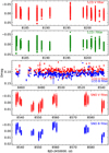 |
Fig. 2 Differential photometry (GJ 338 B–GJ 338 A) light curves obtained with the LCO and SNO telescopes. First and second panels: first photometric observing season covering a time interval of 22 days; third panel: light curve for the second observing season covering 87 days of continuous monitoring; and fourth and fifth panels: last observing season spanning 50 days. With the exception of the third panel, all photometry is artificially set to a mean value of zero magnitude. |
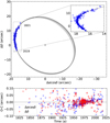 |
Fig. 3 Top panel: observed astrometric positions of GJ 338 B (blue dots) around the star GJ 338 A (black star located at 0,0 coordinates) expressed in Δδ vs. Δα cosδ. The black ellipse (dashed line) corresponds to the adopted Keplerian solution, which lies close to the region of the largest concentration of possible MCMC solutions. The oldest data and most recent astrometric data correspond to the year 1821 and 2019, respectively. Inner panel: zoom-in around the astrometric data. Only the adopted orbital solution is shown with the black dashed line. Bottom panel: residuals (± 0′′.11 in Δα cosδ and ± 0′′.14 in Δδ) after removing the adopted orbital solution plotted as a function of observing epoch (Δα cos δ: blue dots; Δδ: red dots). |
4 Analysis
4.1 Stellar binary orbital solution
In an attempt to constrain the orbital parameters of the stellar pair GJ 338 A and B, we considered all astrometric and spectroscopic data available to us in the pre-CARMENES era. As for the astrometry, we used theangular separations and position angles compiled by the Washington Double Star Catalog2 (WDS, Mason et al. 2001). This dataset provides astrometric measurements from mid 1821 through the first quarter of 2019. We completed the astrometric data using the SNO images from Sect. 3.3. By employing the 2MASS (Skrutskie et al. 2006)coordinates of all sources detected in the SNO frames, with the exception of the high proper motion targets GJ 338 A and B, we obtained the astrometric solution for seven different epochs in 2019, thus extending the time coverage of the Washington Double Star Catalog by two additional years. We found a plate scale of 0.388094 ± 0.000030 arcsec pix−1 (the pixels have the same length in the x- and y-axis within the quoted uncertainty) and that the SNO frames are 1.5 deg off the standard north–east orientation. This was corrected from the final measurements. We derived that the angular position of GJ 338 B with respect to the A component has changed by about 58 deg in 198 a of available astrometric observations. All astrometric data, including our latest derivations, in the form of angular separation (ρ) and position angle (θ) are given in Tables B.4 and B.5 and displayed in Fig. 3. As for the RVs, we used the ELODIE and HIRES absolute RVs of GJ 338 A and B as explained in Sect. 3.1.
To find the best Keplerian solution to the orbit of the stellar pair, and based on our knowledge of the system, any orbital solution has to reproduce the observed astrometric and radial velocity data and to be compliant with the following: (a) the total mass of the system should fall in the interval 1.03–1.38 M⊙, which is obtained from the 1σ smallest and largest individual values assigned to each component in Table B.1 of Schweitzer et al. (2019). According to these authors, the most likely total mass of the system is 1.187 ± 0.063 M⊙. (b) The two stellar components have very similar spectral type, effective temperature, magnitude, and luminosity (Passegger et al. 2018, 2019). Therefore, we expect the mass ratio, q, to be close to unity. In fact, Schweitzer et al. (2019) determined averaged masses of 0.591 ± 0.047 M⊙ for GJ 338 A and 0.596 ± 0.042 M⊙ for GJ 338 B (errors are also averaged from those given by the authors). These determinations were based on the analysis of CARMENES spectra and do not rely on astrometric or radial velocity observations.
The orbital parameters of the stellar pair GJ 338 A and GJ 338 B were obtained by simultaneously fitting the astrometric and RV data. Our code is based on PyMC3, which is a flexible and high-performance model building language and inference engine that scales well to problems with a large number of parameters, and on the exoplanet toolkit (e.g., Theano Development Team 2016), which extends PyMC3’s language to support many of the custom functions and distributions required when fitting our datasets (Salvatier et al. 2016). Exoplanet is also designed to provide the building blocks for fitting many datasets using the Markov chain Monte Carlo (MCMC) simulation approach. We set to 100 000 the number of MCMC simulations to derive the parameter distribution for the orbit of the binary; we allowed MCMC to explore values of orbital parameters in all possible ranges (e.g., eccentricity from 0.0 to almost 1.0), except for the orbital period and the amplitude of the RV curves, where we explored values in the intervals 800–5000 a and 0.4–5.0 km s−1. The posterior distributions of the fitted parameters are graphically shown in the corner plot of Fig. A.1, where it becomes apparent that the distribution of the solutions is narrow with clear peaks for most of the orbital parameters. The eccentricity distribution shows a peak at 0.0 with a long tail towards slightly larger values, yet our solution strongly indicates that the orbit is nearly circular with an eccentricity likely smaller than e = 0.1. More degenerated is the determination of the orbital inclination angle. This is not a surprising result because the available astrometric data cover less than 20% of the actual orbit of the stellar binary, which obviously is insufficient to find a tight solution.
Here, we adopted the orbital parameters mean values of the MCMC posterior distributions as the “best” Keplerian solution describing the observed astrometry and absolute RVs altogether. All adopted orbital parameters are given in Table 3. The mean values are very close to the peaks of the distributions shown in the corner plot of Fig. A.1. We found that the binary has a likely orbital period of 1295 ± 184 a, which is significantly larger than that of Chang (1972) but closer to the determination by Hopmann (1954), and a semi-major axis of 130.9 ± 5.1 au (or 20′′.66 ± 0′′.80). The error bars were determined by differenciating the various mean solutions obtained when removing data points from the long astrometric dataset. Figure 3 shows the observed astrometric positions of GJ 338 B around GJ 338 A between 1821 and 2019, the adopted Keplerian ellipse, and the residuals after removing the adopted orbital solution from the data. The residuals have a dispersion of ± 0′′.11 and ± 0′′.14 in right ascension (α) and declination (δ), respectively,which are close to the uncertainties of the best quality astrometry in our dataset. Furthermore, the residuals are flat over time, which indicates that the solution is acceptable for the covered time interval. With this solution, a total mass of 1.33 ± 0.17 M⊙ is obtained for the stellar pair, which is consistent at the 1σ level with the most likely value obtained by Schweitzer et al. (2019). The indivial mass of each binary component was then determined from the total mass and amplitude of the RV curves (mass ratio, q = KA∕KB = MB∕MA = 0.93 ± 0.13). We found dynamical masses of 0.69 ± 0.07 M⊙ for GJ 338 A and 0.64 ± 0.07 M⊙ for GJ 338 B.
Figure 4 shows the ELODIE and HIRES absolute RVs and the best Keplerian fit. The top panel illustrates 1.5 full orbital periods; the absolute RV data considered in this work cover a tiny fraction (<10 %) of the actual orbital period. The second and third panels of Fig. 4 show an enlargement of the previous panel centered on the observed velocities of GJ 338 A and B. Both the adopted Keplerian solution and a straight line fit to the RV data are included in the two panels. Given the small time coverage of the data, there is no perceptible difference between the Keplerian fit and the straight line (at the level of less than 1 m s−1, that is, about one order of magnitude smaller than the RV uncertainties). The fourth panel of Fig. 4 illustrates the velocity residuals (observations minus the fit), which have a dispersion of 11.13 (GJ 338 A) and 11.30 m s−1 (GJ 338 B).
As a consistency check of the quality of our adopted Keplerian fit, we produced the bottom panel of Fig. 4 that displays the differential velocity (vA − vB) of the binary members as a function of time using ELODIE, HIRES, SOPHIE, and CARMENES data, thus expanding the time coverage of the RV dataset by an additional 5.7 a for a total of 23.7 a. We assumed that the RV measurements of GJ 338 A and B are coeval if they were acquired on the same night or within a week time. With this condition, we identified 29 HIRES, 5 ELODIE, 39 SOPHIE, and 23 CARMENES RV pairs for GJ 338 A and B. This plot is in principle independent (or at least it minimizes the systematics) of the absolute RVs provided that all RVs are obtained using the same mask. For this purpose, we re-reduced all publicly available ELODIE, SOPHIE and CARMENES spectra using the SERVAL software (Zechmeister et al. 2018) and the same template of GJ 338 B for the two stars (Table B.6), thus removing the velocity zero point problem mentioned in Sect. 3.1. The adopted Keplerian solution nicely reproduces the differential velocity curve of the ELODIE and HIRES RVs and also extrapolates equally well towards the more recent SOPHIE and CARMENES data.
Another consistency check of the validity of the adopted Keplerian solution is given by the determination of the binary mass ratio through the measurement of the slopes of the combined ELODIE and HIRES RV curves of GJ 338 A and B. The mass ratio obtained in this way is q = 0.91 ± 0.11, which is compatible at the 1σ level with the value derived from the ratio of the RV amplitudes (KA, KB) of the adopted Keplerian fit.
Another method to derive the mass ratio of the binary is based on the equation q = (vA − γ)∕(γ − vB) (Wilson 1941), where γ stands for the systemic radial velocity. Because the mass ratio has to be a constant, we forced a flat (zero slope) q versus time as shown in Fig. 5. We employed the ELODIE and HIRES absolute RVs previously used in the Keplerian solution determination and enlarged the data coverage adding the CARMENES relative RVs calibrated to absolute value using the adopted Keplerian solution. The derived values are as follows: q = 0.930 ± 0.021, γ = 11.797 ± 0.001 km s−1. The small uncertainties associated with q and γ reflect the precision of the method, which leads to the conclusion that GJ 338 A is likely the most massive component of the stellar binary, as expected from its higher luminosity and bluer optical colors. This result is opposed to that of Chang (1972). By using the astrometric total mass of the stellar system, we obtained individual masses of 0.69 ± 0.03 M⊙ (GJ 338 A) and 0.64 ± 0.03 M⊙ (GJ 338 B), which are basically identical to the results from the first approach (combined astrometric and spectroscopic fit) and are consistent with the mass determinations by Schweitzer et al. (2019) at the 1σ level, but slightly larger by 8.3–9.4 % than those reported by these authors.
From now on, we use the stellar mass determinations from the combined astrometric and spectroscopic fit. Table 3 summarizes the derived orbital parameters, including the individual mass determinations and the mass ratio determinations from the spectroscopic data only.
Orbital parameters for the GJ 338 stellar binary system.
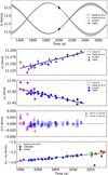 |
Fig. 4 First panel: radial velocity data and the joint astrometric and spectroscopic solution (black line) of the stellar binary system formed by GJ 338 A and GJ 338 B. The uncertainties are depicted with a gray color. ELODIE and HIRES absolute RVs are also shown. Second and third panels: zoom-in around the RVs of GJ 338 A and GJ 338 B, respectively. The straight line fit to the data is plotted as a green line. Given the high level of agreement between the adopted Keplerian solution and the straight line, the latter remains nearly hidden by the former in the two panels. Fourth panel: residuals of the RV observations minus the adopted Keplerian solution are shown with different symbols for the two stars. Bottom panel: ELODIE, HIRES, SOPHIE and CARMENES differential radial velocity curve (vA − vB) as a function of observing epoch. The values of the adopted Keplerian solution, which were fit using the ELODIE and HIRES data only, are shown with a black dashed line, errors in gray, and the straight line fit to the data is depicted with a green line. All four panels, from the second to the bottom one, have the same scale in the x-axis. |
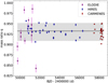 |
Fig. 5 Determination of the stellar mass ratio, q = MB∕MA, using ELODIE, HIRES, and CARMENES VIS differential radial velocities (see Sect. 4.1). The horizontal, solid line corresponds to q = 0.929 ± 0.019, where the uncertainty gray area accounts for the observed dispersion of the q values. |
4.2 RV detrending
Before investigating the presence of planets around each member of the GJ 338 stellar system, the Keplerian orbital solution (Table 3) was subtracted from the observed HIRES and CARMENES optical RVs. As a consistency check, we determined the negative (and positive) slope independently for the HIRES and CARMENES datasets, finding very similar results at the 1σ level. We concluded that given the short time coverage of the RV data and the long orbital period of the binary, the subtraction of a straight line instead of the Keplerian curve would not change the results reported next.
Our second step was to remove RV outliers from the GJ 338 B datasets by applying a 2σ-clipping algorithm, resulting in 1 HIRES RV and 6 CARMENES VIS RVs rejected from the lists of 32 and 159 independentmeasurements, respectively. Outliers typically have large error bars (due to, e.g., short exposures) and are marked in Fig. 1 and all other RV figures of this paper. The “flattened” and 2σ-clipping corrected CARMENES VIS RV dataset of GJ 338 B has a standard deviation of 4.2 m s−1, which is slightly smaller than the dispersion of the HIRES velocities (5.4 m s−1). The mean error bar value of the individual CARMENES VIS measurements provided by SERVAL is 2.4 m s−1, that is, almost a factor of two lower than the standard deviation. The origin of this RV excess variations is explored in the following section.
We also removed the orbital trend from the CARMENES NIR data of GJ 338 B and applied the 2σ-clipping for eliminating RV outliers after which we find a standard deviation of 9.2 m s−1. This value coincides with the typical dispersion of CARMENES NIR RVs of other M-type stars. Because of the larger rms of the NIR data, this channel does not deliver more convincing results than the VIS channel. Consequently, the NIR RVs were not used except when necessary.
The same procedure was applied to the CARMENES dataset of GJ 338 A resulting in the 2-σ-clipping removal of 4 VIS RVs out of a total of 70 measurements. The detrended RV curve of GJ 338 A has a standard deviation of 5.5 m s−1.
Besides RV precision, the cadence of the observations is also a critical ingredient for performing a proper analysis of temporal variability. In this regard, the CARMENES data were taken every few to several days while the target was visible from the Calar Alto Observatory. This observing frequency contrasts with the cadence of the HIRES observations (3–4 RV measurements per year). As a result, the CARMENES scheduled observations are ideal for exploring planets in short- to intermediate-period orbits (Garcia-Piquer et al. 2017), while the HIRES data are useful for identifying planets at longer orbital periods. Mixing the two datasets might not produce better results given the different data quality and temporal cadence. In what follows, we analyze the CARMENES VIS data independently and employ the HIRES and CARMENES NIR RVs to check the results.
4.3 Stellar activity
The profile of the stellar lines can be changed by photospheric and chromospheric activity, which has an impact on accurate RV measurements. M-type dwarfs typically have intense magnetic fields (Reiners et al. 2012, 2014; Newton et al. 2016, 2017; Shulyak et al. 2019), and it is expected that the related magnetic activity leaves a detectable trace in the high resolution spectra. Various groups have focused on the identification of spectral indicators of stellar activity (Montes et al. 2000; Gomes da Silva et al. 2011, 2012; Tal-Or et al. 2018) with the main goal of disentangling activity-induced RV variations and planetary signals. Two commonly-used chromospheric activity indicators are based on measurements of the Hα λ6562.82 Å and Ca II H and K λλ3933.7, 3968.5 Å lines. The blue Ca II H and K lines are not covered by the CARMENES data; instead, the Ca II infrared triplet λλλ8498, 8542, 8662 Å (IRT) is fully covered by the VIS channel. This triplet is also well known for its sensitivity to stellar activity as reported by Martínez-Arnáiz et al. (2011).
The CARMENES SERVAL pipeline provides measurements for a number of spectral features that can reveal stellar activity, including Hα, Ca II IRT, the differential line width (dLW), and the chromatic index (CRX), as defined by Zechmeister et al. (2018). The latter measures the RV– log λ correlation, and it is used as an indicator of the presence of stellar active regions. In addition, the pipeline computes the cross-correlation function (CCF) for each CARMENES spectrum using a weighted binary mask that was built from coadded observationsof the star itself. As explained by Reiners et al. (2018b), the CCFs are fitted with a Gaussian function to determine the contrast, the full width at half maximum (FWHM), and the bisector span (BIS), all of which are useful for studying stellar activity-related properties.
GJ 338 B
All CARMENES spectroscopic activity indicators of GJ 338 B are given in Table B.1. Their associated Generalized Lomb-Scargle periodograms (GLS; Zechmeister & Kürster 2009) are depicted in various panels of Fig. 6, where we also include the false alarm probability (FAP) levels of 10, 1, and 0.1% from 10 000 bootstrap randomizations of the input data. Peaks of the GLS periodograms with FAP level <0.1% are considered significant. The GLS method of analysis is particularly indicated for unevenly time series. With the exception of the CCF contrast, FWHM, and CRX indices, there is one single significant peak in all other activity indicators centered at ~0.060 d−1 (~16.6 d). The Ca II IRT and Hα indices folded in phase with this period are shown in Fig. 7: all of them have a sinusoid-like variation (dLW and BIS indices also show similar patterns).
We used the GLS peak at 16.6 d as the initial period for finding the best sinusoidal curve that minimizes the residuals of the activity indices presented in Fig. 7. We found that the best period is 16.61 ± 0.04 d, after averaging all individual determinations. We also checked that the variations of the activity indices do not correlate with the RVs. The shape of these variations and the fact that CRX and FWHM indices do not show the 16.6-d peak may be related to the origin and nature of the stellar variability that is inducing this signal in the CARMENES VIS RVs (see below and Schöfer et al. 2019). Hα and Ca II IRT are mainly chromospheric indicators while CRX is related to the photosphere. We ascribed the 16.6-d period to the chromospheric rotation cycle of GJ 338 B. This period determination differs from the values tabulated by Wright et al. (2011), who measured a photometric period of 10.17 d. However, later Fuhrmeister et al. (2019) reported a tentative period of 16.6 ± 0.5 d and 17.4 ± 1.0 d using CARMENES Hα and Ca II IRT activity indices, respectively. These values coincide with the 16.61 ± 0.04 d determined here and we agree with these authors that CARMENES Ca II IRT and Hα activity indices are well suited for stellar period searches.
As a side note, Abt & Levy (1973) measured the Ca II emission-line velocities of GJ 338 B and A and found them variable. They discussed that these variations were caused by the intrinsic multiple nature of each star, and determined a “binary” period of ~16.47 d for GJ 338 B (the one with the highest significance and amplitude of ~5 km s−1 according tothe authors). Later on, Morbey & Griffin (1987) obtained more data that did not confirm the proposed periods and did not suggest any variation in velocity at all, thus rejecting the notion that GJ 338 B is a binary star itself. The CARMENES RVs supportthis latter result. However, it is possible that Abt & Levy (1973) detected the rotation cycle of GJ 338 B because they were using emission lines very sensitive to stellar activity.
GJ 338 A
We analyzed the CARMENES VIS RVs of GJ 338 A in a similar manner as for the B component and found that the GLS periodograms of the Hα, dLW, and Ca II IRT activity indices (see Fig. 8) show a significant peak at 16.3 d (above FAP level <0.1 %). All RV and activity indices measurements are given in Table B.3. We verified that there is no confusion in the identification of the two stellar sources in the CARMENES catalog. The first evidence is that GJ 338 A RV data show a trend that is opposite to that of GJ 338 B, thus indicating that we are dealing with the two stellar components of the binary. The second piece of evidence is that the absolute RVs differ between the two stars. We attributed the periodicity of 16.3 d to the rotational cycle of GJ 338 A. Indeed, this rotation period is surprisingly close to that of GJ 338 B. It might hint that both M0-type stars, which were likely born from the same molecular cloud and are consequently coeval, have followed a very similar angular momentum evolution.
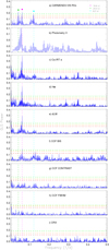 |
Fig. 6 GLS periodograms for GJ 338 B activity and RV data. In all panels, the horizontal dashed lines indicate FAP levels of 10% (red), 1% (orange), and 0.1% (green). Panel a: CARMENES RVs from the VIS channel. The three highest peaks at 8.3, 16.6, and 24.4 d are labeled and their positions are marked in all other panels with vertical dashed lines. Panel b: V -band photometry. Panels c–e: chromospheric line indices of the infrared Ca II triplet, Hα, and dLW. Panels f–h: FWHM, contrast, and bisector velocity span from the CCF analysis. Panel i: chromatic RV index (CRX). |
Photometry
For the present analysis, we studied the light curves separately per filter and per observing campaign and all seasons altogether (V -band data only, which is the only filter in common to the three campaigns). The differential light curve was obtained by dividing the fluxes of GJ 338 B and GJ 338 A because there is no other bright star in the field that can act as a reference source (see Sect. 3.3). The GLS periodogram of the entire V -band light curve is shown in the second panel (from the top) of Fig. 6, where a peak at around 18 d is detectable. The highest peaks in the GLS periodograms of the B- and i-band light curves lie between 16 and 20 d, but they are not significant. Also apparent in these periodograms is the peak at 8–10 d, which is likely due to the first harmonic of the primary signal. With the exception of the V -band data, we concluded that no obvious, significant peak can be extracted from the periodograms of the LCO and SNO light curves. From the analysis of the separated seasons of the V -filter data, we found a characteristic frequency in the interval 15.8–26.9 d, which covers the likely rotation periods of the two stars. The lack of an intense peak can be explained by photometric stability (or stellar variability that is below our detectability limit), by anti-correlated stellar variability of similar amplitude (thus producing a net amplitude close to zero in the differential light curve), or by the combination of two stellar variabilities of similar low amplitude and close, but not equal, periodicities, which could attenuate the true individual periodicities. The first hypothesis is the least likely one because there is stellar activity from the CARMENES spectroscopic data. With the current photometry, we could not discern the true scenario and therefore, we were not able to derive individual photometric periodicities for GJ 338 B and GJ 338 A.
4.4 Frequency content of the radial velocities of GJ 338 B
The GLS periodogram of the CARMENES VIS RVs of GJ 338 B is illustrated in the top panels of Figs. 6 and 9. The highest peak is located at ~24.4 d followed by two other significant peaks at ~8.3 and ~16.6 d. The three signals lie above FAP level 0.1 % and are marked in all panels of Figs. 6 and 9. The GLS periodogram of the CARMENES NIR RVs of GJ 338 B is shown in the second panel of Fig. 9. Only the peak at 16.6 d exceeds FAP ~ 10% (significance is not as high as in the optical probably because there are less NIR RVs and they have larger associated uncertainties). This signal at 16.6 d is common to all RV and many activity index GLS periodograms of GJ 338 B, and as discussed in the previous section, it is very likely related to the stellar rotation. Even though it is believed that the activity-induced signal is the strongest at blue wavelengths and is attenuated at long wavelengths in the RV time series (Martín et al. 2006; Huélamo et al. 2008), GJ 338 B clearly shows this peak in the near-infrared despite the larger error bars of the CARMENES NIR channel. This implies that the mechanism responsible for the activity in GJ 338 B is capable of imprinting its signal at both optical and near-infrared wavelengths. Figure 10 illustrates the CARMENES NIR RVs folded in phase with the rotation period of ~ 16.6 d; the curve shows a amplitude of 4.3 ± 1.7 m s−1.
For completeness, we also provide the GLS periodogram of the HIRES data of GJ 338 B in the third panel of Fig. 9. No significant signal is seen at any of the three peaks provided by the CARMENES VIS RV dataset. This is quite likely due to the insufficient cadence and long time coverage of the HIRES data. Interestingly, the combination of the HIRES and CARMENES VIS RVs recovers the 16.6 d signal well above FAP level 0.1% (fourth panel of Fig. 9). The second most prominent signal is located at ~24.4 d, which agrees with the results of the CARMENES VIS data.
In what follows, we demonstrate that the three signals (~8.3, ~16.6, and ~24.4 d) of the CARMENES VIS RVs of GJ 338 B are not related to each other by an aliasing effect, which is typically caused by the gaps in the time coverage of the observations (e.g., Dawson & Fabrycky 2010). To identify the presence of possible aliasing phenomena, the spectral window has to be considered. If peaks are seen in the window function, their corresponding aliases will be present in the RV periodograms as falias = ftrue ± mfwindow, where m is an integer, ftrue is the frequency identified in the RV periodogram and fwindow the frequency from the window function (Deeming 1975). Typical aliases are those associated with the sidereal year, synodic month, sidereal day, and solar day. The window function of the CARMENES VIS data is depicted in the top panel of Fig. 9 together with the GLS periodogram of the RVs. There are two significant peaks in the window function at the sidereal year and day. Using this information, we plotted the predicted aliases corresponding to each of the three significant peaks of theCARMENES VIS RVs in Fig. 11. From this figure, none of the three signals are related to each other by an alias of the observing window.
To summarize, based on the CARMENES VIS and NIR RV data we identified one strong signal at 16.61 ± 0.04 d, which is also significant in some activity indicators, and thus we relate it to the rotation period of GJ 338 B. The signals at ~8.3 and ~24.4 d do not havea counterpart in the activity indicators and are not aliases of the rotation signal. The ~8.3-d peak is exactly at half the rotation period, and we attribute it to the first harmonic of the stellar rotation. The ~24.4-d signal is notan exact multiple of the star’s rotation, and we attribute it to a planetary origin. We investigate its nature in Sect. 5.
To explore the stability of the ~24.4-d period, we produced the stacked periodogram of the CARMENES data shown in Fig. 12. For this purpose, we computed the Bayesian Generalized Lomb-Scargle periodogram (BGLS, Mortier et al. 2015). This formalism determines the probability between peaks of the periodogram. The signal at 24.4 d is very well detected with a probability above 1030 (with the minimum probability set to 1). This signal becomes more significant by adding observations as expected for a real signal.
 |
Fig. 7 GJ 338 B. Phase-folded time series of activity indicators Ca II λ8498 Å (left) and Hα λ6563 Å (right) and residuals. The solid curve depicts the best sinusoidal fit that modulates the rotation period at 16.6 d. |
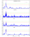 |
Fig. 8 GLS periodograms for GJ 338 A. In all panels, the horizontal dashed lines indicate FAP levels of 10% (red), 1% (orange), and 0.1% (green). Top panel: CARMENES VIS RVs. Second through fourth panels: CARMENES Ca II λ8498 Å, Hα, and dLW spectroscopic activity indicators. All activity indicators and the RV data show a significant, broad peak at around 16.3 |

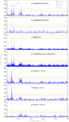 |
Fig. 9 GLS periodograms of the RV data of GJ 338 B. Panel a: periodogram of the CARMENES VIS RVs is plotted as a blue, solid line and the window function of the RV data is shown with an orange line. The three strongest signals are marked in this panel and in all other panels. The horizontal dashed lines indicate FAP levels of 10% (red), 1% (orange), and 0.1% (green). Panel b: peridogram of the CARMENES NIR RVs. Panel c: periodogram of the HIRES RV measurements. Panel d: periodogram of the combined HIRES + CARMENES VIS RV data. Panel e: periodogram of the CARMENES VIS RV residuals after removing the best-fit that modulates the stellar activity at Prot =16.6 d. Panel f: periodogram of the CARMENES VIS RV residuals after removing the stellar rotation and its first harmonic at 8.3 d. Panel g: periodogram of the CARMENES VIS RV residuals after removing all three significant signals. |
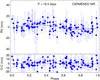 |
Fig. 10 Phase-folded CARMENES NIR RVs (blue dots) to 16.54 ± 0.06 d. Top panel: the black line depicts the best-fit that modulate the activity. Open circles stand for those points that deviate more than 2σ. The amplitude is 4.3 ± 1.7 m/s. Bottom panel: residuals’ rms is 7.5 m s−1. |
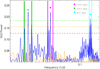 |
Fig. 11 Enlargement of the GLS periodogram of the CARMENES VIS RV data of GJ 338 B (blue line) around the three strongest signals (marked with color-coded dots). The window function is plotted as the orange line. Horizontal dashed lines indicate the different FAPs: 0.1% (green), 1% (orange) and 10% (red). The 1-sidereal-year aliases around each of the strongest signals are indicated with vertical solid lines. |
4.5 Frequency content of the radial velocities of GJ 338 A
The GLS periodogram of GJ 338 A CARMENES VIS RVs is illustrated in the top panel of Fig. 8. The highest peak is located at 16.3 d and shows abroad structure. No other signal lies above FAP 0.1%. As discussed in Sect. 4.3, this periodicity is also present in the GLS peridograms of the CARMENES activity indicators (Ca II IRT, Hα, and dLW) of GJ 338 A and it is very likely related to the stellar rotation.
This activity signal can be modeled by a periodic curve with an amplitude of 5.6 ± 0.7 m s−1 (VIS RV data). After its removal from the CARMENES VIS data, we found an rms of the residuals of 4.6 m s−1 and no additional significant peak in the corresponding periodogram above a FAP of 1%. We calculated the minimum mass of any putative planet around GJ 338 A in an orbital period range between 7 and 50 d using the third Kepler’s law, the mass of the parent star given in Table 1, and different values of eccentricity. The minimum period is given by four times the typical Nyquist frequency of the RV time series, and the maximum period is arbitrarily chosen. Figure 14 depicts the planetary minimum masses where we adopted, at the 1 σ level, the rms of the CARMENES VIS RVs multiplied by a factor of 0.92 as the minimum detectable RV amplitude. Bartlett et al. (2009) argued that a signal must be about 92% of the magnitude of the average residuals to be measurable through Lomb-Scargle-based periodograms. We are able to discard the presence of planets more massive than 10–19 M⊕ at 7–50 d orbits with eccentricity ~0.1, respectively.For more eccentric orbits, the planetary minimum masses decreases down to 8–14 M⊕ at 7–50 d orbits.
Following the same approach as for GJ 338 B (see Sect. 5), we also analyzed the GLS peridograms of the HIRES data and the combined HIRES+CARMENES VIS RVs of GJ 338 A, finding no characteristic frequency in the former and recovering the 16.3-d peak in the latter. The broad structure of the 16.3-d peak could be explained by the existence of differential rotation and/or blending of a real (very likely activity) signal at a similar period with an aliasing effect (due to one and two year aliases, time gaps between data, etc.). When removing the signal at 16.3 d from the HIRES+CARMENES dataset, another signal at 17 d became apparent above FAP 0.1% in the GLS periodogram of the residuals. Both 16.3 d and 17 d periodicitiesfall within the characteristic frequency interval of 15.8–26.9 d obtained from the analysis of the photometric V -band data. No more significant signals are present when removing the 16.3 d and 17 d periodic variations. Using current data, we cannot discard the presence of super-Earth or less massive planets “hidden" in the broad 16.3 d peak of the RV periodogram.
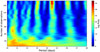 |
Fig. 12 Stacked BGLS periodogram for the CARMENES RVs data zoomed around the likely planetary orbital period of 24.4 days. The cumulative number of CARMENES observations is plotted as a function of periodicity; the color scale indicates the logarithm of the probability, where the red color stands for the most likely period. |
5 Planet orbiting GJ 338 B
5.1 Pre-whitening method
We obtained the best-fit orbital parameters of the planet at ~24.4 d using the RVLIN code3 (Wright & Howard 2009). This code is based on the Levenberg-Marquardt (Levenberg 1944; Marquardt 1963) algorithm and contains a set of routines that fits an arbitrary number of Keplerian curves to RV data. Our approach was as follows: first, we removed the“stellar contribution”, that is, activity, with a rotational period of 16.6 d from the observations by fitting a sinusoid function to the CARMENES VIS data. The fit, shown in the upper panel of Fig. 13, yielded an RV amplitude of 2.7 m s−1 (smaller than that obtained from the analysis of the NIR RVs, see Sect. 4.4). The residuals had an rms of 3.9 m s−1, which was slightly smaller than the initial standard deviation of the CARMENES VIS data, but still larger than the typical uncertainty associated with the individual RV measurements.
A new GLS periodogram of the residuals was obtained (it is depicted in panel e of Fig. 9). The planetary signal at ~24.4 d, which was also obvious in the original GLS periodogram, is now enhanced. The ~8.3 d peak still remains, although its significance is at the FAP level 10%. Because it is likely related to stellar activity, we removed its contributionfrom the VIS RV data by fitting a second sinusoid with a period of 8.26 d and and RV amplitude of 1.8 m s−1 (middle upper panel of Fig. 13). The new residuals have an rms of 3.6 m s−1. With these subsequent sinudoidal subtractions from the CARMENES VIS RV data, the only significal signal of the residuals has a characteristic period of 24.4 d (panel f of Fig. 9).
With the RVLIN code, we found the best Keplerian solution, which is illustrated in the third panel of Fig. 13, where the RV data are folded in phase with the planetary orbital period. The CARMENES VIS RV measurements that were not included in the analysis (open symbols in the RV plots) follow the trend and lie at the expected phases. The corresponding best-fit orbital parameters and their error bars are reported in Table 5. The best-fit orbital period is P = 24.40 ± 0.04 d, and the planet has a minimum mass of 9.2 ± 1.1 M⊕ (computed by adopting the mass of 0.64 ± 0.07 M⊙ for the parent star, as determined here). This planetary minimum mass would be 8.9 ± 1.2 M⊕ if the stellar mass determined by Schweitzer et al. (2019) were adopted instead. The planet candidate GJ 338 Bb is located at an orbital separation of 0.142 ± 0.014 au from its parent M0-type star, and despite its proximity, the planetary orbit appears to be slightly eccentric (e = 0.25 ± 0.13), although given the error bar of the eccentricity, the orbit is also compatible with an almost circular orbit. The amplitude of the planet RV curve is 2.8 ± 0.4 m s−1, about 38% smaller than the dispersion of the residuals data and similar to the mean error bar of individual CARMENES VIS RV data. The RV amplitudes of the stellar activity and the planet-induced signal are quite similar.
The RV residuals obtained after removing the stellar and planetary contribution from the CARMENES VIS RV data are shown in the bottom panel of Fig. 13. They have an rms of 3.0 m s−1, still larger than the mean error bar of individual RV measurements, but similar to the typical rms average of CARMENES data. The GLS periodogram of these residuals is displayed in panel g of Fig. 9; it shows no other significant peak. The results are not modified by changing the order of the pre-whitening method, thus giving robustness to the discovery of the small-mass planet around GJ 338 B. Table 5 summarises the orbtial parameters.
For completeness, we combined the CARMENES VIS and HIRES RV datasets of GJ 338 B. The fourth panel of Fig. 9 illustrates the corresponding GLS periodogram. We performed the same pre-whitening analysis as previously described. The amplitude of the stellar activity of the combined RV curve was determined at 2.7 m s−1, which fully agrees with that from the CARMENES-data only. The first residuals have an rms of 4.1 m s−1, which is indeed slightly higher than the first residuals of the CARMENES VIS RV data only. However, from this point of the analysis to the end of the process, the noise added by the HIRES data and the poor temporal coverage of this dataset prevented us from finding a consistent orbital solution (P = 24.40 d) despite the fact that the periodograms of the combined HIRES+CARMENES VIS RV residuals (not shown here) do not differ significantly from Fig. 9. The eccentricity value that we found for the planet orbital solution with the combined CARMENES VIS and HIRES RV data sets is e = 0.1. The lessons learnt from this exercise is that the HIRES RVs do not contradict the findings of the CARMENES data and that the eccentricity of the orbit of the planet around GJ 338 B is not well constrained with the current data.
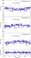 |
Fig. 13 CARMENES VIS RV data of GJ 338 B folded in phase with different periods. Each panel has been corrected for the others signals. Top panel: RV data folded in phase with the stellar rotation period of 16.6 d. Overplotted it is the best sinusoid function reproducing the data with an amplitude of 2.7 ± 0.5 m s−1. Second panel: RV folded in phase with the 8.3 d signal. Another sinusoid function is fit to these data with a RV amplitude of 1.8 ± 0.6 m s−1. Third panel: RV data folded in phase with the planetary orbital period of 24.4 d. The best Keplerian solution for the planet, with an RV amplitude of 2.8 ± 0.4 m s−1, is shown with the black line. Bottom panel: final RV residuals after removing the three signals (16.6, 8.3, and 24.4 d) have an rms = 3.0 m s−1. Open circles represent the RVs that deviate more than 2σ from the trend of the original data and that were not included in the analysis but are shown in this figure. |
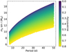 |
Fig. 14 Minimum detectable mass of any putative planet surrounding GJ 338 A as a function of the orbital period. We adopted the rms of the CARMENES VIS RV residuals as the amplitude of the Keplerian signals. The color code stands for the different values of the eccentricity. |
Comparison of different solutions for GJ 338 B.
5.2 Gaussian process regression method
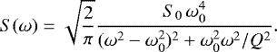
We also followed a different approach to study in detail the CARMENES VIS RV curve of GJ 338 B. This approach has the advantage of simultaneously fitting the stellar activity and the planetary signal(s). The match between the dominant period in dLW and Hα indices (Sect. 4.3) with one of the strongest signals in the RVs (Sect. 4.4) motivated a simultaneous fit of these activity indicators together with the RVs in order to account for the correlated RV noise. We used the celerite package (Foreman-Mackey et al. 2017) and its damped simple harmonic oscillator (SHO) kernel of the form
 (1)
(1)
The parameters of the model are the oscillator eigen-frequency (ω0), the quality factor (Q, corresponding to the inverse of the damping time scale), and the amplitude of the damped oscillator (S0). The former two are constrained by the activity indicator and an SHO Gaussian process (GP) kernel with these parameters, but with its own amplitude, is added to the planetary model. In addition to this, we used a model with individual offsets and RV jitter, as well as a linear trend, as the base line model (BM). The RV data and the activity indicators were then solved at the same time.
We used the Bayesian Information Criterion (BIC, Liddle 2007) to identify the optimal solution. When fitting models, it is possible to increase the log-likelihood (ln  ) by adding parameters, but the model may result in overfitting. The BIC resolves this problem by introducing a penalty term of the number of parameters in the model. It can be mathematically defined as follows:
 (2)
(2)
where n is the number of data points, k the number of free parameters to be estimated, and  the maximized value of the likelihood function of the model. The lower the BIC value, the better the model is.
In a first approach, we modeled the base model together with one SHO GP kernel (which picks the 16.6-d activity simultaneously in the RVs and in Hα or dLW), and the base model plus one planet with an orbital period of 24.4 d. With respect to the base model, these two models represented an improvement of the BIC value. Next, we explored how to lower the BIC parameter even further.
In the second approach, we modeled the base model, one Keplerian signal at 24.4 d, and one SHO GP kernel to account for the stellar activity with a cycle of 16.6 d. The fitted stochastic oscillator has a very high quality factor, that is, the life time is of the order of the duration of the observation. With this high quality factor, the GP kernel only acts in a very limited period/frequency range around its base frequency. The signal at 8.3 d (=1/2 Prot) is not removed. The planetary parameters of amplitude and orbital periodicity remained unaffected by the GP model.
In a third approach, we assumed that the peaks at 8.3 and 16.3 d are due to stellar rotation and the peak at 24.4 d is originated by a planet. We run the base model and added the planet and two SHO kernels that correspond to the stellar rotation period and its first harmonic (Prot/2). We forced the damping time of the two SHO kernels to be identical. The derived planetary parameters are compatible with the findings of previous models within the quoted error bars.
Our last approach consisted in treating the 8.3 d (Prot/2) signal as an additional Keplerian signal. This is, the base model, two planets at 8.3 and 24.4 d, and the stellar activity modeled with a SHO GP kernel at 16.6 d. Also this time, the planetary parameters of the 24.4-d planet remain unaffected. All models, including their priors, log-likelihood and BIC values, are summarized in Table 4.
According to the BIC criterion, the best solution for the CARMENES VIS RV curve of GJ 338 B is given by the base model, a SHO GP kernel modeling the stellar activity at 16.6 d, and two planets with orbital periods of 8.3 and 24.4 d (BM+GP+2pl in Table 4). The orbital parameters of the outermost planet are listed in Table 5. The 8.3-d planet would have the following derived parameters: minimum mass of 4.3 ± 1.5 M⊕ and semi-major axis of 0.067 ± 0.015 au. However, as mentioned in Sect. 4.4, the 8.3-d period is exactly half of the stellar rotation cycle; with the current data we cannot confirm the presence of this small planet around GJ 338 B. Therefore, we adopted the model given by the second approach, this is the base model, one SHO kernel for the stellar activity at the star’s rotation, and the planet at 24.4 d (BM+GP+1pl in Table 4). This is the solution for the GJ 338 B planetary system that we follow in this paper.
Summarizing, the eigen-frequency and the quality factor are converted to period and damping time, the uncertainties are derived from an MCMC procedure using emcee (Foreman-Mackey et al. 2013) with 200 walkers and 10 000 iterations after the burn-in phase. The autocorrelation length averaged over the walkers is 550, and the acceptance rate is 22% and during burn-in it is 35% (as described by Foreman-Mackey et al. 2013). We also checked the chains of each parameter as a function of the step and after the burn-in phase, and the walkers were wandering around the best parameter. The MCMC posterior distributions for the fitted parameters are presented in Fig. A.2. The derived orbital parameters using the GP regression are reported in Table 5 and they are compatible within the quoted error bars with the values obtained in the previous section using the pre-whitening approach and the RVLIN code.
In the top-left panel of Fig. 15, the solution combining stellar activity (as measured from the Hα index, see right panels of Fig. 15) and the planetary signal is depicted as a function of time (with an arbitrary zero date). The stellar activity was modeled with a damped oscillator with a period of 16.6 d and a long damping time scale of about 250 d. The weighted rms of the CARMENES VIS RVs after model subtraction is 3.2 m s−1, and 0.0084 for the Hα index. The CARMENES VIS RV residuals are illustrated in the second panel of Fig. 15, while the third and four panels stand for the GLS periodograms of the RV original and residual data as a function of frequency and period. The RV data and the residuals folded in phase at the best Keplerian solution obtained with the GP regression are illustrated in Fig. 16. The RV amplitude of Keplerian signal is 3.07 ± 0.37 m s−1.
Keplerian orbital parameters of GJ 338 Bb from pre-whitening and Gaussian process regresion methods.
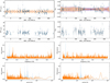 |
Fig. 15 Left panels, top panel: CARMENES VIS RVs (blue dots) together with a Keplerian model combined with a simple-harmonic oscillator (SHO) model shown in orange. The Keplerian-only curve is shown with a light blue color. Second panel: RV residuals after subtracting the combined Keplerian + simple-harmonic oscillator model from the original data. Third and bottom panels: GLS periodograms of the original data (light blue line) and of the RV residuals (orange) as a function of frequency and period. The model accounts for the two strongest peaks at 16.6 d and 24.4 d. Right panels: CARMENES Hα data compared to a simple harmonic oscillator (SHO) model (see Sect. 5.2) and the residuals (top two panels), as well as the periodogram as a function of frequency and period (lower two panels). Top panel: best fit model is shown in orange, the 1σ uncertainty in blue. The periodograms show the data in light blue and the residuals in orange. |
6 Discussion
The two stars are very similar in mass, spectral type, brightness, and even rotation period, but they appear to differ in the architecture of their planetary systems. Given the rotation period of GJ 338 B (16.61 ± 0.04 d), its projected rotational velocity (v sin i = 2.3 ± 1.5 km s−1), and the star’s radius (0.58 ± 0.03R⊙) as taken from the literature, it is not possible to determine a precise inclination angle of the stellar rotation angle. It is likely that the projected rotational velocity is smaller than the values published in the literature. The rotation period agrees with the observed relation between X-ray luminosity and stellar activity or rotation from, for example, Wright et al. (2011).
Here, we have used two mass determinations for the M0V-type star GJ 338 B. One was obtained from the most likely astrometric solution of the stellar binary combined with the mass ratio determination from absolute radial velocity measurements. This value (Table 3) is fully independent of any evolutionary model and mass-luminosity calibrations. Despite the degeneracy of the astrometric solution (Sect. 4.1), the individual masses of the stellar components are well constrained. The second measurement provided by Schweitzer et al. (2019) is based on various well known calibrations that are valid for low-mass stars. The two determinations differ by less than 10%, thus having little impact in the mass determination of the planet orbiting this star.
The top panel of Fig. 17 shows the location of GJ 338 Bb in the planetary minimum mass versus planetary orbital period diagram together with other Neptune-size and super-Earth planets known around M-type dwarfs. Our planet does not stand out in this diagram, neither it does when we select only those planets that are orbiting one of the stars of the binary systems (S-type configuration; Rabl & Dvorak 1988). The bottom panel of Fig. 17 displays such comparison, where we included the ~70 discovered planets in S-type configuration with stellar projected physical separations s ≤ 1000 au and known planet orbital periods and minimum masses. The majority of these planets have been identified around stars in binary systems with large physical separation, typically mean values s > 400 au. GJ 338 Bb is one of the least massive planets identified in one component of a stellar binary with separation well below of 400 au. The super-Earth planet around GJ 338 B adds to the increasing list of planets orbiting one of the stars of stellar binary systems. Weremark the similarity of the two stellar components of the GJ 338 binary and also provide various existing examples with very similar components such as: WASP-2 AB, XO-2N, XO-2S, HD 177830 AB, Kepler 296 AB, WASP-94 AB and Gliese 15 AB (Collier Cameron et al. 2007; Torres et al. 2008; Meschiari et al. 2011; Desidera et al. 2014; Rowe et al. 2014; Neveu-VanMalle et al. 2014; Pinamonti et al. 2018).
Following commonly used expressions (e.g., Borucki & Summers 1984; Sackett 1999; Stevens & Gaudi 2013), we derived the probability that GJ 338 Bb transits in front of the disk of its parent star to be 5 %. Using the unbiased forecasting model presented by Chen & Kipping (2017), we predict the planetary radius to be
  ; with this, the depth of any putative transit signal would be 0.24
 % as computed for a planetary mass of
  M⊕. TESS observed the GJ 338 binary system in sector 21 between 2020 January 21 and February 18. Due to the pixel scale of TESS (21″/pixel), the two stars GJ 338 A and B are not resolved.
We adopted the traditionally defined habitable zone as the circumstellar region in which a terrestial-mass planet with a CO2–H2O–NO2 atmosphere can sustain liquid water on its surface (Selsis et al. 2007). We estimated the theoretical equilibrium temperature of GJ 338 Bb by using the Stefan–Boltzmann equation, the stellar parameters of Table 1, and two extreme values of the albedo (A = 0.0 and 0.65; the highest albedo corresponds to the case of Venus in our Solar System). The results are Teq = 391 ± 20 K for a non-reflecting planet and 301 ± 20 K for the high-reflectance planet. The error bars come from the uncertainties in the stellar luminosity and semi-major axis of the planet. Kopparapu et al. (2013) calculated conservative and optimistic estimates of the habitable zone (water-loss and maximum greenhouse limits); by using their determinations of the boundaries of the habitable zone, we found them to be in the interval 0.29–0.57 au around GJ 338 B. This implies that the planet GJ 338 Bb lies inside the inner boundary of the habitable zone which is consistent with the hot equilibrium temperature estimated above. Previous works (e.g., Kasting et al. 1993; Rodríguez et al. 2012; Barnes 2017) established that low-mass stellar hosts can induce strong tidal effects on potentially habitable planets since they tend to be on close-in orbits. True planet habitability may be compromised for planets orbiting within the tidal lock radius of the star. Figure 16 reported by Kasting et al. (1993) shows the tidal lock radius for various stellar spectral classes, including M0 V. From this figure, it becomes apparent that GJ 338 Bb is very likely tidally locked given its short orbit.
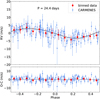 |
Fig. 16 Top panel: planetary signal of GJ 338 B CARMENES VIS RVs (blue dots) folded in phase with the orbital period derived from the GP regression analysis (the base model and the stellar activity were removed). The best Keplerian solution (black line) has an RV amplitude of 3.07 ± 0.37 m s−1. The red dots correspond to the binned data. Bottom panel: RV residuals after the subtraction of the model. The weighted rms of the residuals is 3.2 m s−1. |
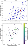 |
Fig. 17 Top panel: planetary minimum mass vs. orbital period for known Neptune-sized and super-Earth planets (blue dots) around M dwarfs. The planet GJ 338 Bb is plotted as the red star symbol. Bottom panel: planetary minimum mass versus semi-major axis for all known planets (color dots) in S-type configuration around binary systems, where the stellar binaries have projected physical separation s ≤ 1000 au (color bar). The stellar binary separation between the A and B members of our binary system has a semi-major axis of 130.9au and is plotted as star symbol. |
7 Conclusions
With the CARMENES spectrograph, we monitored the very bright M0.0 V stars GJ 338 B (HD 79211) and GJ 338 A (HD 79210), which form a wide binary in the nearby solar vicinity. We also provided a refined astrometric and spectroscopic solution of the stellar binary orbit by using all data from the literature available to us. The adopted Keplerian solution for the two stars yielded an orbital period of 1295 a and a semi-major axis of 130.9 au. The orbital period value reported here is significantly larger than those previously given in the literature (e.g., Chang 1972). Despite the great similarity between the two stars, we determined slightly different mass values for the A and B stellar components (0.69 ± 0.07 and 0.64 ± 0.07 M⊙, respectively), suggesting that the A stellar member is about 7% more massive than the B component. Furthermore, they are also consistent with the masses derived by Schweitzer et al. (2019).
All activity indicators provided by CARMENES VIS data (Ca II infrared triplet, Hα line, chromatic spectral index, the differential line width and cross correlation function analysis), together with the new photometry acquired by our group at LCO and SNO, indicate that GJ 338 B and A are active stars and rotate with periodicities of P = 16.61 ± 0.04 d and P = 16.3 d, respectively,which agrees with the expected X-ray luminosity–activity relations.
The detailed analysis of CARMENES RVs led to the discovery of a super-Earth planet orbiting GJ 338 B with an orbital period of 24.45 ± 0.02 d, and a minimum mass of 10.27 M⊕, and a semi-major axis of 0.141 ± 0.005 au. Another period was found in the CARMENES RV data at ~8.3 d, but without sufficient number of arguments to prove its Keplerian nature and because it lies at half of the stellar rotation period, we attributed it to the first harmonic of the stellar activity. A related analysis concluded that GJ 338 A does not have planets of similar massor more massive than GJ 338 Bb. The majority of the stellar binary systems with planet hosts have larger separations than the pair GJ 338 A and B and their planets are also larger in mass than GJ 338 Bb. Therefore, GJ 338 Bb has become one of the least massive planets ever discovered in one star of a binary system of relatively small separation.
Acknowledgements
We wish to thank the anonymous referee for helpful comments and suggestions, which helped to improve the manuscript. We are grateful to Prof. B. D. Mason for providing Washington Double Star astrometric data for the stellar binary. Based on observations collected at the German-Spanish Astronomical Center, Calar Alto, jointly operated by the Junta de Andalaucía and the Instituto de Astrofísica de Andalucía (CSIC), andobservations from Las Cumbres Observatory Global Telescope (LCOGT) network. LCOGT observations were partially acquired via program number TAU2019A-002 of the Wise Observatory, Tel-Aviv University, Israel. CARMENES is an instrument for the Centro Astronómico Hispano-Alemán de Calar Alto (CAHA, Almería, Spain). CARMENES is funded by the German Max-Planck- Gesellschaft (MPG), the Spanish Consejo Superior de Investigaciones Científicas(CSIC), the European Union through FEDER/ERF funds, and the members of the CARMENES Consortium (Max-Planck-Institut für Astronomie, Instituto de Astrofísica de Andalucía, Landessternwarte Koönigstuhl, Institut de Ciències de l’Espai, Insitut für Astrophysik Göttingen, Universidad, Complutense de Madrid, Thüringer Landessternwarte Tautenburg, Instituto de Astrofísica de Canarias, Hamburger Sternwarte, Centro de Astrobiología and Centro Astronómico Hispano-Alemán), with additional contributions by the Spanish Ministry of Economy, the state of Baden-Wüttemberg, the German Science Foundation (DFG), the Klaus Tschira Foundation (KTS), and by the Junta de Andalucía. This work is supported by the Spanish Ministery for Science, Innovation, and Universities through projects AYA-2016-79425-C3-1/2/3-P, AYA2015-69350-C3-2-P, ESP2017-87676-C5-2-R, ESP2017-87143-R. The Instituto de Astrofísica de Andalucía is a Centre of Excellence “Severo Ochoa” (SEV-2017-0709). The Centro de Astrobiología (CAB, CSIC-INTA) is a Center of Excellence “Maria de Maeztu”.
Appendix A Additional figures
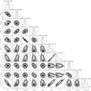 |
Fig. A.1 MCMC distribution of the combined astrometric and spectroscopic analysis of the GJ 338 AB binary system. The vertical dashed lines indicate the 16, 50, and 84% quantiles of the fitted parameters; this corresponds to 1 σ uncertainty. The reference time of T0 distribution is 2 200 000. |
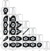 |
Fig. A.2 MCMC distribution of the planet orbiting GJ 338 B. The vertical dashed lines indicate the 16, 50, and 84% quantiles of the fitted parameters; this corresponds to 1 σ uncertainty. The best fit is colored. |
Appendix B Additional tables
Full Tables B.1–B.6 are only available at the CDS.
GJ 338 B data of the CARMENES observations.
Relative radial velocity measurements of GJ 338 B with CARMENES in the NIR.
GJ 338 A data of the CARMENES observations.
Relative astrometric position of the binary companion GJ 338 B to GJ 338 A.
Relative and differential RVs for binary GJ338AB computed with common template (GJ338B).
References
- Abt, H. A., & Levy, S. G. 1973, AJ, 78, 1093 [NASA ADS] [CrossRef] [Google Scholar]
- Affer, L., Damasso, M., Micela, G., et al. 2019, A&A, 622, A193 [NASA ADS] [CrossRef] [EDP Sciences] [Google Scholar]
- Alonso-Floriano, F. J., Morales, J. C., Caballero, J. A., et al. 2015, A&A, 577, A128 [NASA ADS] [CrossRef] [EDP Sciences] [Google Scholar]
- Anglada-Escudé, G., Arriagada, P., Vogt, S. S., et al. 2012, ApJ, 751, L16 [NASA ADS] [CrossRef] [Google Scholar]
- Astudillo-Defru, N., Bonfils, X., Delfosse, X., et al. 2015, A&A, 575, A119 [NASA ADS] [CrossRef] [EDP Sciences] [Google Scholar]
- Baranne, A., Queloz, D., Mayor, M., et al. 1996, A&AS, 119, 373 [NASA ADS] [CrossRef] [EDP Sciences] [Google Scholar]
- Barnes, R. 2017, Celest. Mech. Dyn. Astron., 129, 509 [Google Scholar]
- Bartlett, J. L., Ianna, P. A., & Begam, M. C. 2009, PASP, 121, 365 [NASA ADS] [CrossRef] [Google Scholar]
- Beavers, W. I., & Eitter, J. J. 1986, ApJS, 62, 147 [NASA ADS] [CrossRef] [Google Scholar]
- Bonfils, X., Lo Curto, G., Correia, A. C. M., et al. 2013, A&A, 556, A110 [NASA ADS] [CrossRef] [EDP Sciences] [Google Scholar]
- Bopp, B. W., & Meredith, R. 1986, PASP, 98, 772 [NASA ADS] [CrossRef] [Google Scholar]
- Borucki, W. J., & Summers, A. L. 1984, Icarus, 58, 121 [NASA ADS] [CrossRef] [Google Scholar]
- Boyajian, T. S., von Braun, K., van Belle, G., et al. 2012, ApJ, 757, 112 [NASA ADS] [CrossRef] [Google Scholar]
- Brown, T. M., Baliber, N., Bianco, F. B., et al. 2013, PASP, 125, 1031 [NASA ADS] [CrossRef] [Google Scholar]
- Butler, R. P., Vogt, S. S., Laughlin, G., et al. 2017, AJ, 153, 208 [NASA ADS] [CrossRef] [Google Scholar]
- Caballero, J. A., Cortés-Contreras, M., Alonso-Floriano, F. J., et al. 2016a, in 19th Cambridge Workshop on Cool Stars, Stellar Systems, and the Sun (CS19), 148 [Google Scholar]
- Caballero, J. A., Guàrdia, J., López del Fresno, M., et al. 2016b, Proc. SPIE, 9910, 99100E [Google Scholar]
- Carleo, I., Benatti, S., Lanza, A. F., et al. 2018, A&A, 613, A50 [NASA ADS] [CrossRef] [EDP Sciences] [Google Scholar]
- Chang, K. 1972, AJ, 77, 759 [NASA ADS] [CrossRef] [Google Scholar]
- Chen, J., & Kipping, D. 2017, ApJ, 834, 17 [Google Scholar]
- Claudi, R., Benatti, S., Carleo, I., et al. 2017, Eur. Phys. J. Plus, 132, 364 [CrossRef] [Google Scholar]
- Collier Cameron, A., Bouchy, F., Hébrard, G., et al. 2007, MNRAS, 375, 951 [NASA ADS] [CrossRef] [Google Scholar]
- Cortés-Contreras, M. 2016, PhD thesis, Universidad Complutense de Madrid, Spain [Google Scholar]
- Cortés-Contreras, M., Béjar, V. J. S., Caballero, J. A., et al. 2017, A&A, 597, A47 [NASA ADS] [CrossRef] [EDP Sciences] [Google Scholar]
- Damasso, M., Bonomo, A. S., Astudillo-Defru, N., et al. 2018, A&A, 615, A69 [NASA ADS] [CrossRef] [EDP Sciences] [Google Scholar]
- Dawson, R. I., & Fabrycky, D. C. 2010, ApJ, 722, 937 [NASA ADS] [CrossRef] [Google Scholar]
- Deeming, T. J. 1975, Ap&SS, 36, 137 [NASA ADS] [CrossRef] [MathSciNet] [Google Scholar]
- Desidera, S., Bonomo, A. S., Claudi, R. U., et al. 2014, A&A, 567, L6 [NASA ADS] [CrossRef] [EDP Sciences] [Google Scholar]
- Díez Alonso, E., Caballero, J. A., Montes, D., et al. 2019, A&A, 621, A126 [NASA ADS] [CrossRef] [EDP Sciences] [Google Scholar]
- Dressing, C. D., & Charbonneau, D. 2013, ApJ, 767, 95 [NASA ADS] [CrossRef] [Google Scholar]
- Dressing, C. D., & Charbonneau, D. 2015, ApJ, 807, 45 [NASA ADS] [CrossRef] [Google Scholar]
- Eiroa, C., Marshall, J. P., Mora, A., et al. 2013, A&A, 555, A11 [NASA ADS] [CrossRef] [EDP Sciences] [Google Scholar]
- Foreman-Mackey, D., Hogg, D. W., Lang, D., & Goodman, J. 2013, PASP, 125, 306 [CrossRef] [Google Scholar]
- Foreman-Mackey, D., Agol, E., Ambikasaran, S., & Angus, R. 2017, AJ, 154, 220 [NASA ADS] [CrossRef] [Google Scholar]
- Fuhrmeister, B., Czesla, S., Schmitt, J. H. M. M., et al. 2019, A&A, 623, A24 [NASA ADS] [CrossRef] [EDP Sciences] [Google Scholar]
- Gagné, J., Plavchan, P., Gao, P., et al. 2016, ApJ, 822, 40 [NASA ADS] [CrossRef] [Google Scholar]
- Gaia Collaboration (Brown, A. G. A., et al.) 2018, A&A, 616, A1 [NASA ADS] [CrossRef] [EDP Sciences] [Google Scholar]
- Gaidos, E., & Mann, A. W. 2014, ApJ, 791, 54 [NASA ADS] [CrossRef] [Google Scholar]
- Gaidos, E., Mann, A. W., Lépine, S., et al. 2014, MNRAS, 443, 2561 [NASA ADS] [CrossRef] [Google Scholar]
- Gaidos, E., Mann, A. W., Kraus, A. L., & Ireland, M. 2016, MNRAS, 457, 2877 [NASA ADS] [CrossRef] [Google Scholar]
- Garcia-Piquer, A., Morales, J. C., Ribas, I., et al. 2017, A&A, 604, A87 [NASA ADS] [CrossRef] [EDP Sciences] [Google Scholar]
- Głȩbocki, R., & Gnaciński, P. 2005, ESA SP, 560, 571 [NASA ADS] [Google Scholar]
- Gomes da Silva, J., Santos, N. C., Bonfils, X., et al. 2011, A&A, 534, A30 [NASA ADS] [CrossRef] [EDP Sciences] [Google Scholar]
- Gomes da Silva, J., Santos, N. C., Bonfils, X., et al. 2012, A&A, 541, A9 [NASA ADS] [CrossRef] [EDP Sciences] [Google Scholar]
- Güntzel-Lingner. 1954, IAU Commission Binary and Multiple Star Systems Information Bulletin, 4 [Google Scholar]
- Hartkopf, W. I., Mason, B. D., & Worley, C. E. 2001, AJ, 122, 3472 [NASA ADS] [CrossRef] [Google Scholar]
- Hartman, J. D., Gaudi, B. S., Pinsonneault, M. H., et al. 2009, ApJ, 691, 342 [NASA ADS] [CrossRef] [Google Scholar]
- Hartman, J. D., Bakos, G. Á., Kovács, G., & Noyes, R. W. 2010, MNRAS, 408, 475 [NASA ADS] [CrossRef] [Google Scholar]
- Henry, T. J., Jao, W.-C., Subasavage, J. P., et al. 2006, AJ, 132, 2360 [NASA ADS] [CrossRef] [Google Scholar]
- Hopmann. 1954, IAU Commission Binary and Multiple Star Systems Information Bulletin, 3 [Google Scholar]
- Howard, A. W., Marcy, G. W., Bryson, S. T., et al. 2012, ApJS, 201, 15 [NASA ADS] [CrossRef] [Google Scholar]
- Huélamo, N., Figueira, P., Bonfils, X., et al. 2008, A&A, 489, L9 [NASA ADS] [CrossRef] [EDP Sciences] [Google Scholar]
- Isaacson, H., & Fischer, D. 2010, ApJ, 725, 875 [NASA ADS] [CrossRef] [Google Scholar]
- Jenkins, J. S., Ramsey, L. W., Jones, H. R. A., et al. 2009, ApJ, 704, 975 [NASA ADS] [CrossRef] [Google Scholar]
- Kaminski, A., Trifonov, T., Caballero, J. A., et al. 2018, A&A, 618, A115 [NASA ADS] [CrossRef] [EDP Sciences] [Google Scholar]
- Kasting, J. F., Whitmire, D. P., & Reynolds, R. T. 1993, Icarus, 101, 108 [NASA ADS] [CrossRef] [PubMed] [Google Scholar]
- Kiselev, A. A., & Kiyaeva, O. V. 1980, AZh, 57, 1227 [NASA ADS] [Google Scholar]
- Kiselev, A. A., & Romanenko, L. G. 1996, Astron. Rep., 40, 795 [NASA ADS] [Google Scholar]
- Kochanek, C. S., Shappee, B. J., Stanek, K. Z., et al. 2017, PASP, 129, 104502 [NASA ADS] [CrossRef] [Google Scholar]
- Kopparapu, R. K., Ramirez, R., Kasting, J. F., et al. 2013, ApJ, 765, 131 [NASA ADS] [CrossRef] [Google Scholar]
- Leto, G., Pagano, I., Buemi, C. S., & Rodono, M. 1997, A&A, 327, 1114 [NASA ADS] [Google Scholar]
- Levenberg, K. 1944, Q. Appl. Math., 2, 164 [Google Scholar]
- Liddle, A. R. 2007, MNRAS, 377, L74 [NASA ADS] [Google Scholar]
- Luque, R., Nowak, G., Pallé, E., et al. 2018, A&A, 620, A171 [NASA ADS] [CrossRef] [EDP Sciences] [Google Scholar]
- Luque, R., Pallé, E., Kossakowski, D., et al. 2019, A&A, 628, A39 [NASA ADS] [CrossRef] [EDP Sciences] [Google Scholar]
- Malkov, O. Y., Tamazian, V. S., Docobo, J. A., & Chulkov, D. A. 2012, A&A, 546, A69 [NASA ADS] [CrossRef] [EDP Sciences] [Google Scholar]
- Marquardt, D. 1963, SIAM J. Appl. Math., 11, 431 [Google Scholar]
- Martín, E. L., Guenther, E., Zapatero Osorio, M. R., Bouy, H., & Wainscoat, R. 2006, ApJ, 644, L75 [NASA ADS] [CrossRef] [Google Scholar]
- Martínez-Arnáiz, R., Maldonado, J., Montes, D., Eiroa, C., & Montesinos, B. 2010, A&A, 520, A79 [NASA ADS] [CrossRef] [EDP Sciences] [Google Scholar]
- Martínez-Arnáiz, R., López-Santiago, J., Crespo-Chacón, I., & Montes, D. 2011, MNRAS, 414, 2629 [NASA ADS] [CrossRef] [Google Scholar]
- Mason, B. D., Wycoff, G. L., Hartkopf, W. I., Douglass, G. G., & Worley, C. E. 2001, AJ, 122, 3466 [Google Scholar]
- McCully, C., Volgenau, N. H., Harbeck, D.-R., et al. 2018, SPIE Conf. Ser., 10707, 107070K [Google Scholar]
- Meschiari, S., Laughlin, G., Vogt, S. S., et al. 2011, ApJ, 727, 117 [NASA ADS] [CrossRef] [Google Scholar]
- Montes, D., Fernández-Figueroa, M. J., De Castro, E., et al. 2000, A&AS, 146, 103 [NASA ADS] [CrossRef] [EDP Sciences] [Google Scholar]
- Morales, J. C., Mustill, A. J., Ribas, I., et al. 2019, Science, 365, 1441 [NASA ADS] [CrossRef] [Google Scholar]
- Morbey, C. L., & Griffin, R. F. 1987, ApJ, 317, 343 [NASA ADS] [CrossRef] [Google Scholar]
- Mortier, A., Faria, J. P., Correia, C. M., Santerne, A., & Santos, N. C. 2015, A&A, 573, A101 [NASA ADS] [CrossRef] [EDP Sciences] [Google Scholar]
- Morton, T. D., & Swift, J. 2014, ApJ, 791, 10 [NASA ADS] [CrossRef] [Google Scholar]
- Moutou, C., Hébrard, E. M., Morin, J., et al. 2017, MNRAS, 472, 4563 [NASA ADS] [CrossRef] [Google Scholar]
- Mulders, G. D., Pascucci, I., & Apai, D. 2015, ApJ, 798, 112 [Google Scholar]
- Nagel, E., Czesla, S., Schmitt, J. H. M. M., et al. 2019, A&A, 622, A153 [NASA ADS] [CrossRef] [EDP Sciences] [Google Scholar]
- Neves, V., Bonfils, X., Santos, N. C., et al. 2013, A&A, 551, A36 [NASA ADS] [CrossRef] [EDP Sciences] [Google Scholar]
- Neveu-VanMalle, M., Queloz, D., Anderson, D. R., et al. 2014, A&A, 572, A49 [NASA ADS] [CrossRef] [EDP Sciences] [Google Scholar]
- Newton, E. R., Irwin, J., Charbonneau, D., Berta-Thompson, Z. K., & Dittmann, J. A. 2016, ApJ, 821, L19 [NASA ADS] [CrossRef] [Google Scholar]
- Newton, E. R., Irwin, J., Charbonneau, D., et al. 2017, ApJ, 834, 85 [NASA ADS] [CrossRef] [Google Scholar]
- Nidever, D. L., Marcy, G. W., Butler, R. P., Fischer, D. A., & Vogt, S. S. 2002, ApJS, 141, 503 [NASA ADS] [CrossRef] [Google Scholar]
- Osten, R. A., Hawley, S. L., Allred, J. C., Johns-Krull, C. M., & Roark, C. 2005, ApJ, 621, 398 [NASA ADS] [CrossRef] [Google Scholar]
- Passegger, V. M., Reiners, A., Jeffers, S. V., et al. 2018, A&A, 615, A6 [NASA ADS] [CrossRef] [EDP Sciences] [Google Scholar]
- Passegger, V. M., Schweitzer, A., Shulyak, D., et al. 2019, A&A, 627, A161 [NASA ADS] [CrossRef] [EDP Sciences] [Google Scholar]
- Perger, M., Scandariato, G., Ribas, I., et al. 2019, A&A, 624, A123 [NASA ADS] [CrossRef] [EDP Sciences] [Google Scholar]
- Perruchot, S., Kohler, D., Bouchy, F., et al. 2008, SPIE Conf. Ser., 7014, 70140J [Google Scholar]
- Pinamonti, M., Damasso, M., Marzari, F., et al. 2018, A&A, 617, A104 [NASA ADS] [CrossRef] [EDP Sciences] [Google Scholar]
- Quirrenbach, A., Amado, P. J., Caballero, J. A., et al. 2016, Proc. SPIE, 9908, 990812 [Google Scholar]
- Rabl, G., & Dvorak, R. 1988, A&A, 191, 385 [NASA ADS] [Google Scholar]
- Reiners, A., Joshi, N., & Goldman, B. 2012, AJ, 143, 93 [NASA ADS] [CrossRef] [Google Scholar]
- Reiners, A., Schüssler, M., & Passegger, V. M. 2014, ApJ, 794, 144 [NASA ADS] [CrossRef] [Google Scholar]
- Reiners, A., Zechmeister, M., Caballero, J. A., et al. 2018a, A&A, 612, A49 [NASA ADS] [CrossRef] [EDP Sciences] [Google Scholar]
- Reiners, A., Ribas, I., Zechmeister, M., et al. 2018b, A&A, 609, L5 [Google Scholar]
- Ribas, I., Tuomi, M., Reiners, A., et al. 2018, Nature, 563, 365 [NASA ADS] [CrossRef] [Google Scholar]
- Rodríguez, E., García, J. M., Costa, V., et al. 2010, MNRAS, 408, 2149 [NASA ADS] [CrossRef] [Google Scholar]
- Rodríguez, A., Callegari, N., Michtchenko, T. A., & Hussmann, H. 2012, MNRAS, 427, 2239 [NASA ADS] [CrossRef] [Google Scholar]
- Romanenko, L. G., & Chentsov, E. L. 1994, AZh, 71, 278 [NASA ADS] [Google Scholar]
- Rowe, J. F., Bryson, S. T., Marcy, G. W., et al. 2014, ApJ, 784, 45 [NASA ADS] [CrossRef] [Google Scholar]
- Sackett, P. D. 1999, NATO Advanced Science Institutes (ASI) Series C, 532, 189 [Google Scholar]
- Salvatier, J., Wiecki, T. V., & Fonnesbeck, C. 2016, PeerJ Comput. Sci., 2, e55 [Google Scholar]
- Sanz-Forcada, J., Micela, G., Ribas, I., et al. 2011, A&A, 532, A6 [NASA ADS] [CrossRef] [EDP Sciences] [Google Scholar]
- Sarkis, P., Henning, T., Kürster, M., et al. 2018, AJ, 155, 257 [NASA ADS] [CrossRef] [Google Scholar]
- Schöfer, P., Jeffers, S. V., Reiners, A., et al. 2019, A&A, 623, A44 [NASA ADS] [CrossRef] [EDP Sciences] [Google Scholar]
- Schweitzer, A., Passegger, V. M., Cifuentes, C., et al. 2019, A&A, 625, A68 [NASA ADS] [CrossRef] [EDP Sciences] [Google Scholar]
- Selsis, F., Kasting, J. F., Levrard, B., et al. 2007, A&A, 476, 1373 [NASA ADS] [CrossRef] [EDP Sciences] [Google Scholar]
- Sharma, K., Prugniel, P., & Singh, H. P. 2016, A&A, 585, A64 [NASA ADS] [CrossRef] [EDP Sciences] [Google Scholar]
- Shulyak, D., Reiners, A., Nagel, E., et al. 2019, A&A, 626, A86 [NASA ADS] [CrossRef] [EDP Sciences] [Google Scholar]
- Skrutskie, M. F., Cutri, R. M., Stiening, R., et al. 2006, AJ, 131, 1163 [NASA ADS] [CrossRef] [Google Scholar]
- Soubiran, C., Jasniewicz, G., Chemin, L., et al. 2018, A&A, 616, A7 [NASA ADS] [CrossRef] [EDP Sciences] [Google Scholar]
- Sozzetti, A., Bernagozzi, A., Bertolini, E., et al. 2013, Eur. Phys. J. Web Conf., 47, 03006 [CrossRef] [Google Scholar]
- Stevens, D. J., & Gaudi, B. S. 2013, PASP, 125, 933 [NASA ADS] [CrossRef] [Google Scholar]
- Suárez Mascareño, A., Rebolo, R., González Hernández, J. I., & Esposito, M. 2015, MNRAS, 452, 2745 [NASA ADS] [CrossRef] [Google Scholar]
- Suárez Mascareño, A., González Hernández, J. I., Rebolo, R., et al. 2017, A&A, 605, A92 [NASA ADS] [CrossRef] [EDP Sciences] [Google Scholar]
- Tal-Or, L., Zechmeister, M., Reiners, A., et al. 2018, A&A, 614, A122 [NASA ADS] [CrossRef] [EDP Sciences] [Google Scholar]
- Tal-Or, L., Trifonov, T., Zucker, S., Mazeh, T., & Zechmeister, M. 2019, MNRAS, 484, L8 [NASA ADS] [CrossRef] [Google Scholar]
- Tetzlaff, N., Neuhäuser, R., & Hohle, M. M. 2011, MNRAS, 410, 190 [NASA ADS] [CrossRef] [Google Scholar]
- Theano Development Team 2016, arXiv e-prints [arXiv:1605.02688] [Google Scholar]
- Tokunaga, A. T., Toomey, D. W., Carr, J., Hall, D. N. B., & Epps, H. W. 1990, Proc. SPIE, 1235, 131 [NASA ADS] [CrossRef] [Google Scholar]
- Torres, G., Winn, J. N., & Holman, M. J. 2008, ApJ, 677, 1324 [NASA ADS] [CrossRef] [Google Scholar]
- Trifonov, T., Kürster, M., Zechmeister, M., et al. 2018, A&A, 609, A117 [NASA ADS] [CrossRef] [EDP Sciences] [Google Scholar]
- van den Bos, W. H. 1955, MNRAS, 115, 187 [NASA ADS] [CrossRef] [Google Scholar]
- Vogt, S. S., Allen, S. L., Bigelow, B. C., et al. 1994, Proc. SPIE, 2198, 362 [Google Scholar]
- Wilson, O. C. 1941, ApJ, 93, 29 [NASA ADS] [CrossRef] [Google Scholar]
- Wright, J. T., & Howard, A. W. 2009, ApJS, 182, 205 [NASA ADS] [CrossRef] [Google Scholar]
- Wright, N. J., Drake, J. J., Mamajek, E. E., & Henry, G. W. 2011, ApJ, 743, 48 [NASA ADS] [CrossRef] [Google Scholar]
- Zechmeister, M., & Kürster, M. 2009, A&A, 496, 577 [NASA ADS] [CrossRef] [EDP Sciences] [Google Scholar]
- Zechmeister, M., Reiners, A., Amado, P. J., et al. 2018, A&A, 609, A12 [CrossRef] [Google Scholar]
- Zechmeister, M., Dreizler, S., Ribas, I., et al. 2019, A&A, 627, A49 [NASA ADS] [EDP Sciences] [Google Scholar]
“C”: 2MASS J09143546+5242095; “D”: TYC 3806–1033–1.
The RVLIN code is available at http://exoplanets.org/code/
All Tables
Keplerian orbital parameters of GJ 338 Bb from pre-whitening and Gaussian process regresion methods.
Relative and differential RVs for binary GJ338AB computed with common template (GJ338B).
All Figures
|
Fig. 1 Left panel: GJ 338 A HIRES (blue) and CARMENES (red) relative RV measurements at visible wavelengths. Middle panel: GJ 338 B HIRES (blue) and CARMENES (red) relative RV measurements at visible wavelengths. The time series data of each instrument has been normalized to a mean null velocity. Open circles indicate measurements that deviate more than 2σ from the observed velocity trend. Right panel: CARMENES relative RVs of GJ 338 B in the near-infrared. |
| In the text | |
|
Fig. 2 Differential photometry (GJ 338 B–GJ 338 A) light curves obtained with the LCO and SNO telescopes. First and second panels: first photometric observing season covering a time interval of 22 days; third panel: light curve for the second observing season covering 87 days of continuous monitoring; and fourth and fifth panels: last observing season spanning 50 days. With the exception of the third panel, all photometry is artificially set to a mean value of zero magnitude. |
| In the text | |
|
Fig. 3 Top panel: observed astrometric positions of GJ 338 B (blue dots) around the star GJ 338 A (black star located at 0,0 coordinates) expressed in Δδ vs. Δα cosδ. The black ellipse (dashed line) corresponds to the adopted Keplerian solution, which lies close to the region of the largest concentration of possible MCMC solutions. The oldest data and most recent astrometric data correspond to the year 1821 and 2019, respectively. Inner panel: zoom-in around the astrometric data. Only the adopted orbital solution is shown with the black dashed line. Bottom panel: residuals (± 0′′.11 in Δα cosδ and ± 0′′.14 in Δδ) after removing the adopted orbital solution plotted as a function of observing epoch (Δα cos δ: blue dots; Δδ: red dots). |
| In the text | |
|
Fig. 4 First panel: radial velocity data and the joint astrometric and spectroscopic solution (black line) of the stellar binary system formed by GJ 338 A and GJ 338 B. The uncertainties are depicted with a gray color. ELODIE and HIRES absolute RVs are also shown. Second and third panels: zoom-in around the RVs of GJ 338 A and GJ 338 B, respectively. The straight line fit to the data is plotted as a green line. Given the high level of agreement between the adopted Keplerian solution and the straight line, the latter remains nearly hidden by the former in the two panels. Fourth panel: residuals of the RV observations minus the adopted Keplerian solution are shown with different symbols for the two stars. Bottom panel: ELODIE, HIRES, SOPHIE and CARMENES differential radial velocity curve (vA − vB) as a function of observing epoch. The values of the adopted Keplerian solution, which were fit using the ELODIE and HIRES data only, are shown with a black dashed line, errors in gray, and the straight line fit to the data is depicted with a green line. All four panels, from the second to the bottom one, have the same scale in the x-axis. |
| In the text | |
|
Fig. 5 Determination of the stellar mass ratio, q = MB∕MA, using ELODIE, HIRES, and CARMENES VIS differential radial velocities (see Sect. 4.1). The horizontal, solid line corresponds to q = 0.929 ± 0.019, where the uncertainty gray area accounts for the observed dispersion of the q values. |
| In the text | |
|
Fig. 6 GLS periodograms for GJ 338 B activity and RV data. In all panels, the horizontal dashed lines indicate FAP levels of 10% (red), 1% (orange), and 0.1% (green). Panel a: CARMENES RVs from the VIS channel. The three highest peaks at 8.3, 16.6, and 24.4 d are labeled and their positions are marked in all other panels with vertical dashed lines. Panel b: V -band photometry. Panels c–e: chromospheric line indices of the infrared Ca II triplet, Hα, and dLW. Panels f–h: FWHM, contrast, and bisector velocity span from the CCF analysis. Panel i: chromatic RV index (CRX). |
| In the text | |
|
Fig. 7 GJ 338 B. Phase-folded time series of activity indicators Ca II λ8498 Å (left) and Hα λ6563 Å (right) and residuals. The solid curve depicts the best sinusoidal fit that modulates the rotation period at 16.6 d. |
| In the text | |
|
Fig. 8 GLS periodograms for GJ 338 A. In all panels, the horizontal dashed lines indicate FAP levels of 10% (red), 1% (orange), and 0.1% (green). Top panel: CARMENES VIS RVs. Second through fourth panels: CARMENES Ca II λ8498 Å, Hα, and dLW spectroscopic activity indicators. All activity indicators and the RV data show a significant, broad peak at around 16.3 |
| In the text | |
|
Fig. 9 GLS periodograms of the RV data of GJ 338 B. Panel a: periodogram of the CARMENES VIS RVs is plotted as a blue, solid line and the window function of the RV data is shown with an orange line. The three strongest signals are marked in this panel and in all other panels. The horizontal dashed lines indicate FAP levels of 10% (red), 1% (orange), and 0.1% (green). Panel b: peridogram of the CARMENES NIR RVs. Panel c: periodogram of the HIRES RV measurements. Panel d: periodogram of the combined HIRES + CARMENES VIS RV data. Panel e: periodogram of the CARMENES VIS RV residuals after removing the best-fit that modulates the stellar activity at Prot =16.6 d. Panel f: periodogram of the CARMENES VIS RV residuals after removing the stellar rotation and its first harmonic at 8.3 d. Panel g: periodogram of the CARMENES VIS RV residuals after removing all three significant signals. |
| In the text | |
|
Fig. 10 Phase-folded CARMENES NIR RVs (blue dots) to 16.54 ± 0.06 d. Top panel: the black line depicts the best-fit that modulate the activity. Open circles stand for those points that deviate more than 2σ. The amplitude is 4.3 ± 1.7 m/s. Bottom panel: residuals’ rms is 7.5 m s−1. |
| In the text | |
|
Fig. 11 Enlargement of the GLS periodogram of the CARMENES VIS RV data of GJ 338 B (blue line) around the three strongest signals (marked with color-coded dots). The window function is plotted as the orange line. Horizontal dashed lines indicate the different FAPs: 0.1% (green), 1% (orange) and 10% (red). The 1-sidereal-year aliases around each of the strongest signals are indicated with vertical solid lines. |
| In the text | |
|
Fig. 12 Stacked BGLS periodogram for the CARMENES RVs data zoomed around the likely planetary orbital period of 24.4 days. The cumulative number of CARMENES observations is plotted as a function of periodicity; the color scale indicates the logarithm of the probability, where the red color stands for the most likely period. |
| In the text | |
|
Fig. 13 CARMENES VIS RV data of GJ 338 B folded in phase with different periods. Each panel has been corrected for the others signals. Top panel: RV data folded in phase with the stellar rotation period of 16.6 d. Overplotted it is the best sinusoid function reproducing the data with an amplitude of 2.7 ± 0.5 m s−1. Second panel: RV folded in phase with the 8.3 d signal. Another sinusoid function is fit to these data with a RV amplitude of 1.8 ± 0.6 m s−1. Third panel: RV data folded in phase with the planetary orbital period of 24.4 d. The best Keplerian solution for the planet, with an RV amplitude of 2.8 ± 0.4 m s−1, is shown with the black line. Bottom panel: final RV residuals after removing the three signals (16.6, 8.3, and 24.4 d) have an rms = 3.0 m s−1. Open circles represent the RVs that deviate more than 2σ from the trend of the original data and that were not included in the analysis but are shown in this figure. |
| In the text | |
|
Fig. 14 Minimum detectable mass of any putative planet surrounding GJ 338 A as a function of the orbital period. We adopted the rms of the CARMENES VIS RV residuals as the amplitude of the Keplerian signals. The color code stands for the different values of the eccentricity. |
| In the text | |
|
Fig. 15 Left panels, top panel: CARMENES VIS RVs (blue dots) together with a Keplerian model combined with a simple-harmonic oscillator (SHO) model shown in orange. The Keplerian-only curve is shown with a light blue color. Second panel: RV residuals after subtracting the combined Keplerian + simple-harmonic oscillator model from the original data. Third and bottom panels: GLS periodograms of the original data (light blue line) and of the RV residuals (orange) as a function of frequency and period. The model accounts for the two strongest peaks at 16.6 d and 24.4 d. Right panels: CARMENES Hα data compared to a simple harmonic oscillator (SHO) model (see Sect. 5.2) and the residuals (top two panels), as well as the periodogram as a function of frequency and period (lower two panels). Top panel: best fit model is shown in orange, the 1σ uncertainty in blue. The periodograms show the data in light blue and the residuals in orange. |
| In the text | |
|
Fig. 16 Top panel: planetary signal of GJ 338 B CARMENES VIS RVs (blue dots) folded in phase with the orbital period derived from the GP regression analysis (the base model and the stellar activity were removed). The best Keplerian solution (black line) has an RV amplitude of 3.07 ± 0.37 m s−1. The red dots correspond to the binned data. Bottom panel: RV residuals after the subtraction of the model. The weighted rms of the residuals is 3.2 m s−1. |
| In the text | |
|
Fig. 17 Top panel: planetary minimum mass vs. orbital period for known Neptune-sized and super-Earth planets (blue dots) around M dwarfs. The planet GJ 338 Bb is plotted as the red star symbol. Bottom panel: planetary minimum mass versus semi-major axis for all known planets (color dots) in S-type configuration around binary systems, where the stellar binaries have projected physical separation s ≤ 1000 au (color bar). The stellar binary separation between the A and B members of our binary system has a semi-major axis of 130.9au and is plotted as star symbol. |
| In the text | |
|
Fig. A.1 MCMC distribution of the combined astrometric and spectroscopic analysis of the GJ 338 AB binary system. The vertical dashed lines indicate the 16, 50, and 84% quantiles of the fitted parameters; this corresponds to 1 σ uncertainty. The reference time of T0 distribution is 2 200 000. |
| In the text | |
|
Fig. A.2 MCMC distribution of the planet orbiting GJ 338 B. The vertical dashed lines indicate the 16, 50, and 84% quantiles of the fitted parameters; this corresponds to 1 σ uncertainty. The best fit is colored. |
| In the text | |
Current usage metrics show cumulative count of Article Views (full-text article views including HTML views, PDF and ePub downloads, according to the available data) and Abstracts Views on Vision4Press platform.
Data correspond to usage on the plateform after 2015. The current usage metrics is available 48-96 hours after online publication and is updated daily on week days.
Initial download of the metrics may take a while.