| Issue |
A&A
Volume 631, November 2019
|
|
|---|---|---|
| Article Number | A33 | |
| Number of page(s) | 16 | |
| Section | The Sun | |
| DOI | https://doi.org/10.1051/0004-6361/201834919 | |
| Published online | 16 October 2019 | |
Three-dimensional modeling of chromospheric spectral lines in a simulated active region
1
Institute for Solar Physics, Department of Astronomy, Stockholm University, AlbaNova University Centre, 106 91 Stockholm, Sweden
e-mail: This email address is being protected from spambots. You need JavaScript enabled to view it.
2
High Altitude Observatory, NCAR, PO Box 3000, Boulder, Colorado 80307, USA
3
Lockheed Martin Solar and Astrophysics Laboratory, 3251 Hanover Street Bldg. 252, Palo Alto, CA 94304, USA
4
Instituto de Astrofísica de Canarias, 38205 La Laguna, Tenerife, Spain
5
Main Astronomical Observatory, National Academy of Sciences of Ukraine, 27 Akademika Zabolotnoho Str., 03680 Kyiv, Ukraine
Received:
19
December
2018
Accepted:
6
June
2019
Abstract
Context. Because of the complex physics that governs the formation of chromospheric lines, interpretation of solar chromospheric observations is difficult. The origin and characteristics of many chromospheric features are, because of this, unresolved.
Aims. We focus on studying two prominent features: long fibrils and flare ribbons. To model these features, we use a 3D magnetohydrodynamic simulation of an active region, which self-consistently reproduces both of these features.
Methods. We modeled the Hα, Mg II k, Ca II K, and Ca II 8542 Å lines using the 3D non-LTE radiative transfer code Multi3D. To obtain non-LTE electron densities, we solved the statistical equilibrium equations for hydrogen simultaneously with the charge conservation equation. We treated the Ca II K and Mg II k lines with partially coherent scattering.
Results. This simulation reproduces long fibrils that span between the opposite-polarity sunspots and go up to 4 Mm in height. They can be traced in all lines owing to density corrugation. In contrast to previous studies, Hα, Mg II h&k, and Ca II H&K are formed at similar height in this model. Although some of the high fibrils are also visible in the Ca II 8542 Å line, this line tends to sample loops and shocks lower in the chromosphere. Magnetic field lines are aligned with the Hα fibrils, but the latter holds to a lesser extent for the Ca II 8542 Å line. The simulation shows structures in the Hα line core that look like flare ribbons. The emission in the ribbons is caused by a dense chromosphere and a transition region at high column mass. The ribbons are visible in all chromospheric lines, but least prominent in Ca II 8542 Å line. In some pixels, broad asymmetric profiles with a single emission peak are produced similar to the profiles observed in flare ribbons. They are caused by a deep onset of the chromospheric temperature rise and large velocity gradients.
Conclusions. The simulation produces long fibrils similar to what is seen in observations. It also produces structures similar to flare ribbons despite the lack of nonthermal electrons in the simulation. The latter suggests that thermal conduction might be a significant agent in transporting flare energy to the chromosphere in addition to nonthermal electrons.
Key words: Sun: chromosphere / radiative transfer / methods: numerical
© ESO 2019
1. Introduction
The chromosphere above active regions exhibits various dynamic phenomena. The most prominent features in quiescent periods of active region evolution are long fibrils. Their existence was revealed with the early solar observations that sampled Hα line center (Beckers 1964; Marsh 1976). Later, with improved spectral and spatial resolution, a similar scene was found in other chromospheric lines such as Ca II 8542 Å and Ca II K (Pietarila et al. 2009; Reardon et al. 2011; Robustini et al. 2019).
It is still, however not clear how they come about. Are they visible in chromospheric lines because of the density corrugations (Leenaarts et al. 2012) or do they outline magnetic tangential discontinuities where current sheets are formed (Judge et al. 2011)? The most recently proposed scenario is that the long fibrils are actually contrails where hot material shoots up as a consequence of energetic events happening lower down (Rutten & Rouppe van der Voort 2017). It is also unclear if and how well fibrils follow the magnetic field lines (de la Cruz Rodríguez & Socas-Navarro 2011; Asensio Ramos et al. 2017; Schad et al. 2013)? Answering this question is crucial for chromospheric seismology (e.g., Kuridze et al. 2012) as well as techniques to constrain extrapolation of the magnetic field from photospheric magnetograms (e.g., Aschwanden et al. 2016).
Another prominent feature in the chromosphere during the flaring phase in active regions, are flare ribbons. According to the standard flare model (Benz 2008; Fletcher et al. 2011), these are locations where energy is deposited in the chromosphere predominantly by beams of energetic electrons precipitating down from the coronal reconnection site. Strong chromospheric lines typically show broad emission peaks at those locations (Kerr et al. 2015; Rubio da Costa et al. 2015; Tei et al. 2018; Panos et al. 2018) that are difficult to reproduce with models.
The main problem in modeling both long fibrils and flare ribbons is that the radiation originating from the solar chromosphere forms under complex non-local thermodynamic equilibrium (non-LTE) conditions. On the one hand, this makes observations of the chromosphere difficult to interpret; on the other hand, the forward synthesis of chromospheric lines becomes very complex and computationally expensive (Leenaarts et al. 2012, 2013a; Štěpán et al. 2015; Schmit et al. 2017; Bjørgen et al. 2018; Sukhorukov & Leenaarts 2017) if the aim is to reproduce the spectral lines in detail.
The backbone of theoretical studies of 3D line formation in the solar chromosphere was so far the “enhanced network” run (Carlsson et al. 2016) computed with the 3D radiation-magnetohydrodynamic (MHD) code Bifrost (Gudiksen et al. 2011). A simulation including flux emergence performed with the same code has also been used (Hansteen et al. 2017).
In case of flares, modeling of chromospheric lines has so far been limited to studies using 1D hydrodynamic models with heating by a prescribed electron beam (e.g., Allred et al. 2005; Rubio da Costa & Kleint 2017). The line profiles from these simulations fail to reproduce the line widths. However they can sometimes be achieved by adding artificial large velocity gradients to the simulation results. Some observed profiles, typically in Mg II h&k, have a single emission peak with a very wide symmetric base. Such profiles cannot be simulated by velocity gradients or microturbulence only (Rubio da Costa & Kleint 2017).
In this paper, we use a 3D MHD model that self-consistently shows both long fibrils and flare ribbons. It was computed using the radiation-MHD code MURaM1 (Vögler et al. 2005; Rempel 2017). The computational domain spans over an entire active region and contains a bipolar sunspot pair. The run produces a magnetic reconnection event in the simulated corona resembling observational characteristics of a flare and an eruption of cool chromospheric material (Cheung et al. 2018).
The radiative transfer computations were performed in full 3D including partially coherent scattering (PRD) as well as charge conservation, which is particularly important for hydrogen and has a clear effect in the Ca II and Mg II intensities. We investigate in detail the formation of the Ca II K/8542 Å, Mg II k, and Hα lines, all important diagnostics of the chromosphere. We are motivated to do this because we want to test to what extent the MURaM simulation produces a chromosphere that resemble real observations; specifically, we are interested in whether the large spatial scales lead to long chromospheric fibrils and how the coronal flare affects the chromosphere despite the lack of nonthermal electrons in the model. We compare the synthetic observations with observations taken with the Swedish 1-m Solar Telescope (SST; Scharmer et al. 2003) and the Interface Region Imaging Spectrograph (De Pontieu et al. 2014).
The paper is structured as follows: the modeling and methods are presented in Sect. 2, an overview of the observations in Sect. 3, the results in Sect. 4, and finally the discussion and conclusions are given in Sect. 5.
2. Modeling
2.1. Model atmosphere
We ran a simulation with the same setup as in Cheung et al. (2018), but with double the spatial resolution. We used a snapshot from this simulation taken at 71 s before the flare peak, which is defined as the peak of the synthetic soft X-ray flux as would be measured by the Geostationary Operational Environmental Satellite.
The simulation spans in the vertical direction from −7.5 Mm below the photosphere to 41.6 Mm above it and includes the top of the convection zone, photosphere, chromosphere, and a part of the corona. The simulation box has 1024 × 512 × 1536 grid points, which correspond to 98.304 Mm × 49.152 Mm × 49.152 Mm in physical size and has a uniform horizontal grid of 96 km and a uniform vertical grid of 32 km. The simulation setup contains a bipolar active region that was present in the initial state. Near one of the sunspots a strongly twisted small bipolar magnetic structure was emerged by feeding in horizontal flux at the bottom boundary located about 7.5 Mm beneath the photosphere.
The simulation is run with gray LTE radiative transfer in the photosphere and chromosphere, optically thin radiative losses from the transition region and corona, and included heat conduction along the magnetic field. The equation of state (EOS) uses a realistic solar composition and assumes LTE.
The primary goal of this numerical experiment was to simulate the evolution of coronal magnetic field self-consistently in 3D in a flare. For this reason, the processes relevant for chromospheric layers were not accounted for in detail. The gray approximation was chosen because it resulted in a chromospheric temperature stratification, which agreed with 1D standard semiempirical models of solar atmosphere much better than the standard LTE multigroup opacity scheme with four frequency bins (Nordlund 1982). Furthermore, the opacity and source function are set to zero at the base of the transition region or to the first grid cell with T > 20 kK to avoid contributions from the corona in the downward directed rays.
A slope-limited diffusion scheme is chosen so that overshoots are minimized in locations where the gradients can be significant, such as near the flare ribbons. The problem is however not completely removed. For example, it results in cold pockets at the base of the transition region in some areas of the computational domain. Finally, to relax the time-step constraints, the Boris correction and hyperbolic heat conduction is used. For more details about the code, see Rempel (2017).
Figure 1 shows the model atmosphere. Panel a shows the intensity in the continuum at 5000 Å. The image protrays granulation and a pair of sunspot-like structures separated by 50 Mm, but we note the lack of penumbra around the spots. Panel b shows the vertical field strength, revealing that the upper sunspot is in fact a δ-spot. In panel c we show the lowest height at which the temperature is 50 kK and can be thought of as a map of the height of the onset of the transition region. It shows elongated structures that reach up to 8 Mm and connect the sunspot pair.
 |
Fig. 1. Illustration of the model atmosphere. Panel a: vertically emergent intensity in the 5000 Å continuum. Panel b: vertical magnetic field strength where the optical depth at 5000 Å is unity. Panel c: lowest height of the first occurrence of a temperature of 0.5 MK. The zero point of the height scale is defined as the average height of where the optical depth at 5000 Å is unity over a weakly magnetized patch. The red areas in panel c show where the CME arm is located in the original model atmosphere. |
In the model atmosphere, there is a long arm of material at chromospheric temperatures that has erupted up to a height of 18 Mm into the corona, which is reminiscent of a coronal mass ejection. For brevity we refer to this arm as CME.
Since the CME has chromospheric temperatures, it should ideally be included in our radiative transfer calculations. We chose not to do so because this would increase the computation time by a factor of 3, which we could not afford. Fortunately, the CME covers only 2.3% of the surface area of the simulation domain. The surface area of the removed CME arm is shown as red patches in Fig. 1c.
We removed the upper part of the CME, so that the model atmosphere size is reduced to 1024 × 512 × 290 grid points, corresponding to heights from −1.3 Mm beneath the photosphere up to 8 Mm above it. The zero point of our height scale is defined as the height at which the average optical depth at 5000 Å is unity in a patch of the model atmosphere without strong vertical field strength. Because of the Wilson depression, there are columns for which the height of optical depth unity at 5000 Å is below the zero point of our height scale. The largest offset is −0.9 Mm located in the upper sunspot in Fig. 1.
For our non-LTE calculations with hydrogen we resampled the vertical resolution of the model from 32 km to 16 km around the transition region to better resolve large gradients. This resulted in a grid size of 1024 × 512 × 499 points. For magnesium and calcium, we kept the original grid spacing because the spectra of these atoms are formed below the transition region.
In the MURaM simulation there exist locations where the temperature is as low as 1100 K. Our background opacities are not correct at such low temperatures, and therefore we set the minimum temperature to 3250 K in the model atmosphere. This has a minimal effect on the resulting spectra.
The simulation used a LTE EOS. The electron densities in the real chromosphere are however far from LTE and should ideally be computed using non-equilibrium ionization of at least hydrogen, and ideally also helium (e.g., Leenaarts et al. 2007). Computing the nonequilibrium ionization balance in post-processing is not possible. Therefore, we chose to compute the electron density from non-LTE statistical equilibrium for the contribution from hydrogen, and in LTE from all other elements since they add a minimal number of electrons to the total in the upper chromosphere. The details for this procedure are given in Sect. 2.4.
2.2. Radiative transfer computations
We numerically solved the non-LTE radiative transfer problem with the Multi3D code (Leenaarts & Carlsson 2009) in a model atmosphere discretized on a Cartesian 3D grid. The code treats one atom in non-LTE by simultaneously integrating the transfer equation and solving the statistical equilibrium equations for the atomic level populations. This is done iteratively using the multilevel accelerated Λ-iteration (M-ALI) method with preconditioned radiative rates following Rybicki & Hummer (1991, 1992). The transfer equation is integrated at spectral points covered by radiative transitions of the atom using a domain-decomposed and parallelized method of short characteristics (e.g., Olson & Kunasz 1987). For angle integrations we used a quadrature with 24 rays (set A4 from Carlson 1963). The opacities and source function are approximated along the characteristics using linear interpolation, which is the most stable but the least accurate method. Our criterion for convergence is when the relative change in the populations is ≤10−3.
In order to have a more accurate electron density, we first solved the non-LTE problem for hydrogen, where the statistical equilibrium equations are additionally constrained by the charge conservation equation (see Sect. 2.4). The obtained non-LTE electron density is reused for solving the non-LTE problem for Ca II and Mg II. We treat the Ca II K and the Mg II k lines in partial redistribution (PRD) following the method by Sukhorukov & Leenaarts (2017).
2.3. Model atoms
We used three different model atoms to compute the various spectral lines from the model atmosphere. To model Hα we used a three-level plus continuum model atom of H I, which was constructed by removing the n = 4 and n = 5 levels from the atom used by Leenaarts et al. (2012). Following this, we treated Lyα in complete redistribution (CRD) with a Doppler absorption profile, to avoid the large computational cost of treating this line in PRD. First, we experimented with the original five-level plus continuum model atom, which produced population inversions in the Lyγ and Lyδ transitions at several places of the model atmosphere. Such inversions cause negative opacities and negative source functions. Although the analytical formal solution of the transfer equation allows this, such inversions often produce numerical instabilities, especially in the method of short characteristics. Algorithms used for interpolating the source function and the opacity, either to facets of grid voxels or along the short characteristic, have inherent numerical errors, which might produce opposite signs of the source function and optical depth at the same time. Such an unphysical situation destroys the convergence of the M-ALI iteration scheme.
We tried the method of Koesterke et al. (2002), who proposed to branch the integration of the transfer equation in terms of emissivities and opacities instead of source functions and optical depths, but found this to be unstable too. Finally, we simply removed the upper levels of the transitions that had population inversions from the model atom.
For Mg II we used a four-level plus continuum model atom of Leenaarts et al. (2013b), where we treat only the Mg II k line in PRD and Mg II h in CRD to lower the computational costs. Finally, for Ca II we used the five-level plus continuum model atom of Bjørgen et al. (2018), where we similarly treat only Ca II K in PRD and Ca II H in CRD. We used the 1D FAL-C model atmosphere (Fontenla et al. 1993) to see whether the neglection of PRD in one of the transitions of the doublet changes the emergent intensity in the other line. In Ca II K only the inner core was marginally affected. In Mg II k the core was changed by 1.7% and the emission peaks were changed by less than 8.5%. In each doublet, Ca II K and H as well as Mg II k and h, both lines share similar formation properties, so in the following we focus on the Ca II K and the Mg II k lines only.
The emergent intensities and the formation heights slightly change owing to all these simplifications in our model atoms. These changes are relatively small. Since we are not concerned about detailed properties, they do not change the overall results and conclusions of the paper.
2.4. Charge conservation
A correct electron density is important for non-LTE modeling of chromospheric lines because the collisions with electrons affect the coupling of the source function to the local conditions of the gas. The model atmosphere does not explicitly contain the electron density, but MURaM implicitly assumes LTE electron densities through its EOS. However, LTE is a bad approximation of the electron density in the chromosphere and transition region and the electron density should ideally be computed including nonequilibrium ionization of both hydrogen and helium (Carlsson & Stein 2002; Leenaarts et al. 2007; Golding et al. 2016).
Computing nonequilibrium ionization in post-processing is not possible, so instead we derive the non-LTE electron density through solving the non-LTE problem for hydrogen together with the charge conservation equation.
First, we tried an approach similar to what the RH code uses (Uitenbroek 2001). The electron density is updated after every M-ALI iteration to be consistent with the proton density, while the ionization of all other elements is computed in LTE. We found this approach to be unstable in our calculations and the NLTE populations for hydrogen did not converge for our problem.
Instead, we decided to solve simultaneously in each M-ALI iteration the equation of charge conservation and the system of statistical equilibrium equations for preconditioned rates. This new system of equations is nonlinear with respect to the unknown electron density and hydrogen level populations as some of the rates depend on the electron density. We solve it iteratively using the Newton–Raphson method. A similar technique has been used in other radiative transfer codes (e.g., Carlsson & Stein 1992; Paletou 1995; Heinzel 1995). Our implementation is explained in Appendix A. We note that this is a substantial improvement over previous radiative transfer calculations with the Multi3D code for hydrogen, where the proton density could be larger than the electron density (Leenaarts et al. 2012; Hansteen et al. 2017).
2.5. Broadening of Hα
The default Stark broadening mechanism for Hα in Multi3D is based on the approximation of Sutton (1978). When the electron density exceeds 1013 cm−3 in the chromosphere, this approximation becomes inaccurate. We tested whether we should include the more accurate unified Stark broadening theory as recently proposed by Kowalski et al. (2017) to model the line profile. We performed 1D tests with several columns from the model atmosphere. For columns with chromospheric electron densities above 1013 cm−3 we indeed found that the line profile computed with the unified theory broadens more. However, most profiles do not show a substantial difference since the typical electron densities are not as high in the line formation region. Since the unified theory is computationally expensive owing to a convolution operation, we decided not to include the unified Stark broadening theory for Hα.
2.6. Hα in 1D and 3D
Previous Hα studies using a 3D evaluation of the radiation field were performed using quiet-Sun conditions (Leenaarts et al. 2012). Under those circumstances, the intensities computed in 1.5D, where the effect of horizontal scattering is neglected, showed a strong imprint of photospheric granulation. A 3D evaluation of the radiation field was needed to obtain chromospheric features in the emerging intensities. In the present study, we are analyzing an active region and we wanted to assess the importance of horizontal scattering compared to the quiet-Sun case.
Figure 2 shows the comparison between the vertically emergent intensity in 1D and 3D using our active region snapshot. The 1D computation shows chromospheric structures and traces of the large-scale structures, but much less enhanced than in the 3D case. We note that an imprint of the photosphere is still visible through the fibril-like structures in the 1D case, but not as prominent as in the quiet-Sun case.
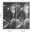 |
Fig. 2. Simulated images of Hα at nominal line center, Δλ = 0 Å, from the model atmosphere in vertically emergent intensity. The images are given in brightness temperature Tb and are clipped at 2.8 and 8.5 kK. Panel a: 1.5D radiative transfer where each column in the snapshot is treated as a plane-parallel atmosphere. Panel b: full 3D radiative transfer. The minimum, maximum, and average Tb for the entire field of view (FOV) is provided in a label above each panel. |
The brightest features have a similar morphology in the 1D and 3D computations. Analysis shows that this is caused by the high mass density, and thus strong collisional coupling of the source function to the temperature in the chromosphere at these locations (see Sect. 4.6.1). Therefore, this can potentially open the possibility of including Hα in inversions that assume 1D geometry (Milić & van Noort 2018; de la Cruz Rodríguez et al. 2019) in active regions.
3. Observations
We used two different observational datasets to compare with the synthetic data. The first dataset is an observation of active region NOAA 12593, located near the disk center at θx = −68″ and θy = −6″ (helioprojective-Cartesian coordinates), taken at the SST (Scharmer et al. 2003) on September 19, 2016, at 09:31–09:57 UT.
The data were recorded simultaneously by the CHROMIS and CRisp Imag- ing SpectroPolarimeter (CRISP; Scharmer et al. 2008) instruments, which observed Fe I 6301 Å, Fe I 6032 Å, Hα, Ca II 8542 Å, and Ca II K. We only used the latter three spectral lines. The data were processed with the CRISPRED and CHROMISRED pipelines (de la Cruz Rodríguez et al. 2015; Löfdahl et al. 2018). A more detailed description of the SST observation are provide in Leenaarts et al. (2018); it suffices to mention for this work that we obtained near-simultaneous spectral scans in all three lines.
Unfortunately, there is no co-observation with the Interface Region Imaging Spectrograph (IRIS; De Pontieu et al. 2014). Therefore, we used IRIS data observed on February 5, 2016, at 08:21–09:12 UT to be able to compare our computations of the Mg II k line. The IRIS target is an emerging active region NOAA 12494, observed near the disk center at θx = −96″ and θy = −98″.
Figure 3 shows the line core images for all four spectral lines. Panels a-c show an active region covered with fibrils and a sunspot in the top right corner. Panel d shows a slit jaw image at the nominal line center of Mg II k, of an active region with one sunspot located on the left side and a sunspot outside the FOV on the right side. Long elongated fibrils are connected with the sunspots and pores located in the middle of the FOV.
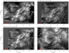 |
Fig. 3. Observations of two active regions close to the disk center at the nominal line center of (a) Ca II K (SST/CHROMIS), (b) Hα (SST/CRISP), (c) Ca II 8542 Å (SST/CRISP), and (d) Mg II k (IRIS). Panels a–c: NOAA 12593. Panel d: NOAA 12494. The images are given in brightness temperature Tb and are clipped at 4.5–6 K for Ca II K, 3.9–6 Kk for Hα, 3.8–6 kK for 8542 Å, and 4.7–7 kK for Mg II k. Above the top left corner of each panel we show the minimum, maximum, and average brightness temperature for the FOV. Panels a–c have the same coordinate scale, while panel d has a different scale. |
4. Results
4.1. Effect of non-LTE electron density on the emergent intensity
We compared how different are electron densities computed either using the LTE EOS for all chemical species or by treating hydrogen in non-LTE with imposed conservation of charge. We found severe differences between the LTE and non-LTE values in the middle and upper chromosphere.
On average the inclusion of charge conservation in the calculations leads to higher electron densities compared to LTE in cold areas of the chromosphere, owing to an increased hydrogen ionization degree through the Balmer continuum. This difference was largest (by a factor ∼103) in cold pockets (3250 K) right below the transition region. In hot areas in the mid-chromosphere we typically find a somewhat lower electron density than in LTE.
Figure 4 illustrates how the non-LTE electron densities change the emergent intensity in Mg II k. For the spatially averaged intensity, the maximum relative difference reaches 30% near the line core (Fig. 4a). Individual profiles show even larger differences depending on which chromospheric structure they are emerging from. In dark fibrils the non-LTE intensity drops below the LTE intensity (Fig. 4b), but in flare ribbons it increases significantly near the line core (Fig. 4c). Therefore, in the rest of the paper we only present results using the non-LTE electron density.
 |
Fig. 4. Dependence of the vertically emergent intensity in Mg II k on how the electron density is computed. Panel a: spatially averaged relative change in the intensity, which is computed using either non-LTE or LTE electron densities. Panels b,c: line intensities expressed as brightness temperature Tb and computed using LTE (blue) or non-LTE (red) electron density at two structures indicated in Fig. 7. Panel b: dark fibril, red dot in Fig. 7. Panel c: flare ribbon, blue dot in Fig. 7. |
4.2. Formation heights
Calcium and magnesium are both predominantly singly ionized in the chromosphere. Mg II ionizes to Mg III at slightly higher temperatures owing to the higher ionization potential of Mg II (15.0 eV) compared to Ca II (11.87 eV). Both the Mg II h&k and Ca II H&K lines have the ground state as their lower level, so their opacity scales approximately with the density as long as Mg II and Ca II are the dominant ionization stage. As Mg II is 18 times more abundant than Ca II, the line cores of Mg II h&k are formed a few scale heights higher up in the chromosphere than the line cores of Ca II H&K (Leenaarts et al. 2013a; Bjørgen et al. 2018).
In contrast, the lower level of Hα is an excited state at 10.2 eV above the ground state. In LTE this makes the line opacity very sensitive to the temperature. In the solar chromosphere, the Hα line opacity depends in a complicated way on the temperature, density, and the time history of the atmosphere owing to the nonequilibrium ionization of hydrogen. Leenaarts et al. (2012) investigated the formation of Hα in a radiation-MHD simulation of the quiet Sun and found that in those circumstances the line can be reasonably accurately modeled assuming statistical equilibrium. In that simulation they also found that the line opacity weakly depended on temperature and mainly depended on mass density. Carlsson & Leenaarts (2012) investigated the ionization of H I, Ca II, and Mg II and found that at temperatures above 15 kK, the fraction of H I is much higher than the fractions of Ca II and Mg II. Rutten & Rouppe van der Voort (2017) and Rutten (2017) argued similarly, albeit based on LTE, that Hα can have an appreciable opacity at temperatures well above 20 kK.
Studies of the formation heights of the line cores based on the quiet-Sun-like simulation of Carlsson et al. (2016) indicate that Hα forms 300–1000 km below Ca II K and Mg II k (Leenaarts et al. 2013a). The similarity of the line-core images in Fig. 3a,b casts doubt on the validity of this result in active regions. We therefore investigated the formation heights in the MURaM simulation.
We measured the formation heights at optical depth unity in the corresponding line cores of Hα, Mg II k, Ca II K, and Ca II 8542 Å. Figure 5 shows differences between the formation height of Hα and the formation heights of the rest of the lines. On average, the core of Hα, k3, and K3 features are formed at similar heights and roughly 150 km above the core of 8542 Å throughout the FOV.
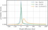 |
Fig. 5. Distribution of the differences between the line-core formation heights of Hα and, respectively, Mg II k (blue), Ca II K (green), and Ca II 8 542 Å (orange). |
We note that the distributions have long tails toward positive values meaning that Hα can be formed much higher than the other lines. These points, where the height difference exceeds 1000 km, constitute for the FOV ∼2% for both Mg II k and Ca II K and ∼5% for 8542 Å. Figure 6 illustrates this case. At 3.22 Mm where the Hα core reaches optical depth unity, H I is only 97.5% ionized and at the same location the metals (Ca II and Mg II) are 99.9% ionized. Hα is formed highest in the atmosphere. It retains opacity where the lines from the metals have none because H I does not ionize as quickly as Ca II and Mg II when the temperature increases.
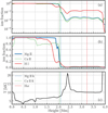 |
Fig. 6. Fraction of an element in a given ionization state for Mg II (blue solid), Ca II (green solid), and H I (red solid) in a column of the MURaM model atmosphere. Panel a: log-scaled ionization fractions. Panel b: linearly scaled ionization fractions. Panel c: gas temperature (black solid) as a function of height. Vertical lines show the maximum formation heights of Mg II k (dashed blue), Ca II K (dashed green), and Hα (dashed red). |
4.3. Synthetic images
In Fig. 7 we show the vertically emergent intensity in the line core of Ca II 8542 Å, Ca II K, Mg II k, and Hα. We first describe what we see at nominal line center (Fig. 7, top panels). In all four spectral lines we see large elongated structures emanating from the two sunspots (see Fig. 1b), similar to large-scale fibrils seen in observations. From now on we call the structures on our synthetic images fibrils as well. The fibrils are much more pronounced in Hα than in the other lines. The longest fibrils extend up to 35 Mm.
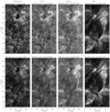 |
Fig. 7. Simulated images of Ca II 8542 Å, Ca II K, Mg II k, and Hα from the model atmosphere in vertically emergent intensity. Top row: at nominal line center, Δλ = 0 Å. Bottom row: at wavelengths corresponding to the maximum formation height, maxz(τ = 1). Intensity is expressed as brightness temperature Tb and is clipped to same ranges in each column: 3.6–7 kK for Ca II 8 542 Å, 3.6–7 kK for Ca II K, 3.6–8 kK for Mg II k, and 3.6–10 kK for Hα. The minimum, maximum, and average Tb for the entire FOV is provided in a label above each panel. Colored symbols indicate the following structures: a dark fibril (red dot) and a flare ribbon (blue dot), see Fig. 4; an active region in emission (orange cross), see Fig. 12; an active region in emission with a strong velocity gradient (blue cross), see Fig. 13; a sunspot (green cross), see Fig. 14; a fibril (red cross), see Fig. 15. |
A careful comparison of the panels reveals that the fibrils appear somewhat different in Ca II 8542 Å, looking translucent with the background chromosphere shining through. This is especially visible in the top right corner. This is consistent with the lower formation height of this line, as discussed in Sect. 4.2.
In Hα, we observe several very bright patches close to the sunspots, which connect with a thinner bright arc. These patches look similar to flare ribbons. Along these ribbons the Hα profiles are in emission and very broad. In Ca II K and Mg II k we see only a weak signature of the ribbon, while in Ca II 8542 Å it is only visible as a small brightness enhancement to the right of the upper sunspot.
Now we describe what we see at wavelengths where the intensity in each pixel individually is taken at the wavelength where the formation height is largest. (Fig. 7, bottom panels). These images thus compensate for Doppler shifts of the line core (Leenaarts et al. 2013a; Bjørgen et al. 2018).
The Hα image is relatively unchanged, while the other images are more affected. This difference is caused by the large thermal broadening of Hα compared to the other lines, which makes it less sensitive to Doppler motions. In the Ca II and Mg II lines the carpet of fibrils now appears thicker and sharper than in the nominal line-core images. The flare ribbons are now visible in these lines, even in Ca II 8542 Å.
The simulated images exhibit features that somewhat resemble observational features in our Fig. 3 or Fig. 1 by Reardon et al. (2011). The observations show that Ca II K and Hα trace roughly the same structures. The Ca II 8542 Å often shows different fibrils with more visible patterns of waves and shocks from the lower chromosphere.
The SST/CRISP, SST/CROMIS, and, to a lesser extent, IRIS observations show finer structures than the synthetic images. This is most likely caused by the finite horizontal grid spacing (96 km) of the model atmosphere compared to the resolution of the observations (∼100 km for SST, ∼250 km for IRIS). Bjørgen et al. (2018) showed for radiation-MHD models of the enhanced network that synthetic fibrils get thinner and closer in appearance to the observed fibrils if the horizontal grid spacing of the simulation decreases from 48 km to 31 km.
Leenaarts et al. (2012, 2013a) and Bjørgen et al. (2018) computed synthetic images of the chromosphere in Hα, Ca II K, and Mg II k from the quiet Sun simulation by Carlsson et al. (2016). Their line-core images showed ordered fibrils stretching between two opposite magnetic polarities separated by about 8 Mm, which also limited the fibril length to 8 Mm. Hansteen et al. (2017) computed Hα and Mg II h for a flux emergence simulation that was also computed with the Bifrost code. Their Hα line-core image showed some thick unordered fibrils with a maximum length of 12 Mm, while the corresponding Mg II h image does not show a clear fibril structure.
The current MURaM simulation is the first simulation including a chromosphere that contains the spatial scales of an entire active region, and succeeds in reproducing long fibrils connecting the opposite polarities of an active region as seen in observations. In the following subsection we analyze some of the structures seen in the synthetic intensity images in more detail.
4.4. Synthetic fibrils
The horizontal domain size of the current MURaM simulation is 98 Mm × 49 Mm. This large size allows for ∼40 Mm long magnetic loops in the chromosphere that connect the two sunspots. The synthetic images in Fig. 7 show long fibrils that follow the large-scale structure of the field. We investigated whether the fibrils trace the magnetic field, i.e., both the vertical and horizontal components.
Figure 8 shows the line-core intensity of Hα, with the horizontal component of the magnetic field at the formation height overplotted. The fibrils follow the horizontal magnetic field direction in most places, but at some locations (such as the arrow at (X, Y) = (54, 34) Mm) they do not.
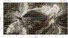 |
Fig. 8. Image of Hα at nominal line center overplotted with the horizontal magnetic field directions (orange arrows) at the formation height. The arrows are plotted every 30th grid point. The visibility of Hα fibrils is artificially enhanced using unsharp masking. The blue and red lines indicate two slices along selected fibrils illustrated in Figs. 9 (blue) and 10 (blue and red). |
Figure 9 illustrates the magnetic field component in the plane of a model atmosphere slice that follows the blue line in Fig. 8. As expected for active regions, the magnetic pressure exceeds the gas pressure at low heights in the atmosphere, as illustrated by the plasma β = 1 = Pgas/PB curve, which goes from −1 Mm to 0.5 Mm. The lowest height of β = 1 curve is located at the sunspot (X > 69 Mm), where the magnetic field strength reaches 6 kG in the photosphere. Horizontally the fibril spans from X = 51 Mm to X = 68 Mm and for X < 51 Mm the cut intersects an area of the atmosphere that shows irregular short structures in the Hα image of Fig. 8.
 |
Fig. 9. Mass density in a vertical cut through the model atmosphere along the blue line in Fig. 8. For each spectral line mentioned in the legend, corresponding dashed curves show the maximum formation height at optical depth unity. The white dotted line shows the first occurrence from the upper convection zone where the magnetic pressure equals gas pressure (β = 1). The arrows show the direction of the magnetic field vector in the plane of the cut along the formation height curve of Hα. These arrows are plotted every tenth grid point. |
In the sunspot, the transition region is very low, 1 Mm above the quiet photosphere and roughly 2 Mm above the local height of continuum optical depth unity. so that all four spectral lines are formed mostly at the same height. The angle between the field vector and the τ = 1 surface is large. In the area where x < 51 Mm we see intrusions of high mass density sticking into the low-density corona, and the τ = 1 surface follows these mass intrusions. We speculate that these could be Type I spicules as simulated before in 2D (e.g., Hansteen et al. 2006), but this is impossible to confirm without analyzing a time series.
Now we turn our attention to the long loop-like structure between X = 51 Mm and X = 68 Mm in Fig. 9. The magnetic field vector and the τ = 1 height curve of Hα are parallel to each other for a large fraction of the loop. It is not shown in the figure, but this is true to a lesser extent for the other lines, which all exhibit jumps in their formation height. We analyzed a number of other fibrils not illustrated in this work and found that for clearly defined fibrils, Hα indeed tends to follow the magnetic field lines. This is in contrast with the results from Leenaarts et al. (2015), who found in a simulation of quiet sun fibrils that Hα fibrils typically follow the horizontal component, but not the vertical component, of the magnetic field.
To investigate the magnetic field we traced two fibrils to get a more detailed overview. They are indicated by blue and red curves in Fig. 8. Figure 10 shows the offset between the inclination of the τ = 1 curve and magnetic field vector, and the offset between the azimuths of the fibril and magnetic field. We only show results for Hα and Ca II 8542 Å, as they are the lines with the highest and lowest formation heights.
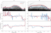 |
Fig. 10. Alignment between the magnetic field vector and the curve of the maximum formation height at optical depth unity in two selected vertical slices. Left column: blue curve fibril in Fig. 8. Right column: red curve fibril in Fig. 8. Top row: formation heights of Hα (red) and Ca II 8542 Å (blue) with the β = 1 height (white dotted) layered over the mass density (grayscale background). Middle row: angle between the inclination of the magnetic field and the τ = 1 curve. Bottom row: angle between the magnetic field azimuth and the azimuth of the fibril. |
Figure 10a shows the same fibril as in Fig. 9 in between 51 Mm and 68 Mm. The inclination offset is around 10° for both lines. However, the formation height curve of Hα is more smooth, while the Ca II 8542 Å curve has a number of sudden jumps, which cause spikes in the offset curve. Physically, these jumps mean that depending on where you look along the fibril, you see different field lines, but locally the formation height curve follows the magnetic field inclination. The Hα fibril follows the azimuth very well, while the Ca II 8542 Å shows offsets up to 10°.
Figure 10b shows the offsets of a curved fibril indicated with a red line in Fig. 8. We see almost the same behavior as the previous fibril shows: in Hα this fibril follows both the inclination and the azimuth of the magnetic field vector very well, while in Ca II 8542 Å it follows these less so owing to large changes in the formation height.
In addition to the fibrils analyzed in this work we manually investigated a number of other fibrils, which show similar behaviors. We thus conclude that most fibrils in this active region simulation do trace the horizontal magnetic field, especially for spectral lines formed in the upper chromosphere (Ca II H&K, Mg II h&k, and Hα). Fibrils seen in 8 542 Å mostly, but not always, trace the horizontal component of the magnetic field. This agrees with the observational studies (de la Cruz Rodríguez & Socas-Navarro 2011; Asensio Ramos et al. 2017). We note that this simulation does not include ambipolar diffusion. Inclusion of this process allows the magnetic field to be less aligned with density and temperature structures in the chromosphere because it relaxes the frozen-in condition (Martínez-Sykora et al. 2016). However, simulations with ambipolar diffusion have only been performed in 2.5D simulations (Cheung & Cameron 2012) or simplified 3D simulations (Arber et al. 2007) or radiative 3D simulation with only photosphere (Danilovic 2017). Therefore, only a full 3D MHD simulation that includes chromosphere with ambipolar diffusion should be used to investigate the possible misalignment properly (see also Sect. 3.8.3 of Cheung & Isobe 2014).
4.5. Spatially averaged spectral profiles
We compared the spatially averaged synthetic spectra with observations from SST and IRIS to see how far the model is from the real Sun. Although the solar features represented in the observed and simulated samples are quite different, the comparison also allows us to place this model in the context of previous studies (e.g., Leenaarts et al. 2013a; Bjørgen et al. 2018). Figure 11 shows the spatially averaged profiles of Ca II 8542 Å, Ca II K, Mg II k, and Hα from the model atmosphere and observations (see Sect. 3). Two different averages are shown for the synthetic spectra: the entire model atmosphere (panels a–d), and in a patch with relatively weak magnetic field (panels e–h). We note that the observations are not in any way chosen to represent all active regions, they just illustrate how average line profiles in active regions look.
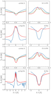 |
Fig. 11. Spatially averaged line profiles of Ca II 8542 Å, Ca II K, Mg II k, and Hα expressed as brightness temperature Tb for the model atmosphere and our observations. Blue: observations; red: model atmosphere at full resolution; green dashed: model atmosphere spectrally degraded to match the resolution of the observations. Panels a–d: spatial averages for the entire model FOV. Panels e–h: spatial averages for a weakly magnetized patch only. The Hα and Mg II k lines are not degraded spectrally. |
The observations of Hα and Ca II 8542 Å show absorption profiles, while Mg II k and Ca II K show a double-peaked central reversal (marginally visible in Ca II K owing to the spectral resolution of SST/CHROMIS). The synthetic spectra for the atmosphere outside the flare ribbons show qualitatively the same behavior, but substantial differences in a quantitative sense.
The averaged spectra from the model atmosphere gives a peak separation of 16 km s−1 (0.15 Å) for Mg II k and 10.5 km s−1 (0.14 Å) for Ca II K. These numbers are ∼30% larger than those reported for Bifrost simulations of the quiet Sun (Leenaarts et al. 2013a; Bjørgen et al. 2018), but still ∼1.5–2 times smaller than observed for the quiet Sun.
The averaged profiles of Ca II K and 8542 Å show that the model atmosphere is colder in the lower chromosphere and photosphere than the observations. The synthetic line wings of Mg II k have a higher intensity than the observations. We also note that the inner wings of the Ca II 8542 Å, Ca II K, and Hα line lie below the observed intensity, while the Mg II k wings lie above it.
Inspection of Fig. 11d shows that the averaged Hα profile has a central emission and a weak and blueshifted central absorption core, in stark contrast to the observations. Figure 11h shows that the core behaves as usual in the less magnetized patch of the simulation. We show in Sect. 4.6.1 that the filling of the Hα core in the averaged profile is caused by a strong Hα emission in the flare ribbons.
4.6. Spatially resolved synthetic profiles
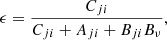
In Figs. 12–15 we explain the formation of line intensity profiles in three different structures in the simulation: flare ribbons (with and without strong velocity gradients), a fibril, and a sunspot umbra. The top row of each figure shows the profiles for each line; the bottom row shows the temperature and line source functions for Hα and Ca II 8542 Å in the left panel, the two-level photon destruction probability in the middle panel, and the height where τν = 1 for each line together with the vertical velocity in the right panel. The photon destruction probability is defined as
 (1)
(1)
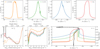 |
Fig. 12. Line formation in a flare ribbon (orange cross in Fig. 6). Top row: profiles of vertically emergent intensity, expressed as brightness temperature Tb, as function of frequency from line center (in Doppler shift units) for Ca II 8542 Å (orange), Ca II K (green), Mg II k (blue), and Hα (red). Bottom left: line source functions for Hα (red dashed) and Ca II 8542 Å (orange dashed), expressed as excitation temperature, and the gas temperature (solid black) as a function of column mass. Bottom middle: photon destruction probabilities for each of the lines. Bottom right: height of optical depth unity (solid colored) and the vertical velocity (solid black dots indicate the grid points, upflow is positive) as a function of frequency from line center in Doppler shift units. |
 |
Fig. 13. Line formation in a flare ribbon with strong velocity gradient (blue cross in Fig. 6). The figure follows the same format as Fig. 12. |
 |
Fig. 14. Line formation in a sunspot (green cross in Fig. 6). The figure follows the same format as Fig. 12. |
 |
Fig. 15. Line formation in a fibril (red cross in Fig. 6). The figure follows the same format as Fig. 12. |
with the downward collisional rate Cji, the Einstein coefficients Aji for spontaneous de-excitation, Bji for induced de-exitation, and the Planck function Bν. We do not show the line source functions for Ca II K and Mg II k because they are frequency-dependent owing to PRD effects. We show ϵ because it gives an indication of the sensitivity of the line source function to the local temperature using the two-level source function approximation,  .
.
4.6.1. Flare ribbons
We investigated our model atmosphere and line formation in the flare ribbons, which are shown in two columns in Figs. 12 and 13. The top panels of Fig. 12 show an example of broad, slightly redshifted emission peaks in all four lines. The chromosphere has a high mass density as evidenced by the high values of ϵ (which is roughly proportional to the electron density). The transition region lies at a high column mass of 10−4.2 g cm−2, and the chromospheric temperature rise starts deep in the atmosphere at 0.2 g cm−2. This partly explains why the ribbons look so similar when the intensities are computed in 1D and 3D (see Fig. 2). The strong chromospheric temperature rise leads to a source function increasing with height for all lines, leading to the emission profiles, while the deep location of the onset of the rise causes the wide symmetric base of the emission peaks, especially for Mg II k. The downflow just below the transition region causes the redshift of the emission peak.
These relatively smooth flare ribbon profiles are actually rather rare in our FOV. We often find more complex spectral profiles, such as shown in Fig. 13. These profiles typically show multiple-peaked profiles in Ca II K and Mg II k and have strongly Doppler-shifted emission peaks. The Hα profile is very broad and has its strongest emission peak blueshifted by 130 km s−1. The temperature in the chromosphere shows multiple peaks with low temperatures between the peaks. The mass density, and thus the photon destruction probability, are again high and the transition region is again located at a high column mass. The atmosphere differs from that shown in Fig. 12 in that the transition region harbors a strong velocity gradient. The cores of Mg II k and Ca II K form completely in the chromosphere in this gradient. The strongest emission peak in Hα reaches optical depth unity between the last chromospheric grid point with a temperature of 5.5 kK and the first transition-region/coronal grid point, which has a temperature of 450 kK, i.e., in the temperature gradient indicated by the nearly vertical black line in the lower left panel of Fig. 13.
The finite vertical resolution of the model atmosphere produces the peculiar, multiple-peaked line shapes of Mg II k, and Ca II K. The difference in vertical velocity between adjacent grid points is larger than the Doppler width and this causes spurious emission peaks, as explained by Ibgui et al. (2013). This is reflected in the peaks in the z(τν = 1) curves in the lower right panel. The formation height is large at the velocities of the grid points (black filled circles), but drops to low values when more than a Doppler width away from the velocities at the grid points.
The multiple emission peaks are thus artifacts produced by the limited spatial resolution in the radiative transfer computation. Had the velocity gradient been properly resolved, then these line profiles would show a broad asymmetric emission peak.
The Hα profile does not show such strong emission peaks. The emission peak at Δv = −120 km s−1 is, however, badly resolved. The frequency grid is not fine enough to resolve the right flank, and as stated before, the peak forms within a single grid interval, which constitutes the interface between the chromosphere and transition region; we compare the brightness temperature of the emission peak of 13 kK to the source function in the lower right panel. In this interval the optical depth increases from 10−5 to 1.2. The contribution function is thus not properly resolved and the resulting intensity depends on the chosen solution scheme. We investigated the source function and exactly in this grid interval its changes from two-level behavior in the chromosphere to recombination-radiation-dominated in the transition region.
4.6.2. Sunspot
Figure 14 shows the line formation in a sunspot in the model atmosphere. The Hα core is in emission, and the three other spectral lines show double-peaked profiles. This is common in the model atmosphere; we find only a few locations where Hα is in absorption and the other lines have single emission peaks.
The temperature stratification as shown in Fig. 14 is common across the sunspots, from the temperature minimum the gas temperature monotonically increases toward the transition region. The Hα line is in emission because the line core is formed in the steep temperature gradient of the transition region with a high source function. The line cores of the other lines tend to be formed just below the transition region. The chromosphere has a temperature rise that is deep enough to cause emission peaks.
Compared with many available observations (e.g., Panos et al. 2018; Maurya et al. 2013; de la Cruz Rodríguez et al. 2013; Felipe et al. 2011; Engvold 1967), we see that the simulated sunspot profiles are somewhat unusual: observed Hα profiles are typically in absorption; the Ca II K and Mg II k profiles are typically, but not always, single peaked; and Ca II 8542 Å is in absorption and only shows emission when an umbral flash passes through.
4.6.3. Fibril
Figure 15 shows the typical line formation in a fibril. In this case Hα is in absorption, Ca II K, Mg II k, and Ca II 8542 Å each have an asymmetric double-peaked emission core. We find that this situation is common for Hα, Ca II K, and Mg II k. The density in the chromosphere is relatively low, and ϵ is an order of magnitude smaller than in the flare-ribbon columns. The Hα line core is formed below the transition region and therefore is not influenced by the increase in the source function there.
The Ca II 8542 Å line shows much more variation, ranging from pure absorption to wide and asymmetric profiles with three emission peaks. The line is mainly in absorption in fibrils in our data, while we also find some instances of profiles with a double-peaked central reversal as in Fig. 15.
5. Discussion and conclusions
Cheung et al. (2018) performed a radiation-MHD simulation of an active region including emergence of a new flux that produced a flare-like reconnection event in the corona. We took a snapshot from a rerun of their simulation with twice the original numerical resolution.
This numerical experiment, aimed only at investigating the corona, produced a unique dataset suitable for investigating the chromosphere as well. The simulation domain is geometrically 4 × 2 × 3 times bigger and models a much more active chromosphere than the commonly used, publicly available Bifrost simulation (Carlsson et al. 2016).
The trade-off for getting the large domain size is that the grid spacing, 96 km horizontally and 32 km vertically, is relatively coarse. Radiative energy losses in the photosphere and corona are approximated using the gray LTE transfer. The absorption of coronal radiation in the chromosphere is not included. The EOS assumes LTE, whereas hydrogen and helium both require nonequilibrium ionization (Leenaarts et al. 2007; Golding et al. 2014). There are no interactions between ions and neutral species, which significantly structure and heat the chromosphere (Martínez-Sykora et al. 2012, 2017). These simplifications have an impact on the structure of the chromosphere, both for the temperature and density in the model atmosphere. However, these simplifications do not affect the large-scale magnetic structure in the chromosphere. They do not distort the formation of flare ribbons, chromospheric evaporations through heat conduction either, even though the exact location of the transition region changes if more accurate radiative losses are included.
In this paper we took one snapshot of this MURaM simulation and solved numerically the problem of 3D radiative transfer for H I, Ca II, and Mg II in non-LTE including PRD in the Mg II k and Ca II K lines. We corrected the electron density by treating hydrogen in statistical equilibrium together with an equation for charge conservations. On the radiative transfer side, this is a large improvement over the electron density evaluated in LTE. For the sake of numerical stability and computational speed, we set the minimum temperature in the model atmosphere to 3250 K, we used a simple approximation for the pressure broadening of Hα, and we limited the size of our H I model atom.
The finite grid spacing resulted in a poor sampling in both frequency and optical depth that led to artifacts in the line profiles when the line-forming region contains large gradients in temperature, velocity and/or density. While these minor weaknesses should be addressed in future work to allow detailed quantitative comparison with observations, they have no consequences for the qualitative results shown this paper.
We showed that 3D non-LTE radiative transfer computations including charge conservation and PRD can handle a large variation in all physical quantities, in a different parameter regime (active region) than studied before (more quiet-sun-like; Carlsson et al. 2016).
The synthetic line-core images have shown long (∼35 Mm) strands connecting the opposite-polarity sunspots, that resemble fibrils seen in observations. We established that the strong fibrils seen in Hα are mostly aligned with the magnetic field direction. Fibrils seen in the other lines are less aligned, especially those in Ca II 8 542 Å, which suffer from sudden changes of the height of optical depth unity. This contrasts with the findings in Leenaarts et al. (2015), who found that in more quiet-Sun circumstances only a fraction of the fibrils seen in Hα follow the same field line.
In 3D MHD simulations of quiet Sun, Leenaarts et al. (2012, 2013a) found that the cores of Mg II k and Ca II are both formed in the upper chromosphere in a wide range of heights following the transition region, while the cores of Hα and Ca II 8542 Å are formed at lower heights in the middle chromosphere.
We have found two important differences with this in the MURaM simulation. Firstly, the Hα line is formed in a much larger range of heights. Secondly, the cores of Hα, Mg II k, and Ca II K are formed at very similar heights while the core of Ca II 8542 Å is formed only some 150 km below them. This qualitatively agrees with observations of active regions, which show a very similar appearance in the cores of Hα and Ca II K (Leenaarts et al. 2018). Given that the model used in this paper manages to reproduce the overall appearance in all chromospheric observables we synthesized, this indicates that the model gives a decent representation of long solar fibrils.
The flare ribbons in this simulation are caused by thermal conduction only. They appear bright in the line cores because the thermal conduction and dense coronal loops above the ribbon cause a hot and dense upper chromosphere, and there is sufficient electron density to couple the source function to the local temperature. This mechanism is similar to what Carlsson et al. (2015) proposed for Mg II k in plages. We find synthetic line profiles that are broad, asymmetric, and have a single emission peak similar to the profiles observed in flare ribbons.
The flare ribbons are poorly visible in Ca II 8542 Å, in contrast to observations (e.g., Kleint 2012). This agrees with the standard flare model that requires beams of nonthermal electrons or Alfvénic waves to deposit thermal energy in the middle chromosphere. Nevertheless, the visibility of the flare ribbons hints that the fraction of the flare energy transported down by thermal conduction is enough to significantly alter the structure of the chromosphere.
This study is just a first step toward understanding the chromosphere in active regions using 3D radiation-MHD simulations. In our study, we only touched on the formation of the strongest chromospheric lines. Future studies should look into the formation of the lines in more detail.
MPS/University of Chicago Radiative MHD.
Acknowledgments
The Swedish 1-m Solar Telescope is operated on the island of La Palma by the Institute for Solar Physics of Stockholm University in the Spanish Observatorio del Roque de los Muchachos of the Instituto de Astrofísica de Canarias. The computations were performed on resources provided by the Swedish National Infrastructure for Computing (SNIC) at the High Performance Computing Center North at Umeå University and the PDC Centre for High Performance Computing (PDC-HPC) at the Royal Institute of Technology in Stockholm. J. L. was supported by a grant (2016.0019) of the Knut och Alice Wallenberg foundation. SD and JdlCR were supported by a grant from the Swedish Civil Contingencies Agency (MSB). This study has been discussed within the activities of team 399 “Studying magnetic-field-regulated heating in the solar chromosphere” at the International Space Science Institute (ISSI) in Switzerland. JdlCR is supported by grants from the Swedish Research Council (2015-03994), the Swedish National Space Board (128/15). This project has received funding from the European Research Council (ERC) under the European Union’s Horizon 2020 research and innovation programme (SUNMAG, grant agreement 759548). AVS acknowledges financial support from the Spanish Ministry of Economy and Competitiveness (MINECO) under the 2015 Severo Ochoa Program MINECO SEV-2015-0548. The National Center for Atmospheric Research is sponsored by the National Science Foundation. We would like to thank Adam F. Kowalski and Joel C. Allred for providing us their modified RH code, which includes the unified theory of electric pressure broadening. J. P. B. would thank Gregal J. M. Vissers for the help in calibrating the IRIS data, and Carolina Robustini for discussions.
References
- Allred, J. C., Hawley, S. L., Abbett, W. P., & Carlsson, M. 2005, ApJ, 630, 573 [NASA ADS] [CrossRef] [Google Scholar]
- Arber, T. D., Haynes, M., & Leake, J. E. 2007, ApJ, 666, 541 [NASA ADS] [CrossRef] [Google Scholar]
- Aschwanden, M. J., Reardon, K., & Jess, D. B. 2016, ApJ, 826, 61 [CrossRef] [Google Scholar]
- Asensio Ramos, A., de la Cruz Rodríguez, J., Martínez González, M. J., & Socas-Navarro, H. 2017, A&A, 599, A133 [NASA ADS] [CrossRef] [EDP Sciences] [Google Scholar]
- Beckers, J. M. 1964, PhD Thesis, Sacramento Peak Observatory, Air Force Cambridge Research Laboratories, MA, USA [Google Scholar]
- Benz, A. O. 2008, Liv. Rev. Sol. Phys., 5, 1 [Google Scholar]
- Bjørgen, J. P., Sukhorukov, A. V., Leenaarts, J., et al. 2018, A&A, 611, A62 [NASA ADS] [CrossRef] [EDP Sciences] [Google Scholar]
- Carlson, B. G. 1963, in Methods in Computational Physics, Vol. 1, Statistical Physics, Methods in Computational Physics: Advances in Research and Applications, eds. B. Alder, S. Fernbach, & M. Rotenberg (New York, NY, USA: Academic Press), 1 [Google Scholar]
- Carlsson, M., & Leenaarts, J. 2012, A&A, 539, A39 [NASA ADS] [CrossRef] [EDP Sciences] [Google Scholar]
- Carlsson, M., Leenaarts, J., & De Pontieu, B. 2015, ApJ, 809, L30 [NASA ADS] [CrossRef] [Google Scholar]
- Carlsson, M., & Stein, R. F. 1992, ApJ, 397, L59 [NASA ADS] [CrossRef] [Google Scholar]
- Carlsson, M., & Stein, R. F. 2002, ApJ, 572, 626 [NASA ADS] [CrossRef] [Google Scholar]
- Carlsson, M., Hansteen, V. H., Gudiksen, B. V., Leenaarts, J., & De Pontieu, B. 2016, A&A, 585, A4 [NASA ADS] [CrossRef] [EDP Sciences] [Google Scholar]
- Cheung, M. C. M., & Cameron, R. H. 2012, ApJ, 750, 6 [NASA ADS] [CrossRef] [Google Scholar]
- Cheung, M. C. M., & Isobe, H. 2014, Liv. Rev. Sol. Phys., 11, 3 [Google Scholar]
- Cheung, M. C. M., Rempel, M., Chintzoglou, G., et al. 2018, Nat. Astron., 173 [Google Scholar]
- Danilovic, S. 2017, A&A, 601, A122 [NASA ADS] [CrossRef] [EDP Sciences] [Google Scholar]
- de la Cruz Rodríguez, J., & Socas-Navarro, H. 2011, A&A, 527, L8 [NASA ADS] [CrossRef] [EDP Sciences] [Google Scholar]
- de la Cruz Rodríguez, J., Rouppe van der Voort, L., Socas-Navarro, H., & van Noort, M. 2013, A&A, 556, A115 [NASA ADS] [CrossRef] [EDP Sciences] [Google Scholar]
- de la Cruz Rodríguez, J., Löfdahl, M. G., Sütterlin, P., Hillberg, T., & Rouppe van der Voort, L. 2015, A&A, 573, A40 [NASA ADS] [CrossRef] [EDP Sciences] [Google Scholar]
- de la Cruz Rodríguez, J., Leenaarts, J., Danilovic, S., & Uitenbroek, H. 2019, A&A, 623, A74 [NASA ADS] [CrossRef] [EDP Sciences] [Google Scholar]
- De Pontieu, B., Title, A. M., Lemen, J. R., et al. 2014, Sol. Phys., 289, 2733 [NASA ADS] [CrossRef] [Google Scholar]
- Engvold, O. 1967, Sol. Phys., 2, 234 [CrossRef] [Google Scholar]
- Felipe, T., Khomenko, E., Collados, M., & Beck, C. 2011, J. Phys.: Conf. Ser., 271, 012040 [CrossRef] [Google Scholar]
- Fletcher, L., Dennis, B. R., Hudson, H. S., et al. 2011, Space Sci. Rev, 159, 19 [Google Scholar]
- Fontenla, J. M., Avrett, E. H., & Loeser, R. 1993, ApJ, 406, 319 [NASA ADS] [CrossRef] [Google Scholar]
- Golding, T. P., Carlsson, M., & Leenaarts, J. 2014, ApJ, 784, 30 [NASA ADS] [CrossRef] [Google Scholar]
- Golding, T. P., Leenaarts, J., & Carlsson, M. 2016, ApJ, 817, 125 [NASA ADS] [CrossRef] [Google Scholar]
- Gudiksen, B. V., Carlsson, M., Hansteen, V. H., et al. 2011, A&A, 531, A154 [NASA ADS] [CrossRef] [EDP Sciences] [Google Scholar]
- Hansteen, V. H., Archontis, V., Pereira, T. M. D., et al. 2017, ApJ, 839, 22 [NASA ADS] [CrossRef] [Google Scholar]
- Hansteen, V. H., De Pontieu, B., Rouppe van der Voort, L., van Noort, M., & Carlsson, M. 2006, ApJ, 647, L73 [NASA ADS] [CrossRef] [Google Scholar]
- Heinzel, P. 1995, A&A, 299, 563 [NASA ADS] [Google Scholar]
- Ibgui, L., Hubený, I., Lanz, T., & Stehlé, C. 2013, A&A, 549, A126 [NASA ADS] [CrossRef] [EDP Sciences] [Google Scholar]
- Judge, P. G., Tritschler, A., & Chye Low, B. 2011, ApJ, 730, L4 [NASA ADS] [CrossRef] [Google Scholar]
- Kerr, G. S., Simões, P. J. A., Qiu, J., & Fletcher, L. 2015, A&A, 582, A50 [NASA ADS] [CrossRef] [EDP Sciences] [Google Scholar]
- Kleint, L. 2012, ApJ, 748, 138 [NASA ADS] [CrossRef] [Google Scholar]
- Koesterke, L., Hamann, W.-R., & Gräfener, G. 2002, A&A, 384, 562 [NASA ADS] [CrossRef] [EDP Sciences] [Google Scholar]
- Kowalski, A. F., Allred, J. C., Uitenbroek, H., et al. 2017, ApJ, 837, 125 [NASA ADS] [CrossRef] [Google Scholar]
- Kuridze, D., Morton, R. J., Erdélyi, R., et al. 2012, ApJ, 750, 51 [NASA ADS] [CrossRef] [Google Scholar]
- Leenaarts, J., & Carlsson, M. 2009, ASP Conf. Ser., 415, 87 [Google Scholar]
- Leenaarts, J., Carlsson, M., Hansteen, V., & Rutten, R. J. 2007, A&A, 473, 625 [NASA ADS] [CrossRef] [EDP Sciences] [Google Scholar]
- Leenaarts, J., Carlsson, M., & Rouppe van der Voort, L. 2012, ApJ, 749, 136 [NASA ADS] [CrossRef] [EDP Sciences] [Google Scholar]
- Leenaarts, J., Pereira, T. M. D., Carlsson, M., Uitenbroek, H., & De Pontieu, B. 2013a, ApJ, 772, 90 [NASA ADS] [CrossRef] [Google Scholar]
- Leenaarts, J., Pereira, T. M. D., Carlsson, M., Uitenbroek, H., & De Pontieu, B. 2013b, ApJ, 772, 89 [NASA ADS] [CrossRef] [Google Scholar]
- Leenaarts, J., Carlsson, M., & Rouppe van der Voort, L. 2015, ApJ, 802, 136 [Google Scholar]
- Leenaarts, J., de la Cruz Rodríguez, J., Danilovic, S., Scharmer, G., & Carlsson, M. 2018, A&A, 612, A28 [NASA ADS] [CrossRef] [EDP Sciences] [Google Scholar]
- Löfdahl, M. G., Hillberg, T., de la Cruz Rodriguez, J., et al. 2018, ArXiv e-prints [arXiv:1804.03030] [Google Scholar]
- Marsh, K. A. 1976, Sol. Phys., 50, 37 [NASA ADS] [CrossRef] [Google Scholar]
- Martínez-Sykora, J., De Pontieu, B., & Hansteen, V. 2012, ApJ, 753, 161 [NASA ADS] [CrossRef] [Google Scholar]
- Martínez-Sykora, J., De Pontieu, B., Hansteen, V. H., et al. 2017, Science, 356, 1269 [NASA ADS] [CrossRef] [Google Scholar]
- Martínez-Sykora, J., De Pontieu, B., Carlsson, M., & Hansteen, V. 2016, ApJ, 831, L1 [NASA ADS] [CrossRef] [Google Scholar]
- Maurya, R. A., Chae, J., Park, H., et al. 2013, Sol. Phys., 288, 73 [NASA ADS] [CrossRef] [Google Scholar]
- Milić, I., & van Noort, M. 2018, A&A, 617, A24 [NASA ADS] [CrossRef] [EDP Sciences] [Google Scholar]
- Nordlund, A. 1982, A&A, 107, 1 [Google Scholar]
- Olson, G. L., & Kunasz, P. B. 1987, J. Quant. Spectrosc. Radiat. Transf., 38, 325 [CrossRef] [Google Scholar]
- Paletou, F. 1995, A&A, 302, 587 [NASA ADS] [Google Scholar]
- Panos, B., Kleint, L., Huwyler, C., et al. 2018, ApJ, 861, 62 [CrossRef] [Google Scholar]
- Pietarila, A., Hirzberger, J., Zakharov, V., & Solanki, S. K. 2009, A&A, 502, 647 [NASA ADS] [CrossRef] [EDP Sciences] [Google Scholar]
- Press, W. H. 2007, Numerical Recipes 3rd edition: The Art of Scientific Computing (Cambridge: Cambridge University Press) [Google Scholar]
- Reardon, K. P., Wang, Y.-M., Muglach, K., & Warren, H. P. 2011, ApJ, 742, 119 [NASA ADS] [CrossRef] [Google Scholar]
- Rempel, M. 2017, ApJ, 834, 10 [NASA ADS] [CrossRef] [Google Scholar]
- Robustini, C., Esteban Pozuelo, S., Leenaarts, J., & de la Cruz Rodríguez, J. 2019, A&A, 621, A1 [NASA ADS] [CrossRef] [EDP Sciences] [Google Scholar]
- Rubio da Costa, F., & Kleint, L. 2017, ApJ, 842, 82 [NASA ADS] [CrossRef] [Google Scholar]
- Rubio da Costa, F., Kleint, L., Petrosian, V., Sainz Dalda, A., & Liu, W. 2015, ApJ, 804, 56 [NASA ADS] [CrossRef] [Google Scholar]
- Rutten, R. J. 2017, A&A, 598, A89 [NASA ADS] [CrossRef] [EDP Sciences] [Google Scholar]
- Rutten, R. J., & Rouppe van der Voort, L. H. M. 2017, A&A, 597, A138 [NASA ADS] [CrossRef] [EDP Sciences] [Google Scholar]
- Rybicki, G. B., & Hummer, D. G. 1991, A&A, 245, 171 [NASA ADS] [Google Scholar]
- Rybicki, G. B., & Hummer, D. G. 1992, A&A, 262, 209 [NASA ADS] [Google Scholar]
- Schad, T. A., Penn, M. J., & Lin, H. 2013, ApJ, 768, 111 [Google Scholar]
- Scharmer, G. B., Bjelksjö, K., Korhonen, T. K., Lindberg, B., & Petterson, B. 2003, Proc. SPIE, 4853, 341 [Google Scholar]
- Scharmer, G. B., Narayan, G., Hillberg, T., et al. 2008, ApJ, 689, L69 [NASA ADS] [CrossRef] [Google Scholar]
- Schmit, D., Sukhorukov, A. V., De Pontieu, B., et al. 2017, ApJ, 847, 141 [NASA ADS] [CrossRef] [Google Scholar]
- Sukhorukov, A. V., & Leenaarts, J. 2017, A&A, 597, A46 [NASA ADS] [CrossRef] [EDP Sciences] [Google Scholar]
- Sutton, K. 1978, J. Quant. Spectrosc. Radiat. Transf., 20, 333 [Google Scholar]
- Tei, A., Sakaue, T., Okamoto, T. J., et al. 2018, PASJ, 70, 61 [NASA ADS] [Google Scholar]
- Uitenbroek, H. 2001, ApJ, 557, 389 [NASA ADS] [CrossRef] [Google Scholar]
- Štěpán, J., Trujillo Bueno, J., Leenaarts, J., & Carlsson, M. 2015, ApJ, 803, 65 [NASA ADS] [CrossRef] [Google Scholar]
- Vögler, A., Shelyag, S., Schüssler, M., et al. 2005, A&A, 429, 335 [NASA ADS] [CrossRef] [EDP Sciences] [Google Scholar]
Appendix A: Charge conservation in non-LTE
In the Multi3D code, the solution of the system of statistical equilibrium equations and the integration of the transfer equation are iterated self-consistently using M-ALI. In the particular case described in this paper the electron density is neither known a priori nor provided by the MURaM model atmosphere and must be inferred along the solution of the radiative transfer problem. For this purpose, in each M-ALI iteration we sub-iterate a system of nonlinear equations, which join statistical equilibrium and charge conservation equations together. So far the code can treat in kinetic equilibrium (non-LTE) only one chemical element of interest while the others are considered in LTE. Hydrogen is treated in non-LTE using a model atom that has three levels of H I with the principal quantum numbers n = {1, 2, 3} and H II continuum for protons. We describe the numerical implementation of this scheme in the following.
The hydrogen population densities ni with i = {1, 2, 3} and the proton density np satisfy the system of 3+1 equations of statistical equilibrium for H I,
![Mathematical equation: $$ \begin{aligned} F_{i}&= \dfrac{ \mathrm{d} n_i }{ \mathrm{d} t } \equiv n_\text{ p} \bigl [ R_{\text{ p},i}( n_\text{ e} ) + C_{\text{ p},i}( n_\text{ e} ) \bigr ] + \sum _{j = 1, j \ne i }^{3} n_{j} \bigl [ R_{j,i} + C_{j,i}( n_\text{ e} ) \bigr ] \nonumber \\&\quad - n_i \Bigl [ R_{i,\text{ p}}( n_\text{ e} ) + C_{i,\text{ p}}( n_\text{ e} ) + \sum _{j = 1, j \ne i}^{3} \bigl [ R_{i,j} + C_{i,j}( n_\text{ e} ) \bigr ] \Bigr ] = 0 \nonumber \\&\qquad \qquad \qquad \qquad \qquad \qquad \qquad \mathrm{for}\,i = \{1, 2, 3\}, \end{aligned} $$](/articles/aa/full_html/2019/11/aa34919-18/aa34919-18-eq3.gif) (A.1)
(A.1)
and for H II,
![Mathematical equation: $$ \begin{aligned} F_\text{ p}&= \dfrac{ \mathrm{d} n_\text{ p} }{ \mathrm{d} t } \equiv \sum _{j = 1}^3 n_{j} \bigl [ R_{j,\text{ p}}( n_\text{ e} ) + C_{j,\text{ p}}( n_\text{ e} ) \bigr ] \nonumber \\&\quad - n_{\text{ p}} \Bigl [ \sum _{j = 1}^3 \bigl [ R_{\text{ p},j}( n_\text{ e} ) + C_{\text{ p},j}( n_\text{ e} ) \bigr ] \Bigr ] = 0, \end{aligned} $$](/articles/aa/full_html/2019/11/aa34919-18/aa34919-18-eq4.gif) (A.2)
(A.2)
where Ra, b and Ca, b correspondingly denote preconditioned radiative and collisional rates for a transition a → b (for details see Rybicki & Hummer 1991, 1992). Except for the bound-bound radiative rates, Ri, j, all other rates explicitly depend on the electron density. We indicate this by the parentheses, (ne), and emphasize this by separating the bound-free rates having one proton subscript p from the remaining bound-bound rates having both numerical subscripts i, j = {1, 2, 3}.
As this homogeneous system has a trivial (zero) solution, one of the equations must be replaced with the condition of particle conservation for the total number density of hydrogen,
 (A.3)
(A.3)
We substitute the equation for the level having the largest population. This makes the matrix of rates well conditioned.
If the electron density ne is known and fixed then Eqs. ((A.1)–(A.3)) are linear with respect to the unknown populations and can be solved with any appropriate numerical method for algebraic linear systems.
If the electron density is not known then all rates explicitly dependent on ne are unknown and the system ((A.1)–(A.3)) is nonlinear with respect to the unknowns ni, np, and ne. We add one more equation to constrain ne by stipulating charge neutrality, that is, the net negative and positive charges must be equal,
 (A.4)
(A.4)
which we express as
![Mathematical equation: $$ \begin{aligned} F_\text{ e} = \dfrac{ \mathrm{d} n_\text{ e} }{ \mathrm{d} t } \equiv n_\text{ e} - \underbrace{ n_\text{ p} }_\text{ non-LTE} - \,n_\text{ H}^\text{ tot} \underbrace{ \biggl [ \sum _{s = 2}^\text{ species} \alpha _{s} \sum _{i = 2}^\text{ ions} f_{s,i}( n_\text{ e}, T ) \biggr ] }_\text{ LTE} = 0, \end{aligned} $$](/articles/aa/full_html/2019/11/aa34919-18/aa34919-18-eq7.gif) (A.5)
(A.5)
where for the atomic species s, αs is the element-to-hydrogen relative abundance, and fs, i is the corresponding ion fraction in LTE at the ionization stage i > 1 relative to the neutral stage i = 1, which is obtained from the Saha–Boltzmann law depending on the electron density ne and temperature T.
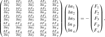
We use the multidimensional Newton–Raphson method (see Press 2007, Sect. 9.6) to solve this nonlinear system of joined statistical equilibrium, particle, and charge conservation equations by linearizing it to  or, in expanded form,
 (A.6)
(A.6)
where δn = (δn1, δn2, δn3, δnp, δne)⊤ is the column vector of corrections to unknowns, F = (F1, F2, F3, Fp, Fe)⊤ is the column vector of free terms given by Eqs. (A.1)–(A.5), and Ji, j = ∂Fi/∂nj is the Jacobian matrix with corresponding partial derivatives. As we already explained, one of the F1, F2, F3, or Fp equations is replaced by Eq. (A.3). We analytically compute the partial derivatives in a fashion similar to Leenaarts et al. (2007, see Appendix A).
This linear algebraic system of five equations with five unknowns is solved for the corrections δn using a standard Gaussian elimination scheme and the unknowns are updated to n + δn. The initial values of n are taken from the previous M-ALI iteration and are used to initialize F and  . The process is sub-iterated until the relative change in max|δn| reaches the desired tolerance of 10−4. At each sub-iteration, only the radiative bound-bound rates Ri, j are kept fixed, the remaining rates and the ionization fractions, which depend on ne, are updated accordingly. Algorithm 1 outlines the entire scheme.
Initialize n using the LTE approximation.
repeat // M-ALI iterations
Get background opacities, emisivities, and absorption
profiles from ne as well as foreground opacities and
emisivities from ni and np.
Integrate the transfer equation for the radiation field.
Re-evaluate and fix radiative bound-bound rates Ri,j.
repeat // non-LTE charge conservation iterations
Re-evaluate radiative and colllisional rates dependend on
ne: bound-free, Ri,p(ne), Rp,i(ne), Ci,p(ne), Cp,i(ne), and
bound-bound Ci,j(ne).
Get the ionization fractions fs,i(ne, T).
Compute F and  from n and the rates.
Solve the system (A.6) for δn.
n ← n + δn
until max |δn|/|n| < 10−4
until converged n
All Figures
|
Fig. 1. Illustration of the model atmosphere. Panel a: vertically emergent intensity in the 5000 Å continuum. Panel b: vertical magnetic field strength where the optical depth at 5000 Å is unity. Panel c: lowest height of the first occurrence of a temperature of 0.5 MK. The zero point of the height scale is defined as the average height of where the optical depth at 5000 Å is unity over a weakly magnetized patch. The red areas in panel c show where the CME arm is located in the original model atmosphere. |
| In the text | |
|
Fig. 2. Simulated images of Hα at nominal line center, Δλ = 0 Å, from the model atmosphere in vertically emergent intensity. The images are given in brightness temperature Tb and are clipped at 2.8 and 8.5 kK. Panel a: 1.5D radiative transfer where each column in the snapshot is treated as a plane-parallel atmosphere. Panel b: full 3D radiative transfer. The minimum, maximum, and average Tb for the entire field of view (FOV) is provided in a label above each panel. |
| In the text | |
|
Fig. 3. Observations of two active regions close to the disk center at the nominal line center of (a) Ca II K (SST/CHROMIS), (b) Hα (SST/CRISP), (c) Ca II 8542 Å (SST/CRISP), and (d) Mg II k (IRIS). Panels a–c: NOAA 12593. Panel d: NOAA 12494. The images are given in brightness temperature Tb and are clipped at 4.5–6 K for Ca II K, 3.9–6 Kk for Hα, 3.8–6 kK for 8542 Å, and 4.7–7 kK for Mg II k. Above the top left corner of each panel we show the minimum, maximum, and average brightness temperature for the FOV. Panels a–c have the same coordinate scale, while panel d has a different scale. |
| In the text | |
|
Fig. 4. Dependence of the vertically emergent intensity in Mg II k on how the electron density is computed. Panel a: spatially averaged relative change in the intensity, which is computed using either non-LTE or LTE electron densities. Panels b,c: line intensities expressed as brightness temperature Tb and computed using LTE (blue) or non-LTE (red) electron density at two structures indicated in Fig. 7. Panel b: dark fibril, red dot in Fig. 7. Panel c: flare ribbon, blue dot in Fig. 7. |
| In the text | |
|
Fig. 5. Distribution of the differences between the line-core formation heights of Hα and, respectively, Mg II k (blue), Ca II K (green), and Ca II 8 542 Å (orange). |
| In the text | |
|
Fig. 6. Fraction of an element in a given ionization state for Mg II (blue solid), Ca II (green solid), and H I (red solid) in a column of the MURaM model atmosphere. Panel a: log-scaled ionization fractions. Panel b: linearly scaled ionization fractions. Panel c: gas temperature (black solid) as a function of height. Vertical lines show the maximum formation heights of Mg II k (dashed blue), Ca II K (dashed green), and Hα (dashed red). |
| In the text | |
|
Fig. 7. Simulated images of Ca II 8542 Å, Ca II K, Mg II k, and Hα from the model atmosphere in vertically emergent intensity. Top row: at nominal line center, Δλ = 0 Å. Bottom row: at wavelengths corresponding to the maximum formation height, maxz(τ = 1). Intensity is expressed as brightness temperature Tb and is clipped to same ranges in each column: 3.6–7 kK for Ca II 8 542 Å, 3.6–7 kK for Ca II K, 3.6–8 kK for Mg II k, and 3.6–10 kK for Hα. The minimum, maximum, and average Tb for the entire FOV is provided in a label above each panel. Colored symbols indicate the following structures: a dark fibril (red dot) and a flare ribbon (blue dot), see Fig. 4; an active region in emission (orange cross), see Fig. 12; an active region in emission with a strong velocity gradient (blue cross), see Fig. 13; a sunspot (green cross), see Fig. 14; a fibril (red cross), see Fig. 15. |
| In the text | |
|
Fig. 8. Image of Hα at nominal line center overplotted with the horizontal magnetic field directions (orange arrows) at the formation height. The arrows are plotted every 30th grid point. The visibility of Hα fibrils is artificially enhanced using unsharp masking. The blue and red lines indicate two slices along selected fibrils illustrated in Figs. 9 (blue) and 10 (blue and red). |
| In the text | |
|
Fig. 9. Mass density in a vertical cut through the model atmosphere along the blue line in Fig. 8. For each spectral line mentioned in the legend, corresponding dashed curves show the maximum formation height at optical depth unity. The white dotted line shows the first occurrence from the upper convection zone where the magnetic pressure equals gas pressure (β = 1). The arrows show the direction of the magnetic field vector in the plane of the cut along the formation height curve of Hα. These arrows are plotted every tenth grid point. |
| In the text | |
|
Fig. 10. Alignment between the magnetic field vector and the curve of the maximum formation height at optical depth unity in two selected vertical slices. Left column: blue curve fibril in Fig. 8. Right column: red curve fibril in Fig. 8. Top row: formation heights of Hα (red) and Ca II 8542 Å (blue) with the β = 1 height (white dotted) layered over the mass density (grayscale background). Middle row: angle between the inclination of the magnetic field and the τ = 1 curve. Bottom row: angle between the magnetic field azimuth and the azimuth of the fibril. |
| In the text | |
|
Fig. 11. Spatially averaged line profiles of Ca II 8542 Å, Ca II K, Mg II k, and Hα expressed as brightness temperature Tb for the model atmosphere and our observations. Blue: observations; red: model atmosphere at full resolution; green dashed: model atmosphere spectrally degraded to match the resolution of the observations. Panels a–d: spatial averages for the entire model FOV. Panels e–h: spatial averages for a weakly magnetized patch only. The Hα and Mg II k lines are not degraded spectrally. |
| In the text | |
|
Fig. 12. Line formation in a flare ribbon (orange cross in Fig. 6). Top row: profiles of vertically emergent intensity, expressed as brightness temperature Tb, as function of frequency from line center (in Doppler shift units) for Ca II 8542 Å (orange), Ca II K (green), Mg II k (blue), and Hα (red). Bottom left: line source functions for Hα (red dashed) and Ca II 8542 Å (orange dashed), expressed as excitation temperature, and the gas temperature (solid black) as a function of column mass. Bottom middle: photon destruction probabilities for each of the lines. Bottom right: height of optical depth unity (solid colored) and the vertical velocity (solid black dots indicate the grid points, upflow is positive) as a function of frequency from line center in Doppler shift units. |
| In the text | |
|
Fig. 13. Line formation in a flare ribbon with strong velocity gradient (blue cross in Fig. 6). The figure follows the same format as Fig. 12. |
| In the text | |
|
Fig. 14. Line formation in a sunspot (green cross in Fig. 6). The figure follows the same format as Fig. 12. |
| In the text | |
|
Fig. 15. Line formation in a fibril (red cross in Fig. 6). The figure follows the same format as Fig. 12. |
| In the text | |
Current usage metrics show cumulative count of Article Views (full-text article views including HTML views, PDF and ePub downloads, according to the available data) and Abstracts Views on Vision4Press platform.
Data correspond to usage on the plateform after 2015. The current usage metrics is available 48-96 hours after online publication and is updated daily on week days.
Initial download of the metrics may take a while.