| Issue |
A&A
Volume 628, August 2019
|
|
|---|---|---|
| Article Number | A135 | |
| Number of page(s) | 16 | |
| Section | Extragalactic astronomy | |
| DOI | https://doi.org/10.1051/0004-6361/201935874 | |
| Published online | 20 August 2019 | |
Testing the disk-corona interplay in radiatively-efficient broad-line AGN
1
Max-Planck-Institut für Extraterrestrische Physik (MPE), Giessenbachstrasse 1, 85748 Garching bei München, Germany
e-mail: This email address is being protected from spambots. You need JavaScript enabled to view it.
2
INAF-Osservatorio Astronomico di Brera, Via Bianchi 46, 23807 Merate, LC, Italy
Received:
12
May
2019
Accepted:
18
July
2019
Abstract
The correlation observed between monochromatic X-ray and UV luminosities in radiatively-efficient active galactic nuclei (AGN) lacks a clear theoretical explanation despite being used for many applications. Such a correlation, with its small intrinsic scatter and its slope that is smaller than unity in log space, represents the compelling evidence that a mechanism regulating the energetic interaction between the accretion disk and the X-ray corona must be in place. This ensures that going from fainter to brighter sources the coronal emission increases less than the disk emission. We discuss here a self-consistently coupled disk-corona model that can identify this regulating mechanism in terms of modified viscosity prescriptions in the accretion disk. The model predicts a lower fraction of accretion power dissipated in the corona for higher accretion states. We then present a quantitative observational test of the model using a reference sample of broad-line AGN and modeling the disk-corona emission for each source in the LX − LUV plane. We used the slope, normalization, and scatter of the observed relation to constrain the parameters of the theoretical model. For non-spinning black holes and static coronae, we find that the accretion prescriptions that match the observed slope of the LX − LUV relation produce X-rays that are too weak with respect to the normalization of the observed relation. Instead, considering moderately-outflowing Comptonizing coronae and/or a more realistic high-spinning black hole population significantly relax the tension between the strength of the observed and modeled X-ray emission, while also predicting very low intrinsic scatter in the LX − LUV relation. In particular, this latter scenario traces a known selection effect of flux-limited samples that preferentially select high-spinning, hence brighter, sources.
Key words: galaxies: nuclei / quasars: general / quasars: supermassive black holes / X-rays: general / accretion / accretion disks / galaxies: active
© R. Arcodia et al. 2019
 Open Access article, published by EDP Sciences, under the terms of the Creative Commons Attribution License (http://creativecommons.org/licenses/by/4.0), which permits unrestricted use, distribution, and reproduction in any medium, provided the original work is properly cited.
Open Access funding provided by Max Planck Society.
1. Introduction
The development of an in-depth understanding of accretion physics in active galactic nuclei (AGN) has tended to lag behind in comparison to other accreting objects (e.g., X-ray binaries, cataclysmic variables, and protoplanetary disks), for which many more observational constraints are available. While it seems that the standard thin-disk model (Shakura & Sunyaev 1973, hereafter SS73) is not able to fully explain the plethora of accreting sources that we observe (e.g., Koratkar & Blaes 1999; Blaes 2007; Antonucci 2015), it is still unclear to what extent this simple but effective prescription has to be improved (Kishimoto et al. 2008; Capellupo et al. 2015, 2016).
Since the first AGN X-ray spectral surveys were performed (e.g. Elvis et al. 1978; Turner & Pounds 1989), the need for an additional spectral component to extend the cold-disk’s ≲ keV temperatures was evident. This so-called X-ray “corona” (e.g. Liang & Price 1977; Galeev et al. 1979) is now almost universally considered as a hot (∼109 K), optically thin (τ ≲ 1) plasma up-scattering the disk photons via thermal Comptonization (Haardt & Maraschi 1991, 1993; Haardt et al. 1994; Stern et al. 1995), although an additional warm component is sometimes needed to fit the softest X-rays (Petrucci et al. 2018; Kubota & Done 2018, and references therein). The proximity of the corona to the central black hole was immediately suggested by its strong and fast variability (e.g. McHardy 1989) and by the reflection signatures (Lightman & White 1988; Pounds et al. 1990; Nandra et al. 1991; Williams et al. 1992; Tanaka et al. 1995), but in-depth information regarding its geometry and formation mechanism is still lacking.
The geometry of the corona can be constrained via the observation of X-ray reverberation lags (Fabian et al. 2009, 2017; De Marco et al. 2013; Uttley et al. 2014), that seem to show a, possibly non-static, corona extending vertically and radially over the underlying disk for a few and a few tens of gravitational radii, respectively (Wilkins et al. 2016). The compactness of the corona and the origin of the X-rays close to the black hole also appear to be confirmed by micro-lensing results (e.g. Mosquera et al. 2013; Reis & Miller 2013).
As far as the formation of the corona is concerned from the theoretical point of view, the most likely explanation for it is that it is magnetically-dominated with an efficient saturation of the magnetic field that is amplified via the magneto-rotational instability (MRI, Chandrasekhar 1960; Balbus & Hawley 1991, 1992; Hawley & Balbus 1991, 1992) and extending buoyantly upward (and downward) from the denser parts of the disk (Galeev et al. 1979; Stella & Rosner 1984; Di Matteo 1998; Merloni & Fabian 2002; Blackman & Pessah 2009). Magnetic reconnection can then keep the corona hot (e.g., Liu et al. 2002; Uzdensky & Goodman 2008; Uzdensky 2016; Beloborodov 2017; Werner et al. 2019; Ripperda et al. 2019). This scenario seems to be supported by magneto-hydrodynamic (MHD) simulations (Miller & Stone 2000; Uzdensky 2013; Bai & Stone 2013; Jiang et al. 2014; Salvesen et al. 2016; Kadowaki et al. 2018), although only qualitative comparisons with observations have been made so far (however, see Schnittman et al. 2013). Much effort has, nonetheless, been put into trying to shed light on the physics of the disk-corona system (see Blaes 2014) and this will continue with global 3D radiation-MHD simulations (e.g. Jiang et al. 2017a), that are now approaching sub-Eddington flows as well (Jiang et al. 2019).
Observationally, the increase in quality and quantity of available AGN X-ray-to-UV data from large samples can provide insightful, and more easily approachable, diagnostics. The smoking gun of the disk-corona interplay in radiatively efficient AGN is given by the non linear correlation observed between the 2 keV and 2500 Å monochromatic luminosities (e.g., Vignali et al. 2003; Strateva et al. 2005; Steffen et al. 2006; Young et al. 2009; Lusso et al. 2010; Lusso & Risaliti 2016, and references therein), that persists throughout the common observed X-ray and optical-UV bands (Jin et al. 2012). Despite the possible differences arising from different sample selections and regression techniques, most observations point towards a log LX − log LUV correlation with a slope ≈0.6, a dispersion that can be as small as σ ≈ 0.2 dex (Lusso & Risaliti 2016; Chiaraluce et al. 2018), and no apparent redshift dependency. Such a tight correlation paved the way for quasars to provide an alternative standard candle for cosmographic studies (Risaliti & Lusso 2015, 2019). The slope, being smaller than unity, indicates that from lowly to highly accreting AGN, the disk emission increases more than the corona emission (e.g., Kelly et al. 2008) with crucial implications for the physics governing the coupled disk-corona system. However, a solid and conclusive theoretical explanation, for what is one of the most studied multi-wavelength observables in AGN, is still lacking.
The goal of this paper is indeed to test a self-consistently coupled disk-corona analytic model against the observed LX − LUV. Given the existing gap between simulations and observations, we argue that the use of simplified (but motivated) prescriptions still represents a powerful tool to explain observed disk-corona scaling relations, as it was done with the X-ray photon index (or the X-ray bolometric correction) correlation with the Eddington ratio (Wang et al. 2004, 2019; Cao 2009; Liu & Liu 2009; You et al. 2012; Liu et al. 2012, 2016a), or with the log LX − log LUV itself (Lusso & Risaliti 2017, hereafter LR17; Kubota & Done 2018). We here rely uniquely on the log LX − log LUV relation, since monochromatic LX and LUV values can be directly obtained from spectral fits. Forward modeling monochromatic luminosities circumvents difficulties and issues typical of model comparisons with accretion rate, Eddington ratio or bolometric luminosity estimates (e.g., Richards et al. 2006; Davis & Laor 2011; Slone & Netzer 2012; Krawczyk et al. 2013; Capellupo et al. 2015, 2016; Kilerci Eser & Vestergaard 2018).
We describe our disk-corona model in Sect. 2 (and Appendix A) and we briefly show its qualitative predictions in Sect. 3. Then, we outline the observational test that we put forward to thoroughly understand the disk-corona interplay in Sect. 4 and we show the results in Sect. 5. Throughout this work, we quote median values with 16th and 84th percentiles unless otherwise stated.
2. The disk-corona model
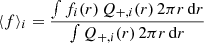
The disk-corona model adopted in this work is largely based on the prescriptions put forward by Merloni (2003, hereafter M03; see also Merloni & Fabian 2002, 2003), in which the standard conservation equations of a geometrically-thin and optically-thick accretion disk (SS73; Pringle 1981) are self-consistently coupled with the X-ray corona, indicated as the fraction f (e.g., Haardt & Maraschi 1991; Svensson & Zdziarski 1994) of accretion power (per unit area, Q+) that is dissipated away from the cold disk (e.g., Stella & Rosner 1984; Di Matteo 1998):
 (1)
(1)
with Qcor = vDPmag and  , where vD is the vertical drift velocity (taken proportional to the Alfvén speed via an order-unity constant b), Pmag = B2/8π is the magnetic pressure, cs is the sound speed and τrϕ is the vertically-averaged stress tensor.
The stress tensor can be assumed to be dominated by Maxwell stresses (e.g., Hawley et al. 1995; Sano et al. 2004; Minoshima et al. 2015), from which we can write τrϕ = k0Pmag, with k0 being a constant of order unity (Hawley et al. 1995). To build a self-consistent solution to the accretion problem, we need to relate the stress tensor (via the magnetic pressure) with local quantities that standard analytic models are familiar with. As a matter of fact, the α−prescription is not the only educated guess that is adopted to dodge our ignorance of the physical mechanism producing the disk viscosity. Within the same theoretical framework, fundamental modifications to the viscosity law can be introduced depending on whether the viscous stress is assumed to scale proportionally with the total (Ptot, gas plus radiation) pressure (SS73), with the gas pressure alone (Lightman & Eardley 1974; Sakimoto & Coroniti 1981; Meyer & Meyer-Hofmeister 1982; Stella & Rosner 1984) or with the geometric mean of the two (M03; Ichimaru 1977; Taam & Lin 1984; Burm 1985). It was soon discovered that the first prescription leads to thermally and viscously unstable disks in the radiation-pressure dominated regions, with the first instability acting on shorter timescales (Lightman & Eardley 1974; Shakura & Sunyaev 1976; Pringle 1976). This encouraged many authors (Hoshi 1985; Szuszkiewicz 1990; Merloni & Nayakshin 2006; Grzȩdzielski et al. 2017a) to generalize the viscosity law. Recent simulations (albeit of gas-pressure dominated disks only) indeed seem to show a power-law stress-pressure relation (Sano et al. 2004; Minoshima et al. 2015; Ross et al. 2016; Shadmehri et al. 2018), with an index varying from zero to one according to the different assumptions.
Here, we address this issue generalising the model reported in M03 with:
 (2)
(2)
where α0 is a constant, generally not equal to αSS73 = Pmag/Ptot. This behavior is physically motivated by the MRI prescriptions, as its growth rate was shown to depend on the Prad-to-Pgas ratio (Blaes & Socrates 2001; Turner et al. 2002) influencing the level of the magnetic field saturation. Equations (1) and (2) provide the closure equation of the disk-corona system:
 (3)
(3)
where k1 = 3k0/2b gathers the model’s uncertainties in an order unity factor (M03). Its exact value only affects f at its maximum  and not the nature of what is described throughout this paper.
The model is then completed with the equation of state:
 (4)
(4)
and with a density- and temperature-dependent opacity κ = κ (ρ, T). We compute the opacity value self-consistently with the density and temperature at each radius with an iterative process, using as reference stellar opacity tables (at solar metallicity) from the Opacity Project (Seaton et al. 1994; Seaton 1995). This is important since the density and temperature regimes relevant for AGN disks imply opacities that can be significantly different from the electron scattering value (e.g., see Jiang et al. 2016; Czerny et al. 2016; Grzȩdzielski et al. 2017b).
Further, we assume a downward component of the X-ray emission (η) and a disk albedo (adisk), which modify the disk equations from the usual (1 − f) factor (M03; Svensson & Zdziarski 1994) to:
![Mathematical equation: $$ \begin{aligned} 1-\tilde{f}=1-f\left[1-\eta \left(1-a_{\rm disk}\right)\right] \end{aligned} $$](/articles/aa/full_html/2019/08/aa35874-19/aa35874-19-eq7.gif) (5)
(5)
We here adopt η = 0.55 and adisk = 0.1, respectively (e.g., Haardt & Maraschi 1993). These are typical values for anisotropic Comptonization in plane-parallel geometry, although more generally the product η(1−adisk) can be a function of the photon index Γ (Beloborodov 1999; Malzac et al. 2001) and of the disk’s vertical structure.
For simplicity, we adopt dimensionless units for the black hole mass, the accretion rate, the radial distance and the vertical scale-height:
 (6)
(6)
The equations for h, mid-plane ρ (g cm−3), P (dyn cm−2) and T (K), with the closure equation for f, are reported in Appendix A in Newtonian approximation (however, see Merloni & Fabian 2003, for a relativistic derivation of the μ = 0.5 case), along with the related radial profiles (Fig. A.1). We note that a constant efficiency of ϵ0 = 0.057, typical of non-rotating black holes, and a no-torque inner boundary condition ( , with r0 = 3 and rout = 2000) are initially adopted.
Once m, ṁ, α0, μ and fmax are fixed, one can numerically solve the closure equations for f at each radius (see the last rows of Eqs. (A.1) and (A.3), respectively). The left-hand side is equal to Prad/Pgas and we can infer the correct regime and compute the main physical quantities at the mid-plane (ρ, P, T, κ). Then, the effective temperature at the surface is computed:
 (7)
(7)
where we take τ(r)=h(r) ρ(r) κ(r). Monochromatic optical-UV luminosities can be then easily computed in the multi-color blackbody approximation:
 (8)
(8)
where π Bν(Teff) is the black-body flux at the frequency ν and temperature Teff(r).
In this framework, the energy per unit area dissipated in the corona at each radius is Qcor(r)=f(r)Q+(r), although only a fraction (1 − η) will contribute to what is observed as X-ray emission:
 (9)
(9)
Here, we did not include the component reflected by the disk (given by the fraction f η adisk), so that we could easily extrapolate at each radius a monochromatic value, for instance L2 keV, assuming a simple power-law spectrum within νi = 0.1 and νf = 100 keV:
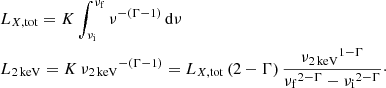 (10)
(10)
The model relies on the assumption that a plane-parallel geometry holds for bright radiatively-efficient sources, lying in a sweet spot of accretion rate (ṁ approximately from a few percent to Eddington). Hence, the accretion disk extends down to the innermost stable circular orbit (ISCO) and no advection is included. A scripted version of the model outlined in this section will be made publicly available online1.
2.1. Radial profiles for f and L2 keV
In Fig. 1 we show as an example radial profiles of f and L2 keV, obtained by solving Eqs. (A.1), (A.3), (9) and (10). For simplicity, we fixed α0 = 0.02 and fmax = 0.5 and used the three values of μ corresponding to the most-used viscosity laws, namely μ = 0, 0.5 and 1, for Pmag proportional to Ptot,  and Pgas, respectively. Other values of μ would support the same picture with analogous intermediate profiles. A range of typical m, ṁ and X-ray spectral slopes was chosen, following the distribution of objects observed in the survey field adopted for the observational test (see Sect. 4 below), namely with median values (and related 16th and 84th percentiles) of
  ,
,  and Γ = 2.1 ± 0.1.
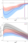 |
Fig. 1. Radial profiles for the fraction f of power dissipated in the corona (top panel) and L2 keV (bottom panel), obtained with fixed α0 = 0.02 and fmax = 0.5. Colors are coded according to the choice of the viscosity law: stress proportional to Ptot (Pgas + Prad, μ = 0, black), to Pgas (μ = 1, blue), or the geometric mean of the two (μ = 0.5, red). The continuous solid, or solid-dashed, lines represent the median profiles, with the related shaded areas showing the 16th and 84th percentiles, the scatter due to the range of sources (i.e. m and ṁ) modeled. L2 keV is proportional to the product of f and Q+ (the accretion power per unit area). As Q+ has very similar profiles across all models, those systems for which f is smaller produce weaker coronae in the central part. Top panel: a solid line for the median f-profile represents (thermally) stable regions of the median test source, whereas a dashed line highlights the instability regions. The vertical dot-dashed lines show instead where the median transition radius, from Prad- to Pgas-dominated regions, lies. Refer to Sect. 2.1 for details. |
The solid (or solid-dashed) lines represent the median profiles, with the corresponding shaded areas showing the 16th and 84th percentiles of the distribution. The top panel of Fig. 1 shows how the standard μ = 0 law (e.g., SS73) results in f = fmax at all radii (e.g., Svensson & Zdziarski 1994), whereas alternative viscosity laws (e.g., μ = 0.5 and μ = 1) show non-constant radial profiles for f: in the latter cases, the fraction of power dissipated in the corona is smaller in the regions strongly dominated by Prad. As it was shown in M03 in particular for the μ = 0.5 scaling, the higher suppression of the growth rate in Prad-dominated regions of the disk leads to such damped f-profiles. This directly influences the strength of the corona emission, as L2 keV is proportional (through LX, tot) to the product of f and Q+: Q+ peaks at small radii in a very similar way across all models, therefore the ones with deeper f-profiles show flatter L2 keV radial profiles and, hence, weaker coronae (bottom panel of Fig. 1). The exact shape of f(r) also affects the strength of the disk emission since the two are self-consistently coupled (see Eq. (5)).
We can also define the mean value of each f(r) profile (i.e. for each combination of m, ṁ and Γ):
 (11)
(11)
that is also a function of μ, α0 and fmax. Then, the mean value can be computed for the median f profiles in the examples in the top panel of Fig. 1: ⟨f⟩median = 0.5, 0.13 or 0.05, for μ = 0, 0.5 and 1, respectively. Of course, within such a model the exact value of ⟨f⟩median depends on its normalization fmax, that is a free parameter in the model only bound to be < 1. Nonetheless, simply from looking at ⟨f⟩median as a function of μ (and from Fig. 1) we can see how, for the same set of inputs (e.g., m, ṁ), the different accretion prescriptions relate to the output corona luminosities: in a nutshell, going from μ = 0 to μ = 1 produces lower ⟨f⟩median, thus weaker coronae.
Changing μ also affects the logarithmic scatter in the radial profiles, from being absent in μ = 0 to increase with μ for μ ≠ 0 (see Fig. 1). The spread on a given f(r) is due to the scatter in m, ṁ and Γ, where the major role is played by the accretion rate (e.g., see Fig. 1 in M03). Crucially, ⟨f⟩ decreases with increasing ṁ for all μ ≠ 0 models. This points in the same direction as the evidence of an X-ray bolometric correction (that is proportional to the inverse of f) increasing with the accretion rate (e.g. Wang et al. 2004; Vasudevan & Fabian 2007, 2009; Lusso et al. 2010; Young et al. 2010). This relation between ⟨f⟩ and ṁ has also crucial implications for what our models predictions on the physical mechanisms behind the observed LX − LUV (see Sect. 3).
2.2. Local thermal stability
Before proceeding to a detailed observational test of the model, we briefly discuss here the stability issue for the various adopted viscosity laws. Jiang et al. (2016) showed that the presence of the iron bump in the opacity at ∼2 × 10⁵ K stabilizes the flow in the disk regions around that temperature, where the cooling term has a different dependency and thermal runaway is avoided (Grzȩdzielski et al. 2017b). In the top panel of Fig. 1, a solid median line for the f-profile represents (thermally) stable regions of the median test source, whereas a dashed line highlights the instability regions. The vertical dot-dashed lines show instead where the median transition radius, from Prad- to Pgas-dominated regions, lies. This highlights that, for the median test source, the stability region extends also well within Prad-dominated regions of the disk, confirming previous results (Jiang et al. 2016; Grzȩdzielski et al. 2017b). More quantitatively, we computed the thermal stability balance (e.g. Pringle 1976) for each test source (m, ṁ) at all radii with varying viscosity laws. The new stability regions in the inner Prad-dominated portions of μ = 0 and μ = 0.5 disks are ubiquitous, but they appear at different radii according to where the disk reaches the temperatures around the iron bump in κ (see also Fig. A.1). The μ = 1 case, as it is well known (e.g. Lightman & Eardley 1974), is stable throughout.
3. Predictions of the model on the LX − LUV relation
In this section we aim to test our disk-corona model (presented in Sect. 2) against the observed LX − LUV, a robust observable linked to the disk-corona physics. Before performing a more quantitative observational test (Sect. 4), we here outline the predictions of our model concerning the disk-corona energetics and the expected impact of our accretion prescription on the LX − LUV.
The schematic illustration in Fig. 2 summarizes the qualitative take-home messages of this work. The observed LX − LUV states that going from a lower to a higher accretion regime, the luminosity of the corona increases less than the disk luminosity, resulting in a slope smaller than one in the log-space. In our model for the disk-corona system, the luminosity outputs are directly modified by the viscosity prescription in the flow, determined by the parameter μ, and by the fraction of accretion power going into the corona, f (see Table 1 for a summary on the model parameters). Among all scenarios spanned by these two main unknowns, the qualitative behavior of the accretion disk-corona system, along its radial extent, is similar: higher accretion states have a more powerful disks and coronae, but wider Prad-dominated inner region and, only for modified viscosity prescriptions (i.e. μ ≠ 0), lower relative contribution of the corona to the total luminosity (see the upper diagram in Fig. 2).
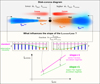 |
Fig. 2. Schematic illustration of our model and how it relates to the observed LX − LUV (see Sect. 3 for an interpretative guide). |
Summary of recurring model parameters.
Thus, our model can provide a simple explanation for the observed slope of the LX–LUV relation, bridging in a simple but effective way the gap between the observed X-to-UV energetics and some aspects of MRI simulations. Changing μ not only affects the disk thermodynamics, but also changes the amount of power carried away by the corona (see Fig. 1). A constant radial profile for f (e.g., Svensson & Zdziarski 1994; here μ = 0) would naturally result in a LX − LUV close to a one-to-one relation. On the contrary, the alternative viscosity prescriptions, that we identify with μ ≠ 0, inherently result in a different disk-corona energetic coupling for varying accretion rates: in particular, higher ṁ yield more damped f−profiles (see also M03). In this scenario, the outcome would be a slope of the LX − LUV that is smaller than one (see the lower diagram in Fig. 2).
It is worth stressing that it is only the relative fraction f that is more suppressed in the inner regions of systems with a modified viscosity and not the X-ray emission per se. Regardless the underlying assumption of a plane-parallel geometry for the disk-corona system (see Eq. (5)), the X-ray emission peaks in the innermost radii (e.g., see the μ = 0.5 case in Fig. 1). This will be addressed in details in Sect. 5.1.
Figure 3 shows an example of a mock LX − LUV from the model realizations, with fmax = 0.5 and different values of μ as in Fig. 1, with the same color coding. For the connected solid points, a single typical mass (log m = 8.7) is adopted, with increasing ṁ = 0.03, 0.07, 0.17, 0.42, 1 (from left to right in LUV). The relation is linear for a given mass, with the dashed lines indicating a slope of one to guide the eye. As qualitatively shown in the illustrative Fig. 2, models where f is constant in radius and in accretion state (black points) yield a slope close to one (even higher for the single mass); instead, alternative viscosity prescriptions (red and blue), that change the disk-corona energetic interplay via f(r), show a flatter slope. The underlying transparent points show the mock LX − LUV for a distribution of  ,
,  and Γ = 2.1 ± 0.1, that follows the typically observed objects (see Sect. 4).
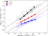 |
Fig. 3. Mock LX − LUV with fixed fmax = 0.5 and different μ color coded, as in Fig. 1. The connected solid points show the trend of a single typical mass (log m = 8.7) with ṁ = 0.03, 0.07, 0.17, 0.42, 1 (increasing from left to right in LUV). The dashed lines indicate a slope of one. The distributions of transparent points show the mock LX − LUV for a range of |


4. Observational test: modeling the LX − LUV
In the previous section we qualitatively outlined what are the physical mechanisms identified as the origin of the observed slope smaller than one. A more quantitative test is needed to thoroughly investigate all aspects of the observed LX − LUV, including its normalization and intrinsic scatter. The exact value of the slope given by the models not only depends on the unknowns μ, fmax and α0, but also on the details of the distributions of m, ṁ, Γ that are adopted for the calculations. Nonetheless, not all combinations of these three parameters are observed, because they do not exist in nature or we are biased against their detection (for example, the black masses of AGN follow a given mass distribution, some some mass ranges are more probable than others in any observed sample). That is why we select a reference sample of radiatively-efficient broad-line AGN (Sect. 4.1) and model the most likely values for m, ṁ, Γ for each source individually, based on the available data.
4.1. The reference sample of broad-line AGN
We built our reference sample starting from the 1787 AGN within the XMM-XXL north survey (Pierre et al. 2016) identified as broad-line AGN (BLAGN) by the Baryon Oscillation Spectroscopic Survey (BOSS) follow-up (Menzel et al. 2016; Liu et al. 2016b, hereafter L16). The X-ray spectral analysis on these sources was performed in L16 with the Bayesian X-ray Analysis software (BXA, Buchner et al. 2014), providing NH values, photon indexes (Γ) and the rest-frame 2 − 10 keV intrinsic luminosities (L2 − 10 keV). Furthermore, single-epoch virial black hole masses (MBH, e.g. Shen et al. 2008) and continuum luminosities (at 1350, 1700, 3000 and 5100 Å) were obtained on the BOSS spectroscopy with a fitting pipeline (for details, we refer to L16; Shen & Liu 2012). Luminosities were computed in L16 assuming H0 = 70 km s−1 Mpc−1, Ωm = 0.27 and ΩΛ = 0.732.
Then, we applied some cleaning criteria to avoid, as much as possible, imprecise estimates for the intrinsic (accretion-powered) LX and LUV and to remain consistent with what is computed by the model. Firstly, among the monochromatic luminosity values available in the optical-UV from L16 we adopted L3000 Å, obviously inducing a redshift cut in the sample (see Fig. B.1). Model wise there is no difference in computing L3000 Å or the more standard L2500 Å, and Jin et al. (2012) showed compatible correlations between the X-ray luminosity and each wavelength of the optical spectrum, although their coverage starts from 3700 Å. We verified a posteriori that this choice does not affect significantly the slope of the LX − LUV or the conclusions of our work.
Secondly, despite being defined as BLAGN, Liu et al. (2018) found that a fraction of these sources shows continuum reddening probably due to intervening dust along the line of sight, not accounted for by our model. Liu et al. (2018) defined a slope parameter α′ for the optical-UV continuum, to discern between the reddened sources and the bulk of blue BLAGN at each redshift. The contamination from extinction at L3000 Å was minimized by conservatively selecting sources with α′< − 0.5 (see Liu et al. 2018, their Fig. 2).
Moreover, the XMM-XXL survey has a typical exposure time of ∼10 ks per pointing (L16; Pierre et al. 2016). Here, the analysis was restricted to sources with at least 10 counts in the EPIC-pn (Strüder et al. 2001) and EPIC-MOS (Turner et al. 2001) cameras on board XMM-Newton (Jansen et al. 2001), to exclude sources with extremely low-quality X-ray spectra.
Then, to exclude data contaminated by X-ray absorption, not accounted for in our modeling, we conservatively selected only sources in which the 84th percentile of the NH posterior distribution was smaller than 1021.5 cm−2, a value typically adopted to distinguish X-ray obscured and un-obscured sources (Merloni et al. 2014; see also Della Ceca et al. 2008).
Finally, we take L2 keV as reference for the corona emission in the LX − LUV. In the model, we computed mock LX, tot with no reflection, so that we could easily extrapolate L2 keV assuming a simple power-law spectrum. However, in L16 the reflection component was also included in the calculation of L2 − 10 keV, as it is usually observed both in low-z (e.g. Nandra et al. 2007) and high-z (e.g. Baronchelli et al. 2018) spectra (see the average-AGN model in Buchner et al. 2014). Therefore, we consistently excluded from the analysis all the sources with a significant reflection component: given the high errors of the typical log R fit in L163, we included only sources in which the 16th percentile was < − 0.2 and the 84th was < 0.5. We note that L16 included in the fit also a scattering contribution from ionized material inside the angle of the torus (see Buchner et al. 2014), although the fit normalizations are on the order of 10−4 with respect to the main power-law component.
The final cleaned subsample, to which we will refer as XMM-XXL, consists of 379 sources with observed m (with median  ), L3000 Å, Γ (with median Γ = 2.1 ± 0.1) and L2 keV. In Fig. 4 we show the
  relation, with the best-fit linear regression given by:
 (12)
(12)
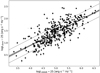 |
Fig. 4. LX − LUV relation of the 379 bright BLAGN of XMM-XXL. Monochromatic luminosity values are here scaled by 25 dex, to ease the comparison with recent works. The solid black line is the median regression line obtained with emcee, with the corresponding 16th and 84th percentiles represented with the shaded gray area. The dashed black lines show the intrinsic scatter around the median relation. |
with intrinsic scatter σintr = 0.27 ± 0.01. Linear regressions in two (or more) dimensions were performed with emcee (Foreman-Mackey et al. 2013), accounting for uncertainties on all variables and an intrinsic scatter using the likelihood provided in D’Agostini (2005). The uncertainty in the independent variable(s) is propagated with the derivative ∂Y/∂X calculated in X (Xi), equal to the slope coefficient(s) in the linear case (D’Agostini 2003). The slope we measure is slightly flatter than what is quoted in the recent literature (e.g., Lusso & Risaliti 2016), although we did not consider all the possible biases of flux-limited samples (however, see Appendix B). For the main scope of this paper, it is sufficient to have a reference sample cleaned in accord with the physics described within the model.
4.2. Methodology of the observational test
In our model ṁ = λedd = Lbol/Ledd, although we do not take as reference also ṁ or λedd from L16: the former is interpolated from the mass and a monochromatic optical luminosity (Davis & Laor 2011), while the latter depends on a disk-luminosity estimate via Lbol. Both approaches are based on standard-disk assumptions or calculations and using those values within our non-standard disk models would be an inconsistency. One can also estimate Lbol applying bolometric corrections (BC) to the observed monochromatic optical-UV luminosities (Richards et al. 2006; Runnoe et al. 2012), although the many uncertainties in play (Krawczyk et al. 2013; Kilerci Eser & Vestergaard 2018) and the high scatter in the BCs (Richards et al. 2006; Lusso et al. 2012) discouraged us in relying on this approach. Then, for every source we iteratively obtain the ṁ value yielding a model L3000 Å consistent with the observed one within its errors (typically ∼0.01 dex). This approach is similar to the interpolation method put forward by Davis & Laor (2011), although we do it consistently for each different model, which is given by a choice of μ, α0 and fmax.
The methodology then consists in fixing μ, α0 and fmax (see Table 1 for a summary on the model’s parameters), which will be referred to as the model choice, within a discrete 3D grid in μ = [0, 0.2, 0.4, 0.5, 0.6, 0.8, 1], α0 = [0.02, 0.2] and fmax = [0.1, 0.2, 0.3, 0.5, 0.7, 0.9, 0.99]. Then, we take as input m, Γ and L3000 Å from the observed data, allowing us to solve the equations of the model for each source and compute ṁ and L2 keV values (see Sect. 2). For each observed source of the reference sample, every model in the 3D grid can provide a mock entry for the LX − LUV. A proper comparison requires uncertainties to be assigned on the mocks, as the observed m, Γ and L3000 Å come with their own measurement and systematic errors, where obviously the ∼0.4 − 0.5 dex systematics in the mass estimates (e.g. Shen 2013, and references therein) play the dominant role. As it is mentioned above, mock L3000 Å values converge to the related observed quantities within their errors, hence we conservatively fixed the mock δL3000 Å at the 90th percentile of the uncertainty distribution in the observed L3000 Å (i.e. ∼0.03 dex). In order to compute uncertainties for ṁ and L2 keV, we ran each model 200 times on the same source, extracting the input values (m, Γ and L3000 Å) from a normal distribution with mean and standard deviation taken from the observed quantities and their errors. Then, the uncertainty on ṁ and L2 keV is taken from the dispersion of the 200 runs.
5. Results of the observational test
For all the models on the discrete 3D grid in the μ, α0 and fmax parameter space (see Sect. 4.2 and Table 1), we fit the LX–LUV distribution with a log-linear relation  . Three examples are shown in Fig. 5 for μ corresponding to the known analytic viscosity prescriptions (see Sect. 2). Ideally, a model should reproduce the observed LX − LUV in both normalization and slope. However, we can start decomposing the problem in two parts: a good match in the normalization (
 ) would state that globally, for a given optical-UV luminosity distribution, the modeled corona emission was strong enough (see Sect. 5.1); instead, if the slope (
 ) is matched, then the model accurately describes how the coronal strength varies from lowly- to highly-accreting sources (see Sect. 5.2). Moreover, as it can be seen from the examples in Fig. 5, our models come with their one intrinsic scatter, given by different m and Γ at a fixed ṁ. This provides precious insights on the nature of the total observed scatter (see Sect. 5.3).
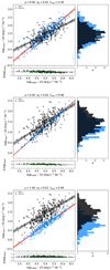 |
Fig. 5. The central panel of each image shows an example of the LX − LUV relation for both XMM-XXL (black stars) and the model (blue dots), in which the choice of μ, α0 and fmax is shown in the titles. The black and red solid lines are randomly drawn from the posterior distributions of normalization and slope for XMM-XXL and the model, respectively, with the median regression line thickened. The bottom panels show the residuals given by the difference of observed and mock log L2 keV and the right panels show the related distributions. The errors on the model are show in the bottom right corner of the central panels. |
5.1. The normalization of the LX − LUV
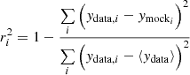
First, we investigate how well the mocks reproduce the data normalization along the vertical axis of the LX − LUV. To do so, we define a score for the goodness of match:
 (13)
(13)
The r2 score is computed drawing 1000 random samples from the observed log L2 keV within their errors (i.e. ydata, i), and 1000 random regression lines from emcee’s chains on the mock (i.e. ymocki). Then, the median and the 84th–16th inter-quantile range are quoted from the resulting distribution of 1000  scores. Negative scores indicate the data are poorly reproduced by the model; an r2 = 0 would be obtained by a constant value corresponding to the mean of the observed log L2 keV distribution. We can put a quality threshold and keep all the models that yield a positive score.
The r2 score as a function of fmax is shown in Fig. 6, where the choice of μ is color coded and the additional dependency on α0 is represented with varying line-types (it is minor or absent, as in μ = 0). We show for simplicity only values of μ corresponding to the known analytic viscosity prescriptions (see Sect. 2). The other values used would accordingly show intermediate results. For each viscosity law there is a preferred fmax, that fixes the maximum coronal strength in a model.
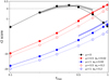 |
Fig. 6. r2 score, representing the goodness of match between XMM-XXL and mocks (see text), as a function of fmax. Models with μ = 0, 0.5, 1 are color coded in black, red and blue, respectively. The additional dependency on α0 is represented with varying line-types as shown in the legend, when present (it is absent for μ = 0). A good match is represented with a score greater than zero. The points include the uncertainties in the score values. The shaded areas represent the results obtained applying the same methodology on a different sample (RM-QSO, Liu et al., in prep.), fixing α0 = 0.02 and using the same colors. |
Models with higher μ need higher normalization fmax, since they have a comparably weaker X-ray emission, in accord with their lower ⟨f⟩median (see Fig. 1 and Sect. 2.1). Nonetheless, the law correspondent to μ = 1 does not produce adequately strong coronae even with fmax = 0.99 and can be ruled out (see right image in Fig. 5). Furthermore, μ = 1 produces a radially flatter X-ray emission profile (see bottom panel of Fig. 1), in contrast with observations that hint for coronae peaking in the inner radii (e.g. Mosquera et al. 2013; Reis & Miller 2013; Wilkins et al. 2016). We explore this behavior more quantitatively in the top panel of Fig. 7 showing how the radius of the annulus at which the 2 keV emission peaks (rpeak, or at which it is 90% of the total, r90) varies with μ: as μ increases, most of the corona emission comes from annuli placed at larger and larger radii.
 |
Fig. 7. Top panel: the 2 keV-emission rpeak (r90) as a function of μ is represented in black (gray). The green shaded area qualitatively shows the inner radii, where the bulk of X-ray emission is supposed to come from according to X-ray reverberation and micro-lensing. For increasing μ, the X-ray emission profile peaks at larger radii. Middle panel: for increasing μ the models obtain a slope of the LX − LUV closer to the observed one. The dark-green area represents the reference slope of the cleanest XXM-XXL (Appendix B), while the light-green refers to the slope quoted in LR17. Bottom panel: intrinsic scatter of the mock LX − LUV relations as a function of μ. The green area represents a tentative upper limit of the true scatter (Lusso & Risaliti 2016; Chiaraluce et al. 2018), that is only due to the physical properties of AGN. For simplicity, all panels show only the results obtained with a single fmax, corresponding to the highest r2-score (e.g., Fig. 6), and fixed α0 = 0.02. |
We also verified that our results do not depend on the sample adopted as reference. We performed the same analysis with the RM-QSO sources (Liu et al., in prep.; Shen et al. 2019), on which a similar analysis was performed and on which we applied compatible cleaning criteria and methodology, as described in Sects. 4.1 and 4.2. The results are shown in the r2 score plot (Fig. 6) with shaded areas, color coded for μ in the same way and using only α0 = 0.02. There is generally a good agreement between the two samples, suggesting that our results are not dependent from the different data used.
It is worth stressing that the fmax value at which each μ (possibly) matches the observed normalization is degenerate with the assumptions on the accretion efficiency and on the product η (1 − adisk). Namely, higher accretion efficiencies and/or a higher fraction of the coronal emission beamed away from the disk would increase the normalization of the LX–LUV relation, and shift all curves of Fig. 6 to the left. This will be further examined in Sects. 5.6 and 5.7.
5.2. The slope of the LX − LUV
Figure 6 allows us to track the models (i.e. combinations μ, α0 and fmax, see Table 1) that broadly reproduce the normalization  of the observed LX − LUV. Nonetheless, obtaining the correct normalization is simply a weighting exercise of the energetic outputs of the disk and the corona. It is the slope that carries the exact information on how the disk-corona interplay changes across the different accretion regimes of bright radiatively-efficient AGN (see Sect. 3). This would require a precise knowledge of the true slope of the LX − LUV. The observations suggest a value around ≈0.6 (Lusso & Risaliti 2016; LR17; our Appendix B) and we can acknowledge this value as reference. Our methodology, however, can be regarded as data-independent, and it would applicable even if future works will update the current knowledge on the exact value of the slope.
In the middle panel of Fig. 7 we show how the modeled slope of the of the LX − LUV gets closer to the observed one for increasing μ (i.e. for more damped radial f-profiles), for a fixed α0 = 0.02 and using only the fmax corresponding to the highest r2-score. This is because models with increasing μ have higher logarithmic scatter in f(r), meaning that going from lowly- to highly-accreting sources the span in ⟨f⟩i is larger, with high-ṁ objects having comparably weaker X-ray emission with respect to low-ṁ companions (see Sect. 3). We show this for μ = 0, 0.5 and 1, respectively4:
 (14)
(14)
where the steepest dependency from ṁ is obtained for larger μ.
This test points in the same direction as the evidence of an X-ray bolometric correction increasing with the accretion rate (e.g. Wang et al. 2004; Vasudevan & Fabian 2007, 2009; Lusso et al. 2010; Young et al. 2010), although we refrain to compare this observable with our regressions (e.g. Wang et al. 2004; Cao 2009; Liu & Liu 2009; You et al. 2012; Liu et al. 2012, 2016a), due to the many more uncertainties in play when deriving bolometric luminosities in comparison to the quantities entering in the LX − LUV (see the discussion in Sect. 4.2).
5.3. The scatter of the LX − LUV
The observed scatter of the LX − LUV for the sample used in this work is σintr = 0.27 ± 0.01 (Sect. 4.1). As a matter of fact, this value represents an upper limit to the intrinsic dispersion inherent to the physics of the system, as the observed scatter is affected by a combination of instrumental and calibration issues, UV and X-ray variability, non-simultaneity of the multi-wavelength observations. A lot of effort has been put into trying to quantify as accurately as possible all these contaminants (e.g. Vagnetti et al. 2013; Lusso 2019, and references therein), with claims that the intrinsic scatter in the LX–LUV relation is smaller than ≲0.18 − 0.20 (Lusso & Risaliti 2016; Chiaraluce et al. 2018). Any successful model should be able to reproduce such a low scatter.
From the examples of mock LX − LUV relations plotted in Fig. 5, it can already be seen that our models come with their one intrinsic scatter. In our methodology (Sect. 4.2), the modeled ṁ was tuned to the observed L3000 Å, hence the intrinsic scatter of the mock LX − LUV relations is simply the dispersion of the modeled L2 keV, at a given ṁ, due to different m and Γ. We show this more quantitatively in the bottom panel of Fig. 7. The models dispersion varies with μ because changing the viscosity law induces a different logarithmic scatter in f(r) (see Fig. 1) and it also affects the distance (in gravitational radii) from which the bulk of the L2keV is coming (see top panel of Fig. 7). The resulting σintr of the models is likely a complex combination of these (and possible more) factors. All the models, with the exception of μ = 0, lie below the available observational constraints (Lusso & Risaliti 2016; Chiaraluce et al. 2018) of ≲0.18 − 0.20. This is another successful prediction of our model (see Sect. 3).
5.4. A complete picture: the slope-normalization plane of the LX − LUV
In the previous sections, we decomposed the match in either normalization or slope to have a better understanding on how our disk-corona models can relate to the observed LX − LUV. However, the goal would be to have a model that can fully encompass these observables. Hence, in Fig. 8 we display 1-, 2- and 3-sigma contours in the slope-normalization plane ( ) of the LX − LUV for both data and models. All regressions were performed with emcee normalizing both LX and LUV to the median value of XMM-XXL. The data contours are related to the cleanest XMM-XXL version (Appendix B) and to the RM-QSO sources5. Model contours are shown for μ = [0, 0.2, 0.4, 0.5, 0.6, 0.8, 1] using a single fmax, corresponding to the highest r2-score (e.g., Fig. 6) for each μ, and a fixed α0 = 0.02, for simplicity.
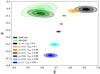 |
Fig. 8. 1-, 2- and 3-sigma contours of the emcee regressions in the slope-normalization ( |


Figure 8 shows that models reproducing the observed slope, namely the ones with higher μ (as in middle panel of Fig. 7), are also the ones that show weaker coronae (lower normalization  ) and overly extended L2 keV-emission (i.e. higher rpeak and r90, top panel of Fig. 7).
5.5. The 3D plane: LX vs LUV vs m
As shown by LR17, the LX − LUV relation for AGN is rather a three-dimensional problem, with the mass (or its proxy given by the full-width half-maximum of broad emission lines) playing a significant role as well. The observed LX − LUV − m plane from XMM-XXL can be fit by:
 (15)
(15)
and the mock LX − LUV − m from models with μ = 0, 0.5 and 1, respectively:
 (16)
(16)
The comparison in the 3D plane states that the exact dependency is not obtained by any of the models, with μ = 1 being the closest in qualitatively retrieving the coefficients for L3000 Å and m. We note that the mass is taken from the observations, thus this mismatch states that the luminosities in the model do not depend on the mass in the correct way.
5.6. The impact of the accretion efficiency
Throughout this work we adopted an efficiency ϵ0 = 0.057, typical of non-rotating black holes (e.g. Shapiro 2005), for simplicity. Nonetheless, a high spin seems to be preferred to model the blurred relativistic iron line, detected both in the local Universe (Nandra et al. 2007; Reynolds 2013) and up to z ∼ 4 (e.g. Baronchelli et al. 2018). Moreover, flux-limited samples are known to be biased in preferentially detecting high-spinning black holes (Brenneman et al. 2011; Vasudevan et al. 2016), simply because they are brighter than their non-rotating analogous (see Reynolds 2019).
Then, we tested the model using maximally-spinning black holes, with radiative efficiency 0.3 and ISCO down to r0 = 1.24rg (Thorne 1974). This has a major impact on the normalization axis of the LX − LUV. Everything else in the source being equal, in a spinning black hole matter can be accreted down to smaller distances with respect to their non-rotating companions, thus the accretion power in the system is much higher. As a matter of fact, changing the radiative efficiency has an impact on the numerical equation that regulates f(r): for the same m and ṁ and r > 3 the values of f is higher, and the transition radius between Prad- and Pgas-dominated regions moves at lower radii. This self-consistently affects the disk equations via the  factor (see Appendix A), hence the surface temperature is decreased at higher radii, where most of the disk emission at 3000 Å comes from. Then, the modeled ṁ value needed to match the observed L3000 Å is higher (see Sect. 4.2) and, consequently, L2 keV ∝ fQ+ is higher.
In Fig. 9 we show the model contours in the correlation slope-normalization plane computed for both low and high radiative efficiency, for μ = 0.4, 0.5 and 0.6 only.
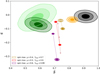 |
Fig. 9. Same as Fig. 8, with the addition of empty contours for μ = 0.4, 0.5 and 0.6 (color coded in the legend) obtained with maximally spinning black holes (i.e. with ϵ0 = 0.3 and r0 = 1.24rg). The dashed lines connect them to the non-spinning analogous realizations. Dark-red density spots represent the location of the center of different contours of the standard μ = 0.5 case, in which the only difference is the adoption of η (downward scattering component) varying among 0.4, 0.5 and 0.6, going from higher to lower |

Interestingly, maximally-spinning sources yield a better match with the data contours, in particular for the viscosity law μ = 0.5, with fmax = 0.9. For instance, Fig. 10 shows how the data and this high-spin model compare in the LX − LUV plane. We want to stress that using only a maximum spin for all sources is an extreme measure, but since the (unknown) observed spin distribution is likely dominated by high-spin values (Reynolds 2019), model contours of a more realistic diverse population of high-spinning sources would be closer to the high-efficiency ones in Fig. 9 rather than to the spin-zero case. We also note that, even if the modeled coronae would be somewhat weaker using a realistic spin distribution, with respect to the maximum-spin case, the model with μ = 0.5 can still be realized with a higher fmax = 0.99. Thus, we speculate that the new empty red contours in Fig. 9 consist in a fair approximation of a realistic high-spin population model. The tension with the observed LX − LUV would be significantly relaxed.
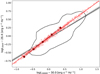 |
Fig. 10. LX − LUV relation for the high-spin model with μ = 0.5, α0 = 0.02 and fmax = 0.9 (empty red points, corresponding to the empty red contour in Fig. 9), with the red line showing best fit slope from emcee. The connected filled points (dark red) show the single-mass trend (log m = 8.7) for varying accretion rate (0.03, 0.07, 0.17, 0.42, 1). For a comparison, the black contour shows where the data lie in the plane, with the related best-fit slope (black line). |
5.7. The impact of the downward scattering component
The results shown in Fig. 6 are also degenerate with the assumptions on the value of the product η (1 − adisk), that is on the assumed downward component of the X-ray emission (η) and on the disk albedo. The adopted value of η = 0.55 is typical for anisotropic Comptonization in a plane-parallel corona (Haardt & Maraschi 1993), although it is unclear how much it would change in different geometries or prescriptions. In a patchy corona (Haardt et al. 1994) η would unlikely part significantly from the one in the slab case. The only major difference would rather involve the transmission or absorption by the corona of the radiation reflected by the disk. However, we conservatively excluded from the reference sample adopted in the observational test all the sources with a non-negligible reflection component detected (see Sect. 4.1), allowing us to avoid its complicated modeling. In an outflowing corona (e.g. Beloborodov 1999; Malzac et al. 2001), the ratio between the downward and the upward flux decreases with the bulk velocity of the corona (e.g. Janiuk et al. 2000). We tried to quantify possible offsets in the  -
- plane due to different values of η, ranging from 0.6 (slightly enhanced downward scattering) to 0.4 (reduced downward scattering, roughly approximating an outflowing corona with βbulk ≈ 0.1 − 0.2, e.g. Janiuk et al. 2000). We show this in Fig. 9 for the μ = 0.5 case, with dark-red density spots (η = 0.4, 0.5 and 0.6 from higher to lower
  , respectively). Changing the downward component by Δη ∼ 0.1 induces a significant offset of ≈0.1 dex in
  and a minor change in
  .
.
6. Discussion
The LX − LUV relation has been studied for decades (starting with the better-known αOX parameter, Tananbaum et al. 1979), its robustness used for bolometric estimates (e.g. Marconi et al. 2004; Hopkins et al. 2007; Lusso et al. 2010) and recently even for cosmology (Risaliti & Lusso 2015, 2019). Nonetheless, there is currently no solid and exhaustive physical explanation for it. In Sect. 3 we outlined the qualitative predictions of our model and in Sect. 5 we obtained that concordance with current data can be obtained with a modified viscosity prescription in the accretion flow (μ = 0.5), provided the spin of the sources is high. Here, we briefly discuss whether other competing analytic disk-corona models succeed or not and then we try to investigate the impact of the assumptions in our model on the results.
6.1. Comparison with other models
LR17 tried to explain this relation with a very simplified, but effective, toy-model. Most of their assumptions are in common with our work (see Sect. 6.2), although our treatment is more complete and physically motivated. The assumption of the MRI amplifying the magnetic field to a lesser extent in Prad-dominated regions (Blaes & Socrates 2001; Turner et al. 2002; M03) is taken to the extreme with a step function for the f-profile: all the accretion power is emitted by the disk in Prad-dominated regions (i.e. f(rrad)=0), whereas it is equally distributed between disk and corona in Pgas-dominated regions (i.e. f(rgas)=0.5). The resulting predicted slope and normalization of the LX − LUV are claimed to be consistent with the observations. The former can be confirmed by our analysis, as their f(r) step-function is nothing but an extremely damped f(r) beyond μ = 1, whose mock slope of the LX − LUV was the closest to the observed one. In the latter case, their match in normalization might be an involuntary artifact: with respect to the power transferred to the corona f, the observed luminosity is roughly halved if a downward scattering component is included (i.e. f(1 − η), with η ≈ 0.5). We verified this running our model with μ = 0 and α0 = 0.02, forcing f = 0 in the Prad-dominated region and fixing both f = 0.50 and f = 0.99 in Pgas-dominated radii. In Fig. 11 we show the related contours in the  plane along with our results of Fig. 8. This confirms that their step f-profile results in a slope consistent with the observed value, albeit producing overly weak coronae (too low normalization in the
  ). Hence, their toy-model does not reproduce the LX − LUV. Moreover, the X-ray emission from their toy-model inevitably peaks at the transition radius between Prad- and Pgas-dominated regions. Indeed, their model with fgas = 0.99 yields
  and
and  (i.e. produces extremely extended coronae).
Kubota & Done (2018) coupled an outer standard disk with an inner warm Componising region, that produces the soft X-ray excess, and an innermost hot corona for the hard X-ray continuum. Their model fits remarkably well the broadband continua of three sources spanning a wide range of accretion rates. They also claim to reproduce the observed LX − LUV, using both the regression line and data points from LR17, although only displaying all the possible sources modeled within a grid of m = 106 − 1010 and ṁ = 0.03 − 1 (their Figs. 7 and 8). Nonetheless, first-order normalization matches, even with m and ṁ spanning within typical values, can be misleading. A more conclusive test would be, as we do, to match mock and data sources one by one.
6.2. Further assumptions and theoretical uncertainties
Only models with μ ≲ 0.4 are able to reproduce the observed normalization within the range of possible fmax values, whereas for μ ≳ 0.5 they are off by ≳0.1 − 0.2 dex along the normalization. In Sects. 5.6 and 5.7 we showed how a higher accretion efficiency and/or a different downward scattering component may affect our results in the slope-normalization plane. Their impact would be significant and can possibly ease the tension between data and models: high-spin black holes and/or moderately outflowing coronae would be consistent with the observations. We now try to investigate some other simplifications of our model, likely to have a minor or less quantifiable effect on our conclusions.
6.2.1. Soft X-ray excess and thermal instability
The XMM-XXL L2 keV value was interpolated from the L2 − 10 keV fit in L16 after excluding sources with high reflection fraction (Sect. 4.1). The impact of the soft X-ray excess component can be considered negligible in that energy range, thus data points in the LX − LUV are likely not contaminated. However, our models do not include a soft X-ray excess generation mechanism, the monochromatic L2 keV being extracted from a power-law spectrum within 0.1 − 100 keV. If a significant fraction of the power dissipated in the corona is actually used by a different mechanism producing the observed soft-excess, namely from a warm corona (e.g. Petrucci et al. 2018; Kubota & Done 2018; Middei et al. 2019), the mock L2 keV would be overestimated to an unclear extent. Nonetheless, if the soft X-ray excess is produced by blurred relativistic reflection (e.g. Crummy et al. 2006; Garcia et al. 2019), the influence of this component on our analysis would have been excluded with our selection criteria (Sect. 4.1).
In Sect. 2, we briefly addressed the disk-instability problem (see Fig. 1, top panel) and despite the local stabilizing effect of the iron bump in the opacities, disks with μ = 0 (e.g., SS73) and 0.5 (e.g., M03) are globally unstable in Prad-dominated regions. An intriguing question may be whether the unstable regions in the disk are responsible for generating the soft-excess, possibly within inhomogeneous flows (e.g. Merloni et al. 2006). As a matter of fact, the higher ṁ the wider the region where Prad dominates and the higher the soft-excess strength (e.g. Boissay et al. 2016). Nonetheless, a more thorough investigation of this scenario is beyond the reach of this paper.
6.2.2. Magnetically-dominated disks
In our model the stress tensor is dominated by Maxwell stresses as confirmed by simulations (e.g., Hawley et al. 1995; Sano et al. 2004; Minoshima et al. 2015), although the magnetic pressure is bound to be only a fraction of the product  via α0 at the mid-plane. However, there are theories postulating disks that are Pmag-dominated also in the denser regions (e.g. Begelman & Silk 2017, and references therein) and not only in the upper layers (e.g. Miller & Stone 2000), possibly solving a few long-standing issues of the standard accretions disk theory (Dexter & Begelman 2019). Simulations indeed showed that Pmag can become an important competitor in supporting the disk vertically (Bai & Stone 2013; Salvesen et al. 2016), although heavily depending on the strength of the net vertical magnetic field, the origin of which is not fully understood, yet. If this imposed net vertical field is small (if β0 = Ptot/Pmag > > 1), the buoyant escape of the toroidal component, amplified by MRI, is faster than its creation and a disk-corona system consistent with our model is formed. However, the evidence of disks that are magnetically-dominated even at the mid-plane is supported by Jiang et al. (2019), that recently performed a global 3D radiation-MHD simulation of two sub-Eddingtion flows. The structure of their simulated disks is significantly different from the standard SS73 model and reaches a complexity that our simplified prescriptions are not able to grasp. On the other hand, these simulations could not produce spectra and luminosities, yet. We here rely on the assumption that the energetics of Pmag-dominated disks are not significantly different from standard thin disks at radii larger than ∼10rg (e.g., see Sdowski 2016).
6.2.3. Winds and outflows
In order to see if any known broad absorption line (BAL) quasars were present in our sample, we cross-matched the XMM-XXL catalog (L16; Menzel et al. 2016) with SDSS-DR12 (Pâris et al. 2017), that flagged 29580 BAL QSO after visual inspection. Only two sources among the 379 used in our analysis were flagged, although they were both assigned zero indexes in the common metrics used for a more quantitative measurement of the BAL properties (Pâris et al. 2017). Hence, our sample has no contaminations from known BALs, although we can investigate the possible impact of un-modeled wind-dominated objects on our work. For instance, Nomura et al. (2018) recently developed a disk model compensating for the mass-loss rates of UV-driven winds, while consistently adjusting the temperature and emission of the underlying disk. They referred to a future work for a more complete modeling of the inner radii and the hard X-ray emission, but the influence on L3000 Å values seems already significant, provided ṁ ≳ 0.5. Since winds appear to act only from moderate to Eddington ṁ, neglecting their presence would have an impact on the modeled LX − LUV slope. The wind carries away kinetic energy reducing the disk emission accordingly, thus for a given observed high L3000 Å, our no-wind model would underestimate ṁ for the possible outflowing sources contaminating our sample.
6.2.4. The larger-than-predicted disk argument
One of the most studied issues of the standard SS73 disk model is that observed sizes appear to be larger than expected at optical-UV wavelengths, using both microlensing effects (e.g. Morgan et al. 2010; Blackburne et al. 2011; Jiménez-Vicente et al. 2012) and flux variability lags across multiple bands in the so-called reprocessing scenario (e.g. Edelson et al. 2015; Fausnaugh et al. 2016, 2018; Jiang et al. 2017b; Cackett et al. 2018; McHardy et al. 2018), in which often a compact X-ray emitting region (e.g., a lamppost corona) irradiates the disk inducing light-travel lags in the UV-optical bands. However, even combining all these results discordant with the theoretical predictions is not trivial (Kokubo 2018), particularly if different techniques are used (see Moreno et al. 2018; Vio & Andreani 2018). What is more, there are also numerous studies finding consistency with the sizes predicted by the standard SS73 theory (e.g. McHardy et al. 2016; Mudd et al. 2018; Yu et al. 2018; Edelson et al. 2019; Homayouni et al. 2019), thus we do not consider necessary to use the larger-than-predicted argument to abandon all the standard prescriptions, yet.
6.2.5. No-torque inner boundary
For convenience, we adopted the no-torque condition with the stress vanishing at the inner edge. However, the presence of magnetic torques (Gammie 1999; Agol & Krolik 2000) would increase the disk effective temperature and the Q+ emissivity in the innermost radii (Agol & Krolik 2000; Dezen & Flores 2018) and, if applied to the disk only, it would cause instead a drop in the fraction f (Merloni & Fabian 2003). Without a proper MHD treatment, it is unclear how the modeled L2 keV ∝ fQ+ would be affected, and consequently the LX − LUV slope.
6.2.6. The vertical structure
Our model does not properly treat the vertical structure of the disk. The effective temperature is obtained from Teff ∝ Tmid/τ1/4, where τ = h ρ κ assumes constant ρ and κ along the scale-height. Even keeping the approximation of a constant ρ, κ should change self-consistently with the decrease in temperature. A more thorough modeling of the disk vertical structure in supermassive black holes was presented by Hubeny and collaborators, taking into account both scattering processes and free-free and bound-free opacities (Hubeny et al. 2000, 2001). Their model also share some of our limits (e.g., stationary disk, α-prescription, no-torque boundary, vertical support from thermal pressure only), validating the comparison. The overall SED has lower (higher) fluxes at low (high) frequencies with respect to standard calculations, with the most significant impact on the modeling of the soft-excess (Done et al. 2012). The computation of L3000 Å should be affected in a minor way, with a small overestimation on the order of a color correction (e.g. Done et al. 2012), that is either roughly constant or weakly depending on m and ṁ (e.g. Davis & El-Abd 2019). Our conclusions should not be significantly affected, although this would need to be improved for a proper SED modeling and time-lags predictions.
7. Conclusions
The gap between simulations and observations in AGN needs to be bridged and simplified, but motivated, analytic prescriptions still represent a powerful tool to explain the observed multi-wavelength scaling relations. For instance, the clear correlation observed between monochromatic logarithmic LX and LUV luminosities has been used for decades (in the shape of the more-known αOX parameter, Tananbaum et al. 1979) in many applications (even for cosmology, e.g. Risaliti & Lusso 2015, 2019). Despite this, a conclusive theoretical explanation for the observed correlation is still lacking. Being smaller than one, the observed slope indicates that, going from low- to high-accretion rate AGN, the X-ray emission increases less than the optical-UV emission. Any viable disk-corona model must be able to explain this.
In this work, we tested a self-consistent disk-corona model (Sect. 2, see also M03) against the LX − LUV relation. We were able to identify the possible mechanism regulating the disk-corona energetic interplay, in terms of viscosity prescriptions (e.g., μ = 0.5) that naturally lead to an X-ray emission increasing less than the disk emission going to higher accretion rates (see Sect. 3).
We also put forward a quantitative observational test (Sect. 4), using a reference sample of AGN (Sect. 4.1) observed both in the (rest-frame) UV and in X-rays: taking from each source the observationally determined m, ṁ and Γ we were able to model an analogous mock object (Sect. 4.2) producing a set of mock LX − LUV. This allowed us to reach a deep understanding of the physics driving the slope, normalization and scatter of the LX − LUV (see Sect. 5).
We find that if the black-hole population is assumed to be non-spinning, results from this test are inconclusive: the viscosity prescriptions reproducing the slope of the observed LX − LUV relation, also produce overly weak coronae. Interestingly enough, the tension between the strength of the observed and modeled X-ray emission (i.e. in the normalization of the LX − LUV) can be significantly relaxed adopting a more realistic high-spinning black-hole population and/or with moderately-outflowing coronae. We tested the former case adopting the efficiency (and the inner orbit) of maximally-spinning black holes, in which matter is able to accrete further into the potential well, resulting in a much higher accretion power and, consequently, in much stronger coronae (Sect. 5.6). Moreover, if the spin is high the X-ray emission profile peaks closer to the black hole, in even better agreement with X-ray reverberation and microlensing studies (Mosquera et al. 2013; Reis & Miller 2013; Wilkins et al. 2016). In particular, the disk-corona model testing maximally-spinning black holes with μ = 0.5 (i.e. magnetic stress proportional to the geometric mean of Pgas and Ptot, e.g. see M03), fmax = 0.9, α0 = 0.02 (see Table 1) provides the best match with the observations (Fig. 10), although the modeled slope is still somewhat larger than the observed one (Fig. 9). Going beyond this type of exercises, only 3D global radiation-MHD simulations will be able to better disclose the disk-corona physics (e.g. Jiang et al. 2017a, 2019), provided a clearer way of approaching the observations will be reached.
We will refer to other data throughout the paper and possible discrepancies in luminosities due to different cosmological parameters may occur. Nonetheless, we verified that the biggest difference in luminosity values (∼0.01 dex) is obtained assuming a Planck with respect to a WMAP release, while using different releases of the same instrument will have a negligible impact (≲0.005 dex).
R is the ratio of the normalization of the reflection component with respect to the power-law component.
The distributions of mock ṁ are very similar across the models, with median values (and related 16th and 84th percentiles) of  ,
,  and
and  for μ = 0, 0.5 and 1, respectively. The tails include Eddington or even super-Eddington sources. We note that the uncertainty on the modeled ṁ, propagated through the ones in the observations, is as large as ≈0.65 dex.
XMM-XXL luminosities were obtained in L16 including a Balmer continuum component in the fit (refer to Shen & Liu 2012), although for the RM-QSO this component was switched off (Shen et al. 2019). For consistency, a rigid shift of −0.12 dex was applied to the RM-QSO L3000 Å (Shen & Liu 2012) for obtaining the contours displayed in Fig. 8.
Acknowledgments
We thank the referee for his/her helpful comments. We thank Teng Liu for kindly providing the optical spectral slopes obtained in (Liu et al. 2018). We are also grateful to Torben Simm for the RM-QSO data and to Elisabeta Lusso and Guido Risaliti for making available to us the data of LR17. RA thanks Damien Coffey, Jacob Ider Chitham and Linda Baronchelli for insightful discussions. We acknowledge the use of the matplotlib package (Hunter 2007).
References
- Agol, E., & Krolik, J. H. 2000, ApJ, 528, 161 [NASA ADS] [CrossRef] [Google Scholar]
- Antonucci, R. 2015, ArXiv e-prints [arXiv:1501.02001] [Google Scholar]
- Bai, X.-N., & Stone, J. M. 2013, ApJ, 767, 30 [NASA ADS] [CrossRef] [Google Scholar]
- Balbus, S. A., & Hawley, J. F. 1991, ApJ, 376, 214 [NASA ADS] [CrossRef] [Google Scholar]
- Balbus, S. A., & Hawley, J. F. 1992, ApJ, 400, 610 [CrossRef] [Google Scholar]
- Baronchelli, L., Nandra, K., & Buchner, J. 2018, MNRAS, 480, 2377 [NASA ADS] [Google Scholar]
- Begelman, M. C., & Silk, J. 2017, MNRAS, 464, 2311 [NASA ADS] [CrossRef] [Google Scholar]
- Beloborodov, A. M. 1999, in High Energy Processes in Accreting Black Holes, eds. J. Poutanen, & R. Svensson, ASP Conf. Ser., 161, 295 [NASA ADS] [Google Scholar]
- Beloborodov, A. M. 2017, ApJ, 850, 141 [NASA ADS] [CrossRef] [Google Scholar]
- Blackburne, J. A., Pooley, D., Rappaport, S., & Schechter, P. L. 2011, ApJ, 729, 34 [NASA ADS] [CrossRef] [Google Scholar]
- Blackman, E. G., & Pessah, M. E. 2009, ApJ, 704, L113 [NASA ADS] [CrossRef] [Google Scholar]
- Blaes, O. 2007, ASP Conf. Ser., 373, 75 [NASA ADS] [Google Scholar]
- Blaes, O. 2014, Space Sci. Rev., 183, 21 [NASA ADS] [CrossRef] [Google Scholar]
- Blaes, O., & Socrates, A. 2001, ApJ, 553, 987 [NASA ADS] [CrossRef] [Google Scholar]
- Boissay, R., Ricci, C., & Paltani, S. 2016, A&A, 588, A70 [NASA ADS] [CrossRef] [EDP Sciences] [Google Scholar]
- Brenneman, L. W., Reynolds, C. S., Nowak, M. A., et al. 2011, ApJ, 736, 103 [NASA ADS] [CrossRef] [Google Scholar]
- Buchner, J., Georgakakis, A., Nandra, K., et al. 2014, A&A, 564, A125 [NASA ADS] [CrossRef] [EDP Sciences] [Google Scholar]
- Burm, H. 1985, A&A, 143, 389 [NASA ADS] [Google Scholar]
- Cackett, E. M., Chiang, C.-Y., McHardy, I., et al. 2018, ApJ, 857, 53 [NASA ADS] [CrossRef] [Google Scholar]
- Cao, X. 2009, MNRAS, 394, 207 [NASA ADS] [CrossRef] [Google Scholar]
- Capellupo, D. M., Netzer, H., Lira, P., Trakhtenbrot, B., & Mejía-Restrepo, J. 2015, MNRAS, 446, 3427 [NASA ADS] [CrossRef] [Google Scholar]
- Capellupo, D. M., Netzer, H., Lira, P., Trakhtenbrot, B., & Mejía-Restrepo, J. 2016, MNRAS, 460, 212 [NASA ADS] [CrossRef] [Google Scholar]
- Chandrasekhar, S. 1960, Proc. Natl. Acad. Sci., 46, 253 [NASA ADS] [CrossRef] [Google Scholar]
- Chiaraluce, E., Vagnetti, F., Tombesi, F., & Paolillo, M. 2018, A&A, 619, A95 [NASA ADS] [CrossRef] [EDP Sciences] [Google Scholar]
- Crummy, J., Fabian, A. C., Gallo, L., & Ross, R. R. 2006, MNRAS, 365, 1067 [NASA ADS] [CrossRef] [Google Scholar]
- Czerny, B., Du, P., Wang, J.-M., & Karas, V. 2016, ApJ, 832, 15 [NASA ADS] [CrossRef] [Google Scholar]
- D’Agostini, G. 2003, Bayesian Reasoning in Data Analysis: A Critical Introduction (New Jersey, USA: World Scientific) [CrossRef] [Google Scholar]
- D’Agostini, G. 2005, ArXiv e-prints [arXiv:physics/0511182] [Google Scholar]
- Davis, S. W., & El-Abd, S. 2019, ApJ, 874, 23 [NASA ADS] [CrossRef] [Google Scholar]
- Davis, S. W., & Laor, A. 2011, ApJ, 728, 98 [CrossRef] [Google Scholar]
- Della Ceca, R., Caccianiga, A., Severgnini, P., et al. 2008, A&A, 487, 119 [NASA ADS] [CrossRef] [EDP Sciences] [Google Scholar]
- De Marco, B., Ponti, G., Cappi, M., et al. 2013, MNRAS, 431, 2441 [NASA ADS] [CrossRef] [Google Scholar]
- Dexter, J., & Begelman, M. C. 2019, MNRAS, 483, L17 [NASA ADS] [CrossRef] [Google Scholar]
- Dezen, T., & Flores, B. 2018, ApJ, 861, 18 [NASA ADS] [CrossRef] [Google Scholar]
- Di Matteo, T. 1998, MNRAS, 299, L15 [NASA ADS] [CrossRef] [Google Scholar]
- Done, C., Davis, S. W., Jin, C., Blaes, O., & Ward, M. 2012, MNRAS, 420, 1848 [NASA ADS] [CrossRef] [Google Scholar]
- Edelson, R., Gelbord, J. M., Horne, K., et al. 2015, ApJ, 806, 129 [NASA ADS] [CrossRef] [Google Scholar]
- Edelson, R., Gelbord, J., Cackett, E., et al. 2019, ApJ, 870, 123 [NASA ADS] [CrossRef] [Google Scholar]
- Elvis, M., Maccacaro, T., Wilson, A. S., et al. 1978, MNRAS, 183, 129 [NASA ADS] [Google Scholar]
- Fabian, A. C., Zoghbi, A., Ross, R. R., et al. 2009, Nature, 459, 540 [NASA ADS] [CrossRef] [PubMed] [Google Scholar]
- Fabian, A. C., Alston, W. N., Cackett, E. M., et al. 2017, Astron. Nachr., 338, 269 [NASA ADS] [CrossRef] [Google Scholar]
- Fausnaugh, M. M., Denney, K. D., Barth, A. J., et al. 2016, ApJ, 821, 56 [NASA ADS] [CrossRef] [Google Scholar]
- Fausnaugh, M. M., Starkey, D. A., Horne, K., et al. 2018, ApJ, 854, 107 [NASA ADS] [CrossRef] [Google Scholar]
- Foreman-Mackey, D., Hogg, D. W., Lang, D., & Goodman, J. 2013, PASP, 125, 306 [CrossRef] [Google Scholar]
- Galeev, A. A., Rosner, R., & Vaiana, G. S. 1979, ApJ, 229, 318 [NASA ADS] [CrossRef] [Google Scholar]
- Gammie, C. F. 1999, ApJ, 522, L57 [NASA ADS] [CrossRef] [Google Scholar]
- Garcia, J. A., Kara, E., Walton, D., et al. 2019, ApJ, 871, 88 [NASA ADS] [CrossRef] [Google Scholar]
- Grzȩdzielski, M., Janiuk, A., Czerny, B., & Wu, Q. 2017a, A&A, 603, A110 [NASA ADS] [CrossRef] [EDP Sciences] [Google Scholar]
- Grzȩdzielski, M., Janiuk, A., & Czerny, B. 2017b, ApJ, 845, 20 [NASA ADS] [CrossRef] [Google Scholar]
- Haardt, F., & Maraschi, L. 1991, ApJ, 380, L51 [NASA ADS] [CrossRef] [Google Scholar]
- Haardt, F., & Maraschi, L. 1993, ApJ, 413, 507 [NASA ADS] [CrossRef] [MathSciNet] [Google Scholar]
- Haardt, F., Maraschi, L., & Ghisellini, G. 1994, ApJ, 432, L95 [NASA ADS] [CrossRef] [Google Scholar]
- Hawley, J. F., & Balbus, S. A. 1991, ApJ, 376, 223 [NASA ADS] [CrossRef] [Google Scholar]
- Hawley, J. F., & Balbus, S. A. 1992, ApJ, 400, 595 [NASA ADS] [CrossRef] [Google Scholar]
- Hawley, J. F., Gammie, C. F., & Balbus, S. A. 1995, ApJ, 440, 742 [NASA ADS] [CrossRef] [Google Scholar]
- Homayouni, Y., Trump, J. R., Grier, C. J., et al. 2019, ApJ, 880, 126 [NASA ADS] [CrossRef] [Google Scholar]
- Hopkins, P. F., Richards, G. T., & Hernquist, L. 2007, ApJ, 654, 731 [NASA ADS] [CrossRef] [Google Scholar]
- Hoshi, R. 1985, in Galactic and Extra-Galactic Compact X-ray Sources, eds. Y. Tabaka, & W. H. G. Lewin, 143 [Google Scholar]
- Hubeny, I., Agol, E., Blaes, O., & Krolik, J. H. 2000, ApJ, 533, 710 [NASA ADS] [CrossRef] [Google Scholar]
- Hubeny, I., Blaes, O., Krolik, J. H., & Agol, E. 2001, ApJ, 559, 680 [NASA ADS] [CrossRef] [Google Scholar]
- Hunter, J. D. 2007, Comput. Sci. Eng., 9, 90 [NASA ADS] [CrossRef] [Google Scholar]
- Ichimaru, S. 1977, ApJ, 214, 840 [NASA ADS] [CrossRef] [Google Scholar]
- Janiuk, A., Czerny, B., & Życki, P. T. 2000, MNRAS, 318, 180 [NASA ADS] [CrossRef] [Google Scholar]
- Jansen, F., Lumb, D., Altieri, B., et al. 2001, A&A, 365, L1 [NASA ADS] [CrossRef] [EDP Sciences] [Google Scholar]
- Jiang, Y.-F., Stone, J. M., & Davis, S. W. 2014, ApJ, 784, 169 [NASA ADS] [CrossRef] [Google Scholar]
- Jiang, Y.-F., Davis, S. W., & Stone, J. M. 2016, ApJ, 827, 10 [NASA ADS] [CrossRef] [Google Scholar]
- Jiang, Y. F., Stone, J., & Davis, S. W. 2017a, ArXiv e-prints [arXiv:1709.02845] [Google Scholar]
- Jiang, Y.-F., Green, P. J., Greene, J. E., et al. 2017b, ApJ, 836, 186 [NASA ADS] [CrossRef] [Google Scholar]
- Jiang, Y. F., Blaes, O., Stone, J., & Davis, S. W. 2019, ApJ, submitted [arXiv:1904.01674] [Google Scholar]
- Jiménez-Vicente, J., Mediavilla, E., Muñoz, J. A., & Kochanek, C. S. 2012, ApJ, 751, 106 [NASA ADS] [CrossRef] [Google Scholar]
- Jin, C., Ward, M., & Done, C. 2012, MNRAS, 422, 3268 [NASA ADS] [CrossRef] [Google Scholar]
- Kadowaki, L. H. S., de Gouveia Dal Pino, E. M., & Stone, J. M. 2018, ApJ, 864, 52 [NASA ADS] [CrossRef] [Google Scholar]
- Kelly, B. C., Bechtold, J., Trump, J. R., Vestergaard, M., & Siemiginowska, A. 2008, ApJS, 176, 355 [NASA ADS] [CrossRef] [Google Scholar]
- Kilerci Eser, E., & Vestergaard, M. 2018, MNRAS, 474, 1590 [NASA ADS] [CrossRef] [Google Scholar]
- Kishimoto, M., Antonucci, R., Blaes, O., et al. 2008, Nature, 454, 492 [NASA ADS] [CrossRef] [PubMed] [Google Scholar]
- Kokubo, M. 2018, PASJ, 70, 97 [NASA ADS] [CrossRef] [Google Scholar]
- Koratkar, A., & Blaes, O. 1999, PASP, 111, 1 [NASA ADS] [CrossRef] [Google Scholar]
- Krawczyk, C. M., Richards, G. T., Mehta, S. S., et al. 2013, ApJS, 206, 4 [NASA ADS] [CrossRef] [Google Scholar]
- Kubota, A., & Done, C. 2018, MNRAS, 480, 1247 [NASA ADS] [CrossRef] [Google Scholar]
- Liang, E. P. T., & Price, R. H. 1977, ApJ, 218, 247 [NASA ADS] [CrossRef] [Google Scholar]
- Lightman, A. P., & Eardley, D. M. 1974, ApJ, 187, L1 [NASA ADS] [CrossRef] [Google Scholar]
- Lightman, A. P., & White, T. R. 1988, ApJ, 335, 57 [NASA ADS] [CrossRef] [Google Scholar]
- Liu, J.-Y., & Liu, B.-F. 2009, Res. Astron. Astrophys., 9, 966 [NASA ADS] [CrossRef] [Google Scholar]
- Liu, B. F., Mineshige, S., & Shibata, K. 2002, ApJ, 572, L173 [NASA ADS] [CrossRef] [Google Scholar]
- Liu, J. Y., Liu, B. F., Qiao, E. L., & Mineshige, S. 2012, ApJ, 754, 81 [NASA ADS] [CrossRef] [Google Scholar]
- Liu, J. Y., Qiao, E. L., & Liu, B. F. 2016a, ApJ, 833, 35 [NASA ADS] [CrossRef] [Google Scholar]
- Liu, Z., Merloni, A., Georgakakis, A., et al. 2016b, MNRAS, 459, 1602 [NASA ADS] [CrossRef] [Google Scholar]
- Liu, T., Merloni, A., Wang, J.-X., et al. 2018, MNRAS, 479, 5022 [NASA ADS] [CrossRef] [Google Scholar]
- Lusso, E. 2019, Astron. Nachr., 340, 267 [NASA ADS] [CrossRef] [Google Scholar]
- Lusso, E., & Risaliti, G. 2016, ApJ, 819, 154 [NASA ADS] [CrossRef] [Google Scholar]
- Lusso, E., & Risaliti, G. 2017, A&A, 602, A79 [NASA ADS] [CrossRef] [EDP Sciences] [Google Scholar]
- Lusso, E., Comastri, A., Vignali, C., et al. 2010, A&A, 512, A34 [NASA ADS] [CrossRef] [EDP Sciences] [Google Scholar]
- Lusso, E., Comastri, A., Simmons, B. D., et al. 2012, MNRAS, 425, 623 [NASA ADS] [CrossRef] [Google Scholar]
- Malzac, J., Beloborodov, A. M., & Poutanen, J. 2001, MNRAS, 326, 417 [NASA ADS] [CrossRef] [Google Scholar]
- Marconi, A., Risaliti, G., Gilli, R., et al. 2004, MNRAS, 351, 169 [NASA ADS] [CrossRef] [Google Scholar]
- McHardy, I. M. 1989, in Two Topics in X-Ray Astronomy, Volume 1: X Ray Binaries. Volume 2: AGN and the X Ray Background, eds. J. Hunt, & B. Battrick, ESA Spec. Publ., 296 [Google Scholar]
- McHardy, I. M., Connolly, S. D., Peterson, B. M., et al. 2016, Astron. Nachr., 337, 500 [NASA ADS] [CrossRef] [Google Scholar]
- McHardy, I. M., Connolly, S. D., Horne, K., et al. 2018, MNRAS, 480, 2881 [NASA ADS] [CrossRef] [Google Scholar]
- Menzel, M.-L., Merloni, A., Georgakakis, A., et al. 2016, MNRAS, 457, 110 [NASA ADS] [CrossRef] [Google Scholar]
- Merloni, A. 2003, MNRAS, 341, 1051 [NASA ADS] [CrossRef] [Google Scholar]
- Merloni, A., & Fabian, A. C. 2002, MNRAS, 332, 165 [NASA ADS] [CrossRef] [Google Scholar]
- Merloni, A., & Fabian, A. C. 2003, MNRAS, 342, 951 [NASA ADS] [CrossRef] [Google Scholar]
- Merloni, A., & Nayakshin, S. 2006, MNRAS, 372, 728 [NASA ADS] [CrossRef] [Google Scholar]
- Merloni, A., Malzac, J., Fabian, A. C., & Ross, R. R. 2006, MNRAS, 370, 1699 [NASA ADS] [CrossRef] [Google Scholar]
- Merloni, A., Bongiorno, A., Brusa, M., et al. 2014, MNRAS, 437, 3550 [NASA ADS] [CrossRef] [Google Scholar]
- Meyer, F., & Meyer-Hofmeister, E. 1982, A&A, 106, 34 [NASA ADS] [Google Scholar]
- Middei, R., Bianchi, S., Petrucci, P.-O., et al. 2019, MNRAS, 483, 4695 [NASA ADS] [CrossRef] [Google Scholar]
- Miller, K. A., & Stone, J. M. 2000, ApJ, 534, 398 [NASA ADS] [CrossRef] [Google Scholar]
- Minoshima, T., Hirose, S., & Sano, T. 2015, ApJ, 808, 54 [NASA ADS] [CrossRef] [Google Scholar]
- Moreno, J., Vogeley, M. S., & Richards, G. T. 2018, PASP, submitted [arXiv:1811.00154] [Google Scholar]
- Morgan, C. W., Kochanek, C. S., Morgan, N. D., & Falco, E. E. 2010, ApJ, 712, 1129 [NASA ADS] [CrossRef] [Google Scholar]
- Mosquera, A. M., Kochanek, C. S., Chen, B., et al. 2013, ApJ, 769, 53 [NASA ADS] [CrossRef] [Google Scholar]
- Mudd, D., Martini, P., Zu, Y., et al. 2018, ApJ, 862, 123 [NASA ADS] [CrossRef] [Google Scholar]
- Nandra, K., Pounds, K. A., Stewart, G. C., et al. 1991, MNRAS, 248, 760 [NASA ADS] [CrossRef] [Google Scholar]
- Nandra, K., O’Neill, P. M., George, I. M., & Reeves, J. N. 2007, MNRAS, 382, 194 [NASA ADS] [CrossRef] [Google Scholar]
- Nomura, M., Ohsuga, K., & Done, C. 2018, MNRAS, submitted [arXiv:1811.01966] [Google Scholar]
- Pâris, I., Petitjean, P., Ross, N. P., et al. 2017, A&A, 597, A79 [NASA ADS] [CrossRef] [EDP Sciences] [Google Scholar]
- Petrucci, P.-O., Ursini, F., De Rosa, A., et al. 2018, A&A, 611, A59 [NASA ADS] [CrossRef] [EDP Sciences] [Google Scholar]
- Pierre, M., Pacaud, F., Adami, C., et al. 2016, A&A, 592, A1 [NASA ADS] [CrossRef] [EDP Sciences] [Google Scholar]
- Pounds, K. A., Nandra, K., Stewart, G. C., George, I. M., & Fabian, A. C. 1990, Nature, 344, 132 [NASA ADS] [CrossRef] [Google Scholar]
- Pringle, J. E. 1976, MNRAS, 177, 65 [NASA ADS] [Google Scholar]
- Pringle, J. E. 1981, ARA&A, 19, 137 [NASA ADS] [CrossRef] [Google Scholar]
- Reis, R. C., & Miller, J. M. 2013, ApJ, 769, L7 [Google Scholar]
- Reynolds, C. S. 2013, Classical and Quantum Gravity, 30, 244004 [NASA ADS] [CrossRef] [Google Scholar]
- Reynolds, C. S. 2019, Nat. Astron., 3, 41 [NASA ADS] [CrossRef] [Google Scholar]
- Richards, G. T., Lacy, M., Storrie-Lombardi, L. J., et al. 2006, ApJS, 166, 470 [NASA ADS] [CrossRef] [Google Scholar]
- Ripperda, B., Porth, O., Sironi, L., & Keppens, R. 2019, MNRAS, 485, 299 [NASA ADS] [CrossRef] [Google Scholar]
- Risaliti, G., & Lusso, E. 2015, ApJ, 815, 33 [NASA ADS] [CrossRef] [Google Scholar]
- Risaliti, G., & Lusso, E. 2019, Nat. Astron., 3, 272 [NASA ADS] [CrossRef] [Google Scholar]
- Ross, J., Latter, H. N., & Guilet, J. 2016, MNRAS, 455, 526 [NASA ADS] [CrossRef] [Google Scholar]
- Runnoe, J. C., Brotherton, M. S., & Shang, Z. 2012, MNRAS, 422, 478 [NASA ADS] [CrossRef] [Google Scholar]
- Sakimoto, P. J., & Coroniti, F. V. 1981, ApJ, 247, 19 [NASA ADS] [CrossRef] [Google Scholar]
- Salvesen, G., Simon, J. B., Armitage, P. J., & Begelman, M. C. 2016, MNRAS, 457, 857 [NASA ADS] [CrossRef] [Google Scholar]
- Sano, T., Inutsuka, S.-I., Turner, N. J., & Stone, J. M. 2004, ApJ, 605, 321 [NASA ADS] [CrossRef] [Google Scholar]
- Sdowski, A. 2016, MNRAS, 459, 4397 [NASA ADS] [CrossRef] [Google Scholar]
- Schnittman, J. D., Krolik, J. H., & Noble, S. C. 2013, ApJ, 769, 156 [NASA ADS] [CrossRef] [Google Scholar]
- Seaton, M. J. 1995, The Opacity Project (Bristol, UK: Institute of Physics Pub.) [Google Scholar]
- Seaton, M. J., Yan, Y., Mihalas, D., & Pradhan, A. K. 1994, MNRAS, 266, 805 [NASA ADS] [CrossRef] [Google Scholar]
- Shadmehri, M., Khajenabi, F., Dib, S., & Inutsuka, S.-I. 2018, MNRAS, 481, 5170 [NASA ADS] [CrossRef] [Google Scholar]
- Shakura, N. I., & Sunyaev, R. A. 1973, A&A, 24, 337 [NASA ADS] [Google Scholar]
- Shakura, N. I., & Sunyaev, R. A. 1976, MNRAS, 175, 613 [NASA ADS] [CrossRef] [Google Scholar]
- Shapiro, S. L. 2005, ApJ, 620, 59 [NASA ADS] [CrossRef] [Google Scholar]
- Shen, Y. 2013, Bull. Astron. Soc. India, 41, 61 [NASA ADS] [Google Scholar]
- Shen, Y., & Liu, X. 2012, ApJ, 753, 125 [NASA ADS] [CrossRef] [Google Scholar]
- Shen, Y., Greene, J. E., Strauss, M. A., Richards, G. T., & Schneider, D. P. 2008, ApJ, 680, 169 [NASA ADS] [CrossRef] [Google Scholar]
- Shen, Y., Hall, P. B., Horne, K., et al. 2019, ApJS, 241, 34 [NASA ADS] [CrossRef] [Google Scholar]
- Slone, O., & Netzer, H. 2012, MNRAS, 426, 656 [NASA ADS] [CrossRef] [Google Scholar]
- Steffen, A. T., Strateva, I., Brandt, W. N., et al. 2006, AJ, 131, 2826 [NASA ADS] [CrossRef] [Google Scholar]
- Stella, L., & Rosner, R. 1984, ApJ, 277, 312 [NASA ADS] [CrossRef] [Google Scholar]
- Stern, B. E., Poutanen, J., Svensson, R., Sikora, M., & Begelman, M. C. 1995, ApJ, 449, L13 [NASA ADS] [CrossRef] [Google Scholar]
- Strateva, I. V., Brandt, W. N., Schneider, D. P., Vanden Berk, D. G., & Vignali, C. 2005, AJ, 130, 387 [NASA ADS] [CrossRef] [Google Scholar]
- Strüder, L., Briel, U., Dennerl, K., et al. 2001, A&A, 365, L18 [NASA ADS] [CrossRef] [EDP Sciences] [Google Scholar]
- Svensson, R., & Zdziarski, A. A. 1994, ApJ, 436, 599 [NASA ADS] [CrossRef] [Google Scholar]
- Szuszkiewicz, E. 1990, MNRAS, 244, 377 [NASA ADS] [Google Scholar]
- Taam, R. E., & Lin, D. N. C. 1984, ApJ, 287, 761 [NASA ADS] [CrossRef] [Google Scholar]
- Tanaka, Y., Nandra, K., Fabian, A. C., et al. 1995, Nature, 375, 659 [NASA ADS] [CrossRef] [Google Scholar]
- Tananbaum, H., Avni, Y., Branduardi, G., et al. 1979, ApJ, 234, L9 [NASA ADS] [CrossRef] [Google Scholar]
- Thorne, K. S. 1974, ApJ, 191, 507 [Google Scholar]
- Turner, T. J., & Pounds, K. A. 1989, MNRAS, 240, 833 [NASA ADS] [CrossRef] [Google Scholar]
- Turner, M. J. L., Abbey, A., Arnaud, M., et al. 2001, A&A, 365, L27 [NASA ADS] [CrossRef] [EDP Sciences] [Google Scholar]
- Turner, N. J., Stone, J. M., & Sano, T. 2002, ApJ, 566, 148 [NASA ADS] [CrossRef] [Google Scholar]
- Uttley, P., Cackett, E. M., Fabian, A. C., Kara, E., & Wilkins, D. R. 2014, A&ARv, 22, 72 [NASA ADS] [CrossRef] [EDP Sciences] [Google Scholar]
- Uzdensky, D. A. 2013, ApJ, 775, 103 [NASA ADS] [CrossRef] [Google Scholar]
- Uzdensky, D. A. 2016, Astrophys. Space Sci. Lib., 427, 473 [NASA ADS] [CrossRef] [Google Scholar]
- Uzdensky, D. A., & Goodman, J. 2008, ApJ, 682, 608 [NASA ADS] [CrossRef] [Google Scholar]
- Vagnetti, F., Antonucci, M., & Trevese, D. 2013, A&A, 550, A71 [NASA ADS] [CrossRef] [EDP Sciences] [Google Scholar]
- Vasudevan, R. V., & Fabian, A. C. 2007, MNRAS, 381, 1235 [NASA ADS] [CrossRef] [Google Scholar]
- Vasudevan, R. V., & Fabian, A. C. 2009, MNRAS, 392, 1124 [NASA ADS] [CrossRef] [Google Scholar]
- Vasudevan, R. V., Fabian, A. C., Reynolds, C. S., et al. 2016, MNRAS, 458, 2012 [NASA ADS] [CrossRef] [Google Scholar]
- Vignali, C., Brandt, W. N., & Schneider, D. P. 2003, AJ, 125, 433 [NASA ADS] [CrossRef] [Google Scholar]
- Vio, R., & Andreani, P. 2018, ArXiv e-prints [arXiv:1812.03995] [Google Scholar]
- Wang, J.-M., Watarai, K.-Y., & Mineshige, S. 2004, ApJ, 607, L107 [NASA ADS] [CrossRef] [Google Scholar]
- Wang, C., Yu, L.-M., Bian, W.-H., & Zhao, B.-X. 2019, MNRAS, 487, 2463 [NASA ADS] [CrossRef] [Google Scholar]
- Werner, G. R., Philippov, A. A., & Uzdensky, D. A. 2019, MNRAS, 482, L60 [NASA ADS] [CrossRef] [Google Scholar]
- Wilkins, D. R., Cackett, E. M., Fabian, A. C., & Reynolds, C. S. 2016, MNRAS, 458, 200 [NASA ADS] [CrossRef] [Google Scholar]
- Williams, O. R., Turner, M. J. L., Stewart, G. C., et al. 1992, ApJ, 389, 157 [NASA ADS] [CrossRef] [Google Scholar]
- You, B., Cao, X., & Yuan, Y.-F. 2012, ApJ, 761, 109 [NASA ADS] [CrossRef] [Google Scholar]
- Young, M., Elvis, M., & Risaliti, G. 2009, ApJS, 183, 17 [NASA ADS] [CrossRef] [Google Scholar]
- Young, M., Elvis, M., & Risaliti, G. 2010, ApJ, 708, 1388 [NASA ADS] [CrossRef] [Google Scholar]
- Yu, Z., Martini, P., Davis, T. M., et al. 2018, ArXiv e-prints [arXiv:1811.03638] [Google Scholar]
Appendix A: Disc-corona equations
We report the equations for h, mid-plane ρ (g cm−3), P (dyn cm−2), T (K, at the mid-plane) and the closure equation for f. In the radiation pressure dominated regime:
![Mathematical equation: $$ \begin{aligned}&\rho =\rho _{\rm const}\, k_0^{-\frac{4}{\mu +4}}[\alpha _0m]^{-\frac{4}{\mu +4}} [\dot{m}J(r)]^{\frac{2(3\mu -4)}{\mu +4}} r^{\frac{3(2-3\mu )}{\mu +4}} (1-\tilde{f})^{\frac{6(\mu -2)}{\mu +4}} \nonumber \\&T=T_{\rm const}\,k_0^{-\frac{1}{\mu +4}}[\alpha _0m]^{-\frac{1}{\mu +4}} [\dot{m}J(r)]^{\frac{2\mu }{\mu +4}} r^{\frac{3(2\mu ^2-3\mu -2)}{2(2-\mu )(\mu +4)}} (1-\tilde{f})^{\frac{2\mu -1}{\mu +4}} \nonumber \\&h=9.14\,\dot{m}J(r)(1-\tilde{f}) \nonumber \\&P=P_{\rm const}\,k_0^{-\frac{4}{\mu +4}}[\alpha _0m]^{-\frac{4}{\mu +4}} [\dot{m}J(r)]^{\frac{8\mu }{\mu +4}} r^{\frac{6(2\mu ^2-3\mu -2)}{(2-\mu )(\mu +4)}} (1-\tilde{f})^{\frac{4(2\mu -1)}{\mu +4}} \nonumber \\&\frac{(2\alpha _0)^{1/\mu }-k_1^{2/\mu }f^{2/\mu }}{k_1^{2/\mu }f^{2/\mu }}= \tilde{C}\,k_0^{\frac{1}{\mu +4}}[\alpha _0m]^{\frac{1}{\mu +4}} [\dot{m}J(r)]^{\frac{8}{\mu +4}} r^{-\frac{21}{2(\mu +4)}} (1-\tilde{f})^{\frac{9}{\mu +4}} \end{aligned} $$](/articles/aa/full_html/2019/08/aa35874-19/aa35874-19-eq56.gif) (A.1)
(A.1)
where k0 is the proportionality constant between the stress tensor and the magnetic pressure. The constant values depend on μ as follows:
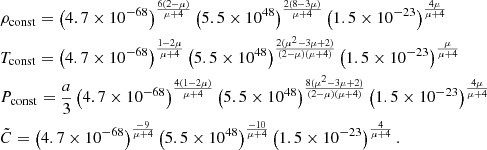 (A.2)
(A.2)
The solutions for gas pressure dominated regions, that are independent on the choice of μ in the viscosity law, are:
![Mathematical equation: $$ \begin{aligned}&\rho =14.44\,\, k_0^{-3/5} \xi ^{3/10} [\alpha _0m]^{-7/10} [\dot{m}J(r)]^{2/5} r^{-33/20} (1-\tilde{f})^{-3/10} \nonumber \\&T=8.01\times 10^{8}\,\, k_0^{-4/15} \xi ^{-1/5} [\alpha _0m]^{-1/5} [\dot{m}J(r)]^{2/5} r^{-9/10} (1-\tilde{f})^{1/5}\nonumber \\&h=1.72\times 10^{-2}\,\, k_0^{-7/15} \xi ^{-1/10} [\alpha _0m]^{-1/10} [\dot{m}J(r)]^{1/5} r^{21/20} (1-\tilde{f})^{1/10} \nonumber \\&P=1.91\times 10^{8}\,\, k_0^{-13/15} \xi ^{1/10} [\alpha _0m]^{-9/10} [\dot{m}J(r)]^{4/5} r^{-51/20} (1-\tilde{f})^{-1/10} \nonumber \\&\frac{4\alpha _0^2-k_1^4f^4}{k_1^4f^4}=5.41\times 10^{2}\, k_0^{-1/5} \xi ^{-9/10} [\alpha _0m]^{1/10} [\dot{m}J(r)]^{4/5} r^{-21/20} (1-\tilde{f})^{9/10}. \end{aligned} $$](/articles/aa/full_html/2019/08/aa35874-19/aa35874-19-eq58.gif) (A.3)
(A.3)
The value of ξ can be obtained by studying the continuity of all the above quantities at the boundary between the radiation pressure- to the gas pressure-dominated regions. It corresponds to  .
.
In Fig. A.1 we report examples of radial profiles for ρ, Ptot, κ, h/r, Tmid and Teff. Similar examples for f and L2 keV are shown in Fig. 1. Once fmax is fixed, the dominant variance among the models is given by the choice of the viscosity law (μ), while α0 plays a minor role. This is shown in Fig. A.2, where profiles for f and L2 keV show little difference in varying α0 from 0.02 to 0.2.
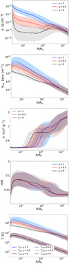 |
Fig. A.1. Same as Fig. 1, with radial profiles for the mid-plane ρ (top left), Ptot (gas plus radiation, top central), κ (top right), h/r (bottom left) and T (both mid-plane and surface, bottom right). |
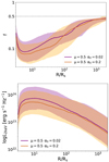 |
Fig. A.2. Same as in Figs. 1 and A.1. Here, we highlight the (minor) influence on varying α0 from 0.02 (purple) to 0.2 (orange) in f- and L2 keV-profiles. |
Appendix B: The reference AGN sample
For the source-by-source modeling of XMM-XXL we used the 379 sources obtained following the methodology outlined in Sect. 4.2. In Fig. B.1 we show the distribution of L2 keV (top panel) and L3000 Å (bottom panel) in the luminosity-redshift plane of the 379 sources (red and blue respectively), with respect to the parent sample of BLAGN from L16 (black). The LX − LUV slope of this reference sample is 0.54 ± 0.02, from Eq. (12). This is incompatibly flatter than the values quoted in the recent literature, namely 0.64 ± 0.02 (Lusso & Risaliti 2016) or 0.63 ± 0.02 (LR17). The cleaning criteria applied in Sect. 4.1 were aimed to exclude low-quality data and to be consistent with the model, while in the above-mentioned literature the possible biases of flux-limited samples were treated carefully in order to reliably use quasars for cosmology (Risaliti & Lusso 2019).
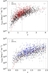 |
Fig. B.1. Distribution of L2 keV (top panel) and L3000 Å (bottom panel) in the luminosity-redshift plane of the 379 sources of our XMM-XXL sample (red and blue respectively), with respect to the parent sample of BLAGN from L16 (black). The dashed red lines broadly represent the sensitivity of the survey at the related frequency (see the text for a description). |
We investigated whether this inconsistency in the slope would be bridged restricting the analysis to the brightest objects at all redshifts with a very crude and conservative selection. From the sensitivity curve of the XXL-N survey in the 0.5 − 10 keV band at half of the survey area (L16, their Fig. 3) we obtained the flux limit in that energy band. Then, we interpolated the flux limit at 2 keV using the mean photon index of the sample, obtaining the sensitivity curve shown in red in the top panel of Fig. B.1. In Menzel et al. (2016) a cut at r < 22.5 mag was applied. We converted this magnitude limit in a luminosity sensitivity only within 0.80 ≲ z ≲ 1.27, for which 3000 Å was actually detected in the r band. For different redshifts, we first computed a redshift dependent color correction for the other bands (u, g, i and z) performing a linear regression on the difference with the r-band magnitude. This provided a magnitude limit for L3000 Å at all redshifts, consistently with the band in which that wavelength was actually detected, from which we obtained the related sensitivity line in the bottom panel of Fig. B.1. We then divided XMM-XXL in six redshift bins, making sure to have at least 30 counts per bin. For each bin, we excluded all the sources below the limits given by the sensitivity curves on both axis, evaluated at the maximum z of the bin to be conservative (Fig. B.2). The resulting cleanest subsample reaches accordance with the recent literature of the LX − LUV, with a slope of 0.59 ± 0.03.
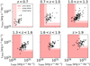 |
Fig. B.2. LX − LUV relation in the redshift bins reported in the sub-titles. The sensitivity surfaces at the minimum, median and maximum redshift of the bin are represented in red with a full area, a dashed line and a shaded area respectively. These surfaces are obtained from the sensitivity lines in Fig. B.1 at the above-mentioned redshifts. The sources above the shaded sensitivity area in each z-bin give the cleanest XMM-XXL sample. |
All Tables
All Figures
|
Fig. 1. Radial profiles for the fraction f of power dissipated in the corona (top panel) and L2 keV (bottom panel), obtained with fixed α0 = 0.02 and fmax = 0.5. Colors are coded according to the choice of the viscosity law: stress proportional to Ptot (Pgas + Prad, μ = 0, black), to Pgas (μ = 1, blue), or the geometric mean of the two (μ = 0.5, red). The continuous solid, or solid-dashed, lines represent the median profiles, with the related shaded areas showing the 16th and 84th percentiles, the scatter due to the range of sources (i.e. m and ṁ) modeled. L2 keV is proportional to the product of f and Q+ (the accretion power per unit area). As Q+ has very similar profiles across all models, those systems for which f is smaller produce weaker coronae in the central part. Top panel: a solid line for the median f-profile represents (thermally) stable regions of the median test source, whereas a dashed line highlights the instability regions. The vertical dot-dashed lines show instead where the median transition radius, from Prad- to Pgas-dominated regions, lies. Refer to Sect. 2.1 for details. |
| In the text | |
|
Fig. 2. Schematic illustration of our model and how it relates to the observed LX − LUV (see Sect. 3 for an interpretative guide). |
| In the text | |
|
Fig. 3. Mock LX − LUV with fixed fmax = 0.5 and different μ color coded, as in Fig. 1. The connected solid points show the trend of a single typical mass (log m = 8.7) with ṁ = 0.03, 0.07, 0.17, 0.42, 1 (increasing from left to right in LUV). The dashed lines indicate a slope of one. The distributions of transparent points show the mock LX − LUV for a range of |
| In the text | |
|
Fig. 4. LX − LUV relation of the 379 bright BLAGN of XMM-XXL. Monochromatic luminosity values are here scaled by 25 dex, to ease the comparison with recent works. The solid black line is the median regression line obtained with emcee, with the corresponding 16th and 84th percentiles represented with the shaded gray area. The dashed black lines show the intrinsic scatter around the median relation. |
| In the text | |
|
Fig. 5. The central panel of each image shows an example of the LX − LUV relation for both XMM-XXL (black stars) and the model (blue dots), in which the choice of μ, α0 and fmax is shown in the titles. The black and red solid lines are randomly drawn from the posterior distributions of normalization and slope for XMM-XXL and the model, respectively, with the median regression line thickened. The bottom panels show the residuals given by the difference of observed and mock log L2 keV and the right panels show the related distributions. The errors on the model are show in the bottom right corner of the central panels. |
| In the text | |
|
Fig. 6. r2 score, representing the goodness of match between XMM-XXL and mocks (see text), as a function of fmax. Models with μ = 0, 0.5, 1 are color coded in black, red and blue, respectively. The additional dependency on α0 is represented with varying line-types as shown in the legend, when present (it is absent for μ = 0). A good match is represented with a score greater than zero. The points include the uncertainties in the score values. The shaded areas represent the results obtained applying the same methodology on a different sample (RM-QSO, Liu et al., in prep.), fixing α0 = 0.02 and using the same colors. |
| In the text | |
|
Fig. 7. Top panel: the 2 keV-emission rpeak (r90) as a function of μ is represented in black (gray). The green shaded area qualitatively shows the inner radii, where the bulk of X-ray emission is supposed to come from according to X-ray reverberation and micro-lensing. For increasing μ, the X-ray emission profile peaks at larger radii. Middle panel: for increasing μ the models obtain a slope of the LX − LUV closer to the observed one. The dark-green area represents the reference slope of the cleanest XXM-XXL (Appendix B), while the light-green refers to the slope quoted in LR17. Bottom panel: intrinsic scatter of the mock LX − LUV relations as a function of μ. The green area represents a tentative upper limit of the true scatter (Lusso & Risaliti 2016; Chiaraluce et al. 2018), that is only due to the physical properties of AGN. For simplicity, all panels show only the results obtained with a single fmax, corresponding to the highest r2-score (e.g., Fig. 6), and fixed α0 = 0.02. |
| In the text | |
|
Fig. 8. 1-, 2- and 3-sigma contours of the emcee regressions in the slope-normalization ( |
| In the text | |
|
Fig. 9. Same as Fig. 8, with the addition of empty contours for μ = 0.4, 0.5 and 0.6 (color coded in the legend) obtained with maximally spinning black holes (i.e. with ϵ0 = 0.3 and r0 = 1.24rg). The dashed lines connect them to the non-spinning analogous realizations. Dark-red density spots represent the location of the center of different contours of the standard μ = 0.5 case, in which the only difference is the adoption of η (downward scattering component) varying among 0.4, 0.5 and 0.6, going from higher to lower |
| In the text | |
|
Fig. 10. LX − LUV relation for the high-spin model with μ = 0.5, α0 = 0.02 and fmax = 0.9 (empty red points, corresponding to the empty red contour in Fig. 9), with the red line showing best fit slope from emcee. The connected filled points (dark red) show the single-mass trend (log m = 8.7) for varying accretion rate (0.03, 0.07, 0.17, 0.42, 1). For a comparison, the black contour shows where the data lie in the plane, with the related best-fit slope (black line). |
| In the text | |
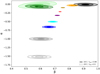 |
Fig. 11. Same as Fig. 8 with the addition of a reproduction of LR17’s toy-model as gray contours. |
| In the text | |
|
Fig. A.1. Same as Fig. 1, with radial profiles for the mid-plane ρ (top left), Ptot (gas plus radiation, top central), κ (top right), h/r (bottom left) and T (both mid-plane and surface, bottom right). |
| In the text | |
|
Fig. A.2. Same as in Figs. 1 and A.1. Here, we highlight the (minor) influence on varying α0 from 0.02 (purple) to 0.2 (orange) in f- and L2 keV-profiles. |
| In the text | |
|
Fig. B.1. Distribution of L2 keV (top panel) and L3000 Å (bottom panel) in the luminosity-redshift plane of the 379 sources of our XMM-XXL sample (red and blue respectively), with respect to the parent sample of BLAGN from L16 (black). The dashed red lines broadly represent the sensitivity of the survey at the related frequency (see the text for a description). |
| In the text | |
|
Fig. B.2. LX − LUV relation in the redshift bins reported in the sub-titles. The sensitivity surfaces at the minimum, median and maximum redshift of the bin are represented in red with a full area, a dashed line and a shaded area respectively. These surfaces are obtained from the sensitivity lines in Fig. B.1 at the above-mentioned redshifts. The sources above the shaded sensitivity area in each z-bin give the cleanest XMM-XXL sample. |
| In the text | |
Current usage metrics show cumulative count of Article Views (full-text article views including HTML views, PDF and ePub downloads, according to the available data) and Abstracts Views on Vision4Press platform.
Data correspond to usage on the plateform after 2015. The current usage metrics is available 48-96 hours after online publication and is updated daily on week days.
Initial download of the metrics may take a while.