| Issue |
A&A
Volume 663, July 2022
|
|
|---|---|---|
| Article Number | L4 | |
| Number of page(s) | 5 | |
| Section | Letters to the Editor | |
| DOI | https://doi.org/10.1051/0004-6361/202244105 | |
| Published online | 08 July 2022 | |
Letter to the Editor
Constraining X-ray emission of a magnetically arrested disk by radio-loud AGNs with an extreme-ultraviolet deficit
1
Key Laboratory for Research in Galaxies and Cosmology, Shanghai Astronomical Observatory, Chinese Academy of Sciences, 80 Nandan Road, Shanghai 200030, PR China
e-mail: lisl@shao.ac.cn; gumf@shao.ac.cn
2
University of Chinese Academy of Sciences, 19A Yuquan Road, 100049 Beijing, PR China
3
School of Physics and Electronic Information, Shangrao Normal University, 401 Zhimin Road, Shangrao 334001, PR China
e-mail: zhoumh8@163.com
Received:
24
May
2022
Accepted:
28
June
2022
Aims. Active galactic nuclei (AGNs) with an extreme-ultraviolet (EUV) deficit are suggested to be powered by a magnetically arrested disk (MAD) surrounding the black hole, where the slope of EUV spectra (αEUV) is found to possess a clearly positive relationship with the jet efficiency. In this work, we investigate the properties of X-ray emission in AGNs with an EUV deficit for the first time.
Methods. We constructed a sample of 15 objects with an EUV deficit to analyze their X-ray emission. The X-ray luminosity in 13 objects was recently processed by us, while the other two sources were gathered from archival data.
Results. It is found that the average X-ray flux of AGNs with an EUV deficit are 4.5 times larger than that of radio-quiet AGNs (RQAGNs), while the slope of the relationship between the optical-UV luminosity (LUV) and the X-ray luminosity (LX) is found to be similar with that of RQAGNs. For comparison, the average X-ray flux of radio-loud AGNs (RLAGNs) without an EUV deficit is about 2–3 times larger than that of RQAGNs. A strong positive correlation between αEUV and radio loudness (RUV) is also reported. However, there is no strong relationship between LX and the radio luminosity (LR).
Conclusions. Both the excess of X-ray emission of RLAGNs with an EUV deficit and the strong αEUV − RUV relationship can be qualitatively explained with the MAD scenario, which can help one to constrain the theoretical model of MAD.
Key words: accretion, accretion disks / black hole physics / magnetohydrodynamics (MHD) / galaxies: active / X-rays: galaxies
© S.-L. Li et al. 2022
 Open Access article, published by EDP Sciences, under the terms of the Creative Commons Attribution License (https://creativecommons.org/licenses/by/4.0), which permits unrestricted use, distribution, and reproduction in any medium, provided the original work is properly cited.
This article is published in open access under the Subscribe-to-Open model. Subscribe to A&A to support open access publication.
1. Introduction
About 10% of active galactic nuclei (AGNs) are observed to be accompanied by relativistic jets, which have been popular for several decades (see Blandford et al. 2019 for a review). There are mainly two jet-formation mechanisms in theory, that is to say the so-called Blandford–Znajek (BZ) mechanism (Blandford & Znajek 1977) and the Blandford–Payne (BP) mechanism (Blandford & Payne 1982). While BZ and BP mechanisms extract energy from a rotating black hole and accretion disk, respectively, both of them require the presence of large-scale magnetic fields. Large-scale magnetic fields are believed to play a key role in the formation of winds and jets (Blandford & Znajek 1977; Blandford & Payne 1982; Lubow et al. 1994; Spruit & Uzdensky 2005; Tchekhovskoy et al. 2011; McKinney et al. 2012; Bu et al. 2013; Blandford et al. 2019, etc.), though their origin is still debatable. One promising way of generating the large-scale magnetic fields is that the field line at an outer boundary can be effectively dragged inward and amplified with the accretion of gas. Usually the radial velocity in an accretion disk becomes faster with increasing disk scaled-height (Shakura & Sunyaev 1973). Therefore, the field line can be easily amplified in a geometrically thick accretion disk due to its shorter advection timescale than diffusive timescale (e.g., Lubow et al. 1994; Cao 2011), but it is very difficult for a standard thin disk with very slow radial velocity. However, this problem may be resolved when taking the magnetically driven winds into account, which can improve the radial velocity of gas by transferring a lot of angular momentum from the accretion disk (Cao & Spruit 2013; Li & Begelman 2014).
When more and more magnetic flux is accumulated in the inner region of a disk, the magnetic pressure is comparable or even higher than the gas pressure and thus the symmetry of the accretion disk is destroyed, leading to the generation of a magnetically arrested disk (MAD, e.g., Narayan et al. 2003). The magneto-rotational instability (MRI) is suppressed inside a MAD, but the gas can still be accreted slowly through a magnetic Rayleigh–Taylor (RT) instability (e.g., Marshall et al. 2018). The presence of a MAD has been validated by several general relativistic magnetohydrodynamic (GRMHD) simulations (e.g., Tchekhovskoy et al. 2011; McKinney et al. 2012; Morales Teixeira et al. 2018; White et al. 2019). In observations, the extreme-ultraviolet (EUV) emission in some radio-loud AGNs (RLAGNs) is obviously deficit compared with their radio-quiet counterparts (Telfer et al. 2002). This phenomenon had been suggested as evidence for the presence of a MAD (Punsly 2014, 2015, hereinafter P14 and P15). It is found that the spectral index in the EUV band (αEUV, fν ∼ ν−αEUV) has a positive correlation with the jet efficiency (ηjet = Qjet/Lbol, where Qjet and Lbol are the jet power and bolometric luminosity, respectively), which can be well fitted under the MAD scenario (P14 and P15). The size of MAD (Rm) given in this scenario is ∼5.5 gravitational radius (Rg = GM/C2) for a modestly rotating black hole. The EUV deficit is caused by the process in which a fraction of gravitational energy released between Rg and Rm may be transferred to a jet as Poynting flux by the islands of magnetic flux in a MAD (see P14 for details).
While previous studies mainly focused on the optical-UV properties of a MAD in RLAGNs, for the first time we try to investigate their X-ray properties in this work. The origin of X-ray emission in RLAGNs is still under debate, which may come from a corona, jet, or both. In observations, there is a big difference between the X-ray properties of radio-quiet AGNs (RQAGNs) and RLAGNs. Firstly, the average X-ray flux in RLAGNs is found to be 2–3 times higher than that in RQAGNs (e.g., Zamorani et al. 1981; Wilkes & Elvis 1987; Li & Gu 2021). Secondly, Laor et al. (1997) reported that RLAGNs have harder 2–10 kev X-ray spectra than RQAGNs by compiling a sample of 23 quasars observed with ROSAT, which was subsequently confirmed by Shang et al. (2011) with a larger sample. Comparing the X-ray spectrum of 3CRR quasars and that of radio-quiet quasars, Zhou & Gu (2020) also gave a similar result. In addition, the X-ray reflection features of RLAGNs are weaker than those of RQAGNs (Wozniak et al. 1998). All of these results seem to indicate that the contribution of a jet to X-ray spectra cannot be neglected. However, several recent works suggested a totally different result. First, the slope of LUV − LX is found to be consistent for RLAGNs and RQAGNs (Zhu et al. 2020, 2021; Li & Gu 2021). Second, Gupta et al. (2018, 2020) discovered that the distributions of X-ray photon spectral indices between RLAGNs and their radio-quiet counterpart are very similar (see Zhu et al. 2021 either). This opposite conclusion may be due to the effect of sample selection. The sample of Gupta et al. (2018, 2020) was X-ray selected (and optically selected for the sample of Zhu et al. 2021), which may lead to the radio jet power being very feeble compared to the bolometric luminosity in most of the RLAGNs. These weakly jetted RLAGNs can therefore have different X-ray photon indices compared to the strong jetted RLAGNs, such as the 3CRR quasars of Zhou & Gu (2020). P15 also indicated that the weakly jetted RLAGNs have similar αEUV as RQAGNs. However, interestingly, Markoff et al. (2005) demonstrated that both the corona model and the jet model can fit the X-ray data of some Galactic X-ray binaries well and that the jet base may be subsumed to corona in some ways. The 3CRR quasars are low frequency radio selected and have a strong jet on a large scale. However, it is still unclear whether all the objects with a strong jet harbor a MAD, or just containing MAD when jet is firstly launching millions of years ago. We focus on the RLAGNs with an EUV deficit in this work, which should possess a MAD in the inner disk region as suggested by P15. The presence of a MAD surrounding the black hole may bring a remarkable difference to the X-ray emissions since the structure of disk-corona greatly changes in the case of MAD (e.g., Tchekhovskoy et al. 2011; McKinney et al. 2012; White et al. 2019). In theory, it has been suggested that X-ray emission increases when an advection-dominated accretion flow (ADAF) becomes a MAD in its inner region (Xie & Zdziarski 2019). Nevertheless, how MAD affects the disk-corona corresponding to the X-ray emission of quasars is still an open issue. This work can constrain a future theoretical model for MAD in RLAGNs.
2. Sample
Based on the observations with Hubble Space Telescope (HST), Telfer et al. (2002) constructed a sample of 184 quasars to investigate their typical optical-UV spectral properties. The optical-UV continuum of RQAGNs and RLAGNs is found to be similar when the wavelength is longer than 1050 Å (Zheng et al. 1997; Telfer et al. 2002). However, when the wavelength shortens, αEUV of RLAGNs is found to be larger than that of RQAGNs, where αEUV of RQAGNs and RLAGNs were 1.57 ± 0.17 and 1.96 ± 0.12, respectively (Telfer et al. 2002). Combining this with the jet power, P15 tried to investigate the origin of the EUV deficit in RLAGNs and the distribution of magnetic flux tubes in the innermost disk region. All the objects in our sample were compiled from P15. In order to ensure the deficit of EUV emission, we adopted the objects with only αEUV ≥ 1.75. Fifteen out of 18 objects with αEUV ≥ 1.75 in P15 were found to be observed in X-ray (see Table 1). Among the 15 sources, except for 1022+194 taken from Brinkmann et al. (1997) and 0024+224 derived from NED1, the X-ray flux of the other 13 sources were found by us.
Sample.
Our X-ray data process of Chandra and XMM-Newton are described in Zhou & Gu (2020, 2021), and here we provide only an overview. All Chandra data were processed with Chandra Interactive Analysis of Observations software (CIAO) v4.12 and Chandra Calibration Database (CALDB) version 4.9.2.1 with CIAO threads2. We reprocessed Chandra archived data with the chandra_repro script, checked background flares, filtered energy between 0.3 and 7.0 keV, and inspected the piledup effect with the same method as in Zhou & Gu (2020). The source spectrum was finally extracted from source and background regions at a source-centered circle with a radius of 2.5″ and a 20–30″ annulus, respectively.
The original XMM-Newton X-ray data were reprocessed with the XMM-Newton Scientific Analysis Software (SAS) package. For better X-ray quality, we preferred to use a pn dataset which was processed with epproc in SAS-18.0.0 and was filtered in the energy range of 0.2 − 15.0 keV. We filtered out the time interval of large flares and checked the pileup effect. The source and background X-ray spectrum were then extracted from the source-centered radius of 32″ and the source-free region of 40″ around the object. Both Chandra and XMM-Newton X-ray spectra were fitted with an absorbed power-law model with fixed Galactic absorption (phabs * zphabs * powerlaw). Based on the fitting results of power-law parameters, we estimated the X-ray flux at 2 keV in Table 1.
We processed Swift X-ray spectra with the online XRT and UVOT data analysis tool3. With a series of input settings, a source name, a redshift, “All” observations, and some default settings, the online analysis tool presents the time-averaged X-ray spectrum for all observations and the corresponding power-law fitting results. Thus the flux at 2 keV can be calculated.
All the data in Cols. (1)–(3) were directly taken from P15. The spectral luminosity at 2500 Å (LUV) in Col. (4) were derived from LEUV at 1100 Å with a spectral index αo = −0.5 (fν = ναo, e.g., Shang et al. 2011), where LEUV at 1100 Å can be achieved from P15. Columns (5) and (6) are the hydrogen column density and photon index adopted to fit the X-ray data, respectively. The Δ log LX in Col. (8) represent the excess of X-ray luminosity observed and the X-ray flux calculated with the LUV − LX relationship given by Lusso et al. (2010) (see Sect. 3 for details). The radio core luminosity at 5 GHz (Col. (10)) were compiled from NED1. For sources without direct observations at 5 GHz, the luminosity was derived from the neighboring frequencies with a radio spectral index index of αR = −0.5 (fν ∼ ναR; e.g., Shang et al. 2011).
3. Results
By constructing a type-1 AGN sample of over 500 sources from the XMM-COSMOS survey, Lusso et al. (2010) investigated the optical-to-X-ray properties of AGNs and reported a tight positive relationship between X-ray luminosity and optical-UV luminosity in RQAGNs, that is to say log LX = 0.76 log LUV + 3.508. This relationship can be qualitatively fitted with the classical disk-corona model, where the X-ray flux comes from the inverse Compton scattering of a hot corona to the seed photon from an optically thick and geometrically thin accretion disk (Lusso & Risaliti 2017; Qiao & Liu 2018). A similar relationship has also been achieved in RLAGNs recently (Zhu et al. 2020; Li & Gu 2021). However, the X-ray flux in RLAGNs is found to be 2–3 times larger than that in RQAGNs (Zamorani et al. 1981; Wilkes & Elvis 1987; Gupta et al. 2018; Li & Gu 2021), though their slope is quite similar.
In Fig. 1, we investigate the correlation between LX at 2 kev and LUV at 2500 Å for the RLAGNs with a EUV deficit, where the blue line represents our best-fitting result and the green line is the best-fitting result for RQAGNs given by Lusso et al. (2010). The red line shows the LUV − LX relationship for RLAGNs without an EUV deficit, where the X-ray luminosity is two times (0.3 dex) higher than the green line (Zamorani et al. 1981; Wilkes & Elvis 1987; Gupta et al. 2018; Li & Gu 2021). We find that the X-ray emission in RLAGNs with an EUV deficit is, on average, 4.5 and 2.2 times higher than that in RQAGNs and RLAGNs without an EUV deficit, respectively. The relationship between LX and LUV can be given as follows:

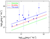 |
Fig. 1. Relationship between the X-ray luminosity LX and optical-UV luminosity LUV in RLAGNs with an EUV deficit, where the blue line represents our best-fitting result. The green line is the best-fitting result for RQAGNs given by Lusso et al. (2010). The red line corresponds to the relationship for RLAGNs without an EUV deficit. |
where the confidence level based on a Pearson test is about 99.0%.
We note that αEUV is found to be positively correlated with the jet efficiency ηjet, which can be understood with the MAD scenario in P15. The presence of a MAD indicates a stronger magnetic field strength in the region surrounding the black hole, which can improve both αEUV and the jet power. We further investigate the relationship between αEUV and the radio loudness RUV in this work, where RUV of all objects are found to be larger than 100 (typically higher than the 3CRR objects on average, see, e.g., Li & Gu 2021). A strong positive correlation is shown in Fig. 2, which reads as follows:

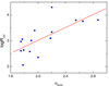 |
Fig. 2. Relationship between RUV and αEUV, where the red line represents the best-fitting result. |
where the confidence level based on a Pearson test is about 99.7%.
4. Discussion
The formation of a MAD affects both the inner region of a thin accretion disk and the corona above a disk, resulting in a deficit of EUV emissions. However, how a MAD will change the dynamics of a corona is unclear. Usually, a corona is believed to be compact and small, on the order of tens of gravitational radii or less (rg = GM/C2; e.g., Uttley et al. 2014), while the structure and composition of corona is still under debate (Ricci et al. 2018). A corona has been suggested to be similar with ADAF by some works (e.g., Liu et al. 2015; Qiao & Liu 2018). A MAD can greatly increase the radiative efficiency of ADAF, possibly due to the higher optical depth (see Xie & Zdziarski 2019 for details), which is qualitatively consistent with our results (see Fig. 1). Except for the X-ray excess, the LX − LUV slope between RLAGNs with an EUV deficit and RQAGNs is found to be well coincident (e.g., Lusso et al. 2010). Our results suggest that the X-ray emission in RLAGNs with an EUV deficit may originate from a MAD and can be applied to constrain the theoretical model for a MAD in the future.
The other possibility for the X-ray excess in RLAGNs with an EUV deficit is that the relativistic jet can also contribute to and even dominate the X-ray emission. If so, both the radio emission and X-ray emission should come from a jet, where the synchrotron radiation of an electron corresponding to the former provides the seed photon required by the latter to process the inverse-Compton scattering. Therefore, the radio luminosity LR should be strongly correlated with the X-ray luminosity LX (e.g., Heinz & Sunyaev 2003; Merloni et al. 2003). We further explore the LR − LX relationship in Fig. 3 to validate this assumption. However, no strong correlation is found between them, which indicates that the X-ray emission in RLAGNs with an EUV deficit may be dominated by an accretion disk. Furthermore, Li & Gu (2021) found a strong but steeper LR − LX relationship, that is log(LR/LEdd) = (2.0 ± 0.2)log(LX/LEdd)+0.3 ± 0.6, in RLAGNs by compiling a sample from the 3CRR catalog, which can also be qualitatively explained by the disk-corona model (see their paper for details). For comparison, a much shallower relationship of LR ∼ LX is reported in low-luminosity AGNs (Corbel et al. 2003; Merloni et al. 2003; Xie & Yuan 2016; Li & Gu 2018). Therefore, in summary, the X-ray emission in RLAGNs with an EUV deficit can reflect the effect of a MAD on a corona.
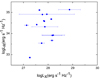 |
Fig. 3. Relationship between the radio spectral luminosity LR and the X-ray spectral luminosity LX. |
Except for the excess of the X-ray flux, we also report a strong relationship between αEUV and RUV (Fig. 2). We notice that a somewhat similar relationship of αEUV and ηjet (=Qjet/Lbol) was given in P15. However, the jet power Qjet in P15 was estimated with the radio emission at 151 MHz dominated by the lobe of a jet, which, however, represents the emission from jets a very long time ago, thus it is different from the present bolometric luminosity. We adopted the core emission at 5 GHz to calculate the radio loudness RUV in this work. Both the core radio emission and UV radiation are from current activity; therefore, the radio loudness RUV is a more reasonable indicator of jet efficiency when studying the properties of a MAD. In physics, increasing the magnetic field strength produces stronger radio luminosity LR in a jet (Blandford & Znajek 1977). Meanwhile, the stronger MAD due to an increasing magnetic field results in a higher EUV deficit (larger αEUV, see P15). Therefore, the positive αEUV − RUV relationship in Fig. 2 can be qualitatively understood under the scenario of a MAD.
5. Conclusions
In this Letter, we compile a sample to investigate the X-ray properties in RLAGNs with an EUV deficit which are suggested to be powered by a MAD. The X-ray flux in RLAGNs with an EUV deficit is found to be about 4.5 times larger than that in RQAGNs (Fig. 1). However, the slope of the LX − LUV relationship is found to be well consistent with that in RQAGNs (Lusso et al. 2010). In addition, the traditionally strong LR − LX relationship is absent in our sample. However, a strong positive relationship between the radio loudness RUV and αEUV is discovered (see Fig. 2). All of these results can help one to explore the theory for a MAD.
Acknowledgments
We thank the reviewer for his/her very helpful comments. SLL thanks Dr. Fuguo Xie and Erlin Qiao for valuable discussion on MAD. This work is supported by the NSFC (grants 11773056, 11873073), Shanghai Pilot Program for Basic Research – Chinese Academy of Science, Shanghai Branch (JCYJ-SHFY-2021-013), and the science research grants from the China Manned Space Project with NO. CMSCSST-2021-A06. MZ is supported by the Science and Technology Project funded by the Education Department of Jiangxi Province in China (Grant No. GJJ211733), and the Doctoral Scientific Research Foundation of Shangrao Normal University (Grant No. K6000449). This work has made extensive use of the NASA/IPAC Extragalactic Database (NED), which is operated by the Jet Propulsion Laboratory, California Institute of Technology, under contract with the National Aeronautics and Space Administration (NASA).
References
- Blandford, R. D., & Payne, D. G. 1982, MNRAS, 199, 883 [CrossRef] [Google Scholar]
- Blandford, R. D., & Znajek, R. L. 1977, MNRAS, 179, 433 [NASA ADS] [CrossRef] [Google Scholar]
- Blandford, R., Meier, D., & Readhead, A. 2019, ARA&A, 57, 467 [NASA ADS] [CrossRef] [Google Scholar]
- Brinkmann, W., Yuan, W., & Siebert, J. 1997, A&A, 319, 413 [NASA ADS] [Google Scholar]
- Bu, D.-F., Yuan, F., Wu, M., & Cuadra, J. 2013, MNRAS, 434, 1692 [NASA ADS] [CrossRef] [Google Scholar]
- Cao, X. 2011, ApJ, 737, 94 [NASA ADS] [CrossRef] [Google Scholar]
- Cao, X., & Spruit, H. C. 2013, ApJ, 765, 149 [NASA ADS] [CrossRef] [Google Scholar]
- Corbel, S., Nowak, M. A., Fender, R. P., Tzioumis, A. K., & Markoff, S. 2003, A&A, 400, 1007 [NASA ADS] [CrossRef] [EDP Sciences] [Google Scholar]
- Gupta, M., Sikora, M., Rusinek, K., & Madejski, G. M. 2018, MNRAS, 480, 2861 [NASA ADS] [CrossRef] [Google Scholar]
- Gupta, M., Sikora, M., & Rusinek, K. 2020, MNRAS, 492, 315 [NASA ADS] [CrossRef] [Google Scholar]
- Heinz, S., & Sunyaev, R. A. 2003, MNRAS, 343, L59 [Google Scholar]
- Laor, A., Fiore, F., Elvis, M., Wilkes, B. J., & McDowell, J. C. 1997, ApJ, 477, 93 [Google Scholar]
- Li, S.-L., & Begelman, M. C. 2014, ApJ, 786, 6 [NASA ADS] [CrossRef] [Google Scholar]
- Li, S.-L., & Gu, M. 2018, MNRAS, 481, L45 [NASA ADS] [CrossRef] [Google Scholar]
- Li, S.-L., & Gu, M. 2021, A&A, 654, A141 [NASA ADS] [CrossRef] [EDP Sciences] [Google Scholar]
- Liu, B. F., Taam, R. E., Qiao, E., & Yuan, W. 2015, ApJ, 806, 223 [NASA ADS] [CrossRef] [Google Scholar]
- Lubow, S. H., Papaloizou, J. C. B., & Pringle, J. E. 1994, MNRAS, 267, 235 [NASA ADS] [Google Scholar]
- Lusso, E., & Risaliti, G. 2017, A&A, 602, A79 [NASA ADS] [CrossRef] [EDP Sciences] [Google Scholar]
- Lusso, E., Comastri, A., Vignali, C., et al. 2010, A&A, 512, A34 [NASA ADS] [CrossRef] [EDP Sciences] [Google Scholar]
- Markoff, S., Nowak, M. A., & Wilms, J. 2005, ApJ, 635, 1203 [NASA ADS] [CrossRef] [Google Scholar]
- Marshall, M. D., Avara, M. J., & McKinney, J. C. 2018, MNRAS, 478, 1837 [NASA ADS] [CrossRef] [Google Scholar]
- McKinney, J. C., Tchekhovskoy, A., & Blandford, R. D. 2012, MNRAS, 423, 3083 [Google Scholar]
- Merloni, A., Heinz, S., & di Matteo, T. 2003, MNRAS, 345, 1057 [Google Scholar]
- Morales Teixeira, D., Avara, M. J., & McKinney, J. C. 2018, MNRAS, 480, 3547 [NASA ADS] [CrossRef] [Google Scholar]
- Narayan, R., Igumenshchev, I. V., & Abramowicz, M. A. 2003, PASJ, 55, L69 [NASA ADS] [Google Scholar]
- Punsly, B. 2014, ApJ, 797, L33 [NASA ADS] [CrossRef] [Google Scholar]
- Punsly, B. 2015, ApJ, 806, 47 [NASA ADS] [CrossRef] [Google Scholar]
- Qiao, E., & Liu, B. F. 2018, MNRAS, 477, 210 [NASA ADS] [CrossRef] [Google Scholar]
- Ricci, C., Ho, L. C., Fabian, A. C., et al. 2018, MNRAS, 480, 1819 [NASA ADS] [CrossRef] [Google Scholar]
- Shakura, N. I., & Sunyaev, R. A. 1973, A&A, 24, 337 [NASA ADS] [Google Scholar]
- Shang, Z., Brotherton, M. S., Wills, B. J., et al. 2011, ApJS, 196, 2 [Google Scholar]
- Spruit, H. C., & Uzdensky, D. A. 2005, ApJ, 629, 960 [NASA ADS] [CrossRef] [Google Scholar]
- Tchekhovskoy, A., Narayan, R., & McKinney, J. C. 2011, MNRAS, 418, L79 [NASA ADS] [CrossRef] [Google Scholar]
- Telfer, R. C., Zheng, W., Kriss, G. A., & Davidsen, A. F. 2002, ApJ, 565, 773 [NASA ADS] [CrossRef] [Google Scholar]
- Uttley, P., Cackett, E. M., Fabian, A. C., Kara, E., & Wilkins, D. R. 2014, A&ARv, 22, 72 [NASA ADS] [CrossRef] [Google Scholar]
- White, C. J., Stone, J. M., & Quataert, E. 2019, ApJ, 874, 168 [Google Scholar]
- Wilkes, B. J., & Elvis, M. 1987, ApJ, 323, 243 [Google Scholar]
- Wozniak, P. R., Zdziarski, A. A., Smith, D., Madejski, G. M., & Johnson, W. N. 1998, MNRAS, 299, 449 [NASA ADS] [CrossRef] [Google Scholar]
- Xie, F.-G., & Yuan, F. 2016, MNRAS, 456, 4377 [Google Scholar]
- Xie, F.-G., & Zdziarski, A. A. 2019, ApJ, 887, 167 [NASA ADS] [CrossRef] [Google Scholar]
- Zamorani, G., Henry, J. P., Maccacaro, T., et al. 1981, ApJ, 245, 357 [NASA ADS] [CrossRef] [Google Scholar]
- Zheng, W., Kriss, G. A., Telfer, R. C., Grimes, J. P., & Davidsen, A. F. 1997, ApJ, 475, 469 [NASA ADS] [CrossRef] [Google Scholar]
- Zhou, M., & Gu, M. 2020, ApJ, 893, 39 [NASA ADS] [CrossRef] [Google Scholar]
- Zhou, M.-H., & Gu, M.-F. 2021, Res. Astron. Astrophys., 21, 004 [CrossRef] [Google Scholar]
- Zhu, S. F., Brandt, W. N., Luo, B., et al. 2020, MNRAS, 496, 245 [Google Scholar]
- Zhu, S. F., Timlin, J. D., & Brandt, W. N. 2021, MNRAS, 505, 1954 [NASA ADS] [CrossRef] [Google Scholar]
All Tables
All Figures
|
Fig. 1. Relationship between the X-ray luminosity LX and optical-UV luminosity LUV in RLAGNs with an EUV deficit, where the blue line represents our best-fitting result. The green line is the best-fitting result for RQAGNs given by Lusso et al. (2010). The red line corresponds to the relationship for RLAGNs without an EUV deficit. |
| In the text | |
|
Fig. 2. Relationship between RUV and αEUV, where the red line represents the best-fitting result. |
| In the text | |
|
Fig. 3. Relationship between the radio spectral luminosity LR and the X-ray spectral luminosity LX. |
| In the text | |
Current usage metrics show cumulative count of Article Views (full-text article views including HTML views, PDF and ePub downloads, according to the available data) and Abstracts Views on Vision4Press platform.
Data correspond to usage on the plateform after 2015. The current usage metrics is available 48-96 hours after online publication and is updated daily on week days.
Initial download of the metrics may take a while.