| Issue |
A&A
Volume 622, February 2019
|
|
|---|---|---|
| Article Number | A135 | |
| Number of page(s) | 45 | |
| Section | Interstellar and circumstellar matter | |
| DOI | https://doi.org/10.1051/0004-6361/201629777 | |
| Published online | 08 February 2019 | |
ATLASGAL-selected massive clumps in the inner Galaxy
VII. Characterisation of mid-J CO emission★
1
Max-Planck-Institut für Radioastronomie,
Auf dem Hügel 69,
53121
Bonn,
Germany
e-mail: This email address is being protected from spambots. You need JavaScript enabled to view it.
2
Universidade de São Paulo, Instituto de Astronomia, Geofísica e Ciências Atmosféricas, Departamento de Astronomia, Rua do Matão 1226, Cidade Universitária São Paulo-SP,
05508-090,
Brazil
3
INAF – Osservatorio Astronomico di Cagliari,
Via della Scienza 5,
09047
Selargius (CA),
Italy
4
INAF – Istituto di Radioastronomia & Italian ALMA Regional Centre,
Via P. Gobetti 101,
40129
Bologna,
Italy
5
Centre for Astrophysics and Planetary Science, The University of Kent,
Canterbury,
Kent CT2 7NH,
UK
Received:
22
September
2016
Accepted:
17
December
2018
Abstract
Context. High-mass stars are formed within massive molecular clumps, where a large number of stars form close together. The evolution of the clumps with different masses and luminosities is mainly regulated by their high-mass stellar content and the formation of such objects is still not well understood.
Aims. In this work, we characterise the mid-J CO emission in a statistical sample of 99 clumps (TOP100) selected from the ATLASGAL survey that are representative of the Galactic proto-cluster population.
Methods. High-spatial resolution APEX-CHAMP+ maps of the CO (6–5) and CO (7–6) transitions were obtained and combined with additional single-pointing APEX-FLASH+ spectra of the CO (4–3) line. The data were convolved to a common angular resolution of 13.′′4. We analysed the line profiles by fitting the spectra with up to three Gaussian components, classified as narrow or broad, and computed CO line luminosities for each transition. Additionally, we defined a distance-limited sample of 72 sources within 5 kpc to check the robustness of our analysis against beam dilution effects. We have studied the correlations of the line luminosities and profiles for the three CO transitions with the clump properties and investigate if and how they change as a function of the evolution.
Results. All sources were detected above 3-σ in all three CO transitions and most of the sources exhibit broad CO emission likely associated with molecular outflows. We find that the extension of the mid-J CO emission is correlated with the size of the dust emission traced by the Herschel-PACS 70 μm maps. The CO line luminosity (LCO) is correlated with the luminosity and mass of the clumps. However, it does not correlate with the luminosity-to-mass ratio.
Conclusions. The dependency of the CO luminosity with the properties of the clumps is steeper for higher-J transitions. Our data seem to exclude that this trend is biased by self-absorption features in the CO emission, but rather suggest that different J transitions arise from different regions of the inner envelope. Moreover, high-mass clumps show similar trends in CO luminosity as lower mass clumps, but are systematically offset towards larger values, suggesting that higher column density and (or) temperature (of unresolved) CO emitters are found inside high-mass clumps.
Key words: astrochemistry / stars: formation / stars: protostars / ISM: molecules / ISM: kinematics and dynamics / line: profiles
Tables A.1–A.7 are only available at the CDS via anonymous ftp to cdsarc.u-strasbg.fr (130.79.128.5) or via http://cdsarc.u-strasbg.fr/viz-bin/qcat?J/A+A/622/A135
© ESO 2019
1 Introduction
High-mass stars are responsible for the dynamical and chemical evolution of the interstellar medium and of their host galaxies by injecting heavier elements and energy in their surrounding environment by means of their strong UV emission and winds. Despite their importance, the processes that lead to the formation of high-mass stars are still not well understood (Zinnecker & Yorke 2007).
Observations at high-angular resolution have confirmed a high degree of multiplicity for high-mass stars, suggesting these objects are not formed in isolated systems (Grellmann et al. 2013). The same scenario is supported by three-dimensional simulations of high-mass star formation (Krumholz et al. 2009; Rosen et al. 2016). These objects are formed on a relatively short timescale (~105 yr), requiring large accretion rates (~10−4 M⊙ yr−1, Hosokawa & Omukai 2009). Such conditions can only be achieved in the densest clumps in molecular clouds, with sizes of ≲ 1 pc and masses of order 100–1000 M⊙ (Bergin & Tafalla 2007). These clumps are associated with large visual extinctions, thus observations at long wavelengths are required to study their properties and the star formation process.
After molecular hydrogen (H2), which is difficult to observe directly in dense cold gas, carbon monoxide (CO) is the most abundant molecular species. Thus, rotational transitions of CO are commonly used to investigate the physics and kinematics of star-forming regions (SFRs). Traditionally, observations of CO transitions with low angular momentum quantum number J from J = 1–0 to 4–3 (here defined as low-J transitions) have been used for this purpose (e.g., see Schulz et al. 1995; Zhang et al. 2001; Beuther et al. 2002). These lines have upper level energies, Eu, lower than 55 K and are easily excited at relatively low temperatures and moderate densities. Therefore, low-J CO lines are not selective tracers of the densest regions of SFRs, but are contaminated by emission from the ambient molecular cloud. On the other hand, higher-J CO transitions are less contaminated by ambient gas emission and likely probe the warm gas directly associated with embedded young stellar objects (YSOs). In this paper, we make use of the J = 6–5 and 7–6 lines of CO, with Eu ~ 116 K and 155 K, respectively, and in the following we refer to them simply as mid-J CO transitions. Over the past decade the Atacama Pathfinder Experiment telescope (APEX1, Güsten et al. 2006) has enabled routine observations of mid-J CO lines, while Herschel and SOFIA have opened the possibility of spectroscopically resolved observations of even higher-J transitions (J = 10–9 and higher, e.g. Gómez-Ruiz et al. 2012; San José-García et al. 2013, hereafter, SJG13; Leurini et al. 2015; Mottram et al. 2017). van Kempen et al. (2009a, hereafter, vK09) and van Kempen et al. (2009b) have shown the importance of mid-J CO transitions in tracing warm gas in the envelopes and outflows of low-mass protostars. More recently, SJG13 used the High Frequency Instrument for the Far Infrared (HIFI, de Graauw et al. 2010) on board of Herschel to study a sample of low- and high-mass star-forming regions in high-J transitions of several CO isotopologues (e.g. CO, 13CO and C18O J = 10−9), finding that the link between entrained outflowing gas and envelope motions is independent of the source mass.
In this paper, we present CO (6–5) and CO (7–6) maps towards a sample of 99 high-mass clumps selected from the APEX Telescope Large Area Survey of the Galaxy (ATLASGAL), which has provided an unbiased coverage of the plane of the inner Milky Way in the continuum emission at 870 μm (Schuller et al. 2009). Complementary single-pointing observations of the CO (4–3) line are also included in the analysis in order to characterise the CO emission towards the clumps. Section 2 describes the sample and Sect. 3 presents theobservations and data reduction. In Sect. 4 we present the distribution and extent of the mid-J CO lines and their line profiles, compute the CO line luminosities and the excitation temperature of the gas, and compare them with the clump properties. In Sect. 5 we discuss our results in the context of previous works. Finally, the conclusions are summarised in Sect. 6.
2 Sample
ATLASGAL detected the vast majority of all current and future high-mass star forming clumps (Mclump > 1000 M⊙) in the innerGalaxy. Recently, Urquhart et al. (2018) completed the distance assignment for ~97% of the ATLASGAL sources and analysed their masses, luminosities and temperatures based on thermal dust emission, and discussed how these properties evolve. Despite the statistical relevance of the ATLASGAL sample, detailed spectroscopic observationsare not feasible on the whole sample. Therefore, we defined the ATLASGAL Top 100 (hereafter, TOP100, Giannetti et al. 2014; König et al. 2017), a flux-limited sample of clumps selected from this survey with additional infrared (IR) selection criteria to ensure it encompasses a full range of luminosities and evolutionary stages (from 70 μm-weak quiescent clumps to H II regions). The 99 sources analysed in this paper are a sub-sample of the original TOP100 (König et al. 2017) and are classified as follows:
clumps which either do not display any point-like emission in the Hi-GAL Survey (Molinari et al. 2010) 70 μm images and (or) only show weak, diffuse emission at this wavelength (hereafter, 70w, 14 sources);
mid-IR weak sources that are either not associated with any point-like counterparts or the associated compact emission is weaker than 2.6 Jy in the MIPSGAL survey (Carey et al. 2009) 24 μm images (hereafter IRw, 31 sources);
mid-IR bright sources in an active phase of the high-mass star formation process, with strong compact emission seen in 8 μm and 24 μm images, but still not associated with radio continuum emission (hereafter IRb, 33 sources);
sources in a later phase of the high-mass star formation process that are still deeply embedded in their envelope, but are bright in the mid-IR and associated with radio continuum emission (H II regions, 21 sources).
König et al. (2017) analysed the physical properties of the TOP100 sample in terms of distance, mass and luminosity. They found that at least 85% of the sources have the ability to form high-mass stars and that most of them are likely gravitationally unstable and would collapse without the presence of a significant magnetic field. These authors showed that the TOP100 represents a statistically significant sample of high-mass star-forming clumps covering a range of evolutionary phases, from the coldest and quiescent 70 μm-weak to the most evolved clumps hosting H II regions, with no bias in terms of distance, luminosity and mass among the different classes. The masses and bolometric luminosities of the clumps range from ~20 to 5.2 × 10⁵ M⊙ and from ~60 to 3.6 × 10⁶ L⊙, respectively. The distance of the clumps ranges between 0.86 and 12.6 kpc, and 72 of the 99 clumps have distances below 5 kpc. This implies that observationsof the TOP100 at the same angular resolution sample quite different linear scales. In Table A.1, we list the main properties of the observed sources. We adopted the Compact Source Catalogue (CSC) names from Contreras et al. (2013) for the TOP100 sample although the centre of the maps may not exactly coincide with those positions (the average offset is ~5.′′4, with valuesranging between ~0.′′5 and 25.′′ 8, see Table A.1).
In this paper, we investigate the properties of mid-J CO lines for a sub-sample of the original TOP100 as part of our effort to observationally establish a solid evolutionary sequence for high-mass star formation. In addition to the dust continuum analysis of König et al. (2017), we further characterised the TOP100 in terms of the content of the shocked gas in outflows traced by SiO emission (Csengeri et al. 2016) and the ionised gas content (Kim et al. 2017), the CO depletion (Giannetti et al. 2014), and the progressive heating of gas due to feedback of the central objects (Giannetti et al. 2017; Tang et al. 2018). These studies confirm an evolution of the targeted properties with the original selection criteria and strengthen our initial idea that the TOP100 sample constitutes a valuable inventory of high-mass clumps in different evolutionary stages.
3 Observations and data reduction
3.1 CHAMP+ observations
Observations of the TOP100 sample were performed with the APEX 12-m telescope on the following dates of 2014 May 17–20, July 10, 15–19, September 9–11 and 20. The CHAMP+ (Kasemann et al. 2006; Güsten et al. 2008) multi-beam heterodyne receiver was used to map the sources simultaneously in the CO (6–5) and CO (7–6) transitions. Information about the instrument setup configuration is given in Table 1.
The CHAMP+ array has 2 × 7 pixels that operate simultaneously in the radio frequency tuning ranges 620–720 GHz in the low frequency array (LFA) and the other half in the range 780–950 GHz in the high frequency array (HFA), respectively. The half-power beam widths (θmb) are 9.′′ 0 (at 691 GHz) and 7.′′ 7 (807 GHz), and the beam-spacing is ~2.15 θmb for both sub-arrays. The observations were performed in continuous on-the-fly (OTF) mode and maps of 80′′ × 80′′ size, centredon the coordinates given in Table A.1, were obtained for each source. The area outside of the central 60′′ × 60′′ region of each map is covered by only one pixel of the instrument, resulting in a larger rms near the edges of the map. The sky subtraction was performed by observing a blank sky field, offset from the central positions of the sources by 600′′ in right ascension. The average precipitable water vapour (PWV) of the observations varied from 0.28 to 0.68 mm per day, having a median value of 0.50 mm. The average system temperatures (Tsys) ranged from 1050 to 1550 K and 3500 to 6500 K, at 691 and 807 GHz, respectively. Pointing and focus were checked on planets at the beginning of each observing session. The pointing was also checked every hour on Saturn and Mars, and on hot cores (G10.47+0.03 B1, G34.26, G327.3−0.6, and NGC6334I) during the observations.
Each spectrum was rest-frequency corrected and baseline subtracted using the “Continuumand Line Analysis Single Dish Software” (CLASS), which is part of the GILDAS software2. The data were binned to a final spectral resolution of 2.0 km s−1 in order to improve the signal-to-noise ratio of the spectra. The baseline subtraction was performed using a first-order fit to the line-free channels outside a window of ±100 km s−1 wide, centred on the systemic velocity, Vlsr, of each source. We used a broader window for sources exhibiting wings broader than ~80 km s−1 (AGAL034.2572+00.1535, AGAL301.136−00.226, AGAL327.393+00.199, AGAL337.406− 00.402, AGAL351. 244+00.669 and AGAL351.774−00.537, see Table A.6). Antenna temperatures ( ) were converted to main-beam temperatures (Tmb) using beam efficiencies of 0.41 at 691 GHz and 0.34 at 809 GHz3. Forward efficiencies are 0.95 in all observations. The gridding routine XY_MAP in CLASS was used to construct the final datacubes. This routine convolves the gridded data with a Gaussian of one third of the beam telescope size, yielding a final angular resolution slightly coarser (9.′′ 6 for CO (6–5) and 8.′′ 2 for CO (7–6)) than the original beam size (9.′′ 0 and 7.′′ 7, respectively). The final spectra at the central position of the maps have an average rms noise of 0.20 and 0.87 K for CO (6–5) and CO (7–6) data, respectively.
Figure 1 presents the ratio between the daily integrated flux and the corresponding average flux for the CO (6–5) transition of each hot core used as calibrator as a function of the observing day. The deviation of the majority of the points with respect to their average value is consistent within a ±20% limit; thus, this value was adopted as the uncertainty on the integrated flux for both mid-J CO transitions. On September 10, the observations of G327.3−0.6 showed the largest deviation from the average flux of the source (points at y ~ 0.7 and y ~ 0.5 in Fig. 1). For this reason, we associate an uncertainty of 30% on the integrated flux of the sources AGAL320.881−00.397, AGAL326.661+00.519 and AGAL327.119+00.509, and of 50% for sources AGAL329.066−00.307 and AGAL342.484+00.182, observed immediately after these two scans on G327.3−0.6.
Summary of the observations.
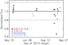 |
Fig. 1 Ratio between the daily integrated flux and the average flux of the CO (6–5) transition for the calibration sources observed during the campaign. A solid horizontal line is placed at 1.0 and the dashed lines indicate a deviation of 20% from unity. |
3.2 FLASH+ observations
The FLASH+ (Klein et al. 2014) heterodyne receiver on the APEX telescope was used to observe the central positions of the CHAMP+ maps in CO (4–3) on 2011 June 15 and 24, August 11 and 12. Table 1 summarises the observational setup. The observations were performed in position switching mode with an offset position of 600′′ in right ascension for sky-subtraction. Pointing and focus were checked on planets at the beginning of each observing session. The pointing was also regularly checked during the observations on Saturn and on hot cores (G10.62, G34.26, G327.3−0.6, NGC6334I and SGRB2(N)). The average PWV varied from 1.10 to 1.55 mm per day with a median value of 1.29 mm. The system temperatures of the observations ranged from 650 to 2150 K.
The single-pointing observations were processed using GILDAS/CLASS software. The data were binned to a final spectral resolution of 2.0 km s−1 and a fitted line was subtracted to stablish a straight baseline. The antenna temperatures were converted to Tmb by assuming beam and forward efficiencies of 0.60 and 0.95, respectively. The resulting CO (4–3) spectra have an average rms noise of 0.36 K. The uncertainty on the integrated flux of FLASH+ data was estimated to be ~20% based on the continuum flux of the sources observed during the pointing scans.
3.3 Spatial convolution of the mid-J CO data
The CO (6–5) and CO (7–6) data were convolved to a common angular resolution of 13.′′ 4, matching the beam size of the single-pointing CO (4–3) observations. The resulting spectra are shown in Appendix B.
The median rms of the convolved spectra are 0.35 K, 0.17 K and 0.87 K for the CO (4–3), CO (6–5) and CO (7–6) transitions, respectively. These values differ from those reported in Table 1 for the CHAMP+ data where the rms at the original resolution of the dataset is given. Since our sources are not homogeneously distributed in distance (see Sect. 2), spectra convolved to the same angular resolution of 13.′′ 4 sample linear scales between 0.06 and 0.84 pc. In order to study the effect of any bias introduced by sampling different linear scales within the clumps, the CO (6–5) and CO (7–6) data were also convolved to the same linear scale, ℓlin, of ~0.24 pc, which corresponds to an angular size θ (in radians) of:
 (1)
(1)
that depends on the distance of the source. The choice of ℓlin is driven by the nearest source, AGAL353.066+00.452, for which the part of the map with a relatively uniform rms (see Sect. 3.1) corresponds to a linear scale of ~0.24 pc. Since we are limited by the beam size of the CO (6–5) observations (~10′′), the same projected length can be obtained only for sources located at distances up to ~5.0 kpc. This limit defines a sub-sample of 72 clumps (ten 70w, 20 IRw, 26 IRb and 16 H II regions).
The rest of the paper focuses on the properties of the full TOP100 sample based on the spectra convolved to 13.′′4. The properties of the distance-limited sub-sample differ from those of the 13.′′ 4 data only for the line profile (see Sect. 4.2). A detailed comparison between the CO line luminosity and the properties of the clumps for the distance-limited sample is presented in Appendix C.1.
3.4 Self-absorption and multiple velocity components
The CO spectra of several clumps show a double-peak profile close to the ambient velocity (e.g. AGAL12.804−00.199, AGAL14.632−00.577, and AGAL333.134−00.431, see Fig. B.1). These complex profiles could arise from different velocity components in the beam or could be due to self-absorption given the likely high opacity of CO transitions close to the systemic velocity. To distinguish between these two scenarios, the 13.′′ 4 CO spectra obtained in Sect. 3.3 were compared to the C17 O (3–2) data from Giannetti et al. (2014) observed with a similar angular resolution (19′′). In the absence of C17O observations (AGAL305.192−00.006, AGAL305.209+00.206 and AGAL353.066+00.452), the C18O (2–1) profiles were used. Since the isotopologue line emission is usually optically thin (cf. Giannetti et al. 2014), it provides an accurate determination of the systemic velocity of the sources and, therefore, can be used to distinguish between the presence of multiple components or self-absorption in the optically thick 12CO lines. Thus, when C17O or C18O show a single peak corresponding in velocity to a dip in CO, we consider the CO spectra to be affected by self-absorption. Otherwise, if also the isotopologue data show a double-peak profile, the emission is likely due to two different velocity components within the beam. From the comparison with the CO isotopologues, we find 83 clumps with self-absorption features in the CO (4–3) line, 79 in the CO (6–5), 70 in the CO (7–6) transition. These numbers indicate that higher-J CO transitions tend to be less affected by self-absorption features when compared to the lower-J CO lines. Finally, only 15 objects do not display self-absorption features in any transitions. The CO spectra affected by self-absorption features are flagged with an asterisk symbol in Table A.6.
To assess the impact of self-absorption on the analysis presented in Sect. 4.3, in particular on the properties derived from the integrated flux of the CO lines, we compared the observed integrated intensity of each CO transition with the corresponding values obtained from the Gaussian fit presented in Sect. 3.5. This comparison indicated that self-absorption changes the offsets and the scatter of the data but not the slopes of the relations between the CO emission and the clump properties. Then, we investigated the ratio between the observed and the Gaussian integrated intensity values as a function of the evolutionary classes of the TOP100 sample. We found that 95% of the sources exhibit ratios between 0.7 and 1.0 for all three lines. We also note a marginal decrease on the ratios from the earliest 70w class (~1.0) to H II regions (~0.8), indicating that self-absorption does not significantly affect the results presented in the following sections. We further investigated the effects of self-absorption by studying the sub-sample of ~15 sources not affected by self-absorption (that is, the sources that are not flagged with an asterisk symbol in Table A.6) and verified that the results presented in the following sections for the full sample are consistent with those of this sub-sample, although spanning a much broader range of clump masses and luminosities. More details on the analysis of the robustness of the relations reported in Sect. 4.3 are provided in Appendices C.1 and C.2. Five sources (see Appendix C.3) show a second spectral feature in the 12CO transitions and in the isotopologue data of Giannetti et al. (2014) shifted in velocity from the rest velocity of the source. We compared the spatial distribution of the integrated intensity CO (6–5) emission with the corresponding ATLASGAL 870 μm images (see Fig. C.5) for these five clumps. We found that in all sources the morphology of the integrated emission of one of the two peaks (labelled as P2 in Tables A.2–A.4) has a different spatial distribution than the dust emission at 870 μm and, thus, is likely not associated with the TOP100 clumps. These components are excluded from any further analysis in this paper.
3.5 Gaussian decomposition of the CO profiles
The convolved CO spectra were fitted using multiple Gaussian components. The fits were performed interactively using the MINIMIZE task in CLASS/GILDAS. A maximum number of three Gaussian components per spectrum was adopted. Each spectrum was initially fitted with one Gaussian component: if the residuals had substructures larger than 3-σ, a second or even a third component was added. In case of self-absorption (see Sect. 3.4), the affected channels were masked before performing the fit. Any residual as narrow as the final velocity resolution of the data (2.0 km s−1) was ignored.In particular for CO (4–3), absorption features shifted in velocity from the main line are detected in several sources. These features are likely due to emission in the reference position, and were also masked before fitting the data. Examples of the line profile decomposition are given in Fig. 2.
Each component was classified as narrow (N) or broad (B), adopting the scheme from San José-García et al. (2013). According to their definition, the narrow component has a full-width at half maximum (FWHM) narrower than 7.5 km s−1, otherwise it is classified as a broad component. Results of the Gaussian fit are presented in Tables A.2–A.4. In several cases, two broad components are needed to fit the spectrum. For the CO (6–5) data, 29 of the profiles required 3 components and, thus, two or three components have received the same classification. In these cases, they were named as, for example, B1, B2; ordered by their width. The P2 features mark secondary velocity components not associated with TOP100 clumps (see Sect. 3.4).
As a consequence of high opacity and self-absorption, the Gaussian decomposition of the line profile can be somewhat dubious. In some cases, and in particular for the CO (4–3) transition, the fit is unreliable (e.g. AGAL305.192−00.006 and AGAL333.134−00.431 in Fig. B.1). The sources associated with unreliable Gaussian decomposed CO profiles (32, 8 and 4 for CO (4–3), CO (6–5) and CO (7–6), respectively) are not shown in Tables A.2–A.4 and their data are not included in the analysis presented in Sect. 4, as well as in that of the integrated properties of their line profiles (e.g. their integrated intensities and corresponding line luminosities, see Sect. 4.3).
The general overview of the fits are given in Table 2 and the statistics of FWHM of the narrow and broad Gaussian components are listed in Table 3. The spectrum of each source with its corresponding decomposition into Gaussian components is presented in Fig. B.1.
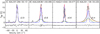 |
Fig. 2 Gaussian decomposition for the CO (6–5) line using up to 3 components. Panel A: single Gaussian fit; panel B: two-components fit; panel C: two-components fit (channels affected by self absorption are masked); panel D: three-components fit (channels affected by self absorption are masked). The spectra, fits and residuals were multiplied by the factor shown in each panel. The Gaussian fits are shown in blue, green and yellow, ordered by their line width; the sum of all components is shown in red. The grey lines indicate the baseline and the dashed horizontal lines placed in the residuals correspond to the 3-σ level. Self-absorption features larger than 5-σ were masked out from the residuals. |
Results of the Gaussian fit of the CO spectra convolved to a common angular resolution of 13.′′ 4.
Statistics of the FWHM of the Gaussian components fitted on the CO line profiles convolved to a common angular resolution of 13.′′4.
4 Observational results
The whole sample was detected above a 3-σ threshold in the single-pointing CO (4–3) data (source AGAL301.136−00.226 was not observed with FLASH+) and in the 13.′′ 4 CO (6–5) and CO (7–6) spectra, with three 70w sources (AGAL030.893 +00.139, AGAL351.571+00.762 and AGAL353.417−00.079) only marginally detected above the 3-σ limit in CO (7–6).
In the rest of this section we characterise the CO emission towards the TOP100 sample through the maps of CO (6–5) (Sect. 4.1) and the analysis of the CO line profiles for the spectra convolved to 13.′′ 4 (Sect. 4.2). In Sect. 4.3, we compute the CO line luminosities and compare them with the clump properties. Finally, in Sect. 4.4 we compute the excitation temperature of the gas.
4.1 Extent of the CO emission
In Fig. 3 we present examples of the integrated intensity maps of the CO (6–5) emission as a function of the evolutionary class of the TOP100 clumps. The CO (6–5) maps of the full TOP100 sample are presented in Appendix B (see Fig. B.1).
We estimated the linear size of the CO emission, Δs, defined as the average between the maximum and minimum elongation of the half-power peak intensity (50%) contour level of the CO (6–5) integrated intensity (see Table A.5). The uncertainty on Δs was estimated as the dispersion between the major and minor axis of the CO extent. The linear sizes of the CO emission ranges between 0.1 and 2.4 pc, with a median value of 0.5 pc. In order to investigate if Δs varies with evolution, we performed a non-parametric two-sided Kolmogorov–Smirnov (KS) test between pairs of classes (i.e. 70w vs. IRb; IRw vs. H II). The sub-samples were considered statistically different if their KS rank factor is close to 1 and associated with a low probability value, p (p ≤ 0.05 for a significance ≥ 2 σ). Our analysis indicates that there is no significant change in the extension of CO with evolution (KS ≤ 0.37, p ≥ 0.05 for all comparisons). The CO extent was further compared with the bolometric luminosity, Lbol, and the mass of the clumps, Mclump, reported by König et al. (2017). The results are presented in Fig. 4. Δs shows a large scatter as a function of Lbol while it increases with Mclump (ρ = 0.72, p < 0.001 for the correlation with Mclump ρ = 0.42, p < 0.001 for Lbol, where the ρ is the Spearman rank correlation factor and p its associated probability). This confirms that the extent of the CO emission is likely dependent of the amount of gas within the clumps, but not on their bolometric luminosity.
We derived the extent of the 70 μm emission (Δs70 μm) towards the 70 μm-bright clumps by cross-matching the position of the TOP100 clumps with the sources from Molinari et al. (2016). Then, Δs70 μm was obtained by computing the average between the maximum and minimum FWHM reported on their work and the corresponding error was obtained as the standard deviation of the FWHM values. The values are also reported in Table A.5. Figure 5 compares the extent of the CO (6–5) emission with that of the 70 μm emission towards the 70 μm bright clumps. The extent of the emission of CO (6–5) and of the 70 μm continuum emission are correlated (Fig. 5, ρ = 0.67, p < 0.001), and in the majority of cases, the points are located above the equality line, suggesting that the gas probed by the CO (6–5) transition tends to be more extended than the dust emission probed by the PACS data towards the 70 μm-bright clumps.
 |
Fig. 3 Distribution of the CO (6–5) emission of four representative clumps of each evolutionary classes of the TOP100 clumps. The CO contours are presented on top of the Herschel-PACS maps at 70 μm. Each 70 μm map is scaled in according to the colour bar shown in the corresponding panel. The CO contours correspond to the emission integrated over the full-width at zero power (FWZP) of the CO (6–5) line, andthe contour levels are shown from 20% to 90% of the peak emission of each map, in steps of 10%. The position of the CSC source from Contreras et al. (2013) is shown as a × symbol. Thebeam size of the CO (6–5) observations is indicated in the left bottom region. |
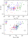 |
Fig. 4 Size ofthe CO (6–5) emission towards the TOP100 sample versus the bolometric luminosity (top panel) and the mass (bottom panel) of the sources. The median values for each class are shown as open diamonds and their error bars correspond to the absolute deviation of the data from their median value. The typical uncertainty is shown by the error bars on the bottom right of each plot. |
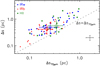 |
Fig. 5 Size of the CO (6–5) emission versus the size of the 70 μm emission from the Herschel-PACS images towards the 70 μm-bright clumps. The dashed line indicates y = x. The median values for the 70 μm-bright classes are shown as open diamonds and their error bars correspond to the absolute deviation of the data from their median value. The typical uncertainty, computed as the dispersion between the major and minor axis of the emission, is shown by the error bars on the bottom right of each plot. |
4.2 Line profiles
In the majority of the cases, the CO profiles are well fit with two Gaussian components, one for the envelope, one for high-velocity emission (see Table 2). A third component is required in some cases, in particular for the CO (6–5) data, which have the highest signal-to-noise ratio. We note that the majority of sources fitted with a single Gaussian component are in the earliest stages of evolution (70w and IRw clumps), suggesting that the CO emission is less complex in earlier stages of high-mass star formation. We also detect non-Gaussian high-velocity wings likely associated with outflows in most of the CO (6–5) profiles. A detailed discussion of the outflow content in the TOP100 sample and of their properties will be presented in a forthcoming paper (Navarete et al., in prep.).
To minimise biases due to different sensitivities in the analysis of single spectra, we computed the average CO spectrum of each evolutionary class and normalised it by its peak intensity. The spectra were shifted to 0 km s−1 using the correspondent Vlsr given in Table A.1. Then, the averaging was performed by scaling the intensity of each spectrum to the median distance of the sub-sample (d = 3.26 kpc for the distance-limited sample, d = 3.80 kpc for the full sample). The resulting spectra of the 13.′′4 dataset are shown in Fig. 6 while those of the distance-limited sub-sample are presented in Appendix C.1 (Fig. C.1). While the 13.′′ 4 data show no significant difference between the average profiles of IRw and IRb classes, in the distance-limited sub-sample the width (expressed through the full width at zero power, FWZP, to avoid any assumption on the profile) and the intensity of the CO lines progressively increase with the evolution of the sources (from 70w clumps towards H II regions) especially when the normalised profiles are considered. The difference between the two datasets is due to sources at large distances (d > 12 kpc; AGAL018.606−00.074, AGAL018.734−00.226 and AGAL342.484+00.182) for which the observations sample a much larger volume of gas. The increase of line width with evolution is confirmed by the analysis of the individual FWZP values of the three CO lines, presented in Table A.6 (see Table 4 for the statistics on the full TOP100 sample).
Despite the possible biases in the analysis of the line profiles (e.g. different sensitivities, different excitation conditions, complexity of the profiles), our data indicate that the CO emission is brighter in late evolutionary phases. The average spectra per class show also that the CO lines becomes broader towards more evolved phases likely due to the presence of outflows. Our study extends the work of Leurini et al. (2013) on one source of our sample, AGAL327.293−00.579. They mapped in CO (3–2), CO (6–5), CO (7–6) and in 13CO (6–5), 13CO (8–7) and 13CO (10–9) a larger area of the source than that presented here and found that, for all transitions, the spectra are dominated in intensity by the H II region rather than by younger sources (a hot core and an infrared dark cloud are also present in the area). They interpreted this result as an evidence that the bulk of the Galactic CO line emission comes from PDRs around massive stars, as suggested by Cubick et al. (2008) for FIR line emission. Based on this, we suggest that the increase in mid-J CO brightness in the later stages of the TOP100 is due to a major contribution of PDR to the line emission. We notice however that the increase of width and of intensity of the CO lines with evolution can also be due to an increase with time of multiplicity of sources in the beam.
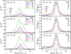 |
Fig. 6 Left panels: average CO (4–3), CO (6–5) and CO (7–6) spectra convolved to 13.′′ 4 beam of each evolutionary class scaled to the median distance of the whole sample (d = 3.80 kpc). Right panels: same plot, but the average CO spectra are normalised by their peak intensity. The baseline level is indicated by the solid grey line and the black dashed line is placed at 0 km s−1. The FWZP of the profiles are shown in the upper right side of the panels (in km s −1 units), together with the integrated intensities (Sint, in K kms−1 units) of theCO profiles shown in the left panels. |
Statistics on the CO line profiles, convolved to a common angular resolution of 13.′′ 4.
4.3 The CO line luminosities
The intensity of the CO profiles (Sint, in K km s−1) was computed by integrating the CO emission over the velocity channels within the corresponding FWZP range. Then, the line luminosity (LCO, in K km s−1 pc2) of each CO line was calculated using equation (2) from Wu et al. (2005), assuming a source of size equal to the beam size of the data (see Sect. 3.3). The derived LCO values are reported in Table A.6. The errors in the LCO values are estimated by error propagation on the integrated flux (see Sect. 3.1) and considering an uncertainty of 20% in the distance. The median values of LCO, Lbol, Mclump and L∕M, the luminosity-to-mass ratio, per evolutionary class are summarised in Table 5. We also performed the same analysis on the data convolved to a common linear scale of 0.24 pc (assuming the corresponding angular source size of 0.24 pc to derive the line luminosity) and no significant differences in the slope of the trends were found. Therefore, the distance-limited sample will not be discussed any further in this section.
In Fig. 7, we show the cumulative distribution function (CDF) of the line luminosities for the three CO transitions: LCO increases from 70w sources towards H II regions. Each evolutionary class was tested against the others by computing their two-sided KS coefficient (see Table 6). The most significant differences are found when comparing the earlier and later evolutionary classes (70w and IRb, 70w and H II, ρ ≥ 0.66 for the CO (6–5) line), while no strong differences are found among the other classes (KS ≤ 0.5 and p ≥ 0.003 for the CO (6–5) transition). These results indicate that, although we observe an increase on the CO line luminosity from 70w clumps towards H II regions, no clear separation is found in the intermediate classes (IRw and IRb, see also Table 5).
We also plot LCO against the bolometric luminosity of the clumps (Fig. 7), their mass and their luminosity-to-mass ratio (Figs. 8 and 9 for the CO (6–5) line). The L∕M ratio is believed to be a rough estimator of evolution in the star formation process for both low- (Saraceno et al. 1996) and high-mass regimes (e.g. Molinari et al. 2008), with small L∕M values corresponding to embedded regions where (proto-)stellar activity is just starting, and high L∕M values in sources with stronger radiative flux and that have accreted most of the mass (Molinari et al. 2016; Giannetti et al. 2017; Urquhart et al. 2018). In addition, the L∕M ratio also reflects the properties of the most massive young stellar object embedded in the clump (Faúndez et al. 2004; Urquhart et al. 2013a). The fits were performed using a Bayesian approach, by adjusting a model with three free parameters (the intercept, α, the slope, β, and the intrinsic scatter, ϵ). In order to obtain a statistically reliable solution, we computed a total of 100 000 iterations per fit. The parameters of the fits are summarised in Table 7. The correlation between LCO and the clump properties was checked by computing their Spearman rank correlation factor and its associated probability (ρ and p, respectively, see Table 8). Since LCO with Lbol and Mclump have the same dependence on the distance of the source, a partial Spearman correlation test was computed and the partial coefficient, ρp, was obtained (see Table 8).
In the right panel of Fig. 7, we show the CO line luminosity versus the bolometric luminosity of the TOP100 clumps. The plot indicates that LCO increases with Lbol over the entire Lbol range covered by the TOP100 clumps (~102–106 L⊙). The Spearman rank test confirms that both quantities are well correlated for all CO lines (ρ ≥ 0.7, with p < 0.001), even when excluding the mutual dependence on distance (ρp ≥ 0.81). The results of the fits indicate a systematic increase in the slope of LCO versus Lbol for higher-J transitions: 0.55 ± 0.05, 0.63 ± 0.03 and 0.68 ± 0.03 for the CO (4–3), CO (6–5) and CO (7–6), respectively. For the CO (6–5) and CO (7–6) lines, however, the slopes are consistent in within 2-σ. Concerning the dependence of the CO luminosity on Mclump (see Fig. 8), the partial correlation tests indicates that the distance of the clumps plays a more substantial role in the correlation found between LCO and Mclump (0.48 ≤ρp ≤ 0.57) than in the correlations found for LCO vs. Lbol. Finally, we do not find any strong correlation between the CO line luminosity and L∕M (ρ ≤ 0.5 for all transitions) although the median LCO values per class do increase with L∕M (Fig. 9). These findings are discussed in more detail in Sect. 5.
We further tested whether the steepness of the relations between LCO and the clump properties is not affected by self-absorption by selecting only those clumps which do not show clear signs of self-absorption (see Sect. 3.5). This defines a sub-sample of 15 sources in the CO (4–3) line, 18 in the CO (6–5) line and 26 objects in the CO (7–6) transition. These sources are highlighted in Figs. 7–9. Then, we repeated the fit of the relations between LCO and the clump properties using these sub-samples, finding no significant differences in the slopes of the relations presented in Table 7. The result of the fits for the sub-sample of sources with no signs of self-absorption in their 13.′′ 4 spectra are summarised in Table 9 and the correlations between LCO and the clump properties are listed in Table 10. The correlations are systematically weaker due to the smaller number of points than those obtained for the whole TOP100 sample (see Table 8). We found that the derived slopes for the relations between LCO and Lbol increases from 0.58 ± 0.09 to 0.71 ± 0.07, from the CO (4–3) to the CO (7–6) transition. Despite the larger errors in these relations, the slopes of the fits performed on these sources are not significantly different from those found for the whole TOP100 sample, confirming that at least the slopes of the relations found for the whole TOP100 sample are robust in terms of self-absorption effects. In addition, similar results were also found for the relations between LCO and the mass of the clumps, while no strong correlation between LCO and L∕M was found for this sub-sample.
Median values per class of the clump and CO profile properties.
Kolmogorov–Smirnov statistics of the CO line luminosity as a function of the evolutionary class of the clumps.
Parameters of the fits of LCO as a function of the clump properties.
Spearman rank correlation statistics for the CO line luminosity as a function of the clump properties towards the TOP100 sample.
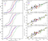 |
Fig. 7 Left panels: cumulative distribution function of the line luminosity of the CO (4–3) (upper panel), CO (6–5) (middle panel) and CO (7–6) emission (bottom panel) towards the TOP100 sample. The median values per class are shown as vertical dashed lines in their corresponding colours. Right panels: Line luminosity of the same CO J-transitions versus the bolometric luminosity of the TOP100 sources. The median values for each class are shown as open diamonds and their error bars correspond to the absolute deviation of the data from their median value. Data points highlighted in yellow indicate those sources from which no signs of self-absorption features where identified in the spectrum convolved to 13.′′ 4. The typical error bars are shown at the bottom right side of the plots. The black solid line is the best fit, the light grey shaded area indicates the 68% uncertainty, and the dashed lines show the intrinsic scatter (ϵ) of the relation. |
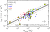 |
Fig. 8 Same as the right panel of Fig. 7, but displaying the line luminosity of the CO (6–5) emission as a function of the mass of the clumps. Data points highlighted in yellow indicate those sources from which no signs of self-absorption features where identified in the spectrum convolved to 13.′′ 4. |
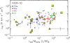 |
Fig. 9 Same as the right panel of Fig. 7, but displaying LCO of the CO (6–5) line as a function of the L∕M ratio of the TOP100 sources. Data points highlighted in yellow indicate those sources from which no signs of self-absorption features where identified in the spectrum convolved to 13.′′ 4. |
Parameters of the fits of LCO as a function of the clump properties for the TOP100 clumps that are not affected by self-absorption features.
Spearman rank correlation statistics for the CO line luminosity as a function of the clump properties for the TOP100 clumps that are not affected by self-absorption features.
4.4 The excitation temperature of the CO gas
The increase of LCO with the bolometric luminosity of the source (see Fig. 7) suggests that the intensity of the CO transitions may depend on an average warmer temperature of the gas in the clumps due to an increase of the radiation field from the central source (see for example van Kempen et al. 2009a). To confirm this scenario, we computed the excitation temperature of the gas, Tex, and compared it with the properties of the clumps.
Ideally, the intensity ratio of different CO transitions well separated in energy (e.g. CO (4–3) and CO (7–6)) allows a determination of the excitation temperature of the gas. However, most of the CO profiles in the TOP100 clumps are affected by self-absorption (see Sect. 3.4), causing a considerable underestimate of the flux especially in CO (4–3) and leading to unreliable ratios. Moreover, the CO (6–5) and CO (7–6) lines are too close in energy to allow a reliable estimate of the temperature. Alternatively, the excitation temperature can be estimated using the peak intensity of optically thick lines. From the equation of radiative transport, the observed main beam temperature (Tmb) can be written in terms of Tex as:
![Mathematical equation: \begin{equation*} T_{\rm{mb}} = \frac{h \nu}{k} \left[J_{\nu}(T_{\rm{ex}})-J_{\nu}(T_{\rm{bg}})\right] \left[ 1 - \exp\left(-\tau_{\nu} \right) \right]\vspace*{-5pt}\end{equation*}](/articles/aa/full_html/2019/02/aa29777-16/aa29777-16-eq3.png) (2)
(2)
where ![Mathematical equation: $J_{\nu}(T) = \left[\textrm{exp}(h \nu / k T) -1\right]^{-1}$](/articles/aa/full_html/2019/02/aa29777-16/aa29777-16-eq4.png) , Tbg is the background temperature and τν is the opacity of the source at the frequency ν. In the following, we include only the cosmic background as background radiation. Assuming optically thick emission (τν ≫ 1), Tex is given by:
, Tbg is the background temperature and τν is the opacity of the source at the frequency ν. In the following, we include only the cosmic background as background radiation. Assuming optically thick emission (τν ≫ 1), Tex is given by:
![Mathematical equation: \begin{equation*} T_{\rm{ex}} = \frac{h \nu / k}{\textrm{ln}\left[ 1 + \frac{h \nu / k}{T_{\rm{mb}} + (h \nu / k) J_{\nu}(T_{\rm{bg}})} \right]}.\end{equation*}](/articles/aa/full_html/2019/02/aa29777-16/aa29777-16-eq5.png) (3)
(3)
We computed Tex using the peak intensity of the CO (6–5) line from the Gaussian fit (Sect. 3.5) and also from its maximum observed value. Since CO (6–5) may be affected by self-absorption, the maximum observed intensity likely results in a lower limit of the excitation temperature. The values derived using both methods are reported in Table A.7. Tex derived from the peak intensity of the Gaussian fit ranges between 14 and 143 K, with a median value of 35 K. The analysis based on the observed intensity delivers similar results (Tex values range between 14 and 147 K, with a median value of 34 K).
The temperature of the gas increases with the evolutionary stage of the clumps and is well correlated with Lbol (ρ = 0.69, p < 0.001, see Fig. 10c). No significant correlation is found with Mclump (ρ = 0.09, p = 0.37). On the other hand, the excitation temperature is strongly correlated with L∕M (ρ = 0.72, p < 0.001), suggesting a progressive warm-up of the gas in more evolved clumps. We further compared the Tex values obtained from CO with temperature estimates based on other tracers (C17O (3–2), methyl acetylene, CH3CCH, ammonia, and the dust, Giannetti et al. 2014, 2017; König et al. 2017; Wienen et al. 2012). All temperatures are well correlated (ρ ≥ 0.44, p, < 0.001), however, the warm-up of the gas is more evident in the other molecular species than in CO (cf. Giannetti et al. 2017 and the KS tests reported in Table 11).
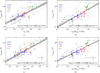 |
Fig. 10 Excitation temperature of the CO (6–5) line versus the bolometric luminosity of the TOP100 clumps (left panels) and the luminosity-to-mass ratio (right panels). The excitation temperature was derived using the peak of the Gaussian fit of the CO profiles. The median values for each class are shown as open diamonds and their error bars correspond to the median absolute deviation of the data from their median value. The black solid line is the best fit, the light grey shaded area indicates the 68% uncertainty, and the dashed lines show the intrinsic scatter (ϵ) of the relation. The best fit to the data is indicated by the filled black line. |
Kolmogorov–Smirnov statistics of the excitation temperature of the CO (6–5) line as a function of the evolutionary class of the clumps.
5 Discussion
5.1 Opacity effects
In Sect. 3.4 we found that self-absorption features are present in most of the CO spectra analysed in this work. To address this, we investigated the effects of self-absorption on our analysis and concluded that they are negligible since more than 80% of the CO integrated intensities are recovered in the majority of the sources (Sect. 3.5). We also verified that the steepness of the relations between LCO and the clump properties is not affected by self-absorption (Sect. 4.3).
In addition, the CO lines under examination are certainly optically thick, and their opacity is likely to decrease with J. Indeed, the comparison between LCO for differentCO transitions and the bolometric luminosity of the clumps (see Sect. 4.3) suggests a systematic increase in the slope of the relations as a function of J (see Table 7 for the derived power-law indices for LCO versus Lbol). Such a steepening of the slopeswith J is even more evident when including the relation found by San José-García et al. (2013) for CO (10–9) line luminosity in a complementary sample of the TOP100. For the CO (10–9) transition, they derived, log (LCO) = (−2.9 ± 0.2) + (0.84 ± 0.06) log(Lbol), which is steeper than the relations found towards lower-J transitions reported in this work. In Sect. 5.4 we further discuss SJG13 results by analysing their low- and high-mass YSO sub-samples. Our findings suggest that there is a significant offset between the sub-samples, leading to a much steeper relation between LCO and Lbol when considering their whole sample. However, the individual sub-samples follow similar power-law distributions, with power-law indices of (0.70 ± 0.08) and (0.69 ± 0.21) for the high- and low-mass YSOs, respectively.
In Fig. 11, we present the distribution of the power-law indices of the LCO versus Lbol relations, βJ, as a function of their corresponding upper-level J number, Jup. We include also the datapoint from the Jup = 10 line for the high-mass sources of SJG13 (see also discussion in Sect. 5.4). The best fit to the data, βJ = (0.44 ± 0.11) + (0.03 ± 0.02) Jup, confirms that the power-law index βJ gets steeper with J.
The fact that the opacity decreases with J could result in different behaviours of the line luminosities with Lbol for different transitions. This effect was recently discussed by Benz et al. (2016) who found that the value of the power-law exponents of the line luminosity of particular molecules and transitions depends mostly on the radius where the line gets optically thick. In the case of CO lines, the systematic increase on the steepness of the LCO versus Lbol relation with J (see Table 7) suggests that higher J lines trace more compact gas closer to the source and, thus, a smaller volume of gas is responsible for their emission. Therefore, observations of distinct J transitions of the CO molecule, from CO (4–3) to CO (7–6) (and even higher J transitions, considering the CO (10–9) data from SJG13), suggest thatthe line emission arises and gets optically thick at different radii from the central sources, in agreement with Benz et al. (2016).
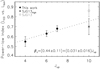 |
Fig. 11 Power-law indices of the LCO versus Lbol relations for different J transitions as a function of the upper-level J number. Theβ indices from Table 7 (filled black circles) are plotted together with data from SJG13 (open grey circle, excluded from the fit) and the exponent derived for their high-luminosity sub-sample (* symbol, see Fig. 12). The best fit is indicated by the dashed black line. |
5.2 Evolution of CO properties with time
In Sect. 4.3, we showed that LCO does not correlatewith the evolutionary indicator L∕M. This result is unexpected if we consider that in TOP100 the evolutionaryclasses are quite well separated in L∕M (with median values of 2.6, 9.0, 40 and 76 for 70w, IRw, IRb and H II regions, respectively, König et al. 2017).
Previous work on SiO in sources with similar values of L∕M as those of the TOP100 (e.g. Leurini et al. 2014; Csengeri et al. 2016) found that the line luminosity of low-excitation SiO transitions does not increase with L∕M, while the line luminosity of higher excitation SiO lines (i.e. Jup > 3) seems to increase with time. Those authors interpreted these findings in terms of a change of excitation conditions with time which is not reflected in low excitation transitions. This effect likely applies also to low- and mid-J CO lines with relatively low energies (≤155 K); higher-J CO transitions could be more sensitive to changes in excitation since they have upper level energies in excess of 300 K (e.g. CO (10–9) or higher J CO transitions). This hypothesis is strengthened by our finding that the excitation temperature of the gas increases with L∕M (see Fig. 10d). This scenario can be tested with observations of high-J CO transitions which are now made possible by the SOFIA telescope in the range Jup = 11–16. Also Herschel-PACS archive data could be used despite their coarse spectral resolution.
5.3 Do embedded HII regions still actively power molecular outflows?
In Sect. 4.2 we showed that H II regions have broad CO lines (see Fig. 6) likely associated with high-velocity outflowing gas. The H II sources in our sample are either compact or unresolved objects in the continuum emission at 5 GHz. Their envelopes still largely consist of molecular gas and have not yet been significantly dispersed by the energetic feedback of the YSOs. Our observations suggest that high-mass YSOs in this phase of evolution still power molecular outflows and are therefore accreting. This result is in agreement with the recent study of Urquhart et al. (2013b) and Cesaroni et al. (2015) who suggested that accretion might still be present during the early stages of evolution of H II regions based on the finding that the Lyman continuum luminosity of several H II regions appears in excess of that expected for a zero-age main-sequence star with the same bolometric luminosity. Such excess could be due to the so-called flashlight effect (e.g. Yorke & Bodenheimer 1999), where most of the photons escape along the axis of a bipolar outflow. Indeed Cesaroni et al. (2016) further investigated the origin of the Lyman excess looking for infall and outflow signatures in the same sources. They found evidence for both phenomena although with low-angular resolution data. Alternatively, the high-velocity emission seen in CO in the TOP100 in this work and in SiO in the ultra-compact H II regions of Cesaroni et al. (2016) could be associated with other younger unresolved sources in the clump and not directly associated with the most evolved object in the cluster. Clearly, high angular resolution observations (e.g. with ALMA) are needed to shed light on the origin of the high-velocity emission and confirm whether indeed the high-mass YSO ionising the surrounding gas is still actively accreting.
5.4 CO line luminosities from low- to high-luminosity sources
In this section, we further study the correlation between LCO and the bolometric luminosity of the clumps for different CO transitions to investigate the possible biases that can arise when comparing data with very different linear resolutions. This is important in particular when comparing galactic observations to the increasing number of extragalactic studies of mid- and high-J CO lines (e.g. Weiß et al. 2007; Decarli et al. 2016). We use results from SJG13 for the high energy CO (10–9) line (with a resolution of ~20′′) and from the CO (6–5) and CO (7–6) transitions observed with APEX by vK09. The sources presented by SJG13 cover a broad range of luminosities (from <1 L⊙ to ~105 L⊙) and are in different evolutionary phases. On the other hand, the sample studied by vK09 consists of eight low-mass YSOs with bolometric luminosities ≲30 L⊙.
To investigate the dependence of the line luminosity in different CO transitions on Lbol from low- to high-mass star-forming clumps, we first divided the sources from SJG13 into low- (Lbol < 50 L⊙) and high-luminosity (Lbol > 50 L⊙) objects. In this way and assuming the limit Lbol = 50 L⊙ adopted by SJG13 as a separation between low- and high-mass YSOs, we defined a sub-sample of low-mass sources (the targets of vK09 for CO (6–5) and CO (7–6), and those of SJG13 with Lbol < 50 L⊙ for CO J = 10−9) and one of intermediate- to high-mass clumps (the TOP100 for the mid-J CO lines and the sources from SJG13 with Lbol > 50 L⊙ for CO (10–9)).
In the upper panels of Fig. 12 we compare our data with those of vK09 for the CO (6–5) and CO (7–6) transitions. We could not include the sources of SJG13 in this analysis because observations in the CO (6–5) or CO (7–6) lines are not available. We calculated the CO line luminosity of their eight low-mass YSOs using the integrated intensities centred on the YSO on scales of ~0.01 pc (see their Table 3). In order to limit biases due to different beam sizes, we recomputed the CO luminosities from the central position of our map at the original resolution of the CHAMP+ data (see Table 1), probing linear scales ranging from ~0.04 to 0.6 pc. We performed three fits on the data: we first considered only the original sources of vK09 and the TOP100 separately, and then combined both samples. The derived power-law indices of the CO (6–5) data are 0.59 ± 0.25 and 0.59 ± 0.04 for the low- and high-luminosity sub-samples, respectively. Although the power-law indices derived for the two sub-samples are consistent within 1-σ, the fits are offset by roughly one order of magnitude (from −2.75 to −1.54 dex), indicating that LCO values are systematically larger towards high-luminosity sources. Indeed, the change on the offsets explains reasonably well the steeper power-law index found when combining both sub-samples (0.74 ± 0.03). Similar results are found for CO (7–6), although the difference between the offsets are slight smaller (~0.8 dex). The bottompanel of Fig. 12 presents the CO (10–9) luminosity for the SJG13 sample withthe best fit of their low- and high-luminosity sources separately. The derived power-law indices are 0.69 ± 0.21 and 0.70 ± 0.08 for the low- andhigh-luminosity sub-samples, respectively. The fits are offset by roughly 0.3 dex, which also explains the steeper slope of 0.84 ± 0.06 found by SJG13 when fittingthe two sub-samples simultaneously.
We interpret the shift in CO line luminosities between low- and high-luminosity sources as a consequenceof the varying linear resolution and sampled volume of gas of the data across the Lbol axis. In high-mass sources, mid-J CO lines trace extended gas (see the maps presented in Figs. B.1 for the TOP100) probably due to the effect of clustered star formation. Since the data presented in Fig. 12 are taken with comparable angular resolutions, the volume of gas sampled by the data is increasing with Lbol because sources with high luminosities are on average more distant. For the CO (10–9) data, the two sub-samples are likely differently affected by beam dilution. In close-by low-mass YSOs, the CO (10–9) line is dominated by emission from UV heated outflow cavities (van Kempen et al. 2010) and therefore is extended. In high-mass YSOs, the CO (10–9) line is probably emitted in the inner part of passively heated envelope (Karska et al. 2014) and therefore could suffer from beam dilution. This could explain the smaller offset in the CO (10–9) line luminosity between the low- and high-luminosity sub-samples.
SJG13 and San José-García et al. (2016) found a similar increase in the slope of the line luminosity of the CO (10−9) and of H2 O transitions versus Lbol when including extragalactic sources (see Fig. 14 of SJG13 and Fig. 9 of San José-García et al. 2016). These findings clearly outline the difficulties of comparing observations of such different scales and the problems to extend Galactic relations to extragalactic objects.
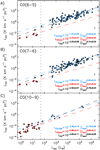 |
Fig. 12 CO line luminosity as a function of the bolometric luminosity for the CO (6–5) (upper panel), CO (7–6) (middle panel) and CO (10–9) (bottom panel) transitions. The fits were performed on the whole dataset (all points, shown with black contours), on the low- and high-luminosity sub-samples (points filled in red and blue, respectively). The CO (6–5) and CO (7–6) data towards low-luminosity sources are from van Kempen et al. (2009a); the CO (10–9) data are from San José-García et al. (2013). The dashed vertical line at Lbol = 50 L⊙ marks the transition from low- to high-mass YSOs. The typical error bars are shown in the bottom right side of the plots. |
6 Summary
A sample of 99 sources, selected from the ATLASGAL 870 μm survey and representative of the Galactic population of star-forming clumps in different evolutionary stages (from 70 μm-weak clumps to H II regions), was characterised in terms of their CO (4–3), CO (6–5) and CO (7–6) emission.
We first investigated the effects of different linear resolutions on our data. By taking advantage of our relatively high angular resolution maps in the CO (6–5) and CO (7–6) lines, we could study the influence of different beam sizes on the observed line profiles and on the integrated emission. We convolved the CO (6–5) and CO (7–6) data to a common linear size of ~0.24 pc using a distance limited sub-sample of clumps and then to a common angular resolution of 13.′′ 4, including the single-pointing CO (4–3) data. We verified that the results typically do not depend on the spatial resolution of the data, at least in the range of distances sampled by our sources. The only difference between the two methods is found when comparing the average spectra for each evolutionary class: indeed, only when using spectra that sample the same volume of gas (i.e. same linear resolution) it is possible to detect an increase in line width from 70w clumps to H II regions, while the line widths of each evolutionary class are less distinct in the spectra smoothed to the same angular size due to sources at large distances (>12 kpc). This result is encouraging for studies of large samples of SF regions across the Galaxy based on single-pointing observations.
The analysis of the CO emission led to the following results:
All the sources were detected in the CO (4–3), CO (6–5) and CO (7–6) transitions.
The spatial distribution of the CO (6–5) emission ranges between 0.1 and 2.4 pc. The sizes of mid-J CO emission display a moderate correlation with the sub-mm dust mass of the clumps, suggesting that the extension of the gas probed by the CO is linked to the available amount of the total gas in the region. In addition, the CO (6–5) extension is also correlated with the infrared emission probed by the Herschel-PACS 70 μm maps towards the 70 μm-bright clumps.
The CO profiles can be decomposed using up to three velocity components. The majority of the spectra are well fitted by two components, one narrow (FWHM < 7.5 km s−1) and one broad; 30% of the sources need a third and broader component for the CO (6–5) line profile.
The FWZP of the CO lines increases with the evolution of the clumps (with median values of 26, 42, 72 and 94 for 70w,IRw, IRb clumps and H II regions, respectively, for the CO (6–5) transition). H II regions are often associated with broad velocity components, with FWHM values up to ~100 km s−1. This suggests that accretion, resulting in outflows, is still undergoing in the more evolved clumps of the TOP100.
The CO line luminosity increases with the bolometric luminosity of the sources, although it does not seem to increase neither with the mass nor with the L∕M ratio of the clumps.
The dependence of the CO luminosity as a function of the bolometric luminosity of the source seems to get steeper with J. This likely reflects the fact that higher J CO transitions are more sensitive to the temperature of the gas and likely arise from an inner part of the envelope. These findings are quite robust in terms of self-absorption present in most of the 12CO emission.
The excitation temperature of the clumps was evaluated based on the peak intensity of the Gaussian fit of the CO (6–5) spectra. We found that Tex increasesas a function of the bolometric luminosity and the luminosity-to-mass ratio of the clumps, as expected for a warming up of the gas from 70w clumps towards H II regions. The observed CO emission towards more luminous and distant objects likely originates from multiple sources within the linear scale probed by the size of beam (up to 0.84 pc), thus, are systematically larger than the emission from resolved and nearby less luminous objects, from which the CO emission is integrated over smaller linear scales (~0.01 pc). We found that the line luminosity of the CO lines shows similar slopes as a function of the bolometric luminosity for low-mass and high-mass star-forming sources. However, as a consequence, the distribution of the CO line luminosity versus the bolometric luminosity follows steeper power-laws when combining low- and high-luminosity sources.
Acknowledgements
F.N. thanks to Fundação de Amparo à Pesquisa do Estado de São Paulo (FAPESP) for support through processes 2013/11680-2, 2014/20522-4 and 2017/18191-8. T.C. acknowledges support from the Deutsche Forschungsgemeinschaft, DFG via the SPP (priority programme) 1573 “Physics of the ISM”. We thank the useful comments and suggestions made by an anonymous referee that led to a much improved version of this work.
Appendix A Full tables
The full version of Tables A.1–A.7 are only available at the CDS. Table A.1 presents the properties of the observed clumps. Tables A.2–A.4 present the Gaussian components of each source for the CO (4–3), CO (6–5) and CO (7–6) transitions, respectively.The extension of the CO (6–5) emission is listed in Table A.5. Table A.6 displays the integrated properties of the CO lines studied in this work. Finally, the excitation temperature derived from the CO (6–5) spectra is presented in Table A.7.
Appendix B CO spectra and CO (6–5) maps
In Fig. B.1 we show the integrated CO (6–5) maps towards the TOP100 sample together with the CO (4–3) spectra from FLASH+ observations, the convolved CHAMP+ mid-J CO spectra using a fixed beam size of 13.′′4 and the isotopologue C17O (3–2) or C18O (2–1) spectra from Giannetti et al. (2014). The CO profiles that are not overlaid by the Gaussian fit correspond to those that were not properly fitted.
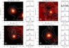 |
Fig. B.1 Leftpanels: false-colour Herschel/PACS images at 70 μm overlaid by the CO (6–5) emission contours towards the TOP100 source. The CO contours correspond to the emission integrated over the full-width at zero power (FWZP) of the CO (6–5) profile, the velocity range shown in the bottom right side of the image, and the contour levels are shown from 20% to 90% of the peak emission of each map, in steps of 10%. The (0,0) position of the map is shown as a + symbol, the position of the CSC source from Contreras et al. (2013) is shown as a × symbol and the dust continuum emission peaks from Csengeri et al. (2014) are shown as asterisks. Right, from top to bottom panel: C17O (2–1) or C18 O (1–0) from Giannetti et al. (2014), CO (4–3), CO (6–5) and CO (7–6) profiles towards the TOP100 sample, convolved into a fixed beam size of 13.′′4 (shown in black) and their fitted Gaussian components. The narrower Gaussian component fitted to the data is shown in blue, the second and broader component is shown in green and the third componentis shown in yellow. The sum of all Gaussian components is shown in red, except for the cases where a single component was fitted. The vertical dashed black line is placed at the rest velocity (Vlsr) of each source. The horizontal filled grey line displays the baseline of the data. |
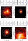 |
Fig. B.1 continued. |
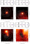 |
Fig. B.1 continued. |
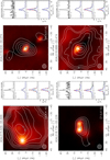 |
Fig. B.1 continued. |
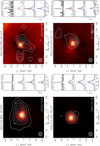 |
Fig. B.1 continued. |
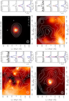 |
Fig. B.1 continued. |
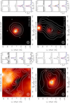 |
Fig. B.1 continued. |
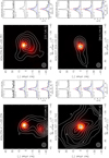 |
Fig. B.1 continued. |
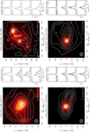 |
Fig. B.1 continued. |
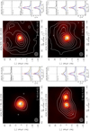 |
Fig. B.1 continued. |
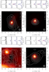 |
Fig. B.1 continued. |
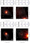 |
Fig. B.1 continued. |
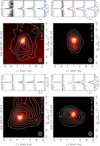 |
Fig. B.1 continued. |
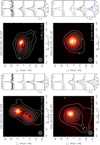 |
Fig. B.1 continued. |
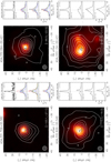 |
Fig. B.1 continued. |
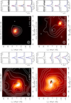 |
Fig. B.1 continued. |
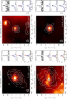 |
Fig. B.1 continued. |
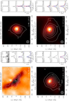 |
Fig. B.1 continued. |
 |
Fig. B.1 continued. |
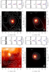 |
Fig. B.1 continued. |
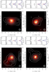 |
Fig. B.1 continued. |
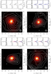 |
Fig. B.1 continued. |
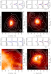 |
Fig. B.1 continued. |
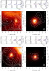 |
Fig. B.1 continued. |
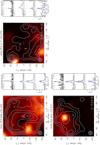 |
Fig. B.1 continued. |
Appendix C Additional material
C.1 Analysis of the mid-J CO emission in the distance-limited sub-sample
For completeness, in this section we present the analysis of the CO emission for the distance-limited sample (defined in Sect. 3.3).
Figure C.1 shows the average CO spectra per class integrated over a linear scale (~0.24 pc) for the distance-limited sub-sample. When compared to Fig. 6, which shows the same kind of spectra but for the full sample (using the spectra convolved to 13.′′ 4, see Sect. 3.3), we found that the IRw and IRb classes are much better separated in the distance-limited sample than in the full dataset smoothed to 13.′′ 4. In fact, the IRw and IRb gets less distinguishable when including the outlier IRw clumps located at d ≥ 12 kpc (AGAL018.606−00.074, AGAL018.734−00.226, AGAL342.484+00.182).
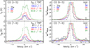 |
Fig. C.1 Leftpanels: average CO (6–5) and CO (7–6) spectra of each ATLASGAL class scaled to the median distance of the distance-limited sub-sample (d = 3.26 kpc). Right panels: same plot, but the average CO spectra were normalised by their peak intensity. The baseline level is indicated by the solid grey line. The black dashed line marks a velocity of 0 km s −1. The FWZP of the profiles are shown in the upper right side of the panels (in km s −1 units), together with the integrated intensity (Sint, in K kms−1 units) of theCO profiles shown in the left panels. |
Figure C.2 presents the CDF for CO (6–5) and CO (7–6) line luminosity. LCO ranges from 2.7 to 284.0 K km s−1 pc2 for the CO (6–5) transition, and 1.2 to 276.5 K km s−1 pc2 for the CO (7–6) line. The KS tests indicate that the evolutionary classes are relatively more distinguishable based on the distance-limited sub-sample than on the full sample (excluding the comparison between IRw and IRb, all tests indicated ranks KS ≥ 0.51, with p ≤ 0.001 for both J transitions, see Table C.1).
Kolmogorov–Smirnov statistics of the mid-J CO line luminosity for the distance-limited sub-sample as a function of the evolutionary class of the clumps.
We also looked at the CO (6–5) and CO (7–6) line luminosities as function of the bolometric luminosity of the sources (see right panel of Fig. C.2), their mass and their luminosity-to-mass ratio (See Fig. C.3). Table C.2 lists the Spearman correlation factor, ρ, and its associated probability, p, for the CO line luminosity versus the bolometric luminosity, the clump mass and the luminosity-to-mass ratio of the clumps. For Lbol and Mclump, the partial Spearman rank, excluding the dependency on the distance, is also provided. The ρ values are similar to those reported on Table 8 for the correlation between LCO and Lbol, based on the 13.′′4 dataset, indicating no significant improvement on the correlation between these quantities. The correlation with Mclump, however, is weaker (ρ ≤ 0.44, p < 0.001) than the one found towards the 13.′′4 dataset (ρ ≥ 0.72, p < 0.001, see Table 8). The weaker correlation between LCO and Mclump on the distance-limited sub-sample might arise from the fact that the CO line luminosity is integrated over only a fraction of the beam used for estimating the mass of the clumps. Indeed König et al. (2017) used a minimum aperture size of 55.′′ 1 for their study, while the minimum beam size adopted for the convolution of the CO was about 10′′ (see Sect. 3.3).
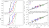 |
Fig. C.2 Left panels: cumulative distribution function (CDF) of the CO line luminosity derived using the spectra convolved to the same linear scale of 0.24 pc. The median values per class are shown as vertical dashed lines in their corresponding colours. Right panels: line luminosity of the same CO lines versus the bolometric luminosity of the TOP100 clumps in distance-limited sub-sample. The median values for each class are shown as open diamonds and their errorbars correspond to the absolute deviation of the data from their median value. Points having an upward arrow indicate a self-absorption feature in the spectrum and correspond to a lower limit. The typical error bars are shown in the bottom right side of the plots. The black solid line is the best fit, the light grey shaded area indicates the 68% uncertainty, and the dashed lines show the intrinsic scatter (ϵ) of the relation. |
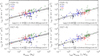 |
Fig. C.3 The CO line luminosity derived using the spectra convolved to the same linear scale of 0.24 pc are shown versus their masses(left panels) and their luminosity-to-mass ratios (right panels). For a complete description of the plots, see Fig. C.2. |
Spearman rank correlation statistics for the CO line luminosity as a function of the clump properties towards the distance-limited sub-sample.
We also found that LCO is relatively better correlated with L∕M for the distance-limited dataset (ρ ≥ 0.67, p < 0.001 for all lines, see Table C.2) rather than the 13.′′ 4 spectra (ρ ≤ 0.50, p ≤ 0.003 for the mid-J CO lines, see Table 8).
We compared the best fits obtained for the mid-J CO line luminosity convolved to the same linear scale with those derived using the 13.′′ 4 data. Table C.3 reports the coefficients of the individual fits. We find that LCO vs. Lbol follows a power-law distribution with indices of 0.53 ± 0.03 and 0.59 ± 0.03 for the CO (6–5) and CO (7–6) lines, respectively. Such power-law distributions are relatively less steeper than those derived towards the 13.′′ 4 dataset, with indices of 0.61 ± 0.03 and 0.67 ± 0.03 for the same J transitions (see Table 7). The offset of the fits indicates the brightness of the CO emission is roughly 0.4 dex larger than the
Parameters of the fits of LCO, extracted within a common linear scale, as a function of the clump properties.
LCO values derived using the spectra convolved toa 13.′′4 beam. At least for the closest sources, such an increment in LCO is expected due to the larger size of the beam corresponding to 0.24 pc. For example, at d = 1.85 kpc, the linear scale of 0.24 pc corresponds to a beam of 26.′′8, which is sampling an area 4 times larger than the 13.′′4 dataset.
Finally, we further investigated the effects of beam dilution on our results by integrating the CO emission over the full maps for those clumps where the aperture used by König et al. (2017) to derive the bolometric luminosity of the clumps, Δθap, was larger or equal to the CO emission extension (Δθ ≤Δθap). Such criterion was satisfied for 92 of the 99 clumps. The best fit of the data indicates that LCO increases with Lbol with a power-law index of 0.59± 0.03 and 0.68  for the CO (6–5) and CO (7–6) transitions, consistently with the results based on the 13.′′ 4 dataset (seeFig. 7). Similar results are also found when comparing LCO versus Mclump and L∕M. The overall results suggests that the analysis of the mid-J CO emission is robust in terms of beam dilution effects.
C.2 Analysis of the CO emission using the Gaussian profiles
We further investigated the effects of self-absorption by computing the CO line luminosities using the integrated flux over the Gaussian fit of the CO profiles (see Sect 3.5). Then, we compared the Gaussian CO luminosities with the clump properties and compared the results with those reported in Sect. 4.3.
First, we checked the correlation between the Gaussian LCO values and the clump properties by means of their Spearman rank correlation factor. The results are summarised in Table C.5. when compared to the Spearman factors of the observed CO line luminosity against the clump properties (see Table 8), we found a slightly improvement on the correlation between LCO and the bolometric luminosity of the clumps (e.g. for the CO (6–5) line, the correlation slightly improves from ρ = 0.85 to 0.88), and with their L∕M ratio (e.g. from ρ = 0.46 to 0.49 for the same transition). No significant changes in the correlation between LCO and Mclump were found (e.g. from ρ = 0.72 to 0.74 for the CO (6–5) line), indicating that the observed correlation is likely dependent on the distance rather than the mass of the clumps.
Spearman statistics for the CO line luminosity as a function of the clump properties using the spectra integrated on the whole CHAMP+ maps.
Spearman rank correlation statistics for the CO line luminosity as a function of the clump properties towards the TOP100 sample for the observed and the Gaussian CO luminosities.
Figure C.4 presents the distribution of the Gaussian CO line luminosities as a function of the clump properties. The parameters of the fits are summarised in Table C.6. Although the distribution of the points indicates higher correlation with Lbol and L∕M, the steepness of the relations are consistent with those reported in Sect. 4.3. For example, the slope of the best fit of LCO against Lbol is 0.63 ± 0.04 for the observed LCO values, and 0.62 ± 0.04 for the Gaussian CO luminosities, respectively. These findings suggests that the relations between the CO line luminosities and the clump properties are robust in terms of the self-absorption observed in the CO spectra of the TOP100.
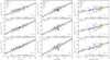 |
Fig. C.4 Line luminosity of the CO (4–3) (upper panels), CO (6–5) (middle panels) and CO (7–6) emission (bottom panels) versus the bolometric luminosity (left panels), the mass of the clumps (middle panels) and the L∕M ratio (right panels) of the TOP100 sources. The median values for each class are shown as open diamonds and their error bars correspond to the absolute deviation of the data from their median value. Points having an upward arrow indicate a self-absorption feature in the spectrum convolved to 13.′′ 4 and correspond to a lower limit. The typical error bars are shown at the bottom right side of the plots. The black solid line is the best fit, the light grey shaded area indicates the 68% uncertainty, and the dashed lines show the intrinsic scatter (ϵ) of the relation. |
Parameters of the fits of LCO as a function of the clump properties for the Gaussian fluxes.
C.3 Integrated CO intensity maps of the secondary Gaussian components
Figure C.5 presents the 870 μm LABOCA maps towards five TOP100 clumps displaying secondary CO peaks in their spectra. The integrated CO (6–5) distribution of the two velocity components clearly shows that the two components trace different structures in the observed field.
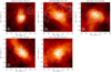 |
Fig. C.5 APEX-LABOCA images at 870 μm overlaid by the CO (6–5) emission contours (C1 component in white, C2 component in black; in both cases, the contours are from 30% to 90% of the peak emission of the corresponding component in steps of 10%) towards the TOP100 clumps. The position of the CSC source from Contreras et al. (2013) is shown as a × symbol. |
References
- Benz, A. O., Bruderer, S., van Dishoeck, E. F., et al. 2016, A&A, 590, A105 [NASA ADS] [CrossRef] [EDP Sciences] [Google Scholar]
- Bergin, E. A., & Tafalla, M. 2007, ARA&A, 45, 339 [NASA ADS] [CrossRef] [Google Scholar]
- Beuther, H., Walsh, A., Schilke, P., et al. 2002, A&A, 390, 289 [NASA ADS] [CrossRef] [EDP Sciences] [Google Scholar]
- Carey, S. J., Noriega-Crespo, A., Mizuno, D. R., et al. 2009, PASP, 121, 76 [NASA ADS] [CrossRef] [Google Scholar]
- Cesaroni, R., Pestalozzi, M., Beltrán, M. T., et al. 2015, A&A, 579, A71 [NASA ADS] [CrossRef] [EDP Sciences] [Google Scholar]
- Cesaroni, R., Sánchez-Monge, Á., Beltrán, M. T., et al. 2016, A&A, 588, L5 [NASA ADS] [CrossRef] [EDP Sciences] [Google Scholar]
- Contreras, Y., Schuller, F., Urquhart, J. S., et al. 2013, A&A, 549, A45 [NASA ADS] [CrossRef] [EDP Sciences] [Google Scholar]
- Csengeri, T., Urquhart, J. S., Schuller, F., et al. 2014, A&A, 565, A75 [NASA ADS] [CrossRef] [EDP Sciences] [Google Scholar]
- Csengeri, T., Leurini, S., Wyrowski, F., et al. 2016, A&A, 586, A149 endrefcommentnewpage [NASA ADS] [CrossRef] [EDP Sciences] [Google Scholar]
- Cubick, M., Stutzki, J., Ossenkopf, V., Kramer, C., & Röllig, M. 2008, A&A, 488, 623 [NASA ADS] [CrossRef] [EDP Sciences] [Google Scholar]
- de Graauw, T., Helmich, F. P., Phillips, T. G., et al. 2010, A&A, 518, L6 [NASA ADS] [CrossRef] [EDP Sciences] [Google Scholar]
- Decarli, R., Walter, F., Aravena, M., et al. 2016, ApJ, 833, 70 [NASA ADS] [CrossRef] [Google Scholar]
- Faúndez, S., Bronfman, L., Garay, G., et al. 2004, A&A, 426, 97 [NASA ADS] [CrossRef] [EDP Sciences] [Google Scholar]
- Giannetti, A., Wyrowski, F., Brand, J., et al. 2014, A&A, 570, A65 [NASA ADS] [CrossRef] [EDP Sciences] [Google Scholar]
- Giannetti, A., Leurini, S., Wyrowski, F., et al. 2017, A&A, 603, A33 [NASA ADS] [CrossRef] [EDP Sciences] [Google Scholar]
- Gómez-Ruiz, A. I., Gusdorf, A., Leurini, S., et al. 2012, A&A, 542, L9 [NASA ADS] [CrossRef] [EDP Sciences] [Google Scholar]
- Grellmann, R., Preibisch, T., Ratzka, T., et al. 2013, A&A, 550, A82 [NASA ADS] [CrossRef] [EDP Sciences] [Google Scholar]
- Güsten, R., Nyman, L. Å., Schilke, P., et al. 2006, A&A, 454, L13 [NASA ADS] [CrossRef] [EDP Sciences] [Google Scholar]
- Güsten, R., Baryshev, A., Bell, A., et al. 2008, in SPIE Conf. Ser., 7020, 10 [Google Scholar]
- Hosokawa, T., & Omukai, K. 2009, ApJ, 691, 823 [NASA ADS] [CrossRef] [Google Scholar]
- Karska, A., Herpin, F., Bruderer, S., et al. 2014, A&A, 562, A45 [NASA ADS] [CrossRef] [EDP Sciences] [Google Scholar]
- Kasemann, C., Güsten, R., Heyminck, S., et al. 2006, in SPIE Conf. Ser., 6275, 0 [Google Scholar]
- Kim, W.-J., Wyrowski, F., Urquhart, J. S., Menten, K. M., & Csengeri, T. 2017, A&A, 602, A37 [NASA ADS] [CrossRef] [EDP Sciences] [Google Scholar]
- Klein, T., Ciechanowicz, M., Leinz, C., et al. 2014, IEEE Trans. Terahertz Sci. Technol., 4, 588 [NASA ADS] [CrossRef] [Google Scholar]
- König, C., Urquhart, J. S., Csengeri, T., et al. 2017, A&A, 599, A139 [NASA ADS] [CrossRef] [EDP Sciences] [Google Scholar]
- Krumholz, M. R., Klein, R. I., McKee, C. F., Offner, S. S. R., & Cunningham, A. J. 2009, Science, 323, 754 [NASA ADS] [CrossRef] [PubMed] [Google Scholar]
- Leurini, S., Wyrowski, F., Herpin, F., et al. 2013, A&A, 550, A10 [NASA ADS] [CrossRef] [EDP Sciences] [Google Scholar]
- Leurini, S., Codella, C., López-Sepulcre, A., et al. 2014, A&A, 570, A49 [NASA ADS] [CrossRef] [EDP Sciences] [Google Scholar]
- Leurini, S., Wyrowski, F., Wiesemeyer, H., et al. 2015, A&A, 584, A70 [NASA ADS] [CrossRef] [EDP Sciences] [Google Scholar]
- Molinari, S., Pezzuto, S., Cesaroni, R., et al. 2008, A&A, 481, 345 [NASA ADS] [CrossRef] [EDP Sciences] [Google Scholar]
- Molinari, S., Swinyard, B., Bally, J., et al. 2010, PASP, 122, 314 [NASA ADS] [CrossRef] [Google Scholar]
- Molinari, S., Schisano, E., Elia, D., et al. 2016, A&A, 591, A149 [NASA ADS] [CrossRef] [EDP Sciences] [Google Scholar]
- Mottram, J. C., van Dishoeck, E. F., Kristensen, L. E., et al. 2017, A&A, 600, A99 [NASA ADS] [CrossRef] [EDP Sciences] [Google Scholar]
- Rosen, A. L., Krumholz, M. R., McKee, C. F., & Klein, R. I. 2016, MNRAS, 463, 2553 [NASA ADS] [CrossRef] [Google Scholar]
- San José-García, I., Mottram, J. C., Kristensen, L. E., et al. 2013, A&A, 553, A125 [NASA ADS] [CrossRef] [EDP Sciences] [Google Scholar]
- San José-García, I., Mottram, J. C., van Dishoeck, E. F., et al. 2016, A&A, 585, A103 [NASA ADS] [CrossRef] [EDP Sciences] [Google Scholar]
- Saraceno, P., Andre, P., Ceccarelli, C., Griffin, M., & Molinari, S. 1996, A&A, 309, 827 [NASA ADS] [Google Scholar]
- Schuller, F., Menten, K. M., Contreras, Y., et al. 2009, A&A, 504, 415 [NASA ADS] [CrossRef] [EDP Sciences] [Google Scholar]
- Schulz, A., Henkel, C., Beckmann, U., et al. 1995, A&A, 295, 183 [NASA ADS] [Google Scholar]
- Tang, X. D., Henkel, C., Wyrowski, F., et al. 2018, A&A, 611, A6 [NASA ADS] [CrossRef] [EDP Sciences] [Google Scholar]
- Urquhart, J. S., Moore, T. J. T., Schuller, F., et al. 2013a, MNRAS, 431, 1752 [Google Scholar]
- Urquhart, J. S., Thompson, M. A., Moore, T. J. T., et al. 2013b, MNRAS, 435, 400 [NASA ADS] [CrossRef] [Google Scholar]
- Urquhart, J. S., König, C., Giannetti, A., et al. 2018, MNRAS, 473, 1059 [NASA ADS] [CrossRef] [Google Scholar]
- van Kempen, T. A., van Dishoeck, E. F., Güsten, R., et al. 2009a, A&A, 507, 1425 [NASA ADS] [CrossRef] [EDP Sciences] [Google Scholar]
- van Kempen, T. A., van Dishoeck, E. F., Hogerheijde, M. R., & Güsten, R. 2009b, A&A, 508, 259 [Google Scholar]
- van Kempen, T. A., Kristensen, L. E., Herczeg, G. J., et al. 2010, A&A, 518, L121 [NASA ADS] [CrossRef] [EDP Sciences] [Google Scholar]
- Weiß, A., Downes, D., Neri, R., et al. 2007, A&A, 467, 955 [NASA ADS] [CrossRef] [EDP Sciences] [Google Scholar]
- Wienen, M., Wyrowski, F., Schuller, F., et al. 2012, A&A, 544, A146 [NASA ADS] [CrossRef] [EDP Sciences] [Google Scholar]
- Wu, J., Evans, II, N. J., Gao, Y., et al. 2005, ApJ, 635, L173 [NASA ADS] [CrossRef] [Google Scholar]
- Yorke, H. W.,& Bodenheimer, P. 1999, ApJ, 525, 330 [NASA ADS] [CrossRef] [Google Scholar]
- Zhang, X., Lee, Y., Bolatto, A., & Stark, A. A. 2001, ApJ, 553, 274 [NASA ADS] [CrossRef] [Google Scholar]
- Zinnecker, H., & Yorke, H. W. 2007, ARA&A, 45, 481 [NASA ADS] [CrossRef] [Google Scholar]
Based on observations with the APEX telescope under programme IDs M-087.F-0030-2011, M-093.F-0026-2014 and M-096.F-0005-2015. APEX is a collaboration between the Max-Planck-Institut für Radioastronomie, the European Southern Observatory, and the Onsala Space Observatory.
All Tables
Results of the Gaussian fit of the CO spectra convolved to a common angular resolution of 13.′′ 4.
Statistics of the FWHM of the Gaussian components fitted on the CO line profiles convolved to a common angular resolution of 13.′′4.
Statistics on the CO line profiles, convolved to a common angular resolution of 13.′′ 4.
Kolmogorov–Smirnov statistics of the CO line luminosity as a function of the evolutionary class of the clumps.
Spearman rank correlation statistics for the CO line luminosity as a function of the clump properties towards the TOP100 sample.
Parameters of the fits of LCO as a function of the clump properties for the TOP100 clumps that are not affected by self-absorption features.
Spearman rank correlation statistics for the CO line luminosity as a function of the clump properties for the TOP100 clumps that are not affected by self-absorption features.
Kolmogorov–Smirnov statistics of the excitation temperature of the CO (6–5) line as a function of the evolutionary class of the clumps.
Kolmogorov–Smirnov statistics of the mid-J CO line luminosity for the distance-limited sub-sample as a function of the evolutionary class of the clumps.
Spearman rank correlation statistics for the CO line luminosity as a function of the clump properties towards the distance-limited sub-sample.
Parameters of the fits of LCO, extracted within a common linear scale, as a function of the clump properties.
Spearman statistics for the CO line luminosity as a function of the clump properties using the spectra integrated on the whole CHAMP+ maps.
Spearman rank correlation statistics for the CO line luminosity as a function of the clump properties towards the TOP100 sample for the observed and the Gaussian CO luminosities.
Parameters of the fits of LCO as a function of the clump properties for the Gaussian fluxes.
All Figures
|
Fig. 1 Ratio between the daily integrated flux and the average flux of the CO (6–5) transition for the calibration sources observed during the campaign. A solid horizontal line is placed at 1.0 and the dashed lines indicate a deviation of 20% from unity. |
| In the text | |
|
Fig. 2 Gaussian decomposition for the CO (6–5) line using up to 3 components. Panel A: single Gaussian fit; panel B: two-components fit; panel C: two-components fit (channels affected by self absorption are masked); panel D: three-components fit (channels affected by self absorption are masked). The spectra, fits and residuals were multiplied by the factor shown in each panel. The Gaussian fits are shown in blue, green and yellow, ordered by their line width; the sum of all components is shown in red. The grey lines indicate the baseline and the dashed horizontal lines placed in the residuals correspond to the 3-σ level. Self-absorption features larger than 5-σ were masked out from the residuals. |
| In the text | |
|
Fig. 3 Distribution of the CO (6–5) emission of four representative clumps of each evolutionary classes of the TOP100 clumps. The CO contours are presented on top of the Herschel-PACS maps at 70 μm. Each 70 μm map is scaled in according to the colour bar shown in the corresponding panel. The CO contours correspond to the emission integrated over the full-width at zero power (FWZP) of the CO (6–5) line, andthe contour levels are shown from 20% to 90% of the peak emission of each map, in steps of 10%. The position of the CSC source from Contreras et al. (2013) is shown as a × symbol. Thebeam size of the CO (6–5) observations is indicated in the left bottom region. |
| In the text | |
|
Fig. 4 Size ofthe CO (6–5) emission towards the TOP100 sample versus the bolometric luminosity (top panel) and the mass (bottom panel) of the sources. The median values for each class are shown as open diamonds and their error bars correspond to the absolute deviation of the data from their median value. The typical uncertainty is shown by the error bars on the bottom right of each plot. |
| In the text | |
|
Fig. 5 Size of the CO (6–5) emission versus the size of the 70 μm emission from the Herschel-PACS images towards the 70 μm-bright clumps. The dashed line indicates y = x. The median values for the 70 μm-bright classes are shown as open diamonds and their error bars correspond to the absolute deviation of the data from their median value. The typical uncertainty, computed as the dispersion between the major and minor axis of the emission, is shown by the error bars on the bottom right of each plot. |
| In the text | |
|
Fig. 6 Left panels: average CO (4–3), CO (6–5) and CO (7–6) spectra convolved to 13.′′ 4 beam of each evolutionary class scaled to the median distance of the whole sample (d = 3.80 kpc). Right panels: same plot, but the average CO spectra are normalised by their peak intensity. The baseline level is indicated by the solid grey line and the black dashed line is placed at 0 km s−1. The FWZP of the profiles are shown in the upper right side of the panels (in km s −1 units), together with the integrated intensities (Sint, in K kms−1 units) of theCO profiles shown in the left panels. |
| In the text | |
|
Fig. 7 Left panels: cumulative distribution function of the line luminosity of the CO (4–3) (upper panel), CO (6–5) (middle panel) and CO (7–6) emission (bottom panel) towards the TOP100 sample. The median values per class are shown as vertical dashed lines in their corresponding colours. Right panels: Line luminosity of the same CO J-transitions versus the bolometric luminosity of the TOP100 sources. The median values for each class are shown as open diamonds and their error bars correspond to the absolute deviation of the data from their median value. Data points highlighted in yellow indicate those sources from which no signs of self-absorption features where identified in the spectrum convolved to 13.′′ 4. The typical error bars are shown at the bottom right side of the plots. The black solid line is the best fit, the light grey shaded area indicates the 68% uncertainty, and the dashed lines show the intrinsic scatter (ϵ) of the relation. |
| In the text | |
|
Fig. 8 Same as the right panel of Fig. 7, but displaying the line luminosity of the CO (6–5) emission as a function of the mass of the clumps. Data points highlighted in yellow indicate those sources from which no signs of self-absorption features where identified in the spectrum convolved to 13.′′ 4. |
| In the text | |
|
Fig. 9 Same as the right panel of Fig. 7, but displaying LCO of the CO (6–5) line as a function of the L∕M ratio of the TOP100 sources. Data points highlighted in yellow indicate those sources from which no signs of self-absorption features where identified in the spectrum convolved to 13.′′ 4. |
| In the text | |
|
Fig. 10 Excitation temperature of the CO (6–5) line versus the bolometric luminosity of the TOP100 clumps (left panels) and the luminosity-to-mass ratio (right panels). The excitation temperature was derived using the peak of the Gaussian fit of the CO profiles. The median values for each class are shown as open diamonds and their error bars correspond to the median absolute deviation of the data from their median value. The black solid line is the best fit, the light grey shaded area indicates the 68% uncertainty, and the dashed lines show the intrinsic scatter (ϵ) of the relation. The best fit to the data is indicated by the filled black line. |
| In the text | |
|
Fig. 11 Power-law indices of the LCO versus Lbol relations for different J transitions as a function of the upper-level J number. Theβ indices from Table 7 (filled black circles) are plotted together with data from SJG13 (open grey circle, excluded from the fit) and the exponent derived for their high-luminosity sub-sample (* symbol, see Fig. 12). The best fit is indicated by the dashed black line. |
| In the text | |
|
Fig. 12 CO line luminosity as a function of the bolometric luminosity for the CO (6–5) (upper panel), CO (7–6) (middle panel) and CO (10–9) (bottom panel) transitions. The fits were performed on the whole dataset (all points, shown with black contours), on the low- and high-luminosity sub-samples (points filled in red and blue, respectively). The CO (6–5) and CO (7–6) data towards low-luminosity sources are from van Kempen et al. (2009a); the CO (10–9) data are from San José-García et al. (2013). The dashed vertical line at Lbol = 50 L⊙ marks the transition from low- to high-mass YSOs. The typical error bars are shown in the bottom right side of the plots. |
| In the text | |
|
Fig. B.1 Leftpanels: false-colour Herschel/PACS images at 70 μm overlaid by the CO (6–5) emission contours towards the TOP100 source. The CO contours correspond to the emission integrated over the full-width at zero power (FWZP) of the CO (6–5) profile, the velocity range shown in the bottom right side of the image, and the contour levels are shown from 20% to 90% of the peak emission of each map, in steps of 10%. The (0,0) position of the map is shown as a + symbol, the position of the CSC source from Contreras et al. (2013) is shown as a × symbol and the dust continuum emission peaks from Csengeri et al. (2014) are shown as asterisks. Right, from top to bottom panel: C17O (2–1) or C18 O (1–0) from Giannetti et al. (2014), CO (4–3), CO (6–5) and CO (7–6) profiles towards the TOP100 sample, convolved into a fixed beam size of 13.′′4 (shown in black) and their fitted Gaussian components. The narrower Gaussian component fitted to the data is shown in blue, the second and broader component is shown in green and the third componentis shown in yellow. The sum of all Gaussian components is shown in red, except for the cases where a single component was fitted. The vertical dashed black line is placed at the rest velocity (Vlsr) of each source. The horizontal filled grey line displays the baseline of the data. |
| In the text | |
|
Fig. B.1 continued. |
| In the text | |
|
Fig. B.1 continued. |
| In the text | |
|
Fig. B.1 continued. |
| In the text | |
|
Fig. B.1 continued. |
| In the text | |
|
Fig. B.1 continued. |
| In the text | |
|
Fig. B.1 continued. |
| In the text | |
|
Fig. B.1 continued. |
| In the text | |
|
Fig. B.1 continued. |
| In the text | |
|
Fig. B.1 continued. |
| In the text | |
|
Fig. B.1 continued. |
| In the text | |
|
Fig. B.1 continued. |
| In the text | |
|
Fig. B.1 continued. |
| In the text | |
|
Fig. B.1 continued. |
| In the text | |
|
Fig. B.1 continued. |
| In the text | |
|
Fig. B.1 continued. |
| In the text | |
|
Fig. B.1 continued. |
| In the text | |
|
Fig. B.1 continued. |
| In the text | |
|
Fig. B.1 continued. |
| In the text | |
|
Fig. B.1 continued. |
| In the text | |
|
Fig. B.1 continued. |
| In the text | |
|
Fig. B.1 continued. |
| In the text | |
|
Fig. B.1 continued. |
| In the text | |
|
Fig. B.1 continued. |
| In the text | |
|
Fig. B.1 continued. |
| In the text | |
|
Fig. C.1 Leftpanels: average CO (6–5) and CO (7–6) spectra of each ATLASGAL class scaled to the median distance of the distance-limited sub-sample (d = 3.26 kpc). Right panels: same plot, but the average CO spectra were normalised by their peak intensity. The baseline level is indicated by the solid grey line. The black dashed line marks a velocity of 0 km s −1. The FWZP of the profiles are shown in the upper right side of the panels (in km s −1 units), together with the integrated intensity (Sint, in K kms−1 units) of theCO profiles shown in the left panels. |
| In the text | |
|
Fig. C.2 Left panels: cumulative distribution function (CDF) of the CO line luminosity derived using the spectra convolved to the same linear scale of 0.24 pc. The median values per class are shown as vertical dashed lines in their corresponding colours. Right panels: line luminosity of the same CO lines versus the bolometric luminosity of the TOP100 clumps in distance-limited sub-sample. The median values for each class are shown as open diamonds and their errorbars correspond to the absolute deviation of the data from their median value. Points having an upward arrow indicate a self-absorption feature in the spectrum and correspond to a lower limit. The typical error bars are shown in the bottom right side of the plots. The black solid line is the best fit, the light grey shaded area indicates the 68% uncertainty, and the dashed lines show the intrinsic scatter (ϵ) of the relation. |
| In the text | |
|
Fig. C.3 The CO line luminosity derived using the spectra convolved to the same linear scale of 0.24 pc are shown versus their masses(left panels) and their luminosity-to-mass ratios (right panels). For a complete description of the plots, see Fig. C.2. |
| In the text | |
|
Fig. C.4 Line luminosity of the CO (4–3) (upper panels), CO (6–5) (middle panels) and CO (7–6) emission (bottom panels) versus the bolometric luminosity (left panels), the mass of the clumps (middle panels) and the L∕M ratio (right panels) of the TOP100 sources. The median values for each class are shown as open diamonds and their error bars correspond to the absolute deviation of the data from their median value. Points having an upward arrow indicate a self-absorption feature in the spectrum convolved to 13.′′ 4 and correspond to a lower limit. The typical error bars are shown at the bottom right side of the plots. The black solid line is the best fit, the light grey shaded area indicates the 68% uncertainty, and the dashed lines show the intrinsic scatter (ϵ) of the relation. |
| In the text | |
|
Fig. C.5 APEX-LABOCA images at 870 μm overlaid by the CO (6–5) emission contours (C1 component in white, C2 component in black; in both cases, the contours are from 30% to 90% of the peak emission of the corresponding component in steps of 10%) towards the TOP100 clumps. The position of the CSC source from Contreras et al. (2013) is shown as a × symbol. |
| In the text | |
Current usage metrics show cumulative count of Article Views (full-text article views including HTML views, PDF and ePub downloads, according to the available data) and Abstracts Views on Vision4Press platform.
Data correspond to usage on the plateform after 2015. The current usage metrics is available 48-96 hours after online publication and is updated daily on week days.
Initial download of the metrics may take a while.