| Issue |
A&A
Volume 618, October 2018
|
|
|---|---|---|
| Article Number | A6 | |
| Number of page(s) | 15 | |
| Section | Extragalactic astronomy | |
| DOI | https://doi.org/10.1051/0004-6361/201832790 | |
| Published online | 03 October 2018 | |
Spatially resolved electron density in the narrow line region of z < 0.02 radio AGNs
1 European Southern Observatory, Karl-Schwarzschild-Str. 2, 85748 Garching bei München, Germany
e-mail: This email address is being protected from spambots. You need JavaScript enabled to view it.
2 Ludwig-Maximilian-Universität, Professor-Huber-Platz 2, 80539 München, Germany
3 European Southern Observatory, Alonso de Cordova 3107, Vitacura, Casilla 19001, Santiago de Chile, Chile
4 Research School for Astronomy & Astrophysics, Australian National University, Cotter Road, Weston Creek, ACT 2611, Australia
5 ARC Center of Excellence for All Sky Astrophysics in 3 Dimensions (ASTRO 3D), Australia
6 Max-Planck-Institut für Extraterrestrische Physik, Giessenbachstrasse, 85748 Garching, Germany
7 National Centre for Radio Astrophysics, Tata Institute of Fundamental Research, S. P. Pune University Campus, Post Bag 3, Ganeshkhind, Pune 411007, India
8 Gemini Observatory, Northern Operations Center, 670 N. A’ohoku Pl., Hilo, HI 96720, USA
9 Max Planck Institute for Astronomy, Königstuhl, 17, 69117 Heidelberg, Germany
Received:
7
February
2018
Accepted:
6
June
2018
Abstract
Context. Although studying outflows in the host galaxies of active galactic nuclei (AGNs) have moved to the forefront of extragalactic astronomy in recent years, estimating the energy associated with these outflows has been a major challenge. Determining the energy associated with an outflow often involves an assumption of uniform density in the narrow line region (NLR), which spans a wide range in the literature, leading to large systematic uncertainties in energy estimation.
Aims. In this paper we present electron density maps for a sample of outflowing and non-outflowing Seyfert galaxies at z < 0.02 drawn from the Siding Spring Southern Seyfert Spectroscopic Snapshot Survey (S7) and try to understand the origin and values of the observed density structures to reduce the systematic uncertainties in outflow energy estimation.
Methods. We use the ratio of the [S II]λ6716,6731 emission lines to derive spatially resolved electron densities (≲50–2000 cm−3). Using optical Integral Field Unit observations from the Wide Field Spectrograph (WiFeS), we are able to measure densities across the central 2–5 kpc of the selected AGN host galaxies. We compare the density maps with the positions of the H II regions derived from the narrow Hα component, ionization maps from [O III] and spatially resolved BPT diagrams to infer the origin of the observed density structures. We also use the electron density maps to construct density profiles as a function of distance from the central AGN.
Results. We find a spatial correlation between the sites of high star formation and high electron density for targets without an active ionized outflow. The non-outflowing targets also show an exponential drop in the electron density as a function of distance from the centre, with a mean exponential index of ∼0.15. The correlation between the star forming sites and electron density ceases for targets with an outflow. The density within the outflowing medium is not uniform and shows both low- and high-density sites, most likely due to the presence of shocks and highly turbulent medium. We compare these results in the context of previous results obtained from fibre and slit spectra.
Key words: galaxies: active / galaxies: ISM / galaxies: nuclei
ESO Fellow.
© ESO 2018
1. Introduction
Ionizing radiation from accreting supermassive black holes (SMBH) at the centre of galaxies is believed to illuminate the narrow line regions in the host galaxies of active galactic nuclei (AGN). Unlike the centrally concentrated broad line region (BLR), the narrow line region (NLR) can extend up to kiloparsec scales (e.g. Greene et al. 2012; Sun et al. 2017).
This offers a platform to study the ISM properties of the AGN host galaxies, such as electron density, electron temperature, and the shape of the ionizing radiation field using rest frame optical emission lines arising from the ionized gas (e.g. Kewley & Dopita 2002; Dopita et al. 2006; Bennert et al. 2006a; Kewley et al. 2013; Davies et al. 2017). For low-redshift galaxies the spatial extent means the NLR structure can be resolved, and thus the NLR properties can be studied as a function of distance from the galactic nucleus (e.g. Heckman et al. 1990; Bennert et al. 2006a,b,c).
Outflows in the ionized gas phase in AGN host galaxies are known to exist at both low and high redshift (e.g. Perna et al. 2015a; Villar-Martín et al. 2016; Zakamska et al. 2016; Toba et al. 2017). Calculation of the energy associated with such outflows often requires an assumption of the value of the electron density in the NLR, which is in the range <10–10 000 cm−3 (e.g. Nesvadba et al. 2006; Liu et al. 2013; Harrison et al. 2014). This represents the largest fraction of the systematic uncertainty budget in the outflow energy estimate in the ionized gas phase (e.g. Müller-Sánchez et al. 2011; Kakkad et al. 2016; Perna et al. 2017) and consequently the coupling between the kinetic power of the outflowing gas and the physical properties of the central AGN or star formation remains unclear. This further prevents us from knowing the source of such outflows, i.e. whether they are driven by the AGN itself or by star bursts. Therefore, it is crucial to understand the electron density values in the ISM of an AGN host galaxy and how the presence of an outflow affects it.
Most existing electron density studies in galaxies are based on the optical emission lines [S II]λ6716,6731 (hereafter [S II] doublet) or [O II]λ3726,3729 (hereafter [O II] doublet), as these lines are easily accessible across a wide range of redshifts. Both sets of lines arise from two closely spaced “meta-stable” energy levels, which means that the relative flux values only depend on the electron density occupying these levels and any degeneracy due to different ions is also removed (Osterbrock & Ferland 2006). Although the temperature dependence of electron density is non-negligible, the measurement errors are usually larger than the errors introduced by the temperature assumption (see also Sanders et al. 2016). Due to the small wavelength separation, the use of the [O II] doublet to determine the electron density is limited by the spectral resolution of most of the instruments (including the Wide Field Spectrograph used in this paper, see Sect. 3). Hence, the optical [S II] doublet is more commonly used to measure electron densities. The [S II] doublet is sensitive to densities between ∼50 and 2000 cm−3, within the typically estimated range of densities in the extended NLR (see Sect. 3). Below and above these densities, the flux ratio of the doublet becomes saturated and is hence unreliable.
Investigation of electron densities have been conducted in both star forming and AGN host galaxies in the past decade (e.g. Bennert et al. 2006a; Xu et al. 2007; Hainline et al. 2009; Shirazi et al. 2014; Darvish et al. 2015; Sanders et al. 2016; Perna et al. 2017; Comerford et al. 2017) most of which claim elevated electron densities linked to the higher star formation rates (SFRs, e.g. Shimakawa et al. 2015; Kaasinen et al. 2017), although there have been counter-arguments to this result (e.g. Darvish et al. 2015). Electron density obtained from one-dimensional fibre and two-dimensional slit spectra for high-redshift star forming galaxies show an increase in the density of one order of magnitude compared to the low-redshift studies (e.g. Sanders et al. 2016; Kaasinen et al. 2017). Also, recent studies targeting optically selected AGNs from SDSS (Perna et al. 2017) suggested an enhancement of electron density in the outflowing medium.
However, most of these studies at high redshift (z ∼ 1−2) have the observational limitation in resolving the central and the outer regions of the galaxy. The electron density values for these high-redshift galaxies are based on average density values obtained from integrated spectra using one-dimensional fibre or two-dimensional slit spectroscopy. The central regions of a galaxy are expected to have a higher density than the outer NLR (e.g. Bennert et al. 2006a), and therefore estimation of density from an integrated spectrum has the limitation that they could potentially be contaminated by the higher density nuclear regions of the galaxies.
Galaxies at low redshift, on the other hand, overcome the limitation of low spatial resolution and are thus ideal for performing spatially resolved electron density studies. By combining electron density maps with information from other emission lines such as Hα (tracing current star formation) and [O III] (tracing AGN ionization), we can understand whether and how the density morphology is impacted by star formation or AGN processes or outflows. In this paper we focus on the low-redshift AGN sample.
There are numerous studies which have presented spatial information on electron density in nearby galaxies (e.g. Bennert et al. 2006a; Storchi-Bergmann et al. 2009; Sharp & Bland-Hawthorn 2010; Westmoquette et al. 2011, 2013; Freitas et al. 2018). These studies include a combination of starburst galaxies, AGN hosts, and ultraluminous infrared galaxies (ULIRGs) with a fraction of them hosting fast velocity outflows of ∼1000 km s−1. Bennert et al. (2006a) presented the electron density as a function of radius from the central AGN in a sample of low-redshift Seyfert 1 and Seyfert 2 galaxies using single-slit spectroscopy from FORS1/VLT1 and EMMI/NTT2. It was observed that the density measured using the optical [S II] doublet saturate at the lower limit (<50 cm−3) for distance greater than 500 pc from the central AGN. Although the Bennert et al. (2006a) work was based on targets which did not show the presence of an outflow, the drop in density is supported in targets which show an evident outflow from most of the density maps presented in Sharp & Bland-Hawthorn (2010), Cresci et al. (2015), and Freitas et al. (2018) for instance. Also, the electron densities probed in these maps are consistent with the typical density in the NLR ranging from tens to a few thousand cm−3.
An important addition to these previous works is to determine the density in the outflowing medium, which otherwise is measured from the total flux of the [S II] doublet ratio potentially including contributions from the non-outflowing material. Moreover, it is essential to know whether the density values and morphology change due to the presence of an ionized outflow. To understand the impact of an outflow on the electron density, it is necessary to perform a similar spatially resolved analysis on multiple targets and compare the results for targets with and without an active ionized outflow, which forms the basis of this paper. We note that we refer to the density of the warm ionized gas component which is traced by the optical emission lines as [O III]λ5007 and [S II]. Numerous other tracers for electron density exist, such as transauroral emission lines (Spence et al. 2018) and the FeII doublet (Storchi-Bergmann et al. 2009) which trace a different gas phase and are sensitive to regions with higher density (>104 cm−3).
Today, large samples of optical and near-infrared IFU spectra of extra-galactic sources building up through IFU surveys such as SAMI (Croom et al. 2012), MaNGA (Bundy et al. 2015; Wake et al. 2017), S7 (Dopita et al. 2015; Thomas et al. 2017), KASHz (Harrison et al. 2016), KMOS3D (Wisnioski et al. 2015), and KDS (Turner et al. 2017) allow us to perform such a study on a large sample of galaxies. In this paper we present the electron density distribution for a subsample of low-redshift AGN host galaxies derived from the S7 survey with the aim of deriving their electron density profiles as a function of radius and identifying the mechanisms—Star formation, AGN ionization or outflows—which drive the observed density patterns.
The paper is structured as follows: In Sect. 2, we briefly summarize the properties of the S7 subsample used in this paper, its observations, and data reduction procedures. Section 3 gives a comprehensive overview of the analysis procedures, namely line fitting, map construction, and error estimation. The resulting spectra, star formation and extinction maps, [O III] flux maps, and electron density profiles are given in Sect. 4. We discuss the processes leading to the observed electron density patterns and the implications of these results in Sect. 5. The main conclusions of the paper are presented in Sect. 6.
Throughout this paper, we adopt a Λ-CDM cosmology with H0 = 70 km s−1 Mpc−1, Ωm = 0.3, ΩΛ = 0.7 and Ωr = 0.0.
2. Sample: the Siding Spring Southern Seyfert Spectroscopic Snapshot Survey
Our sample is drawn from the Siding Spring Southern Seyfert Spectroscopic Snapshot Survey (S7, Dopita et al. 2015; Thomas et al. 2017), which is an Integral Field Spectroscopic survey of nearby Seyfert and LINER galaxies at z < 0.02. Here we briefly describe the basic characteristics of this survey. We refer the reader to the data release papers, Dopita et al. (2015) and Thomas et al. (2017), for further details on the sample selection, observing strategy, and object-by-object description of the survey.
The observations for the S7 survey were carried out using the Wide Field Spectrograph (WiFeS) on ANU 2.3 m telescope at the Siding Spring Observatory. The field of view (FOV) is 38 × 25 arcsec2 with the nucleus centred on the field of view and orientation close to the major axis of the galaxy (Fig. 1 shows NGC 1365 as an example). The spectra have a resolution of R = 3000 for 340 <λ< 560 nm and a moderately high spectral resolution of R = 7000 (∼50 km s−1) in the wavelength range 530 <λ< 710 nm (hereafter “blue” and “red” spectra). The average spatial resolution for the observations is ∼1–2 arcsec corresponding to the seeing, with exposure times in the range 800– 1000 s. The data reduction was performed using Python pipeline PYWIFES (Childress et al. 2014), which provides calibrated sky subtracted data cubes resampled on a 1 × 1 arsec2 pixel scale. The error budget on flux calibration is up to 4%. The survey is aimed at probing the ionizing mechanism of the extended narrow line region (ENLR) of nearby radio-selected AGNs with 20 cm radio flux density greater than 20 mJy. Given the redshift distribution of the sample, the spatial resolution of the data is ≲400 pc arcsec−1 and diagnostic lines such as Hβ, [O III]λ5007, Hα,[N II]λ6585, and [S II]λ6716,6731 used in this paper are well within the spectral range of WiFeS. Such a wide range in the coverage of emission lines makes this survey extremely useful; the contribution to these line fluxes due to star formation or AGN or both can be disentangled using spatially resolved diagnostic diagrams.
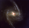 |
Fig. 1. Representation of the field of view (FOV) covered by WiFeS instrument used in the S7 survey. The figure shows a 7 × 7 arcmin2 FORS1/VLT image of NGC 1365, one of the galaxies targeted with the S7 survey, as an example. The WiFeS FOV (38 × 25 arcsec2) is overlaid in red. The S7 FOV for the rest of the targets are presented in Dopita et al. (2015) and Thomas et al. (2017). North is up and east is to left. Image credit: ESO. |
The S7 subsample used in this paper was chosen to cover a wide range in morphology of star forming regions, as traced by the Hα emission line, and NLRs, as traced by the [O III] emission. The sample includes a mixture of Seyfert 1 galaxies, Seyfert 2 galaxies, and AGN-Starburst (SB) composite systems. We also filter out targets in which the [S II] doublet is contaminated by skylines, stellar continuum, and atmospheric absorption features and where the S/N of the [S II] emission line is less than 5; a contamination of the [S II] lines and/or poor data quality can significantly affect the density measurement, as explained in Sect. 3. The 13 targets presented in this paper lie in the low-redshift range of 0.0038–0.0164 which probes a maximum physical scale of ∼5 kpc corresponding to the WiFeS FOV. The average seeing of all the targets used in the paper lies between 1.1–2.2 arcsec, which corresponds to 1–2 pixels. These properties have been summarized in Table 1. This spatial resolution and the FOV allow us to probe the density structures within the AGN host galaxy on scales of ∼100 pc–5 kpc.
Properties of the S7 subsample used in this paper.
Three of the targets, namely NGC 1068, NGC 1266, and NGC 2110, are classified as having an ionized outflow based on the presence of broad components in the [O III]5007 profile of the S7 data. The broad components of the [O III] profiles in the three targets show fast outflows with FWHM > 500 km s−1 compared to the other targets which require only narrow components with FWHM < 200 km s−1 (see Sect. 3.1 for more details on emission line fitting). A number of works in the literature report the presence of outflows in other targets as well. The difference in the classification of the presence of outflows presented in this paper from the previous works may be due to the different aperture probed by the S7 data (the central 35 × 25 arcsec2) and the above-mentioned definition of outflow. Hereafter, we refer to the presence of ionized outflows based on the definition mentioned above as interpreted from the S7 data. This paper focuses on the analysis of the warm ionized gas in the NLR traced by the [O III] line. A comparison of electron density values between the outflowing and non-outflowing targets also helps us infer whether the presence of outflows makes any difference to the density morphology and their values.
3. Data analysis
As described in the introduction, the [S II] doublet and [O II] doublet are ideal tracers of the electron density in a warm ionized medium. The spectral resolution of WiFeS does not allow us to de-blend the [O II] doublet, and so in this paper we measure electron densities using the flux ratio of the [S II] doublet. For the typical range of values of the electron density in the NLR, i.e. <50–2000 cm−3,3 the theoretical [S II] doublet line ratio is close to unity, between 0.7 and 1.45 (Osterbrock & Ferland 2006). Since the inferred electron density is highly influenced by minute changes in the flux ratio, we applied a S/N cut of 5 in the overall spectrum and in the individual pixels of each target during the analysis. The following section provides a detailed description of the analysis tools used in this paper. We show the spectra of NGC 1365 as an example, and we follow the same procedure for the rest of the targets.
3.1. Emission line fitting of S7 spectra
The raw data cubes include the contribution from the skylines and underlying stellar continuum, which have to be carefully subtracted to compute accurate emission line fluxes. We use the IDL emission line fitting toolkit, LZIFU (Ho et al. 2016; Hampton et al. 2017) for this purpose, which also makes use of the pPXF code (Cappellari & Emsellem 2004) to subtract the stellar continuum. We refer the reader to Ho et al. (2016) and Hampton et al. (2017) and for further details. The stellar continuum fitting for NGC 1365 is shown as an example in Fig. 2 where the raw integrated spectrum extracted from the S7 FOV for the “red” and the “blue” cubes is shown as a blue line and the stellar continuum fit is overplotted as a red line. We follow the same procedure for the stellar continuum subtraction for the rest of the targets presented in this paper.
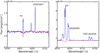 |
Fig. 2. Stellar continuum fitting in the blue and red spectra of NGC 1365, one of the galaxies targeted by the S7 survey. The flux calibrated raw spectrum (blue curve) and the stellar continuum fit to the spectrum using pPXF (red curve) are shown. Left panel: integrated blue spectrum extracted from the entire S7 FOV and zoomed in the region around Hβ and [O III]λ4959,5007 emission lines. Right panel: spectra in the red cube zoomed in the region around [N II]λ6549,6585, Hα, and the [S II] doublet. The x-axis in both the panels shows the observed wavelength. |
The emission line fitting then follows a two-step procedure. First, we perform the line fitting in an integrated spectrum, the results of which is used as a prior for fitting across every pixel in the data cube. The robustness of the line fitting across every spaxel was checked by mapping the residuals of the fit across the wavelengths with [S II] emission. The extraction of the integrated spectrum was done from the entire S7 field of view except the bottom two rows of pixels, due to instrumental defects. This spectrum was then used to derive an average value of electron density integrated over all the pixels. We performed Gaussian line fitting primarily for Hβ, [O III] λ4959,5007, [N II] λ6549,6585, Hα, and the [S II] doublet. We used the IDL fitting routine MPFIT (Markwardt 2012), which fits emission lines based on the minimizing-χ2 method, for simultaneous fitting of the nuclear continuum and the emission lines. The emission lines were reproduced using multiple Gaussian components. Initially a single Gaussian component was fitted and the addition of further Gaussian components depended on whether parameters relevant for this work (e.g. the total flux and width of [S II] doublet) became stable within ≲10%. We classify the individual Gaussian components as narrow or broad based on their width (FWHM). For targets without an active outflow, only narrow Gaussian components with width ≤200 km s−1 were required to fit the [S II] emission lines, while for the targets with an outflow, additional broad Gaussian components with width ≥500 km s−1 were required. The width of the narrow component is consistent with the fact that the narrow emission might originate from the disk and is also similar to the values previously observed in the literature (e.g. Harrison et al. 2014; Brusa et al. 2015).
A few constraints were employed while performing the line fitting to avoid any degeneracy in the multiple component fits. The line widths were constrained to be always greater than 100 km s−1 to avoid any spurious detection due to the presence of skylines. The line widths of each narrow component were coupled to each other assuming that all these components originate from the same region of the host galaxy. In most of our subsample, the Hα profile shows the presence of a relatively faint but a very broad component possibly originating from the BLR. These broad lines from the Hα complex are not extended enough to affect the fluxes of the [S II] doublet (see Thomas et al. 2017). We also coupled the relative emission line flux ratios for the doublets [O III]λ4959,5007 and [N II]λ6549,6585 based on theoretical values (e.g. Storey & Zeippen 2000; Dimitrijević et al. 2007).
With the emission line models for the integrated spectrum in hand, the multiple component line fitting was performed for each pixel across the FOV to create flux and density maps (explained in Sect. 3.2). While performing the pixel-by-pixel line fitting, we allow minor variations with respect to the values obtained in the integrated emission line fitting in the line width and its centroid to account for the shifts due to rotation of the host galaxy. The fluxes were always kept positive as we do not expect or assume the presence of absorption features once the stellar continuum has been subtracted. In the presence of broad lines from the BLR, we subtract this broad component (mainly in the case of Hα) with the same centroid and width as that obtained in the integrated spectrum and only allowed variations in the flux. The consistency of the results obtained using this method was checked by comparison with the maps obtained with the LZIFU fitting procedure (see Ho et al. 2016; Hampton et al. 2017), and the final density maps (Sect. 3.2) do not significantly differ from the two methods.
3.2. Determination of electron densities
To calculate electron densities, we use the prescription employed in Sanders et al. (2016)
 (1)
(1)
where the flux ratio R = f ([S II]λ6716)/f ([S II]λ6731), and a = 0.4315, b = 2107 and c = 627.1. In the case of targets with an outflow, the density maps were created using the ratio of the total flux of the individual emission lines of the [S II] doublet to determine overall density within the ionized medium, as well as the flux ratio of the broad components separately to determine the density in the outflowing medium. A number of assumptions have been made to arrive at Eq. (1) by Sanders et al. (2016), which we briefly summarize here (see also Kaasinen et al. 2017). The electron temperature is assumed to be 10 000 K and the electron densities are directly proportional to the H II region pressure. This may lead to an overestimation of densities in metal-rich galaxies. However, the errors due to these assumptions are significantly smaller than the measurement errors. For the flux ratios close to unity (0.7 < R < 1.45), the density ratio can vary between ∼50 and 2000 cm−3. Such a large variation further reinforces the need for high S/N spectra for the analysis.
The almost linear relation between the [S II] doublet ratio and the electron density makes it effective in measuring the electron density in the above-mentioned ranges. However, the [S II] doublet flux ratio saturates for R > 1.45 and R > 0.7 corresponding to the density values of ∼50 and ∼2000 cm−3, the exact values of the lower and upper limits depend on the data quality4. Therefore, we clip the minimum and maximum values to 50 and 2000 cm−3, respectively. After arriving at the electron density value from the integrated spectrum, we calculate the density across the FOV, as explained in Sect. 3.1, to create electron density maps which are shown in Sect. 4. As mentioned earlier, for targets with an outflow, we create electron density maps from the total flux of the [S II] doublet and from the broad component to determine the density within the outflowing medium. To determine whether the density patterns observed are due to star formation or AGN, we have also created spatially resolved diagnostic diagrams (see Sect. 3.3 for explanation).
The error cubes obtained from the PYWIFES reduction were used to create 1000 mock data cubes by the addition of Gaussian random noise from the corresponding error values. We repeated the line fitting procedure for each of these mock data cubes to obtain a standard deviation of various parameters used in the analysis. We obtain similar error values in the electron density while taking into account error propagation from the flux ratio in Eq. (1).
3.3. Spatially resolved BPT diagrams
The emission line ratios [O III]/Hβ and [N II]/Hα are often used to distinguish the ionization mechanism of a nebular gas using diagnostic diagrams known as the Baldwin, Phillips & Terlevich (BPT) diagrams (Baldwin et al. 1981). The most commonly used demarcations to distinguish between the ionization by star formation and by an AGN, or a combination of the two, is given by the theoretical models of Kewley et al. (2001) and Kauffmann et al. (2003).
We created spatially resolved diagnostic diagrams for each target to understand whether the density morphology observed across the S7 FOV is affected by AGNs or star formation processes (see also Belfiore et al. 2016; Davies et al. 2017). Figure 4c shows an example for NGC 1365 where each data point corresponds to every pixel in the S7 FOV. The solid and the dashed lines are the demarcations by Kewley et al. (2001) and Kauffmann et al. (2003) where the area between the two curves corresponds to the AGN-starburst composite region, and below and above these curves we expect a contribution from star formation and AGN alone, respectively. The data points have been colour-coded based on the [N II]/Hα line ratio, which can distinguish the regions ionized by AGN and star formation in the spatially resolved [N II]/Hα map in Fig. 4d for example. We repeat a similar analysis for the rest of the targets which are collectively shown in Figs. 6–8.
4. Results
In this section, we first describe the results for a single target, NGC 1365, as a motivating example and then we report the collective results of the rest of the targets.
4.1. Integrated spectrum
The integrated spectrum of the stellar continuum subtracted “blue” and “red” cubes zoomed around the emission lines Hβ, [O III]λ4959,5007, Hα, [N II], and [S II] doublet is shown for NGC 1365 as an example in Fig. 3. NGC 1365 is a Seyfert 1 galaxy which has a strong Hα emission line with width (FWHM) of ∼1100 km s−1, as can be seen in the middle panel of Fig. 3. The double-peaked narrow emission lines for Hα, [N II] and [S II] profiles suggest that rotation drives this large line width. The fit to each individual peak has a narrower FWHM of ∼165 km s−1. The [O III] profile, shown in the left panel of Fig. 3, appears symmetric with no clear signatures of the presence of a strong ionized outflow. The [S II] spectra for the rest of the targets are presented in Appendix A.
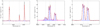 |
Fig. 3. Stellar continuum subtracted integrated spectrum of NGC 1365 showing the Hβ and [O III]λ4959,5007 emission lines (left panel), [N II]λ6548,6585 and Hα (middle panel), and [S II] doublet (right panel). All the wavelengths on the x-axis are the rest frame wavelengths. The underlying black curve shows the observed spectrum and the overlaid red curve shows the overall model. The blue curves show the individual narrow Gaussian components and the magenta curve shows the broad Hα Gaussian component. The vertical dotted lines show the expected position of the Hβ,[O III], [N II], Hα, and [S II] doublet emission lines inferred from the redshift of the targets. |
The electron densities derived using Eq. (1) from the integrated spectrum of NGC 1365 and the rest of the targets are reported in Table 2. The densities mentioned in the table are calculated from the ratio of the total flux of each component of the [S II] doublet. Most of the integrated density values for the targets presented in this paper lie between ∼100 and 330 cm−3 which is comparable to the density values previously reported for the local AGN host galaxies (e.g. Bennert et al. 2006a; Rupke et al. 2017). For the broad outflowing component in NGC 1068, NGC 1266, and NGC 2110, we obtain a density value of 726 ± 90, 1120 ± 295, and 237 ± 78 cm−3, respectively. The [S II] spectrum showing these broad components are shown in Fig. 5. Therefore, from the integrated spectrum analysis, the outflowing component has a significantly higher density compared to the non-outflowing components. This is in line with the density measured with the outflowing components for SDSS targets in Perna et al. (2017) at high redshift (z ∼ 0.7), where the average density was ∼1000 cm−3. However, as explained in the following section, spatially resolved electron density maps show that the high-density scenario is not always true within the outflowing medium.
Observed physical quantities inferred from S7 data.
4.2. Electron density maps
Figure 4 shows the flux maps, resolved diagnostic maps, extinction and density maps, and density profile for NGC 1365 as an example. In all the maps, the black cross in the centre represents the position of the AGN, the red arrow shows north, the magenta contours show the narrow Hα emission, and the orange contours show the [O III] emission at 30%, 50%, and 80% of the peak. The beam at the bottom left of the maps in panels a, b, e, and f shows the PSF (FWHM) during the observations.
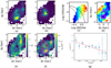 |
Fig. 4. Analysis maps of NGC 1365 shown here as an example. Panels a and b: narrow Hα and [O III]λ5007 flux maps showing the star forming and NLR ionization regions in the host galaxy of NGC 1365, respectively. The red arrow indicates north and the black cross in the centre shows the position of the AGN. Panels c and d: BPT diagram with each point representing the data from every pixel in the S7 FOV, colour-coded on the scale of the [N II]/Hα flux ratio, and the corresponding position of these data points in the image. The spatially resolved BPT map shows the regions ionized by AGN and/or shocks and star formation. The solid and the dotted black line in panel c correspond to the extreme starburst Kewley et al. (2001) line and the Kauffmann et al. (2003) classification, respectively. The magenta contours represent the Hα emission from panel a at levels 30%, 50%, and 80% of the peak, showing that the clumps in the Hα map are indeed sites of star formation. Panel e: extinction map derived from the Hβ/Hα line ratio showing the obscuring regions in NGC 1365. Panel f : electron density map derived from the [S II]λ6716/[S II]λ6731 line ratio (see Sect. 3.2 for further details). The overlaid magenta contours represent the narrow Hα emission from panel a and the orange contours represent the [O III] emission from panel b at levels 30%, 50%, and 80% of the peak. The contour locations show that the electron density is high in sites of star formation. Panel g: electron density profile as a function of radius from the central AGN (black cross on the maps). The blue data points represent the profiles derived from the map itself and red line shows the best fit model assuming an exponential profile (see Sect. 4 for details). The stripped ellipse in the lower left corner of the maps in panels a, b, e and f illustrates the PSF during the observations. |
The narrow Hα emission in NGC 1365 (Fig. 4a) shows a clumpy profile in a ring-like structure around the central AGN. These clumps are consistent with being star forming regions, which is verified by the BPT diagrams in panels c and d in Fig. 4. The [O III] emission in NGC 1365 (Fig. 4b) seems to originate from the central AGN and its morphology and spatial distribution is significantly different from the narrow Hα map.
With the coverage of Hβ and Hα emission lines with WiFeS, we were also able to construct reddening maps (or dust extinction maps) using the Balmer decrement (Hα/Hβ) as shown in Fig. 4e. The extinction map is useful to convert the narrow Hα map to star formation, correcting for any attenuated H II region. We do not expect any significant changes to the electron density maps due to this correction as the [S II] doublet lines are closely spaced leading to similar correction factors in both the fluxes and therefore not a significant change in the flux ratio R in Eq. (1). The extinction maps were obtained assuming a Calzetti et al. (2000) dust attenuation law with RV = 4.05 and a fixed temperature of 10 000 K, which is the same as that derived for the electron density maps. We note that the extinction maps were obtained using only the narrow component of Hα and Hβ, which avoids flux contributions from BLR. For NGC 1365, the extinction map shows high obscuration in the north with respect to the central AGN, where there is also a bright H II clump suggesting that the star formation in this clump might be obscured. The presence of dust in NGC 1365 has also been confirmed by 24 μm Herschel and Spectral and Photometric Imaging Receiver (SPIRE) observations in Alonso-Herrero et al. (2012), where a comparison between the SFR derived from the 24 μm continuum and the narrow Hα line shows that nearly 85% of the ongoing star formation in the central regions of NGC 1365 is taking place in the dust obscured regions. The extinction maps for the rest of the targets are shown in Figs. 6 and 7. Most extinction maps show high extinction at the edges of the H II clumps.
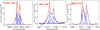 |
Fig. 5. Integrated spectrum around the [S II] doublet of NGC 1068 (left panel), NGC 1266 (middle panel), and NGC 2110 (right panel), the targets showing the presence of an ionized outflow as interpreted from the S7 data. The colour-coding is the same as in Fig. 3. |
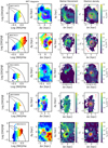 |
Fig. 6. From left to right: data points from each pixel in the S7 FOV on a BPT diagram colour-coded based on the [N II]/Hα flux ratio, corresponding to the spatially resolved BPT map, extinction map, and density map for targets (from top to bottom) NGC 1672, NGC 613, NGC 4691, NGC 6000, and NGC 6221. As in Fig. 4, the magenta and orange contours represent the Hα and [O III] emission at levels 30%, 50%, and 80% of the peak. The red arrow in the density maps indicate north. In all the cases, the narrow Hα contours in magenta almost fall under the star forming region of the BPT diagram showing that there is no strong contribution from the AGN in these areas. All the targets in this figure also show a spatial correlation between sites of high star formation (from the narrow Hα contours) and high density. |
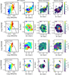 |
Fig. 7. Same as Fig. 6 for targets (top to bottom) NGC 7496, NGC 7469, NGC 5990, and NGC 4303. NGC 7496 and NGC 7469 show the same trend as the targets in Fig. 6, i.e. the sites of high density correspond to sites of high star formation. In the case of NGC 7469, the density pattern extends beyond the narrow Hα emission in the S–E direction and a comparison with the reddening map suggests the possibility of obscured star formation. NGC 5990 and NGC 4303, on the other hand, do not show this spatial correlation (see Sects. 4 and 5 for details). |
Figure 4f shows the density map for NGC 1365 obtained by the pixel-by-pixel analysis of the [S II] doublet with narrow Hα and [O III] contours from the respective maps in panels a and b overlaid in magenta and orange, respectively. From the electron density map of NGC 1365, it is clear that the electron density is high in sites of star forming regions and is spatially uncorrelated with the [O III] emission. This correlation between the star formation and high density is also seen in the maps of the majority of the targets shown in the right panels of Figs. 6 and 7 except NGC 5990 and NGC 4303. In the case of NGC 7469 (second row from top in Fig. 7), in addition to the spatial correlation with the H II regions, the electron density in this target also shows an extension towards the south-east with respect to the central AGN. This site also seems to be a region of high extinction, indicating the possibility of obscured star formation in this region. This suggests that in cases like NGC 7469, density maps could also possibly hint towards sites of obscured star formation in some objects. As mentioned earlier, exceptions to this spatial correlation do exist in targets like NGC 4303 and NGC 5990, as shown in the bottom two panels of Fig. 7; this is discussed in Sect. 5. We can infer the pressure at the centre of galaxies using
![Mathematical equation: $$p/k[{\rm{K c}}{{\rm{m}}^{ - 3}}] ~ 2.4{n_{\rm{e}}}T,$$](/articles/aa/full_html/2018/10/aa32790-18/aa32790-18-eq2.gif) (2)
(2)
where 2.4 is a correction factor for the total number of ions and the temperature T is assumed to be 10 000 K (the same as the assumed temperature for the derivation of electron density for consistency) and ne is the electron density at the centre. The pressures for the sample in this paper are reported in Table 2.
Figure 9 shows the electron density in the outflowing medium derived from the flux ratio of the broad components of the [S II] doublet. The red contours in Fig. 9 represent the broad [O III] emission tracing the outflowing gas in the NLR. For completeness, we also show the density maps derived from the flux ratio of the total flux of the individual lines of the [S II] doublet in Fig. 8, i.e. summing over both narrow and broad Gaussian components, which is often used in literature. A first look at the two sets of maps suggests that the clear spatial correlation between the density and star forming sites (as in the case of non-outflowing targets) ceases to exist for these outflowing targets, partly due to high AGN contamination in the narrow Hα regions inferred from the BPT diagram. Although star formation may also increase the density as the narrow Hα emission is co-spatial with the AGN ionization region, the range of density values is significantly wider than the range observed in the star forming regions in the non-outflowing targets. The density maps from the outflowing component in Fig. 9 suggests that there is no uniform density within the outflowing medium as is often assumed in the mass outflow rate calculations. The density in fact can take a wide range of values, for example from <50 cm−3 to >2000 cm−3 in NGC 1068. These results from spatially resolved maps are in contrast with the high electron density (∼1000 cm−3) reported in outflowing medium from integrated spectrum analysis (e.g. NGC 1068 and NGC 1266 in this paper and the sample in Perna et al. 2017). For targets like NGC 1266, the density at the outflow location traced by [O III] is less than 50 cm−3 throughout, which further reinforces the need for caution when interpreting results obtained from integrated spectrum analysis.
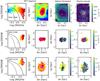 |
Fig. 8. Same as Fig. 6, but for the targets showing AGN-driven outflows: (top to bottom) NGC 1068, NGC 1266, and NGC 2110. The density maps in this figure were obtained from the ratio of the total flux of the individual emission lines of the [S II] doublet, which is often used in literature. |
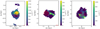 |
Fig. 9. Electron density map in the outflowing broad component in NGC 1068 (left panel), NGC 1266 (middle panel), and NGC 2110 (right panel). The red contours show the location of the outflow as inferred from the broad component of [O III]. The density maps in this figure were obtained from the ratio of the flux of the broad components of the [S II] doublet, which is believed to trace the gas in the outflowing medium. |
The implications of these observations are discussed further in Sect. 5.
4.3. Electron density profiles
The electron density maps presented above are also useful to quantify how the density drops as a function of the distance from the central AGN. To do this, we constructed electron density profiles by extracting integrated density values from circular annuli centred on the AGN and with a width of one pixel, which roughly matches the resolution of the observations. We did not do this exercise for the density measured in the outflowing medium (Fig. 9) as there is no obvious pattern across the three targets. Therefore, we only report the density profile results in the cases where the density maps were obtained from the ratio of the total flux of the individual emission lines of the [S II] doublet. The data points obtained from the electron density map of NGC 1365 are shown as blue circles in panel g of Fig. 4 as an example, while for the rest of the targets the profiles are shown collectively in Fig. 10. The red line in each of the plots shows the model exponential profile as explained below.
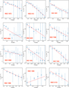 |
Fig. 10. Electron density profiles of the targets presented in this paper. Blue data points show the electron density values obtained from the maps in Figs. 6 and 7, while the solid red line shows the exponential fit to the profile (see text for details). The exponential index is given in Table 2. For the targets with ionized outflows, i.e. NGC 1068, NGC 1266, and NGC 2110 (bottom panels), the density profiles were obtained for the maps presented in Fig. 8. |
From the plots in Fig. 10, it is clear that the electron density decreases as a function of the inclination corrected distance from the centre of the galaxy (except for NGC 1266, see Sect. 5). The drop is density is not necessarily uniform due to the clumps, as in case of NGC 1365 (Fig. 4g). Nevertheless, to a first order, these profiles can generally be fit using an exponential function of the distance from the centre of the galaxy, which can be mathematically expressed as
 (3)
(3)
where α is a normalization constant, β is the exponential index, and R is the distance (in kpc) from the centre, corrected for inclination. The exponential fit for all the targets is shown as a solid red line in Fig. 10. The exponential index for most of these targets lies between 0.1 and 0.2 (see Table 2). Such an exponential function fit gives the least χ2 estimate compared to other models such as an inverse-square drop with distance.
It is apparent from the profiles that in most of the cases the electron density inferred from the ratio of the total flux of the individual emission lines of the [S II] doublet drops to <50 cm−3 for distances larger than 1 kpc from the centre. [O III] emitting regions in targets such as NGC 1365 (Fig. 4) and NGC 613 (Fig. 6) also show low densities (≤50 cm−3). This is valid even in the cases of outflowing targets NGC 1068 and NGC 2110 (Fig. 8), where the density drops to the lower limits for distances larger than 1 kpc from the centre. NGC 1266 is an exception as the presence of outflow seems to increase the density in one direction, and we are limited by the S/N of the [S II] doublet for distances larger than 1 kpc.
The above results of the density profile are not necessarily true for density within the outflowing medium. This is clear from Fig. 9 where the density either increases or decreases from the centre, which is possible due to a turbulent outflowing medium and the presence of shocks.
5. Discussion
One of the main motivations of this study is to constrain the density values in the NLR of AGNs traced by the [O III] emission line and to show how the presence of an ionized outflow affects the density values and its morphology in an attempt to reduce the systematic uncertainties in the estimation of mass outflow rates. Studies often assume a uniform density in the outflowing medium which leads to systematic errors spanning multiple orders of magnitude (e.g. Veilleux et al. 2005; Cano-Díaz et al. 2012; Genzel et al. 2014; McElroy et al. 2015; Husemann et al. 2016; Kakkad et al. 2016; Leung et al. 2017). Although a few studies have calculated electron densities based on the integrated [S II] doublet ratio (e.g. Brusa et al. 2015; Perna et al. 2015b), the analysis in this paper highlights the complexity as well as the differences in interpreting the electron density values when comparing information from the integrated spectrum and a spatially resolved data set.
For the AGNs presented this paper, we find a mean electron density of ∼160 cm−3 calculated from the ratio of the total flux of each component of the [S II] doublet in the spectrum binned over the entire S7 FOV. These binned values are consistent with a recent study by Rupke et al. (2017) who also find the spatially averaged value of electron density to lie between 50 and 410 cm−3 with a median value of 150 cm−3, in a sample of Type 1 radio quiet quasars at z < 0.3. Compared to the integrated electron density values in the local star forming population derived from SDSS, the DR7 sample in Sanders et al. (2016) and Kaasinen et al. (2017), the electron density in the local AGN host galaxies are a factor of ∼5 higher, which might suggest that AGNs are increasing in density or that the high-density gas is associated with triggering the AGNs in the first place. However, we note that the above comparison between the density in local star forming populations and the AGN host galaxies is only suggestive, as the physical scales sampled by the S7 and SDSS spectra are different, and the S7 spectra might be biased to higher density present in the nuclear regions.
The mean electron density in the outflowing medium calculated from the flux ratio of the broad components of the [S II] doublet in the binned spectrum for the targets showing ionized outflows is ∼700 cm−3. The analysis of the integrated spectrum is therefore indicative that the electron density in the outflowing medium is higher by a factor of ∼5 compared to the electron density in the non-outflowing medium. The presence of high electron density in the outflowing medium in AGN host galaxies has also been inferred in Perna et al. (2017) who report enhanced densities of ∼1200 cm−3 in the outflowing gas for a z < 0.8 sample of AGN host galaxies selected from the SDSS survey using stacked spectrum. High-density outflows (>1000 cm−3) have also been predicted indirectly in Chamberlain et al. (2015) for a broad absorption line (BAL) quasar using column density ratios of SIV and SIV*. However, as reported in Sect. 4, spatially resolved maps of electron density in the outflowing medium shows that this scenario of dense ionized outflow is not always true.
Spatially resolved electron density maps for the targets not having an active ionized outflow suggests that the high-density sites for most of the targets correlate with the location of the H II regions (or star forming regions, e.g. Westmoquette et al. 2011, 2013; McLeod et al. 2015). This observation from the local star forming clumps agrees well with recent results of Shimakawa et al. (2015) and Kaasinen et al. (2017) who report an evolution of the overall electron density with star formation rate for star forming galaxies, providing a link between local cloud-scale and global-scale properties within a galaxy. Also, the electron density in the NLR (≲100 cm−3) is much lower than the density in the star forming regions (∼200–600 cm−3). This is very clear in the case of NGC 1365 (Fig. 4). This might be a consequence of the gas density and SFR correlation given by the Kennicutt–Schmidt relation (Kennicutt 1998), while the clumps in the extended NLR traced by the [O III] emission is ionized by the AGN in an ionization cone. In targets such as NGC 5990 and NGC 4303, the correlation between gas density and SFR is absent, which might be due to obscuration from the dust or the host galaxy itself or if the target had previously gone through an outflowing phase from the AGN or starburst (e.g. Riffel et al. 2016).
However, in the presence of an outflow, the correlation between the high-density and star forming sites ceases to exist for the targets presented in this paper. As mentioned earlier, most of the previous studies on spatially resolved electron density maps of AGN host galaxies showing an outflow using the [S II] doublet (e.g. Sharp & Bland-Hawthorn 2010; Westmoquette et al. 2012; Cresci et al. 2015; Rupke et al. 2017; Freitas et al. 2018) use the total flux from each component of the [S II] doublet to calculate the density, as shown for the outflowing sample in this paper in Fig. 8. However, this has the limitation that the contribution from the host galaxy is included, as is the outflowing medium, making it hard to infer the density within the outflow. Figure 9 shows the density derived from the flux ratio of only the broad Gaussian components of the [S II] doublet, which are believed to trace the density of the outflowing medium. In targets with an active outflow inferred from the broad [O III] profiles such as NGC 1068 and NGC 2110, the density can reach values of >1000 cm−3 in certain locations supporting a dense outflow scenario as predicted from the integrated spectrum analysis described earlier. However, this is not true for the entire spatial extent of the outflowing medium, as can be seen from the density maps in Fig. 9. The maps show that the density can be between <50 cm−3 and ∼2000 cm−3 with high-density clumps most likely arising as a result of a turbulent medium which gives rise to shocks and possibly a pressurized medium within the outflow. From the observations presented above, an outflowing medium therefore does not have a uniform density; instead, it shows a wider range in density compared to star forming regions, which is in contrast with the uniform density assumption often used in the literature for mass outflow rate estimations. Therefore, our results suggest that the outflow models should include variable electron density instead of uniform density assumption.
Based on the electron density profiles of all the targets but NGC 1266, we do not expect very high densities for distances larger than 1 kpc from the central AGN. Since the density measurements from the [S II] doublet ratio has the limitation of measuring densities upwards of 50 cm−3, the maps constrain the density values to ≤50 cm−3 in all the galaxies for r ≥ 1 kpc. We note that the S7 field of view only allows us to probe the inner few kpc of the host galaxies. If this trend continues, we might expect much lower densities in the outskirts of the galaxy. Assuming that a trend in the drop in electron density observed within the S7 FOV continues across the entire scale of the galaxy, we would expect the electron density to remain in the lower limit of <50 cm−3 in the outskirts of the galaxy, which can be probed by instruments with a wider FOV, such as MUSE. This, however, might not be true in the case of high-redshift galaxies, as discussed later. The drop in density profile is absent in one outflowing target NGC 1266, which can be attributed to a combination of high nuclear obscuration and the presence of shocks from outflows in multiple phases (e.g. Alatalo et al. 2015; Glenn et al. 2015). Also, we are limited by the S/N ratio of the [S II] to probe the density in the outer regions in NGC 1266. As mentioned earlier in Sect. 4.3, we did not construct such profiles for the outflowing medium as there is no trend, as seen in Fig. 9.
For galaxies at high redshift, the results obtained in this paper might not hold true due to the changing ISM conditions. Observations and theoretical models over the past decade have shed light on the history of star formation and ISM gas and dust content as a function of cosmic time (e.g. Silk & Mamon 2012; Madau & Dickinson 2014; Popping et al. 2017). It is now accepted that the volume averaged star formation rate was at its maximum in the universe at 1 < z < 3 and that the gas content is also higher by an order of magnitude at this epoch (e.g. Scoville et al. 2014). Taking into account the evolution of star formation rate along with our observation that the higher density sites spatially correlate with the H II regions, we would expect the average electron density to also increase as a function of redshift. As mentioned earlier, this has been true in the case of star forming galaxies in recent papers by Shimakawa et al. (2015), Sanders et al. (2016), and Kaasinen et al. (2017), who show an increase in density of a factor of ∼5–10 when compared with the average electron density of the local samples.
Observations have shown that high-redshift galaxies have the potential to host more powerful and extended AGN-driven outflows compared to the local counterparts due to higher mass accretion rates. Therefore, the conditions of the outflowing medium might be significantly different from the galaxies presented in this paper. Current observational capabilities do not provide enough spatial resolution to do a similar study at redshifts higher than ∼1. With upcoming facilities like the James Webb Space Telescope (JWST) and the Narrow Field Mode (NFM) on board MUSE/VLT, it would be possible to probe the ISM conditions within AGN host galaxies to a much wider redshift space.
6. Summary and conclusions
In this paper, we have presented spatially resolved electron density maps of a sample of low-redshift AGN host galaxies derived from the S7 survey using the optical [S II]λ6716,6731 diagnostic lines, which trace the gas in the warm ionized phase. Being a very crucial parameter in the estimation of physical quantities such as the mass outflow rates and energy associated with outflows, we have attempted to understand how the values of electron density and its morphology is affected by the presence of AGN ionization, star formation, or outflows. The following points summarize the main results of this paper:
We find a mean electron density of ∼160 cm−3 calculated using the ratio of the total flux of each component of the [S II] doublet for the low-redshift AGN sample presented in this paper. This value is consistent with recent literature results of electron density calculated from integrated spectra for low-redshift AGNs.
For AGN host galaxies which do not show the presence of an ionized outflow, the electron density maps spatially correlate with narrow Hα maps tracing star formation. For these non-outflowing targets, we find that the electron density in the NLR (≲100 cm−3) is lower than the density in the star forming regions (∼200–600 cm−3). Such small-scale observations agree well with recent results suggesting the evolution of electron density with star formation from integrated spectrum at high redshift.
We find a non-uniform distribution of electron density in the outflowing medium calculated from the flux ratio of the broad component of the [S II] doublet with values ranging from ≲50 cm−3 to ≳2000 cm−3. Our results therefore suggest the need to include variable electron density within the outflowing medium instead of the uniform density assumption. Unlike the non-outflowing targets, the high density does not show a correlation with the star forming sites for the targets presented in this paper.
Radial density profiles of most of the AGN host galaxies suggest a drop in density to <50 cm−3 for distances larger than 1 kpc from the central AGN. The radial density profiles are best fit with an exponential function with a mean exponential index of ∼0.15. On the other hand, the density within the outflowing medium do not show any common pattern, most likely due to the presence of shocks arising out of a turbulent medium.
Due to different ISM conditions at high redshift, i.e. AGNs being more luminous and powerful and extended outflows more common, the results of the current work may not hold true at high redshifts. Therefore, it is essential to have a spatially resolved electron density study for galaxies at high redshift as well, where the effect of radiation pressure on the surrounding ISM seems dominant due to the peak activity of accretion rate of black holes. With upcoming instruments such as the Narrow Field Mode on MUSE and Near-Infrared Spectrograph (NIRSpec) and High Angular Resolution Monolithic Optical and Near-infrared Integral field spectrograph (HARMONI) on board the James Webb Space Telescope (JWST) and the European Extremely Large Telescope (E-ELT), respectively, which will provide unprecedented angular resolution, such a study can be extended to a wider redshift range. While WiFeS is ideal for probing the central few kpc of the host galaxies in nearby AGNs, future studies with MUSE and its wide FOV will be able to probe the outskirts of these low-redshift galaxies as well.
FOcal Reducer/low dispersion Spectrograph.
ESO Multi-Mode Instrument.
The lower and the upper values of 50 cm−3 and 2000 cm−3 are not strict limits and depend on the quality of the data used and can be anywhere from <50–100 cm−3 to 10 000 cm−3.
We have made a more conservative estimate to the upper limit, unlike Sanders et al. (2016) who use a limit that goes beyond a few tens of thousands.
Acknowledgments
The authors thank the anonymous referee for the very constructive comments that improved the paper. B.G. acknowledges the support of the Australian Research Council as the recipient of a Future Fellowship (FT140101202). M.D. acknowledges the support of the Australian Research Council (ARC) through Discovery project DP16010363. Parts of this research were conducted by the Australian Research Council Centre of Excellence for All Sky Astrophysics in 3 Dimensions (ASTRO 3D), through project number CE170100013.
References
- Alatalo, K., Lacy, M., Lanz, L., et al. 2015, ApJ, 798, 31 [NASA ADS] [CrossRef] [Google Scholar]
- Alonso-Herrero, A., Sánchez-Portal, M., Ramos Almeida, C., et al. 2012, MNRAS, 425, 311 [NASA ADS] [CrossRef] [Google Scholar]
- Baldwin, J. A., Phillips, M. M., & Terlevich, R. 1981, PASP, 93, 5 [NASA ADS] [CrossRef] [EDP Sciences] [Google Scholar]
- Belfiore, F., Maiolino, R., Maraston, C., et al. 2016, MNRAS, 461, 3111 [Google Scholar]
- Bennert, N., Jungwiert, B., Komossa, S., Haas, M., & Chini, R. 2006a, A&A, 459, 55 [NASA ADS] [CrossRef] [EDP Sciences] [Google Scholar]
- Bennert, N., Jungwiert, B., Komossa, S., Haas, M., & Chini, R. 2006b, A&A, 456, 953 [NASA ADS] [CrossRef] [EDP Sciences] [Google Scholar]
- Bennert, N., Jungwiert, B., Komossa, S., Haas, M., & Chini, R. 2006c, A&A, 446, 919 [NASA ADS] [CrossRef] [EDP Sciences] [Google Scholar]
- Brusa, M., Bongiorno, A., Cresci, G., et al. 2015, MNRAS, 446, 2394 [NASA ADS] [CrossRef] [Google Scholar]
- Bundy, K., Bershady, M. A., Law, D. R., et al. 2015, ApJ, 798, 7 [NASA ADS] [CrossRef] [Google Scholar]
- Cano-Díaz, M., Maiolino, R., Marconi, A., et al. 2012, A&A, 537, L8 [NASA ADS] [CrossRef] [EDP Sciences] [Google Scholar]
- Cappellari, M., & Emsellem, E. 2004, PASP, 116, 138 [NASA ADS] [CrossRef] [Google Scholar]
- Chamberlain, C., Arav, N., & Benn, C. 2015, MNRAS, 450, 1085 [NASA ADS] [CrossRef] [Google Scholar]
- Childress, M. J., Vogt, F. P. A., Nielsen, J., & Sharp, R. G. 2014, APSS, 349, 617 [NASA ADS] [Google Scholar]
- Comerford, J. M., Barrows, R. S., Müller-Sánchez, F., et al. 2017, ApJ, 849, 102 [NASA ADS] [CrossRef] [Google Scholar]
- Cresci, G., Marconi, A., Zibetti, S., et al. 2015, A&A, 582, A63 [NASA ADS] [CrossRef] [EDP Sciences] [Google Scholar]
- Croom, S. M., Lawrence, J. S., Bland-Hawthorn, J., et al. 2012, MNRAS, 421, 872 [NASA ADS] [Google Scholar]
- Darvish, B., Mobasher, B., Sobral, D., et al. 2015, ApJ, 814, 84 [NASA ADS] [CrossRef] [Google Scholar]
- Davies, R. L., Groves, B., Kewley, L. J., et al. 2017, MNRAS, 470, 4974 [NASA ADS] [CrossRef] [Google Scholar]
- Dimitrijević, M. S., Popović, L. Č., Kovačević, J., Dačić, M., & Ilić, D. 2007, MNRAS, 374, 1181 [NASA ADS] [CrossRef] [Google Scholar]
- Dopita, M. A., Fischera, J., Sutherland, R. S., et al. 2006, ApJ, 647, 244 [NASA ADS] [CrossRef] [Google Scholar]
- Dopita, M. A., Shastri, P., Davies, R., et al. 2015, ApJS, 217, 12 [NASA ADS] [CrossRef] [Google Scholar]
- Freitas, I. C., Riffel, R. A., Storchi-Bergmann, T., et al. 2018, MNRAS, 476, 2760 [NASA ADS] [CrossRef] [Google Scholar]
- Genzel, R., Förster Schreiber, N. M., Rosario, D., et al. 2014, ApJ, 796, 7 [Google Scholar]
- Glenn, J., Rangwala, N., Maloney, P. R., & Kamenetzky, J. R. 2015, ApJ, 800, 105 [NASA ADS] [CrossRef] [Google Scholar]
- Greene, J. E., Zakamska, N. L., & Smith, P. S. 2012, ApJ, 746, 86 [NASA ADS] [CrossRef] [Google Scholar]
- Hainline, K. N., Shapley, A. E., Kornei, K. A., et al. 2009, ApJ, 701, 52 [NASA ADS] [CrossRef] [Google Scholar]
- Hampton, E. J., Medling, A. M., Groves, B., et al. 2017, MNRAS, 470, 3395 [NASA ADS] [CrossRef] [Google Scholar]
- Harrison, C. M., Alexander, D. M., Mullaney, J. R., & Swinbank, A. M. 2014, MNRAS, 441, 3306 [Google Scholar]
- Harrison, C. M., Alexander, D. M., Mullaney, J. R., et al. 2016, MNRAS, 456, 1195 [NASA ADS] [CrossRef] [Google Scholar]
- Heckman, T. M., Armus, L., & Miley, G. K. 1990, ApJS, 74, 833 [NASA ADS] [CrossRef] [Google Scholar]
- Ho, I.-T., Medling, A. M., Groves, B., et al. 2016, Ap&SS, 361, 280 [CrossRef] [Google Scholar]
- Husemann, B., Scharwächter, J., Bennert, V. N., et al. 2016, A&A, 594, A44 [NASA ADS] [CrossRef] [EDP Sciences] [Google Scholar]
- Kaasinen, M., Bian, F., Groves, B., Kewley, L. J., & Gupta, A. 2017, MNRAS, 465, 3220 [NASA ADS] [CrossRef] [Google Scholar]
- Kakkad, D., Mainieri, V., Padovani, P., et al. 2016, A&A, 592, A148 [Google Scholar]
- Kauffmann, G., Heckman, T. M., Tremonti, C., et al. 2003, MNRAS, 346, 1055 [Google Scholar]
- Kennicutt, Jr., R. C. 1998, ARA&A, 36, 189 [Google Scholar]
- Kewley, L. J., Dopita, M. A., Sutherland, R. S., Heisler, C. A., & Trevena, J. 2001, ApJ, 556, 121 [Google Scholar]
- Kewley, L. J., & Dopita, M. A. 2002, ApJS, 142, 35 [NASA ADS] [CrossRef] [Google Scholar]
- Kewley, L. J., Dopita, M. A., Leitherer, C., et al. 2013, ApJ, 774, 100 [NASA ADS] [CrossRef] [Google Scholar]
- Leung, G. C. K., Coil, A. L., Azadi, M., et al. 2017, ApJ, 849, 48 [NASA ADS] [CrossRef] [Google Scholar]
- Liu, G., Zakamska, N. L., Greene, J. E., Nesvadba, N. P. H., & Liu, X. 2013, MNRAS, 436, 2576 [NASA ADS] [CrossRef] [Google Scholar]
- Madau, P., & Dickinson, M. 2014, ARA&A, 52, 415 [NASA ADS] [CrossRef] [Google Scholar]
- Markwardt, C. 2012, Astrophysics Source Code Library [record ascl: 1208.019] [Google Scholar]
- McElroy, R., Croom, S. M., Pracy, M., et al. 2015, MNRAS, 446, 2186 [NASA ADS] [CrossRef] [Google Scholar]
- McLeod, A. F., Dale, J. E., Ginsburg, A., et al. 2015, MNRAS, 450, 1057 [NASA ADS] [CrossRef] [Google Scholar]
- Müller-Sánchez, F., Prieto, M. A., Hicks, E. K. S., et al. 2011, ApJ, 739, 69 [NASA ADS] [CrossRef] [Google Scholar]
- Nesvadba, N. P. H., Lehnert, M. D., Eisenhauer, F., et al. 2006, ApJ, 650, 693 [NASA ADS] [CrossRef] [Google Scholar]
- Osterbrock, D. E., & Ferland, G. J. 2006, Astrophysics of Gaseous Nebulae and Active Galactic Nuclei (Sausalito: University Science Books) [Google Scholar]
- Perna, M., Brusa, M., Cresci, G., et al. 2015a, A&A, 574, A82 [NASA ADS] [CrossRef] [EDP Sciences] [Google Scholar]
- Perna, M., Brusa, M., Salvato, M., et al. 2015b, A&A, 583, A72 [NASA ADS] [CrossRef] [EDP Sciences] [Google Scholar]
- Perna, M., Lanzuisi, G., Brusa, M., Cresci, G., & Mignoli, M. 2017, A&A, 606, A96 [Google Scholar]
- Popping, G., Somerville, R. S., & Galametz, M. 2017, MNRAS, 471, 3152 [NASA ADS] [CrossRef] [Google Scholar]
- Riffel, R. A., Colina, L., Storchi-Bergmann, T., et al. 2016, MNRAS, 461, 4192 [NASA ADS] [CrossRef] [Google Scholar]
- Rupke, D. S. N., Gültekin, K., & Veilleux, S. 2017, ApJ, 850, 40 [Google Scholar]
- Sanders, R. L., Shapley, A. E., Kriek, M., et al. 2016, ApJ, 816, 23 [Google Scholar]
- Scoville, N., Aussel, H., Sheth, K., et al. 2014, ApJ, 783, 84 [NASA ADS] [CrossRef] [Google Scholar]
- Sharp, R. G., & Bland-Hawthorn, J. 2010, ApJ, 711, 818 [NASA ADS] [CrossRef] [Google Scholar]
- Shimakawa, R., Kodama, T., Steidel, C. C., et al. 2015, MNRAS, 451, 1284 [NASA ADS] [CrossRef] [Google Scholar]
- Shirazi, M., Brinchmann, J., & Rahmati, A. 2014, ApJ, 787, 120 [NASA ADS] [CrossRef] [Google Scholar]
- Silk, J., & Mamon, G. A. 2012, Res. Astron. Astrophys., 12, 917 [NASA ADS] [CrossRef] [Google Scholar]
- Spence, R. A. W., Tadhunter, C. N., Rose, M., & Rodríguez Zaurín, J. 2018, MNRAS, 478, 2438 [NASA ADS] [CrossRef] [Google Scholar]
- Storchi-Bergmann, T., McGregor, P. J., Riffel, R. A., et al. 2009, MNRAS, 394, 1148 [NASA ADS] [CrossRef] [Google Scholar]
- Storey, P. J., & Zeippen, C. J. 2000, MNRAS, 312, 813 [Google Scholar]
- Sun, A.-L., Greene, J. E., & Zakamska, N. L. 2017, ApJ, 835, 222 [NASA ADS] [CrossRef] [Google Scholar]
- Thomas, A. D., Dopita, M. A., Shastri, P., et al. 2017, ApJS, 232, 11 [NASA ADS] [CrossRef] [Google Scholar]
- Toba, Y., Bae, H.-J., Nagao, T., et al. 2017, ApJ, 850, 140 [NASA ADS] [CrossRef] [Google Scholar]
- Turner, O. J., Cirasuolo, M., Harrison, C. M., et al. 2017, MNRAS, 471, 1280 [NASA ADS] [CrossRef] [Google Scholar]
- Veilleux, S., Cecil, G., & Bland-Hawthorn, J. 2005, ARA&A, 43, 769 [Google Scholar]
- Villar-Martín, M., Arribas, S., Emonts, B., et al. 2016, MNRAS, 460, 130 [NASA ADS] [CrossRef] [Google Scholar]
- Wake, D. A., Bundy, K., Diamond-Stanic, A. M., et al. 2017, AJ, 154, 86 [NASA ADS] [CrossRef] [Google Scholar]
- Westmoquette, M. S., Smith, L. J., & Gallagher, III, J. S. 2011, MNRAS, 414, 3719 [NASA ADS] [CrossRef] [Google Scholar]
- Westmoquette, M. S., Clements, D. L., Bendo, G. J., & Khan, S. A. 2012, MNRAS, 424, 416 [NASA ADS] [CrossRef] [Google Scholar]
- Westmoquette, M. S., Dale, J. E., Ercolano, B., & Smith, L. J. 2013, MNRAS, 435, 30 [NASA ADS] [CrossRef] [Google Scholar]
- Wisnioski, E., Förster Schreiber, N. M., Wuyts, S., et al. 2015, ApJ, 799, 209 [NASA ADS] [CrossRef] [Google Scholar]
- Xu, D., Komossa, S., Zhou, H., Wang, T., & Wei, J. 2007, ApJ, 670, 60 [NASA ADS] [CrossRef] [Google Scholar]
- Zakamska, N. L., Hamann, F., Pâris, I., et al. 2016, MNRAS, 459, 3144 [NASA ADS] [CrossRef] [Google Scholar]
Appendix A: S7 spectra
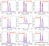 |
Fig. A.1. Spectra showing the [S II] doublet and the line fitting for the targets presented in this paper. |
All Tables
All Figures
|
Fig. 1. Representation of the field of view (FOV) covered by WiFeS instrument used in the S7 survey. The figure shows a 7 × 7 arcmin2 FORS1/VLT image of NGC 1365, one of the galaxies targeted with the S7 survey, as an example. The WiFeS FOV (38 × 25 arcsec2) is overlaid in red. The S7 FOV for the rest of the targets are presented in Dopita et al. (2015) and Thomas et al. (2017). North is up and east is to left. Image credit: ESO. |
| In the text | |
|
Fig. 2. Stellar continuum fitting in the blue and red spectra of NGC 1365, one of the galaxies targeted by the S7 survey. The flux calibrated raw spectrum (blue curve) and the stellar continuum fit to the spectrum using pPXF (red curve) are shown. Left panel: integrated blue spectrum extracted from the entire S7 FOV and zoomed in the region around Hβ and [O III]λ4959,5007 emission lines. Right panel: spectra in the red cube zoomed in the region around [N II]λ6549,6585, Hα, and the [S II] doublet. The x-axis in both the panels shows the observed wavelength. |
| In the text | |
|
Fig. 3. Stellar continuum subtracted integrated spectrum of NGC 1365 showing the Hβ and [O III]λ4959,5007 emission lines (left panel), [N II]λ6548,6585 and Hα (middle panel), and [S II] doublet (right panel). All the wavelengths on the x-axis are the rest frame wavelengths. The underlying black curve shows the observed spectrum and the overlaid red curve shows the overall model. The blue curves show the individual narrow Gaussian components and the magenta curve shows the broad Hα Gaussian component. The vertical dotted lines show the expected position of the Hβ,[O III], [N II], Hα, and [S II] doublet emission lines inferred from the redshift of the targets. |
| In the text | |
|
Fig. 4. Analysis maps of NGC 1365 shown here as an example. Panels a and b: narrow Hα and [O III]λ5007 flux maps showing the star forming and NLR ionization regions in the host galaxy of NGC 1365, respectively. The red arrow indicates north and the black cross in the centre shows the position of the AGN. Panels c and d: BPT diagram with each point representing the data from every pixel in the S7 FOV, colour-coded on the scale of the [N II]/Hα flux ratio, and the corresponding position of these data points in the image. The spatially resolved BPT map shows the regions ionized by AGN and/or shocks and star formation. The solid and the dotted black line in panel c correspond to the extreme starburst Kewley et al. (2001) line and the Kauffmann et al. (2003) classification, respectively. The magenta contours represent the Hα emission from panel a at levels 30%, 50%, and 80% of the peak, showing that the clumps in the Hα map are indeed sites of star formation. Panel e: extinction map derived from the Hβ/Hα line ratio showing the obscuring regions in NGC 1365. Panel f : electron density map derived from the [S II]λ6716/[S II]λ6731 line ratio (see Sect. 3.2 for further details). The overlaid magenta contours represent the narrow Hα emission from panel a and the orange contours represent the [O III] emission from panel b at levels 30%, 50%, and 80% of the peak. The contour locations show that the electron density is high in sites of star formation. Panel g: electron density profile as a function of radius from the central AGN (black cross on the maps). The blue data points represent the profiles derived from the map itself and red line shows the best fit model assuming an exponential profile (see Sect. 4 for details). The stripped ellipse in the lower left corner of the maps in panels a, b, e and f illustrates the PSF during the observations. |
| In the text | |
|
Fig. 5. Integrated spectrum around the [S II] doublet of NGC 1068 (left panel), NGC 1266 (middle panel), and NGC 2110 (right panel), the targets showing the presence of an ionized outflow as interpreted from the S7 data. The colour-coding is the same as in Fig. 3. |
| In the text | |
|
Fig. 6. From left to right: data points from each pixel in the S7 FOV on a BPT diagram colour-coded based on the [N II]/Hα flux ratio, corresponding to the spatially resolved BPT map, extinction map, and density map for targets (from top to bottom) NGC 1672, NGC 613, NGC 4691, NGC 6000, and NGC 6221. As in Fig. 4, the magenta and orange contours represent the Hα and [O III] emission at levels 30%, 50%, and 80% of the peak. The red arrow in the density maps indicate north. In all the cases, the narrow Hα contours in magenta almost fall under the star forming region of the BPT diagram showing that there is no strong contribution from the AGN in these areas. All the targets in this figure also show a spatial correlation between sites of high star formation (from the narrow Hα contours) and high density. |
| In the text | |
|
Fig. 7. Same as Fig. 6 for targets (top to bottom) NGC 7496, NGC 7469, NGC 5990, and NGC 4303. NGC 7496 and NGC 7469 show the same trend as the targets in Fig. 6, i.e. the sites of high density correspond to sites of high star formation. In the case of NGC 7469, the density pattern extends beyond the narrow Hα emission in the S–E direction and a comparison with the reddening map suggests the possibility of obscured star formation. NGC 5990 and NGC 4303, on the other hand, do not show this spatial correlation (see Sects. 4 and 5 for details). |
| In the text | |
|
Fig. 8. Same as Fig. 6, but for the targets showing AGN-driven outflows: (top to bottom) NGC 1068, NGC 1266, and NGC 2110. The density maps in this figure were obtained from the ratio of the total flux of the individual emission lines of the [S II] doublet, which is often used in literature. |
| In the text | |
|
Fig. 9. Electron density map in the outflowing broad component in NGC 1068 (left panel), NGC 1266 (middle panel), and NGC 2110 (right panel). The red contours show the location of the outflow as inferred from the broad component of [O III]. The density maps in this figure were obtained from the ratio of the flux of the broad components of the [S II] doublet, which is believed to trace the gas in the outflowing medium. |
| In the text | |
|
Fig. 10. Electron density profiles of the targets presented in this paper. Blue data points show the electron density values obtained from the maps in Figs. 6 and 7, while the solid red line shows the exponential fit to the profile (see text for details). The exponential index is given in Table 2. For the targets with ionized outflows, i.e. NGC 1068, NGC 1266, and NGC 2110 (bottom panels), the density profiles were obtained for the maps presented in Fig. 8. |
| In the text | |
|
Fig. A.1. Spectra showing the [S II] doublet and the line fitting for the targets presented in this paper. |
| In the text | |
Current usage metrics show cumulative count of Article Views (full-text article views including HTML views, PDF and ePub downloads, according to the available data) and Abstracts Views on Vision4Press platform.
Data correspond to usage on the plateform after 2015. The current usage metrics is available 48-96 hours after online publication and is updated daily on week days.
Initial download of the metrics may take a while.