| Issue |
A&A
Volume 618, October 2018
|
|
|---|---|---|
| Article Number | A74 | |
| Number of page(s) | 15 | |
| Section | Extragalactic astronomy | |
| DOI | https://doi.org/10.1051/0004-6361/201732496 | |
| Published online | 16 October 2018 | |
X-ray study of the double radio relic Abell 3376 with Suzaku
1
SRON Netherlands Institute for Space Research, Sorbonnelaan 2, 3584 CA Utrecht, The Netherlands
e-mail: This email address is being protected from spambots. You need JavaScript enabled to view it.
2
Leiden Observatory, Leiden University, PO Box 9513, 2300 RA Leiden, The Netherlands
3
MTA-Eötvös University Lendület Hot Universe Research Group, Pázmány Péter sétány 1/A, Budapest, 1117 Hungary
4
Institute of Physics, Eötvös University, Pázmány Péter sétány 1/A, Budapest, 1117 Hungary
5
Department of Physics, Tokyo Metropolitan University, 1-1 Minami-Osawa, Hachioji, Tokyo, 192-0397
Japan
6
Department of Earth and Planetary Science, The University of Tokyo, Tokyo, 113-0033 Japan
7
Research Center for the Early Universe, School of Science, The University of Tokyo, Tokyo, 113-0033 Japan
Received:
19
December
2017
Accepted:
20
June
2018
Abstract
We present an X-ray spectral analysis of the nearby double radio relic merging cluster Abell 3376 (z = 0.046), observed with the Suzaku XIS instrument. These deep (∼360 ks) observations cover the entire double relic region in the outskirts of the cluster. These diffuse radio structures are amongst the largest and arc-shaped relics observed in combination with large-scale X-ray shocks in a merging cluster. We confirm the presence of a stronger shock (ℳW = 2.8 ± 0.4) in the western direction at r ∼ 26′, derived from a temperature and surface brightness discontinuity across the radio relic. In the east, we detect a weaker shock (ℳE = 1.5 ± 0.1) at r ∼ 8′, possibly associated with the “notch” of the eastern relic, and a cold front at r ∼ 3′. Based on the shock speed calculated from the Mach numbers, we estimate that the dynamical age of the shock front is ∼0.6 Gyr after core passage, indicating that Abell 3376 is still an evolving merging cluster and that the merger is taking place close to the plane of the sky. These results are consistent with simulations and optical and weak lensing studies from the literature.
Key words: X-rays: galaxies: clusters / shock waves
© ESO 2018
1. Introduction
Galaxy clusters form hierarchically by the accretion and merging of the surrounding galaxy groups and subclusters. During these energetic processes, the intracluster medium (ICM) becomes turbulent and produces cold fronts, the interface between the infalling cool dense gas core of the subcluster and the hot cluster atmosphere, and shock waves, which propagate into the intracluster medium of the subclusters (Markevitch & Vikhlinin 2007). Part of the kinetic energy involved in the merger is converted into thermal energy by driving these large-scale shocks and turbulence, and the other part is transformed into nonthermal energy. Shocks are thought to (re)accelerate electrons from the thermal distribution up to relativistic energies by the first-order Fermi diffusive shock acceleration mechanism (hereafter DSA, Bell 1987; Blandford & Eichler 1987). The accelerated electrons, in the presence of a magnetic field, may produce radio relics via synchrotron radio emission (Ferrari et al. 2008, 2012; Brunetti & Jones 2014). They are generally Mpc-scale sized, elongated and steep-spectrum radio structures (Brüggen et al. 2012; Brunetti & Jones 2014), which appear to be associated with the shock fronts at the outskirts of merging clusters (Finoguenov et al. 2010; Ogrean & Brüggen 2013).
Discoveries of shocks coinciding with radio relics are increasing (Markevitch et al. 2005; Finoguenov et al. 2010; Macario et al. 2011; Ogrean & Brüggen 2013; Bourdin et al. 2013; Eckert et al. 2016b; Sarazin et al. 2016; Akamatsu & Kawahara 2013; Akamatsu et al. 2015, 2017). However, not all merging clusters present the same spatial distribution of the X-ray and radio components (Ogrean et al. 2014; Shimwell et al. 2016). The study of the radial distribution of these thermal and nonthermal components allows us to estimate the dynamical stage of the cluster as well as to understand how the shock propagates and heats the ICM. It can also determine the physical association between radio relics and shocks. The lack of connection between radio relics and shocks in several merging clusters, together with the low efficiency of DSA for ℳ ∼ 2–3 of these shocks, seems to suggest that in some cases the DSA assumption is not enough for the electron acceleration from the thermal pool (Vink & Yamazaki 2014; Vazza & Brüggen 2014; Skillman et al. 2013; Pinzke et al. 2013). For this reason, alternative mechanisms have recently been proposed, such as for example, the re-acceleration of pre-existing cosmic ray electrons (Markevitch et al. 2005; Kang et al. 2012; Fujita et al. 2015, 2016; Kang 2017) and shock drift acceleration (Guo et al. 2014a,b, 2017). However, it is not clear what type of mechanism is involved and whether all relics need additional mechanisms or not. Some merging clusters present different results, as for example “El Gordo” (Botteon et al. 2016b) is consistent with the DSA mechanism. However, A3667 South (Storm et al. 2018), CIZA J2242.8+5301 (Hoang et al. 2017) and A3411-3412 (van Weeren et al. 2017) challenge the direct shock acceleration of electrons from the thermal pool. Therefore, it is not possible to provide a definitive explanation for these discrepancies.
In this paper, we analyze the spatial distribution of thermal and nonthermal components in Abell 3376, (hereafter A3376), based on Suzaku observations (Mitsuda et al. 2007). We have also used XMM-Newton and Chandra observations to support and confirm the results obtained with Suzaku. A3376 is a nearby (z = 0.046, Struble & Rood 1999), bright and moderately massive (M200 ∼ 4–5 × 10¹⁴M⊙, Durret et al. 2013; Monteiro-Oliveira et al. 2017) merging galaxy cluster. This merging system has two giant (∼Mpc) arc-shaped radio relics in the cluster outskirts, discovered by Bagchi et al. (2006). The radio observations (Bagchi et al. 2006; Kale et al. 2012; George et al. 2015), see Fig. 1, reveal complex radio structures at the western and eastern directions. In the west, A3376 shows a lowly polarized wide (∼300 kpc) relic with a non-aligned magnetic field (Kale et al. 2012). In the east, the relic is divided in three parts: the northern faint relic with steep spectral index; an elongated and polarized bright relic; and an additional “notch” with a ∼500 kpc extension toward the center (α ∼ –1.5) (Kale et al. 2012; Paul et al. 2011). Radio spectral index studies, assuming diffusive shock acceleration, with an estimated ℳ∼ 2–3, which is consistent with the previous X-ray study by Akamatsu et al. (2012) of the western relic. A3376 includes two brightest cluster galaxies (BCG), coincident with two overdensities in projected galaxy distribution. BCG1 (ESO 307-13, RA = 6h00m41s.10, Dec = −40°02′40″.00) belongs to the west subcluster, while BCG2 (2MASX J06020973-3956597, RA = 6h02m09s.70, Dec = −39°57′05″.00) is located close to the X-ray peak emission at the east subcluster. The N-body hydrodynamical simulations of Machado & Lima Neto (2013) reproduce a bimodal merger system, with a mass ratio of 3–6:1, formed by one compact and dense subcluster, which crossed at high velocity and disrupted the core of the second massive subcluster ∼0.5–0.6 Gyr ago. This merger scenario was later corroborated by the optical analysis of Durret et al. (2013) and the weak lensing study of Monteiro-Oliveira et al. 2017.
For this study, we used the values of protosolar abundances (Z⊙) reported by Lodders et al. (2009). The abundance of all metals are coupled to Fe. We used a Galactic absorption column of NH, total = 5.6 × 1020 cm−2 (Willingale et al. 2013) for all the fits. We assumed cosmological parameters H0 = 70 km s−1 Mpc−1, ΩM = 0.27 and ΩΛ = 0.73, respectively, which give 54 kpc per 1 arcmin at z = 0.046. The virial radius is adopted as r200, the radius where the mean interior density is 200 times the critical density at the redshift of the source. For our cosmology and redshift we used the approximation of Henry et al. (2009): (1)
(1)
where E(z) = (ΩM(1 + z)3 + 1 − ΩM)1/2, r200 is 1.76 Mpc (∼32.6′) with ⟨kT⟩ = 4.2 keV as calculated by Reiprich et al. (2013). All errors are given at 1σ (68%) confidence level unless otherwise stated and all the spectral analysis made use of the modified Cash statistics (Cash 1979); Kaastra 2017.
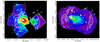 |
Fig. 1. Left: Suzaku smoothed image in the 0.5–10 keV band of A3376 (pixel = 8″ and Gausssian 2-D smooth σ = 16″). The white boxes represent the Suzaku XIS FOVs for the C, W1, W2, N, E and S observations listed in Table 1. BCG1 is shown as a black cross and BCG2 as a blue cross. Right: XMM-Newton image in the 0.5–10 keV band of A3376. The white contours correspond to VLA radio observations kindly provided by Dr. R. Kale. |
Observations and exposure times.
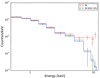 |
Fig. 2. Correction of the XIS1 excess in the outer region of the E observation of A3376. The best-fit ICM spectrum is shown as a blue line. The Suzaku XIS BI spectra are shown without (red) and with (green) a 13% increase in the NXB level, respectively. |
2. Observations and data reduction
Table 1 and Fig. 1 summarize the observations used for the present analysis. As shown in Fig. 1 six different Suzaku pointings have been used together with two additional XMM-Newton observations. Three of the Suzaku pointings are located in the central and western region (hereafter named as C, W1 and W2), which were obtained in 2005 and 2006, respectively. The other three observations (2013) cover the north (N), east (E), and south (S) of the outer eastern region. The combined observations cover the complete relic structures of A3376 as the western relic (W1 and W2), center (C) and eastern relic (N, E, and S). The total effective exposure time of the Suzaku data after screening and filtering of the cosmic-ray cut-off rigidity (COR2, Tawa et al. 2008) is ∼360 ks.
All observations have been performed with the normal 3 × 3 or 5 × 5 clocking mode of the X-ray imaging spectrometer (hereafter XIS, Koyama et al. 2007). This instrument had four active detectors: XIS0, XIS2 and XIS3 (front-side illuminated, FI) and XIS1 (back-side illuminated, BI). On November 9, 2006 the XIS2 detector suffered a micrometeorite strike1 and was no longer operative. The XIS0 detector had a similar accident in 2010 and a part of the segment A was damaged2. In the same year the amount of charge injection for XIS1 was increased from 2 to 6 keV, which leads to an increase in the non-X-ray background (NXB) level of XIS1. For that reason an additional screening has been applied to minimize the NXB level following the process described in the Suzaku Data Reduction Guide3.
We used HEAsoft version 6.20 and CALDB 2016-01-28 for all Suzaku analysis presented here. We have applied standard data screening with the elevation angle > 10° above the Earth and cut-off rigidity (COR2) > 8 GV to increase the signal to noise. The energy range of 1.7–1.9 keV was ignored in the spectral fitting owing to the residual uncertainties present in the Si-K edge.
For the point sources identification and exclusion, we used XMM-Newton observations (ID: 0151900101 and 0504140101, see Table 1). We applied the data reduction software SAS v14.0.0 for the XMM-Newton EPIC instrument with the task named edetect_chain. We used visual inspection for the point sources identification beyond the XMM-Newton observations in the east. We derived the surface brightness (SB) profiles from the XMM-Newton and Chandra (ID: 3202, see Table 1) observations. We used CIAO 4.8 with CALDB 4.7.6 for the data reduction of Chandra observations. Moreover, the Suzaku offset observation of Q0551-3637, located at ∼4 ° distance from A3376, was analyzed to estimate the sky background components as described in the following section.
3. Spectral analysis and results
3.1. Spectral analysis approach
In our spectral analysis of A3376, we have assumed that the observed spectra include the following components: optically thin thermal plasma emission from the ICM, the cosmic X-ray background (CXB), the local hot bubble (LHB), the Milky Way halo (MWH) and non X-ray background (NXB). We first generated the non X-ray background spectra using xisnxbgen (Tawa et al. 2008). Secondly, we identified the point sources present in our data using the two observations of XMM-Newton (see Table 1) and extracted them with a radius of 1–3′ from the Suzaku observations. We have estimated the sky background emission consisting of CXB, LHB, and MWH from the Q0551-3637 observation at 3.8° from A3376 (see Sect. 3.2). We assumed that the sky background component is uniformly distributed along the A3376 extension. We generated the redistribution matrix file (RMF) using xisrmfgen and the ancillary response file (ARF) with xisimarfgen (Ishisaki et al. 2007) considering a uniform input image (r = 20′).
A proper estimation of the background components is crucial, specially in the outskirts of galaxy clusters, where usually the X-ray emission of the ICM is low and the spectrum can be background dominated. The X-ray shock fronts and radio relics are usually located at these outer regions.
We performed a temperature deprojection assuming spherical symmetry to check the projection effect on the temperature profiles. We applied the method described in Blanton et al. (2003) for the post-shock regions, which are affected by projection of the emission of the outer and cooler regions. The results of the deprojection fits are consistent within 1σ uncertainties with the projected temperatures. For this reason, we used the projected fits in this work.
In our spectral analysis, we used SPEX4 (Kaastra et al. 1996) version 3.03.00 with SPEXACT version 2.07.00. We carried out the spectral fitting in different annular regions as detailed in the sections below. The spectra of the XIS FI and BI detectors were fitted simultaneously and binned using the method of optimal binning (Kaastra & Bleeker 2016). For all the spectral fits, the NXB component is subtracted using the trafo tool in SPEX. The free parameters considered in this study are the temperature kT, the normalization Norm and the metal abundance Z for the inner regions r ≤ 9′ of the ICM component. For the outer regions (r > 10′) we fixed the abundance to 0.3 Z⊙ as explained by Fujita et al. (2008) and Urban et al. (2017).
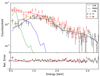 |
Fig. 3. Q0551-3637 spectrum used for the sky background estimation. The Suzaku XIS FI, BI, the LHB, MWH and CXB components are shown in black, red, green, blue, and orange, respectively. The LHB, MWH, and CXB have been represented relative to the BI spectrum. |
Background components derived from the Q0551-3637 observation.
3.2. Estimation of the background spectra
The NXB component was obtained as the weighted sum of the XIS Night Earth observations and it was compiled for the same detector area and COR2 condition (COR2 > 8 GV) during 150 days before and after the observation date. In this way the long-term variation of the XIS detector background due to radiation damage can be constrained. The systematic errors corresponding to the NXB intensity are considered to be ± 3% (Tawa et al. 2008). For the most recent observations (E, N, and S), where a new spectral analysis approach was proposed for XIS15 because of the charge injection increase to 6 keV, we detected an excess of source counts in the high energy band (> 10 keV). We managed to compensate for this excess by increasing the NXB level by 13%. In this way the source level (ICM) follows the spectral shape of the CXB at high energies (see Fig. 2).
As mentioned in Sect. 2, the point source identification in the Suzaku FOV was realized using two XMM-Newton observations. The SAS task named edetect_chain was applied in four different bands (0.3–2.0 keV, 2.0–4.5 keV, 4.5–7.5 keV, and 7.5–12 keV) using EPIC pn and MOS data. We used a simulated maximum likelihood value of ten. After this, we combined the detections in these four bands and estimated the flux of each source in a circle with a radius of 0.6′. We established the minimum of flux detection of the extracted sources as Sc = 10−17 W m−2 in the energy band 2–10 keV. Although this limit is lower than the level reported by Kushino et al. (2002)Sc = 2 × 10⁻¹⁶ W m−2, we obtained an acceptable logN-logS distribution contained within the Kushino et al. (2002) limits (see their Fig. 20). We excluded in the Suzaku observations the identified point sources with a radius of 1 arcmin in order to account for the point spread function (PSF) of XIS (Serlemitsos et al. 2007). As a result, our CXB intensity after the point sources extraction for the 2–10 keV band was estimated as 5.98 × 10⁻¹¹ W m−2 sr−1. This value is within ± 10% agreement with Cappelluti et al. (2017), Akamatsu et al. (2012) and Kushino et al. (2002).
As a sanity check, we compared the sky background level of ROSAT observations for the outermost region of A3376 (r = 30′ − 60′) and the offset pointing Q0551-3637 (r = 3′ − 20′) using the HEASARC X-ray Background Tool6 in the band R45 (0.4–1.2 keV). This band contains most of the emission of the sky background. The R45 intensities in the units of 10−6 counts s−1 arcmin−2 are 125.3 ± 5.0 for the A3376 outer ring and 114.4 ± 18.5 for Q0551-3637. Both values are in good agreement.
We used the same Sc = 10−17 W m−2 for extracting the point sources in the offset Suzaku observation of Q0551-3637. We also excluded a circle of 3′ centered around the quasar with the same name, which is the brightest source of this region. Thereafter, we fitted the resultant spectra using NH = 3.2 × 1020 cm−2 (Willingale et al. 2013), considering the emission of three sky background components at redshift zero and metal abundance of one. For the FI and BI detectors we used the energy ranges of 0.5–7.0 keV and 0.5–5.0 keV, respectively. The two Galactic components are modeled with: LHB (fixed kT = 0.08 keV), unabsorbed cie model (collisional ionization equilibrium in SPEX) and MWH (fixed kT = 0.27 keV), absorbed cie. The third component is the CXB modeled as an absorbed powerlaw with fixed Γ = 1.41. The complete sky background model is: (2)
(2)
Best-fit parameters are listed in Table 2, and the sky background components are shown in Fig. 3. For the calculation of the systematic uncertainties of the CXB fluctuation due to unresolved point sources (σ/ICXB) we have used Eq. (3) proposed by Hoshino et al. (2010) in each spatial region of Fig. 4 and Fig. 7 as (3)
(3)
where (σGinga/ICXB) = 5, Ωe, Ginga = 1.2 deg2, Sc, Ginga = 6 × 10⁻¹⁵ W m−2, Sc = 10−17 W m−2 and Ωe is the effective solid angle of the detector. This way, we have included the effect of systematic uncertainties related to the NXB intensity (±3%, Tawa et al. 2008) and the CXB fluctuation, which varies between 8 and 27%. The contributions of these systematic uncertainties are shown in Figs. 5 and 8.
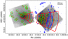 |
Fig. 4. A3376 central and western observations in the band 0.5–10 keV. The blue contours represent VLA radio observations. The green circles represent the extracted points sources with r = 1′. The red annular regions are used for the spectral analysis detailed in Table 3. |
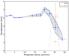 |
Fig. 5. Radial temperature profile for the western region. The gray and blue area represent the CXB and NXB systematic uncertainties. The orange points show the 2T model temperatures at the western radio relic. The dashed gray line is the VLA radio radial profile. |
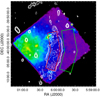 |
Fig. 6. A3376 W1 and W2 NXB subtracted images in the band 0.5–10 keV. The white contours correspond to VLA radio observations. The green and red polygonal regions are the pre and post-shock regions of the western radio relic, respectively. |
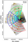 |
Fig. 7. A3376 center, north, east, and south images in the band 0.5–10 keV. The cyan contours represent VLA radio observations. The yellow circles represent the extracted points sources. The green (north), blue (east) and red (south) annular regions are used for the spectral analysis detailed in Tables 6, 5, and 7, respectively. |
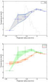 |
Fig. 8. Radial temperature profile for the eastern region (top is east and bottom is north and south). Top: Gray and blue areas represent the CXB and NXB systematic uncertainties. The dashed gray line is the VLA radio radial profile. Bottom: Green and red areas represent the CXB and NXB systematic uncertainties for north and south, respectively. |
3.3. Spectral analysis along the western region
For the spectral analysis of the western region, we have analyzed several annular regions centered on the X-ray emission peak centroid (RA = 6h02m07s.66, Dec = −39°57′42″.74) once the point sources (see green circles in Fig. 4) have been excluded. The regions are a circle in the center with r = 2′ and annuli between 2′–4′, 4′–6′, 6′–9′, 13′–15′, 15′–17′, 17′–19′, 19′–21′, 21′–24′, 24′–27′, and 27′–31′. For all of them, the FI (used energy range 0.5–10 keV) and BI (0.5–7.0 keV) spectra have been fitted simultaneously. We analyzed the NXB subtracted spectra with the normalization Norm, temperature kT and metal abundance Z for the inner region r ≤ 9′ as free parameters. The sky background components have been fixed to the values presented in Table 2.
The best-fit parameters are summarized in Table 3. In general, we obtained a good fit for all regions (C-stat/d.o.f. < 1.2). The resulting radial temperature profile is shown in Fig. 5. It includes in gray and blue the systematic uncertainties due to the CXB fluctuation and NXB, respectively, as mentioned above. The radial profile shows an average temperature of ∼4 keV in the central region of the cluster as found earlier by De Grandi & Molendi (2002), Kawano et al. (2009) and Akamatsu et al. (2012). At r = 20′ the temperature increases slightly to ∼5 keV and drops smoothly to ∼1.4 keV beyond the western radio relic. Although there is a temperature decrease, there is not a clear discontinuity in the temperature at the radio relic. One possible explanation is that the annular region at r = 24′–27′ contains gas from the pre and post relic region, which have two different temperatures. In order to investigate this aspect we included a second cie model in this region. As a result, we obtained two distinct temperatures: kT1 = 4.2 ± 1.3 keV and kT2 = 1.1 ± 0.2 keV (see orange points in Fig. 5) which are consistent with adjacent regions indicating the presence of multi-temperature structure within the extraction region. Therefore, this could be a preliminary indication of a temperature jump in the radio relic area and the possible presence of a shock front.
As a next step, we defined two additional regions in order to obtain the temperature upstream and downstream of the possible X-ray shock (Fig. 6). We introduced a separation of ∼1′ between pre and post-shock region to avoid a possible photon leakage from the brighter region due to limited PSF of XRT (Akamatsu et al. 2015, 2017). The pre-shock region is located beyond the radio relic edge (the green polygonal region in Fig. 6) and the post-shock region is inside the radio relic edge (the red polygonal region in Fig. 6). The resulting best-fit parameters for these pre and post-shock regions are shown in Table 4 and the spectrum of the post-shock region is shown in Fig. 9. In this new analysis, the temperature shows a significant drop from kTpost = 4.22 ± 0.26 keV to kTpre = 1.27 ± 0.29 keV. These ICM temperatures of the pre and post-shock regions agree with previous Suzaku results ( to kTpre = 1.34 ± 0.42 keV, Akamatsu et al. 2012. We discuss the shock properties related to the western radio relic in Sect. 4.3.
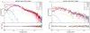 |
Fig. 9. Left: NXB-subtracted spectrum of western post-shock region in the 0.5–10 keV band. Right: eastern post-shock spectrum in the 0.7–7.0 keV band. The FI (black) and BI (red) spectra are fitted with the ICM model together with the CXB and Galactic emission. The ICM is shown in magenta. The LHB, MWH and CXB are represented by green, blue and orange curves, respectively. The ICM, LHB, MWH, and CXB has been represented relative to the BI spectrum. |
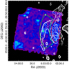 |
Fig. 10. A3376 East NXB subtracted images in the band 0.5–10 keV. The white contours correspond to VLA radio observations. The green and red annular regions are the pre and post-shock regions of the eastern and northern radio relic, respectively. |
3.4. Spectral analysis along the eastern region
In the spectral analysis of the eastern region we have studied three different directions: N, E, and S, corresponding to the observations with the same names (see Table 1). We used annular regions, with the same centroid as the western region (RA = 6h02m07s.66, Dec = −39°57′42″.74), between 2′–4′, 4′–6′, 6′–9′, 9′–12′, 12′–16′ and 16′–20′. Figure 7 shows green regions for N, blue regions for E and red regions for S. We fit the FI (0.7–7.0 keV) and BI (0.7–5.0 keV) spectra simultaneously. We applied the same criteria for the background components and the ICM definition as explained above for the western regions. The best-fit parameters for east, north, and south are summarized in Tables 5, 6, and 7, respectively. In general we obtained a good fit with C-stat/d.o.f. < 1.1 for E and S, and C-stat/d.o.f. < 1.25 for N. Figure 8 shows the radial temperature profile for the three directions. In general, the statistical errors in our data are larger than or of the same order of magnitude as the systematic errors.
The radial temperature profile in the E direction shows a slight increase of the temperature at the center followed by a temperature gradient until ∼1 keV in the cluster outer region. Motivated by a surface brightness discontinuity found at r ∼ 8′ explained in Sect. 4.2, we then analyzed a pre-shock (green annular) and post-shock (red annular) region (see Fig. 10). The best-fit parameters show a decrease from kTpost = 4.71 keV to kTpre = 3.31 keV (Table 8). The spectrum of the post-shock region is shown in Fig. 9. These ICM temperatures are consistent with the ones estimated in the eastern annular regions at r = 6–9′ and r = 9–12′.
For the N direction, we divided the annular regions in two (Na: 350-22.5° and Nb: 22.5-55°) sections to investigate possible azimuthal differences. After the spectral analysis we could not find any significant difference between both sides. Therefore, we have analyzed the full annular regions as shown in Fig. 7. The temperature increases up to ∼5 keV at r = 7.5′ and decreases till ∼1 keV in the cluster outskirts. We investigated pre and post-shock regions at r = 8′, similar to the case of the eastern direction to analyze the extent of the eastern shock, and there are no signs of a temperature drop.
In the S direction, we obtain a radial temperature profile with a central temperature of ∼4 keV and a smooth decrease down to the cluster peripheries. It follows the predicted trend for relaxed galaxy clusters as described by Reiprich et al. (2013). We discuss this behavior in more detail in Sect. 4.1.
4. Discussion of spectral analysis
4.1. ICM temperature profile
The main growing mechanism of galaxy clusters includes the accretion and merging of the surrounding galaxy groups and subclusters. These processes are highly energetic and turbulent, being able to modify completely the temperature structure of the ICM (Markevitch & Vikhlinin 2007). Therefore, this temperature structure contains the signatures of how the cluster has evolved, providing relevant information on the growth and heating history.
There are fewer studies about merging galaxy clusters and the impact of the above events to the ICM temperature structure then about relaxed clusters. A recent compilation of Suzaku observations shows the temperature profile up to cluster outskirts (Reiprich et al. 2013). That review shows that relaxed clusters have a similar behavior near r200 and that the temperature can smoothly drop by a factor of three at the periphery. Moreover, these Suzaku data are consistent with the ICM temperature model of relaxed galaxy clusters proposed by Burns et al. (2010).
Burns et al. (2010) obtained this “universal” profile model based on N-body plus hydrodynamic simulations for relaxed clusters. The scaled temperature profile as a function of normalized radius is given by:![Mathematical equation: $ \begin{aligned} \frac{T}{T_{\mathrm{avg}}} \,{=}\,A\bigg [1+B\left(\frac{r}{r_{200}}\right)\bigg ]^\beta , \end{aligned} $](/articles/aa/full_html/2018/10/aa32496-17/aa32496-17-eq5.gif) (4)
(4)
where the best-fit parameters are A = 1.74 ± 0.03, B = 0.64 ± 0.10 and β = 3.2 ± 0.4. Tavg is the average X-ray weighted temperature between 0.2–1.0r200.
In Fig. 11 we compare Burns’ radial profile with the radial temperature profile of A3376 normalized with ⟨kT⟩ = 4.2 keV (⟨kTx⟩ up to 0.3r200, (Reiprich et al. 2009) and r200 ∼ 1.76 Mpc derived from Henry et al. (2009). The western direction shows an enhancement of the temperature compared with the relaxed profile and a sharp drop close to ∼0.7r200. This is a hint for the presence of a shock front and shock heating of the ICM at these radii. A similar, but less pronounced, behavior is found for the north and east, being the temperature excess higher for the north. In both cases, the temperature shows a decrease around ∼0.3r200, where the eastern radio relic is located, with a steeper temperature profile than relaxed clusters. In the north, the large statistical errors and the weakness of the signal limit the detection of a temperature jump, and therefore, the possible evidence for a shock front. Deeper observations are needed to constrain this temperature structure in more detail. On the other hand, the southern direction seems to follow the profile of relaxed clusters. This is expected because there is no radio emission in this direction.
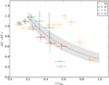 |
Fig. 11. Normalized radial temperature profile of A3376 compared with relaxed clusters. The dashed line represents the Burns et al. (2010) universal profile and the gray area shows its standard deviation. The orange, green, blue and red crosses are the scaled data for the west, north, east, and south directions, respectively. We have shifted these scaled data of the different directions in r/r200 for clarity purpose. |
4.2. X-ray surface brightness profiles
In order to confirm the evidence of bow shocks at the western and eastern regions, we analyzed the radial X-ray surface brightness profile from the center of A3376 using the XMM-Newton observations. The SB was determined in the 0.3–2.0 keV band excluding the Al line at ∼1.5 keV. Point sources with a flux higher than Sc = 10−17 W m−2 were removed (for more details see Sect. 3.2) and the X-ray image was corrected for exposure and background. The sky background components derived from Q0551-3637 (see Table 2) have been adopted together with the instrumental background for the background correction. The surface brightness profile was extracted in circular pie shaped sectors (see sectors in Fig. 12) and fitted with PROFFIT v1.47 (Eckert et al. 2011). We adopted a broken power-law density profile to describe the SB profile. Therefore, assuming spherical symmetry, the density distribution is given by (5)
(5)
where n0 is the model density normalization, α1 and α2 are the power-law indices, r is the radius from the center of the sector and rsh is the shock putative distance. At the location of the SB discontinuity n2, the post-shock (downstream) density is higher by a factor of C = n2/n1 compared with n1, pre-shock (upstream) density. This factor C is known as the compression factor. In the X-ray SB fitting, we left all these model parameters free to vary.
The radial SB profile across the western radio relic is shown in Fig. 13. The SB was accumulated in circularly shaped sectors to match the outer edge of the radio relic from an angle of 230° to 280° (measured counter-clockwise) for r = 21–28′. The data were rebinned to reach a minimum signal-to-noise ratio (S/N) of four. The best-fitting broken power-law model is shown as the blue line with C-stat/d.o.f. ∼ 1.2. It presents a break inside the radio relic at rsh∼ 23′ (measured from the X-ray emission peak centroid) and the compression factor is C = 1.9 ± 0.4. If we apply the PSF modeling of XMM-Newton as described in Appendix C of Eckert et al. (2016a) for a more accurate estimate of the density profile, then the density jump increases to C = 2.1 ± 0.6. We have additionally evaluated different elliptical shaped sectors to adjust them to the relic shape. They have eccentricities of ε = 0.6 and ε = 0.73. The compression factors obtained in both cases are lower than for the circular sector, C = 1.7 ± 0.3 and C = 1.5 ± 0.4, respectively. The different radii for the SB discontinuity compared with the temperature jump could be caused by the Suzaku PSF ∼2′.
The obtained value of C = 2.1 ± 0.6 is consistent within the 1σ uncertainty bounds with the value in Table 9, C = 2.9 ± 0.3, although it shows a slightly lower value. This could possibly be explained because of the difficulty to model the multi-component background in the lack of any sky region where it cannot be spatially separated from the ICM. Therefore, the background modeling can play also an important role in the SB profiles located at the outskirts. Future observations with the Athena satellite could provide an explanation to this issue.
We obtained the radial SB profile along the E direction for circular sectors between 35° to 125° with the center at the X-ray emission peak. The data were rebinned to have a minimum S/N ∼ 8. For radii larger than 12′ the SB emission is low and is background dominated. For this reason, we selected the range 4–12′ for the fitting. The best-fitting broken power-law model is shown in Fig. 14 as a blue line with C-stat/d.o.f. ∼ 1.4. The SB profile contains an edge at r∼ 8′ and the compression factor is C = 1.9 ± 0.5, after applying the same PSF modeling as for the western SB profile. Because the radial profile of the radio relic azimutally averages various features (see VLA radio contours in Figs. 10 and 12), this edge appears to be located ahead of a secondary peak in the radio relic profile. It seems to be associated to the “notch” described by Paul et al. (2011) and Kale et al. (2012).
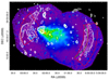 |
Fig. 12. XMM-Newton image in the 0.5–10 keV band of A3376. The white contours correspond to VLA radio observations. The red sectors are used to extract the X-ray SB profile in the E and W directions. The dashed red line represents the circular (ε = 0) shaped sector used for the SB profiles. The magenta and green lines are the elliptical shaped sectors with ε = 0.60 and ε = 0.73, respectively. |
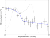 |
Fig. 13. Radial X-ray surface brightness profile across the western radio relic in the 0.3–2.0 keV band using XMM-Newton observations. The profile is corrected for vignetting and background level, and point sources have been removed. The solid blue curve is the best-fit model and the gray dashed line is the VLA scaled radio emission. The data were rebinned to reach a minimum S/N of four and C-stat/d.o.f. ∼ 1.2. |
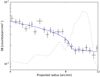 |
Fig. 14. Radial X-ray surface brightness profile across the eastern radio relic in the 0.3–2.0 keV band using XMM-Newton observations. Same as Fig. 13, with a minimum S/N of eight and C-stat/d.o.f. ∼ 1.4. |
4.3. Shock jump conditions and properties
The density (surface brightness) and temperature discontinuities found along the western and eastern directions form evidence for a shock front co-spatial with the western relic (Fig. 13 and Table 4) and the “notch” radio structure in the east (Fig. 14 and Table 8), respectively. Here, we calculate the shock properties in the western and eastern directions based on our Suzaku observations. The Mach number (ℳ) and compression factor (C) can be assessed from the Rankine-Hugoniot jump condition (Landau & Lifshitz 1959) assuming that all of the dissipated shock energy is thermalized and the ratio of specific heats (the adiabatic index) is γ = 5/3: (6)
(6)
 (7)
(7)
where n is the electron density, and the indices 2 and 1 corresponds to post-shock and pre-shock regions, respectively. Table 9 shows the Mach numbers and compression factors derived from the observed temperature jumps. The Mach numbers are in good agreement with the simulations of Machado & Lima Neto (2013) and ℳW is consistent with previous Suzaku results obtained by Akamatsu et al. (2012) (ℳW = 3.0 ± 0.5). The Mach numbers estimated from the surface brightness discontinuities described in the previous sections are ℳWSB ∼ 1.3–2.5 and ℳESB ∼ 1.7 ± 0.4. Both values are consistent with the value present in Table 9 within 1σ error. The presence of shocks with ℳ ≳3.0 is uncommon in galaxy clusters, only four other clusters have been found with such a high Mach number (“El Gordo”, Botteon et al. 2016b; A665, Dasadia et al. 2016a; CIZA J224.8+5301, Akamatsu et al. 2015; “Bullet”, Shimwell et al. 2015).
The sound speed at the pre-shock regions is cs, W ∼ 570 km s−1 and cs, E ∼ 940 km s−1, assuming cs =  where μ = 0.6. The shock propagation speeds vshock = ℳ ⋅ cs for the western and eastern directions are vshock, W ∼ 1630 ± 220 km s−1 and vshock, E ∼ 1450 ± 150 km s−1, respectively. These velocities are consistent with previous work for A3376 W (Akamatsu et al. 2012). However, the shock velocities are smaller than in other galaxy clusters with ℳ ∼ 2–3 as the Bullet cluster (4500 km s−1, Markevitch et al. 2002), CIZA J2242.8+530 (2300 km s−1, Akamatsu et al. 2017) and A520 (2300 km s−1, Markevitch et al. 2005).
We have compiled the shock velocities, vshock, for several merging galaxy clusters as shown in Fig. 15. Black points represent data taken directly from the literature and the gray points are calculated from ℳ and kT1. Blue and red crosses are the western and eastern shock velocities, respectively. Figure 15 shows shock velocities as a function of average temperature of the system. To investigate the origin of driving force of the shock structure, we have examined a prediction from self-similar relationship: vshock = A * ⟨kT⟩(3/2) + B, where A = 70 ± 16 and B = 550 ± 270, see orange line. As we expected, most of samples can be explained with this formula, which means that the main driving force of the merging activity is the gravitational potential of the system and no additional physics. Further sample of shocks and proper gravitational mass estimates will enable us to extend this type of examination.
Shock properties at the western and eastern radio relics.
4.4. Mach number from X-ray and radio observations
After the first confirmation by Finoguenov et al. (2010) of a clear correlation between X-ray shock fronts and radio relics in A3667, many other observations have revealed a possible relation between them (Macario et al. 2011; Mazzota et al. 2011; Akamatsu & Kawahara 2013). As explained in the introduction, the X-ray shock fronts may accelerate charged particles up to relativistic energies via diffusive shock acceleration (DSA, Drury 1983; Blandford & Eichler 1987), which in the presence of a magnetic field can generate synchrotron emission. The acceleration efficiency of this mechanism is low for shocks with ℳ < 10 and might not be sufficient to produce the observed radio spectral index (Kang et al. 2012; Pinzke et al. 2013). Therefore, alternative scenarios have been proposed like the presence of a fossil population of nonthermal electrons and re-acceleration of these electrons by shocks (Bonafede et al. 2014; van Weeren et al. 2017) or the electron re-acceleration by turbulence (Fujita et al. 2015; Kang 2017).
DSA is based on first order Fermi acceleration, considering that there is a stationary and continuous injection, which accelerates relativistic electrons following a power-law spectrum n(E)dE ∼ E−pdE with p = (C + 2)/(C − 1), α = − (p − 1)/2 where p is the power-law index and α is the radio spectral index for Sv ∝ vα. The radio Mach number can be calculated from the injection spectral index as (8)
(8)
For A3376 two radio observations exist in addition to the Very Large Array (VLA) observations by Bagchi et al. (2006): Giant Metrewave Radio Telescope, GMRT, 150 and 325 MHz: Kale et al. (2012) and Murchison Widefield Array, MWA, 80−215 MHz: George et al. (2015). Kale et al. (2012) describe in detail the morphology of the E and W relics. They consider the DSA mechanism assuming that the synchrotron and inverse Compton losses have not affected the spectrum. Therefore, for the injected spectral index calculation they use the flattest spectrum in the outer edge of the spectral index map for 325–1400 MHz. Their results are αE = –0.70 ± 0.15, which implies ℳE = 3.31 ± 0.29; and αW = –1.0 ± 0.02 with ℳW = 2.23 ± 0.40. In this case, there are slight differences between the Mach number assessed from the X-ray and radio observations. George et al. (2015) have derived the integrated spectral indices of the eastern and western relic using the GMRT, MWA and VLA observations (see their Fig. 3) obtaining αE = –1.37 ± 0.08 and αW = –1.17 ± 0.06, which give the Mach numbers, assuming αint = αinj – 0.5, ℳE = 2.53 ± 0.23 and ℳW = 3.57 ± 0.58, respectively. However, due to the low angular resolution of MWA, they can only resolve the integrated spectral index and not the injected one. For this reason, we have decided not to use the George et al. (2015) results for this study.
The differences between ℳR and ℳX are not only present in this galaxy cluster. Figure 16 includes several systems with similar behavior to A3376 (see Table 10), which is shown by a blue cross for A3376 W. A3376 E is not included because the spectral index reported by the radio observations refers to the elongated radio relic and not to the ‘notch’ structure. The orange crosses represent radio data obtained with LOFAR. ℳX of these clusters is derived from the temperature jump and ℳR is calculated using Eq. (8) with the injection spectral index αinj. In addition, some other clusters as A521 (Bourdin et al. 2013; Giacintucci et al. 2008), A2034 (Owers et al. 2014; Shimwell et al. 2016) or ‘El Gordo’ (Botteon et al. 2016b; Lindner et al. 2014); present evidence for a shock front based on the surface brightness jump. In order to remain consistent regarding the method used to derive ℳ (in our case, the temperature jump), we do not include these measurements in Fig. 16. We note that Mach numbers based on the SB jump seem to be smaller than those based on temperature jump (for more details, see Sarazin et al. 2016).
Akamatsu et al. (2017) discuss several possible reasons for the Mach number discrepancies in X-rays and radio. In this study we focus on the radio ageing effect (Pacholczyk 1973; Miniati 2002; Stroe et al. 2014), which can lead to lower radio ℳ compared to X-rays. The electron ageing effect takes places when the relativistic electrons lose their energy via radiative cooling or inverse-Compton scattering after the shock passage in approximately less than ∼107–108 years, which is shorter than the shock life time. As a consequence, the radio spectrum becomes steeper and the integrated spectral index decreases from αint to αinj – 0.5 in DSA model (Pacholczyk 1973; Miniati 2002). Only measurements with high angular resolution and low-frequency are able to measure αinj directly. As a consequence, the calculation of ℳR might be underestimated. Moreover, it is thought that the simple relationship of αint = αinj – 0.5 most likely does not hold for the relics case (Kang & Ryu 2015; Kang & Ryu 2016). In the case of A3376, Kale et al. (2012) showed that the spectral distribution steepens from the outer to the inner edge in the frequency range 325–1400 MHz. However, to avoid the ageing effect they consider only the flattest spectral index as αinj at the outer edge.
We calculated the distance free of ageing effect as d = tloss × vgas, where tloss is the cooling time for relativistic electrons and vgas = vshock/C is the gas velocity. We estimated tloss ∼ 10 − 5 × 10⁷ yr from Eq. (14) of Kang et al. (2012): (9)
(9)
where we assumed a magnetic field of B ∼ 1 μG and vobs = 325 MHz–1.4 GHz. The effective magnetic field is Beff2 = B2 + BCBR2, which includes the equivalent strength of the cosmic background radiation like BCBR = 3.24 μG (1+z)2. The gas velocity is vgas, W∼ 564 km s−1 for the west. Therefore, the distance free of the ageing effects is dW ∼ 58–28 kpc. In the case of assuming a five times higher magnetic field, B ∼ 5 μG, tloss∼ 4 × 10⁷ yr (20 % lower than with B ∼ 1 μG) and for B ∼ 0.2 μG tloss∼ 2 × 10⁷ yr (60 %), for vobs = 1.4 GHz. Therefore, the assumptions of B ∼ 1 μG seems the most conservative one. This distance at 1.4 GHz, 28 kpc, is smaller than the radio beam at same frequency (69″ × 69″ or 65 × 65 kpc) used for the spectral index estimation (Kale et al. 2012). Thus, ℳR may be affected by the ageing effect.
Additionally, the X-ray SB discontinuities in the west and east (see Figs. 13 and 14) do not coincide with the outermost edges of the radio relics. There is significant radio structure outside these SB discontinuities. Therefore, while the DSA mechanism associated to these shocks is assumed to be responsible for the radio emission directly behind the shocks, it cannot explain all radio emission. There might be other shocks further outward, but these are below the detection threshold using current instruments, due to a combination of low spatial resolution (Suzaku) or high background (XMM-Newton), so we cannot test that hypothesis in the present study. Together with the ageing effect discussed before, this might contribute to the difference between the Mach number derived from the X-ray and radio observations.
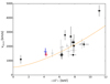 |
Fig. 15. vshock correlation with ⟨kT⟩. The orange line is the best-fit for vshock = A * ⟨kT⟩(3/2) + B. Black crosses represent data taken directly from the literature (Akamatsu & Kawahara 2013; Akamatsu et al. 2015, 2017; Dasadia et al. 2016a; Eckert et al. 2016b; Markevitch et al. 2002, 2005; Russell et al. 2012, 2014; Sarazin et al. 2016). Gray points are the calculated data from ℳ and kT1 (Botteon et al. 2016a; Bourdin et al. 2013; Macario et al. 2011; Ogrean & Brüggen 2013; Owers et al. 2014; Sarazin et al. 2016; Trasatti et al. 2015) as explained in the text. Blue and red crosses correspond to the W and E shocks of A3376 as obtained in this work, respectively. |
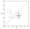 |
Fig. 16. Comparison between Mach number derived from radio observations (ℳR) based on the radio spectral index and the X-ray observations (ℳX). The results for A3376 W is represented by the blue cross. The gray crosses show data for others clusters (see Table 10), orange crosses show recent radio observations done with LOFAR references. The black dashed line is the linear correlation used as reference. |
The cluster sample for our ℳX and ℳR comparison.
4.5. Merger scenario
The N-body hydrodynamical simulations of A3376 by Machado & Lima Neto (2013) predict a merger scenario with two subclusters: one, eastern, which is more compact with four times more concentrated gas than the other, western subcluster. The eastern subcluster has a high initial velocity and is able to cross through the more massive western subcluster, disrupting its core and forming the dense and bright tail. This could be the reason why only one X-ray emission peak is found, probably associated to the BCG2 of the Eastern subcluster in the central region. This scenario is confirmed by the weak lensing analysis of Monteiro-Oliveira et al. (2017), which reveals that the mass peak concentration is in the stripped tail.
From the shock properties, we are able to derive the dynamical age of A3376. Assuming that the western and eastern shocks have traveled from the cluster core to the radio relic location with respective constant velocity (vshock, W ∼ 1630 ± 220 km s−1 and vshock, E ∼ 1450 ± 150 km s−1) and the distance between both shocks is ∼1.9 Mpc, the time required to reach the current position is ∼0.6 Gyr. This value is in good agreement with the previous estimates by Monteiro-Oliveira et al. (2017), George et al. (2015) and Machado & Lima Neto (2013). It might indicate that A3376 is a young merger cluster which is still evolving and following the outgoing scenario as proposed by Akamatsu et al. (2012) and Monteiro-Oliveira et al. (2017).
We also estimated the inclination angle of the line-of-sight with respect to the merging axis, assuming that the galaxies of the infalling (eastern) subcluster are moving together with the shock front. The brightest galaxy of the E subcluster has a z = 0.045591 ± 0.00008 (Smith et al. 2004) and the peculiar velocity with respect to the entire merging cluster (z = 0.0461 ± 0.003, Monteiro-Oliveira et al. 2017) is ∼154 ± 94 km s−1. From the relation θ = arctan(vspec/vshock, E), we estimated θ ∼ 6° ± 4°. This means that the merger axis is close to the plane of sky.
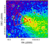 |
Fig. 17. A3376 Chandra background and exposure corrected image in the 0.5–2.0 keV band. The red annular regions are used in the spectral analysis of the cold front and the same pie shaped annuli are used for the SB profile estimation. |
5. Cold front near the center
The Chandra image shown in Fig. 17 reveals an arc-shape edge between 25–140° (measured counter-clockwise), orthogonal to the merging axis in the NE direction. For a refined spatial analysis of this feature, we extracted the X-ray surface brightness profile from the center of A3376 to the E using the Chandra observations (see Table 1) in the 0.5–2.0 keV band. The circular pie annuli used to accumulate the SB profile cover the angle interval 50–120° from the centroid in RA = 6h02m12s.08, Dec = −39°57′18″.53 (same as the red annular sectors of Fig. 17). The same regions are used for the spectral analysis where point sources using the criteria of Sc = 10−17 W m−2 have been excluded. Figure 18 shows the radial SB profile along the E direction. It shows an edge (C = 1.78 ± 0.15) in the SB profile at approximately 150 kpc (∼3′) distance from the X-ray emission peak.
We determined the radial temperature profile using XMM-Newton and Suzaku observations, see Fig. 19, across the E direction for the four annular regions shown in Fig. 17. The temperature rises from ∼3.0 to ∼4.6 keV (Tin/Tout = 0.65 ± 0.08) just outside of the SB edge location based on XMM-Newton observations.
The radial SB and temperature profiles show that the gas is cooler and denser (brighter) inside the edge. Using the density and temperature discontinuities of C = 1.78 ± 0.15 and Tin/Tout = 0.65 ± 0.08, respectively; the pressure jump is Pin/Pout = 1.16 ± 0.17. Therefore, the pressure is almost continuous across the edge, which agrees with the definition of a cold front.
In addition to the two shock fronts described in the previous sections, we found evidence of a sharp edge close to the center associated to a cold front. It delimits the boundaries of a cool and dense gas cloud moving through a hotter ambient gas, which is subject to ram pressure stripping (Markevitch & Vikhlinin 2007; Vikhlinin et al. 2001). Figure 17 shows this case, with the shape of the front perpendicular to the merger axis advancing in the NE direction. Using the temperatures and densities derived from the X-ray image and spectral analysis, we estimated the velocity of the cool gas cloud (Landau & Lifshitz 1959; Vikhlinin et al. 2001; Dasadia et al. 2016b; Ichinohe et al. 2017). We approximated the cool gas as a spherical body advancing into ambient gas. If the cloud moves with supersonic velocity, a shock front could form upstream of the gas cloud. Near the cold front edge the cool gas decelerates to zero velocity at the stagnation point, referred here with the index 0. We also assumed a free stream of gas upstream of the cold front, which is undisturbed and flows free, denoted by index 1. The ratio of pressures in the free stream and the stagnation point can be expressed as a function of the gas cloud speed v (Landau & Lifshitz 1959): (10)
(10)
where γ = 5/3 is the adiabatic index; ℳ1 = v/cs and cs are the Mach number and sound velocity of the free stream, respectively.
The gas parameter at the stagnation point cannot be measured directly, although the stagnation pressure is similar to the gas cloud inside the cold front (Vikhlinin et al. 2001). Therefore we assumed T0 = 3.00 ± 0.27 keV as the temperature inside the cold front and T1 = 4.60 ± 0.80 keV outside the cold front used as the free stream region (Vikhlinin et al. 2001; Sarazin et al. 2016). The density ratio of these regions is calculated from the best-fit parameter of the broken power-law model of Fig. 18, n0/n1 = 3.91 ± 0.75. Thus, the pressure ratio between the inside of the cold front and the outside free stream region is p0/p1 = 2.6 ± 0.6, which corresponds to ℳ1 = 1.2 ± 0.2 in the free stream. Using ccf =  with kT1 = 4.60 keV, ccf = 1100 ± 100 km s−1 and the velocity of the cool gas cloud is vcf = 1300 ± 250 km s−1. This value is consistent with the velocity of the shock front, vshock, E = 1450 ± 150 km s−1, derived in Sect. 4.3.
As explained in Dasadia et al. (2016b), for a rigid sphere the ratio of ds/Rcf, with ds the shock “stand-off” distance and Rcf the radius of curvature of the cold front, depends on ℳ as a function of (ℳ2 − 1)−1 (see Dasadia et al. Fig. 9, Schreier 1982; Vikhlinin et al. 2001; Sarazin 2001). For a shock with ℳE = 1.5 ± 0.1, the shock offset ratio is ds/Rcf ∼ 0.8 ± 0.1, ds ∼ 120 ± 15 kpc (Rcf ∼ 150 kpc). This separation for a rigid sphere is smaller than the distance of ∼300 kpc between the cold front and shock front present in the east. This behavior is the same for most of the observed clusters (Dasadia et al. 2016b). As explained by Sarazin et al. (2016), after the first core passage the shock accelerates toward the periphery of the clusters, while the cool gas is decelerated by gravity and ram pressure. For this reason, the shock is expected to move away from the cold front and the separation between both features might be larger than the rigid sphere model predicts.
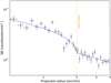 |
Fig. 18. Radial X-ray surface brightness profile across the cold front in the 0.5–2.0 keV band using the Chandra observation. The profile is corrected for exposure and background, and point sources are removed. The solid blue curve is the best-fit model and the vertical orange line is the estimated position of the cold front. |
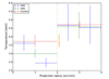 |
Fig. 19. Radial temperature distribution for the red annular regions shown in Fig. 17. Blue and green crosses correspond to XMM-Newton observations and red crosses to Suzaku. The vertical orange line shows the estimated position of the cold front. |
6. Summary
We present a spectral analysis of A3376 in four directions (west, east, north, and south) using Suzaku deep observations and supported by XMM-Newton and Chandra observations. A3376 is a merging galaxy cluster with two shock fronts and one cold front confirmed. One shock is coincident with the radio relic in the west and the other might be associated to the “notch” of the eastern relic. Shocks are moving with a Mach number ℳ ∼ 2–3. The cold front is located at approximately 150 kpc (r ∼ 3′) from the X-ray emission peak at the center and delimits a cool gas cloud moving with v ∼ 1300 km s−1.
We determine the ICM structure up to 0.9r200 in the W, 0.6r200 in the E. We observe a temperature enhancement followed by a drop at ∼0.7r200 for the W and ∼0.5r200 for the E. We confirm temperature and surface brightness discontinuities in both directions. In the west it coincides with the radio relic position and in the east, it is located at 450 kpc (r ∼ 8′). The temperature structure in the south follows the simulated profile of Burns et al. (2010) for relaxed clusters.
We estimate the Mach number based on the temperature jump, being ℳW = 2.8 ± 0.4 and ℳE = 1.5 ± 0.1, for the western and eastern region, respectively. We derive the shock speed velocity as vshock, W ∼ 1630 ± 220 km s−1 and vshock, E ∼ 1450 ± 150 km s−1.
Assuming that the shock fronts are moving with constant velocity, the time since core passage is ∼0.6 Gyr, which is in good agreement with the N-body hydrodynamical simulations of Machado & Lima Neto (2013), and with earlier multiwavelength analyses of George et al. (2015) and Monteiro-Oliveira et al. (2017). Combining the eastern shock velocity and the peculiar velocity of the eastern brightest galaxy let us infer that the merger axis is close to the plane of the sky.
We compare the Mach numbers inferred from the temperature discontinuities with those derived from radio observations assuming the DSA mechanism. Not all the clusters present a consistent correlation between X-ray and radio Mach numbers. For A3376 the Mach number for the western relic estimated by Kale et al. (2012) is consistent with our result.
Acknowledgments
The authors thank the anonymous referee for constructive comments and suggestions. The authors also thank Dr. R. Kale for providing the VLA radio data. I.U. thanks H. Martínez-Rodríguez for his support in the initial stage of this work. H.A. acknowledges the support of NWO via Veni grant. T.O. and Y.I. acknowledge support by JSPS KAKENHI Grant Numbers 26220703 and 15H03642. SRON is supported financially by NWO, the Netherlands Organization for Scientific Research. This work is based on observations obtained with XMM-Newton, an ESA science mission with instruments and contributions directly funded by ESA member states and the USA (NASA).
References
- Akamatsu, H., & Kawahara, H. 2013, PASJ, 65, 16 [NASA ADS] [CrossRef] [Google Scholar]
- Akamatsu, H., Takizawa, M., Nakazawa, K., et al. 2012, PASJ, 64, [Google Scholar]
- Akamatsu, H., Inoue, S., Sato, T., et al. 2013, PASJ, 65, 89 [NASA ADS] [Google Scholar]
- Akamatsu, H., van Weeren, R. J., Ogrean, G. A., et al. 2015, A&A, 582, A20 [Google Scholar]
- Akamatsu, H., Mizuno, M., Ota, N., et al. 2017, A&A, 600, A100 [NASA ADS] [CrossRef] [EDP Sciences] [Google Scholar]
- Bagchi, J., Durret, F., Lima Neto, G. B., & Paul, S. 2006, Science, 314, 791 [NASA ADS] [CrossRef] [PubMed] [Google Scholar]
- Bell, A. R. 1987, MNRAS, 225, 615 [NASA ADS] [Google Scholar]
- Blandford, R., & Eichler, D. 1987, Phys. Rep., 154, 1 [Google Scholar]
- Blanton, E. L., Sarazin, C. L., & McNamara, B. R. 2003, ApJ, 585, 227 [NASA ADS] [CrossRef] [Google Scholar]
- Bonafede, A., Intena, H. T., Brüggen, M., et al. 2014, ApJ, 785, 1 [NASA ADS] [CrossRef] [Google Scholar]
- Botteon, A., Gastaldello, F., Brunetti, G., & Dallacasa, D. 2016a, MNRAS, 460, 84 [Google Scholar]
- Botteon, A., Gastaldello, F., Brunetti, G., & Kale, R. 2016b, MNRAS, 463, 1534 [NASA ADS] [CrossRef] [Google Scholar]
- Bourdin, H., Mazzotta, P., Markevitch, M., Giacintucci, S., & Brunetti, G. 2013, ApJ, 764, 82 [NASA ADS] [CrossRef] [Google Scholar]
- Brüggen, M., Bykov, A., Ryu, D., & Röttgering, H. 2012, Space Sci. Rev., 166, 187 [Google Scholar]
- Brunetti, G., & Jones, T. W. 2014, IJMPD, 23, 1430007 [Google Scholar]
- Burns, J. O., Skillman, S. W., & O’Shea, B. W. 2010, ApJ, 721, 1105 [Google Scholar]
- Cappelluti, N., Li, Y., Ricarte, A., et al. 2017, ApJ, 837, 19 [NASA ADS] [CrossRef] [Google Scholar]
- Cash, W. 1979, ApJ, 228, 939 [NASA ADS] [CrossRef] [Google Scholar]
- Dasadia, S., Sun, M., Sarazin, C., et al. 2016a, ApJ, 820, L20 [Google Scholar]
- Dasadia, S., Sun, M., Morandi, A., et al. 2016b, MNRAS, 458, 681 [NASA ADS] [CrossRef] [Google Scholar]
- De Grandi, S., & Molendi, S. 2002, ApJ, 567, 163 [NASA ADS] [CrossRef] [Google Scholar]
- Drury, L. O. 1983, Rep. Prog. Phys., 46, 973 [NASA ADS] [CrossRef] [Google Scholar]
- Durret, F., Perrot, C., Lima Neto, G. B., et al. 2013, A&A, 560, A78 [NASA ADS] [CrossRef] [EDP Sciences] [Google Scholar]
- Eckert, D., Ettori, S., Coupon, J., et al. 2016a, A&A, 592, A12 [NASA ADS] [CrossRef] [EDP Sciences] [Google Scholar]
- Eckert, D., Jauzac, M., Vazza, F., et al. 2016b, MNRAS, 461, 1302 [NASA ADS] [CrossRef] [Google Scholar]
- Eckert, D., Molendi, S., & Paltani, S. 2011, A&A, 526, A79 [NASA ADS] [CrossRef] [EDP Sciences] [Google Scholar]
- Feretti, L., Giovannini, G., Govoni, F., & Murgia, M. 2012, A&ARv, 20, 54 [Google Scholar]
- Ferrari, C., Govoni, F., Schindler, S., Bykov, A. M., & Rephaeli, Y. 2008, Space Sci. Rev., 134, 93 [NASA ADS] [CrossRef] [Google Scholar]
- Finoguenov, A., Sarazin, C. L., Nakazawa, K., Wik, D. R., & Clarke, T. E. 2010, ApJ, 715, 1143 [NASA ADS] [CrossRef] [Google Scholar]
- Fujita, Y., Akamatsu, H., & Kimura, S. S. 2016, PASJ, 68, 34 [NASA ADS] [CrossRef] [Google Scholar]
- Fujita, Y., Tawa, N., Hayashida, K., et al. 2008, PASJ, 60, 343 [Google Scholar]
- Fujita, Y., Takizawa, M., Yamazaki, R., Akamatsu, H., & Ohno, H. 2015, ApJ, 815, 116 [NASA ADS] [CrossRef] [Google Scholar]
- George, L. T., Dwarakanath, K. S., Johnston-Hollitt, M., et al. 2015, MNRAS, 451, 4207 [NASA ADS] [CrossRef] [Google Scholar]
- Giacintucci, S., Venturi, T., Macario, G., et al. 2008, A&A, 486, 347 [NASA ADS] [CrossRef] [EDP Sciences] [Google Scholar]
- Guo, X., Sironi, L., & Narayan, R. 2014a, ApJ, 794, 153 [NASA ADS] [CrossRef] [Google Scholar]
- Guo, X., Sironi, L., & Narayan, R. 2014b, ApJ, 797, 47 [NASA ADS] [CrossRef] [Google Scholar]
- Guo, X., Sironi, L., & Narayan, R. 2017, ApJ, 851, 134 [NASA ADS] [CrossRef] [Google Scholar]
- Henry, J. P., Evrard, A. E., Hoekstra, H., Babul, A., & Mahdavi, A. 2009, ApJ, 691, 1307 [NASA ADS] [CrossRef] [Google Scholar]
- Hindson, L., Johnston-Hollitt, M., Hurley-Walker, N., et al. 2014, MNRAS, 445, 330 [NASA ADS] [CrossRef] [Google Scholar]
- Hoang, D. N., Shimwell, T. W., Stroe, A., et al. 2017, MNRAS, 471, 1107 [NASA ADS] [CrossRef] [Google Scholar]
- Hoshino, A., Henry, J. P., Sato, K., et al. 2010, PASJ, 62, 371 [NASA ADS] [CrossRef] [Google Scholar]
- Ichinohe, Y., Simionescu, A., Werner, N., & Takahashi, T. 2017, MNRAS, 467, 3662 [NASA ADS] [CrossRef] [Google Scholar]
- Ishisaki, Y., Maeda, Y., Fujimoto, R., et al. 2007, PASJ, 59, 113 [NASA ADS] [Google Scholar]
- Itahana, M., Takizawa, M., Akamatsu, H., et al. 2015, PASJ, 67, 113 [NASA ADS] [CrossRef] [Google Scholar]
- Kaastra, J. S. 2017, A&A, 605, A51 [NASA ADS] [CrossRef] [EDP Sciences] [Google Scholar]
- Kaastra, J. S., & Bleeker, J. A. M. 2016, A&A, 587, A151 [NASA ADS] [CrossRef] [EDP Sciences] [Google Scholar]
- Kaastra, J. S., Mewe, R., & Nieuwenhuijzen, H. 1996, in UV and X-ray Spectroscopy of Astrophysical and Laboratory Plasmas, eds. K. Yamashita, & T. Watanabe, 411–414 [Google Scholar]
- Kale, R., Dwarakanath, K. S., Bagchi, J., & Paul, S. 2012, MNRAS, 426, 1204 [NASA ADS] [CrossRef] [Google Scholar]
- Kang, H. 2017, JKAS, 50, 93 [NASA ADS] [Google Scholar]
- Kang, H., & Ryu, D. 2015, ApJ, 809, 186 [NASA ADS] [CrossRef] [Google Scholar]
- Kang, H., & Ryu, D. 2016, ApJ, 823, 13 [NASA ADS] [CrossRef] [Google Scholar]
- Kang, H., Ryu, D., & Jones, T. W. 2012, ApJ, 756, 97 [Google Scholar]
- Kawano, N., Fukazawa, Y., Nishino, S., et al. 2009, PASJ, 61, 377 [NASA ADS] [Google Scholar]
- Koyama, K., Tsunemi, H., Dotani, T., et al. 2007, PASJ, 59, S23 [NASA ADS] [CrossRef] [Google Scholar]
- Kushino, A., Ishisaki, Y., Morita, U., et al. 2002, PASJ, 54, 327 [NASA ADS] [CrossRef] [Google Scholar]
- Landau, L. D., & Lifshitz, E. M. 1959, Fluid mechanics, Course of theoretical physics (Oxford: Pergamon Press) [Google Scholar]
- Lindner, R. R., Baker, A. J., Hughes, J. P., et al. 2014, ApJ, 786, 49 [NASA ADS] [CrossRef] [Google Scholar]
- Lodders, K., Palme, H., & Gail, H. -P. 2009, in Landolt Bömstein (Heidelberg: Springer-Verlag Berlin), 4B, 712 [Google Scholar]
- Macario, G., Markevitch, M., Giacintucci, S., et al. 2011, ApJ, 782, 82 [NASA ADS] [CrossRef] [Google Scholar]
- Machado, R. E. G., & Lima Neto, G. B. 2013, MNRAS, 430, 3249 [NASA ADS] [CrossRef] [Google Scholar]
- Markevitch, M., & Vikhlinin, A. 2007, Phys. Rep., 443, 1 [NASA ADS] [CrossRef] [EDP Sciences] [Google Scholar]
- Markevitch, M., Gonzalez, A. H., David, L., et al. 2002, ApJ, 567, L27 [NASA ADS] [CrossRef] [Google Scholar]
- Markevitch, M., Govoni, F., Brunetti, G., & Jerius, D. 2005, ApJ, 627, 733 [NASA ADS] [CrossRef] [Google Scholar]
- Mazzota, P., Bourdin, H., Giacintucci, S., Markevitch, M., & Venturi, T. 2011, Mem. Soc. Astron. It., 82, 495 [NASA ADS] [Google Scholar]
- Miniati, F. 2002, MNRAS, 337, 199 [NASA ADS] [CrossRef] [Google Scholar]
- Mitsuda, K., Bautz, M., Inoue, H., et al. 2007, PASJ, 59, 1 [Google Scholar]
- Monteiro-Oliveira, R., Neto, G. B. L., Cypriano, E. S., et al. 2017, MNRAS, 468, 4566 [NASA ADS] [CrossRef] [Google Scholar]
- Ogrean, G. A., & Brüggen, M. 2013, MNRAS, 433, 1701 [NASA ADS] [CrossRef] [Google Scholar]
- Ogrean, G. A., Brüggen, M., van Weeren, R. J., Burgmeier, A., & Simionescu, A. 2014, MNRAS, 443, 2463 [NASA ADS] [CrossRef] [Google Scholar]
- Owers, M. S., Nulsen, P. E. J., Couch, W. J., et al. 2014, ApJ, 780, 163 [NASA ADS] [CrossRef] [Google Scholar]
- Pacholczyk, A. G. 1973, Radio astrophysics. Nonthermal processes in galactic and extragalactic sources (Moskva: Mir) [Google Scholar]
- Paul, S., Iapichino, L., Miniati, F., Bagchi, J., & Mannheim, K. 2011, ApJ, 726, 17 [NASA ADS] [CrossRef] [Google Scholar]
- Pinzke, A., Oh, S. P., & Pfrommer, C. 2013, MNRAS, 435, 1061 [NASA ADS] [CrossRef] [Google Scholar]
- Pizzo, R. F., & de Bruyn, A. G. 2009, A&A, 507, 639 [NASA ADS] [CrossRef] [EDP Sciences] [Google Scholar]
- Reiprich, T. H., Hudson, D. S., Zhang, Y. Y., et al. 2009, A&A, 501, 899 [NASA ADS] [CrossRef] [EDP Sciences] [Google Scholar]
- Reiprich, T. H., Basu, K., Ettori, S., et al. 2013, Space Sci. Rev., 177, 195 [NASA ADS] [CrossRef] [EDP Sciences] [Google Scholar]
- Russell, H. R., Mcnamara, B. R., Sanders, J. S., et al. 2012, MNRAS, 423, 236 [NASA ADS] [CrossRef] [Google Scholar]
- Russell, H. R., Fabian, A. C., McNamara, B. R., et al. 2014, MNRAS, 444, 629 [NASA ADS] [CrossRef] [Google Scholar]
- Sarazin, C. L. 2001, Merging Processes in Clusters of Galaxies, Astrophysics and Space Science Library (Dordrecht: Kluwer Academic Publishers), 272, 1 [Google Scholar]
- Sarazin, C. L., Finoguenov, A., Wik, D. R., & Clarke, T. E. 2016, ApJ, submitted, [arXiv:1606.07433] [Google Scholar]
- Schreier, S. 1982, in Compressible Flow (New York: Wiley) [Google Scholar]
- Serlemitsos, P. J., Soong, Y., Chan, K. W., et al. 2007, PASJ, 59, 9 [CrossRef] [EDP Sciences] [Google Scholar]
- Shimwell, T. W., Markevitch, M., Brown, S., et al. 2015, MNRAS, 449, 1486 [NASA ADS] [CrossRef] [Google Scholar]
- Shimwell, T. W., Luckin, J., Br, M., et al. 2016, MNRAS, 459, 277 [NASA ADS] [CrossRef] [Google Scholar]
- Skillman, S. W., Xu, H., Hallman, E. J., et al. 2013, ApJ, 765, [Google Scholar]
- Smith, R. J., Hudson, M. J., Nelan, J. E., et al. 2004, ApJ, 128, 1558 [Google Scholar]
- Storm, E., Vink, J., Zandanel, F., & Akamatsu, H. 2018, MNRAS, 479, 553 [NASA ADS] [Google Scholar]
- Stroe, A., Harwood, J. J., Hardcastle, M. J., & Röttgering, H. J. 2014, MNRAS, 445, 1213 [NASA ADS] [CrossRef] [Google Scholar]
- Struble, M. F., & Rood, H. J. 1999, ApJS, 125, 35 [NASA ADS] [CrossRef] [Google Scholar]
- Tawa, N., Hayashida, K., Nagai, M., et al. 2008, PASJ, 60, 11 [CrossRef] [Google Scholar]
- Thierbach, M., Klein, U., & Wielebinski, R. 2003, A&A, 397, 53 [NASA ADS] [CrossRef] [EDP Sciences] [Google Scholar]
- Trasatti, M., Akamatsu, H., Lovisari, L., et al. 2015, A&A, 575, A45 [NASA ADS] [CrossRef] [EDP Sciences] [Google Scholar]
- Urban, O., Werner, N., Allen, S. W., Simionescu, A., & Mantz, A. 2017, MNRAS, 470, 4583 [NASA ADS] [CrossRef] [Google Scholar]
- van Weeren, R. J., Röttgering, H. J. A., Rafferty, D. A., et al. 2012, A&A, 543, A43 [NASA ADS] [CrossRef] [EDP Sciences] [Google Scholar]
- van Weeren, R. J., Andrade-Santos, F., Dawson, W. A., et al. 2017, Nat. Astron., 1, 5 [NASA ADS] [CrossRef] [Google Scholar]
- van Weeren, R. J., Brunetti, G., Brüggen, M., et al. 2016, ApJ, 818, 204 [NASA ADS] [CrossRef] [Google Scholar]
- Vazza, F., & Brüggen, M. 2014, MNRAS, 437, 2291 [NASA ADS] [CrossRef] [Google Scholar]
- Vikhlinin, A., Markevitch, M., & Murray, S. S. 2001, ApJ, 551, 160 [NASA ADS] [CrossRef] [Google Scholar]
- Vink, J., & Yamazaki, R. 2014, ApJ, 780, 125 [NASA ADS] [CrossRef] [Google Scholar]
- Willingale, R., Starling, R. L. C., Beardmore, A. P., Tanvir, N. R., & O’Brien, P. T. 2013, MNRAS, 431, 394 [NASA ADS] [CrossRef] [Google Scholar]
All Tables
All Figures
|
Fig. 1. Left: Suzaku smoothed image in the 0.5–10 keV band of A3376 (pixel = 8″ and Gausssian 2-D smooth σ = 16″). The white boxes represent the Suzaku XIS FOVs for the C, W1, W2, N, E and S observations listed in Table 1. BCG1 is shown as a black cross and BCG2 as a blue cross. Right: XMM-Newton image in the 0.5–10 keV band of A3376. The white contours correspond to VLA radio observations kindly provided by Dr. R. Kale. |
| In the text | |
|
Fig. 2. Correction of the XIS1 excess in the outer region of the E observation of A3376. The best-fit ICM spectrum is shown as a blue line. The Suzaku XIS BI spectra are shown without (red) and with (green) a 13% increase in the NXB level, respectively. |
| In the text | |
|
Fig. 3. Q0551-3637 spectrum used for the sky background estimation. The Suzaku XIS FI, BI, the LHB, MWH and CXB components are shown in black, red, green, blue, and orange, respectively. The LHB, MWH, and CXB have been represented relative to the BI spectrum. |
| In the text | |
|
Fig. 4. A3376 central and western observations in the band 0.5–10 keV. The blue contours represent VLA radio observations. The green circles represent the extracted points sources with r = 1′. The red annular regions are used for the spectral analysis detailed in Table 3. |
| In the text | |
|
Fig. 5. Radial temperature profile for the western region. The gray and blue area represent the CXB and NXB systematic uncertainties. The orange points show the 2T model temperatures at the western radio relic. The dashed gray line is the VLA radio radial profile. |
| In the text | |
|
Fig. 6. A3376 W1 and W2 NXB subtracted images in the band 0.5–10 keV. The white contours correspond to VLA radio observations. The green and red polygonal regions are the pre and post-shock regions of the western radio relic, respectively. |
| In the text | |
|
Fig. 7. A3376 center, north, east, and south images in the band 0.5–10 keV. The cyan contours represent VLA radio observations. The yellow circles represent the extracted points sources. The green (north), blue (east) and red (south) annular regions are used for the spectral analysis detailed in Tables 6, 5, and 7, respectively. |
| In the text | |
|
Fig. 8. Radial temperature profile for the eastern region (top is east and bottom is north and south). Top: Gray and blue areas represent the CXB and NXB systematic uncertainties. The dashed gray line is the VLA radio radial profile. Bottom: Green and red areas represent the CXB and NXB systematic uncertainties for north and south, respectively. |
| In the text | |
|
Fig. 9. Left: NXB-subtracted spectrum of western post-shock region in the 0.5–10 keV band. Right: eastern post-shock spectrum in the 0.7–7.0 keV band. The FI (black) and BI (red) spectra are fitted with the ICM model together with the CXB and Galactic emission. The ICM is shown in magenta. The LHB, MWH and CXB are represented by green, blue and orange curves, respectively. The ICM, LHB, MWH, and CXB has been represented relative to the BI spectrum. |
| In the text | |
|
Fig. 10. A3376 East NXB subtracted images in the band 0.5–10 keV. The white contours correspond to VLA radio observations. The green and red annular regions are the pre and post-shock regions of the eastern and northern radio relic, respectively. |
| In the text | |
|
Fig. 11. Normalized radial temperature profile of A3376 compared with relaxed clusters. The dashed line represents the Burns et al. (2010) universal profile and the gray area shows its standard deviation. The orange, green, blue and red crosses are the scaled data for the west, north, east, and south directions, respectively. We have shifted these scaled data of the different directions in r/r200 for clarity purpose. |
| In the text | |
|
Fig. 12. XMM-Newton image in the 0.5–10 keV band of A3376. The white contours correspond to VLA radio observations. The red sectors are used to extract the X-ray SB profile in the E and W directions. The dashed red line represents the circular (ε = 0) shaped sector used for the SB profiles. The magenta and green lines are the elliptical shaped sectors with ε = 0.60 and ε = 0.73, respectively. |
| In the text | |
|
Fig. 13. Radial X-ray surface brightness profile across the western radio relic in the 0.3–2.0 keV band using XMM-Newton observations. The profile is corrected for vignetting and background level, and point sources have been removed. The solid blue curve is the best-fit model and the gray dashed line is the VLA scaled radio emission. The data were rebinned to reach a minimum S/N of four and C-stat/d.o.f. ∼ 1.2. |
| In the text | |
|
Fig. 14. Radial X-ray surface brightness profile across the eastern radio relic in the 0.3–2.0 keV band using XMM-Newton observations. Same as Fig. 13, with a minimum S/N of eight and C-stat/d.o.f. ∼ 1.4. |
| In the text | |
|
Fig. 15. vshock correlation with ⟨kT⟩. The orange line is the best-fit for vshock = A * ⟨kT⟩(3/2) + B. Black crosses represent data taken directly from the literature (Akamatsu & Kawahara 2013; Akamatsu et al. 2015, 2017; Dasadia et al. 2016a; Eckert et al. 2016b; Markevitch et al. 2002, 2005; Russell et al. 2012, 2014; Sarazin et al. 2016). Gray points are the calculated data from ℳ and kT1 (Botteon et al. 2016a; Bourdin et al. 2013; Macario et al. 2011; Ogrean & Brüggen 2013; Owers et al. 2014; Sarazin et al. 2016; Trasatti et al. 2015) as explained in the text. Blue and red crosses correspond to the W and E shocks of A3376 as obtained in this work, respectively. |
| In the text | |
|
Fig. 16. Comparison between Mach number derived from radio observations (ℳR) based on the radio spectral index and the X-ray observations (ℳX). The results for A3376 W is represented by the blue cross. The gray crosses show data for others clusters (see Table 10), orange crosses show recent radio observations done with LOFAR references. The black dashed line is the linear correlation used as reference. |
| In the text | |
|
Fig. 17. A3376 Chandra background and exposure corrected image in the 0.5–2.0 keV band. The red annular regions are used in the spectral analysis of the cold front and the same pie shaped annuli are used for the SB profile estimation. |
| In the text | |
|
Fig. 18. Radial X-ray surface brightness profile across the cold front in the 0.5–2.0 keV band using the Chandra observation. The profile is corrected for exposure and background, and point sources are removed. The solid blue curve is the best-fit model and the vertical orange line is the estimated position of the cold front. |
| In the text | |
|
Fig. 19. Radial temperature distribution for the red annular regions shown in Fig. 17. Blue and green crosses correspond to XMM-Newton observations and red crosses to Suzaku. The vertical orange line shows the estimated position of the cold front. |
| In the text | |
Current usage metrics show cumulative count of Article Views (full-text article views including HTML views, PDF and ePub downloads, according to the available data) and Abstracts Views on Vision4Press platform.
Data correspond to usage on the plateform after 2015. The current usage metrics is available 48-96 hours after online publication and is updated daily on week days.
Initial download of the metrics may take a while.