| Issue |
A&A
Volume 617, September 2018
|
|
|---|---|---|
| Article Number | A130 | |
| Number of page(s) | 27 | |
| Section | Extragalactic astronomy | |
| DOI | https://doi.org/10.1051/0004-6361/201833053 | |
| Published online | 02 October 2018 | |
The AKARI 2.5–5 micron spectra of luminous infrared galaxies in the local Universe⋆
1
Univ. Lyon 1, ENS de Lyon, CNRS, Centre de Recherche Astrophysique de Lyon (CRAL) UMR5574, 69230 Saint-Genis-Laval, France
e-mail: hanae.inami@univ-lyon1.fr
2
Infrared Processing and Analysis Center, Caltech, 1200 E. California Blvd., Pasadena, CA 91125, USA
3
Institute of Space and Astronautical Science, Japan Aerospace Exploration Agency, Japan
4
Institute for Astronomy, Astrophysics, Space Applications & Remote Sensing, National Observatory of Athens, 15236 Penteli, Greece
5
University of Crete, Department of Physics, 71003 Heraklion, Greece
6
Núcleo de Astronomía de la Facultad de Ingeniería, Universidad Diego Portales, Av. Ejército Libertador 441, Santiago, Chile
7
Department of Astronomy, University of Virginia, PO Box 400325, Charlottesville, VA 22904, USA
8
National Radio Astronomy Observatory, 520 Edgemont Rd., Charlottesville, VA 22903, USA
9
Academia Sinica, Institute of Astronomy and Astrophysics, 11F of Astronomy-Mathematics Building, National Taiwan University, No.1, Sec. 4 Roosevelt Rd., 10617 Taipei, Taiwan
10
Glendale Community College, 1500 North Verdugo Road, Glendale, CA 91208, USA
Received:
19
March
2018
Accepted:
11
June
2018
We present AKARI 2.5–5 μm spectra of 145 local luminous infrared galaxies (LIRG; LIR ≥ 1011 L⊙) in the Great Observatories All-sky LIRG Survey (GOALS). In all of the spectra, we measure the line fluxes and equivalent widths (EQWs) of the polycyclic aromatic hydrocarbon (PAH) at 3.3 μm and the hydrogen recombination line Brα at 4.05 μm, with apertures matched to the slit sizes of the Spitzer low-resolution spectrograph and with an aperture covering ∼95% of the total flux in the AKARI two-dimensional (2D) spectra. The star formation rates (SFRs) derived from the Brα emission measured in the latter aperture agree well with SFRs estimated from LIR, when the dust extinction correction is adopted based on the 9.7 μm silicate absorption feature. Together with the Spitzer Infrared Spectrograph (IRS) 5.2–38 μm spectra, we are able to compare the emission of the PAH features detected at 3.3 μm and 6.2 μm. These are the two most commonly used near/mid-infrared indicators of starburst or active galactic nucleus (AGN) dominated galaxies. We find that the 3.3 μm and 6.2 μm PAH EQWs do not follow a linear correlation and at least a third of the galaxies classified as AGN-dominated sources using the 3.3 μm feature are classified as starbursts based on the 6.2 μm feature. These galaxies have a bluer continuum slope than galaxies that are indicated to be starburst-dominated by both PAH features. The bluer continuum emission suggests that their continuum is dominated by stellar emission rather than hot dust. We also find that the median Spitzer/IRS spectra of these sources are remarkably similar to the pure starburst-dominated sources indicated by high PAH EQWs in both 3.3 μm and 6.2 μm. Based on these results, we propose a revised starburst/AGN diagnostic diagram using 2–5 μm data: the 3.3 μm PAH EQW and the continuum color, Fν(4.3 μm)/Fν(2.8 μm). We use the AKARI and Spitzer spectra to examine the performance of our new starburst/AGN diagnostics and to estimate 3.3 μm PAH fluxes using the James Webb Space Telescope (JWST) photometric bands in the redshift range 0 < z < 5. Of the known PAH features and mid-infrared high ionization emission lines used as starburst/AGN indicators, only the 3.3 μm PAH feature is observable with JWST at z > 3.5, because the rest of the features at longer wavelengths fall outside the JWST wavelength coverage.
Key words: galaxies: starburst / galaxies: active / infrared: galaxies
Full Table 1 and data associated to Fig. 9 are only available at the CDS via anonymous ftp to cdsarc.u-strasbg.fr (130.79.128.5) or via http://cdsarc.u-strasbg.fr/viz-bin/qcat?J/A+A/617/A130
© ESO 2018
 Open Access article, published by EDP Sciences, under the terms of the Creative Commons Attribution License (http://creativecommons.org/licenses/by/4.0), which permits unrestricted use, distribution, and reproduction in any medium, provided the original work is properly cited.
1. Introduction
The rest-frame 2–5 μm spectra of galaxies provide a wealth of diagnostic power, since they can be used to trace hot dust, small grain dust emission, ionizing flux, and starlight. Starburst-dominated galaxies show a strong polycyclic aromatic hydrocarbon (PAH) emission feature at 3.3 μm (e.g., Genzel & Cesarsky 2000; Imanishi et al. 2010, whereas galaxies with an obscured active galactic nucleus (AGN) show a rising (power law) continuum (e.g., Armus et al. 2007; Yamada et al. 2013). The Brα hydrogen recombination line at 4.05 μm provides a direct measure of the ionizing radiation and thus star formation rate. The absorption features of H2O (3.05 μm) ice, CO2 (4.27 μm) ice, and CO ice and gas (4.67 μm) may be present as well. The AKARI Infrared Satellite (Murakami et al. 2007) performed an all-sky imaging survey in the mid-(9 and 18 μm, Ishihara et al. 2010) and far-infrared (65, 90, 140, and 160 μm, Doi et al. 2015; Takita et al. 2015), but it also had the capability to carry out pointed observations using the infrared camera (IRC) covering 2.5–5 μm at a spectral resolving power of R ∼ 120 (IRC; Onaka et al. 2007).
In infrared luminous galaxies with a dominant central AGN, hot dust (∼1000 K) emission can dominate the near-infrared continuum. The 2.5–5 μm coverage of AKARI facilitates measurements of the relative amounts of hot, warm, and cold dust via comparison to Spitzer mid- and far-infrared data. The PAH emission features are excited by individual ultraviolet (UV) photons, and therefore they are a direct probe of star formation (e.g., Peeters et al. 2004) and are prevalent in star-forming galaxies (Smith et al. 2007). In addition, the PAH features in starburst-dominated galaxies are an important diagnostic of the dust grain properties. For example, weak PAH emission at 3.3 μm, relative to other mid-infrared PAH features (e.g., 7.7 μm), suggests ionization of the small dust grains (Draine & Li 2007). On the other hand, PAH features are invariably absent from the spectra of AGN, which have very hard radiation fields and lack photo-dissociation regions (PDRs, e.g., Laurent et al. 2000; Weedman et al. 2005). For the upcoming James Webb Space Telescope (JWST), the 3.3 μm PAH emission feature will be the only PAH feature observable at z > 3.5. It is, therefore, important to characterize this starburst/AGN diagnostic feature in a large unbiased sample in the local Universe and to quantitatively tie the diagnostic power of this feature to the stronger and more commonly used mid-infrared PAH features that have been used to probe the physics of active starburst galaxies for over two decades.
A large number of studies, some of which include local luminous infrared galaxies (LIRG; LIR ≥ 1011 L⊙), have explored some of the properties of the 3.3 μm PAH, Brα, and hot dust detected with the AKARI spectrograph. For example, these features were used to investigate the starburst/AGN diagnostics of LIRGs and to discuss the properties of starbursts and AGN (Imanishi et al. 2008, 2010; Lee et al. 2012). Woo et al. (2012) focused on Type I AGN and found that the AGN activity is directly related to the nuclear starburst but not the global star formation of the host galaxy. In addition, as a potential star formation rate (SFR) indicator, 3.3 μm PAH emission was compared against the total infrared emission (Kim et al. 2012; Yamada et al. 2013; Yano et al. 2016; Murata et al. 2017). The 3.3 μm PAH and infrared luminosities correlate well up to 1011 L⊙, then break down. However, most of these studies have not directly compared the key diagnostic features over the entire mid-infrared range by combining the AKARI data with those taken with the infrared spectrograph (IRS) on the Spitzer Space Telescope (Houck et al. 2004), which covered the 5–38 μm range, and for which large studies of starbursts and AGN have been published (e.g., Brandl et al. 2006; Gallimore et al. 2010; Haan et al. 2011; Stierwalt et al. 2013, 2014; Shipley et al. 2016). In this paper, we use aperture-matched AKARI and Spitzer/IRS spectra of a sample of 145 local LIRGs to further calibrate the 3.3 μm PAH feature diagnostics, and set the stage for understanding the spectroscopic and photometric observations of this feature in high-redshift galaxies with JWST.
Our 145 local LIRG targets are taken from the Great Observatories All-sky LIRG Survey (GOALS; Armus et al. 2009). The original intention was to observe the complete GOALS sample with AKARI, but unfortunately the mission ended in the middle of the project due to the depletion of the liquid helium coolant. The entire sample of GOALS galaxies (nuclei) and the subsample in this work cover the same log(LIR/L⊙) range of 11.00–12.57, but with mean (median) values of 11.48 (11.40) and 11.60 (11.61), respectively. The ranges of luminosity distances (DL) are 15.9–400.0 Mpc and 17.9–395.0 Mpc with mean (median) values of 115.1 Mpc (95.2 Mpc) and 132.0 Mpc (117.5 Mpc), respectively. The GOALS sample in total contains 178 LIRG and 22 ultra luminous infrared galaxy (ULIRG, LIR ≥ 1012 L⊙) systems in the local Universe. These objects are a flux limited sample drawn from the IRAS1 Revised Bright Galaxy Sample (RBGS; Sanders et al. 2003), which covers galactic latitudes greater than 5° and includes 629 extragalactic objects with 60 μm flux densities greater than 5.24 Jy. Although LIRGs are not common in the local Universe, their number density increases rapidly with redshift at least up to z ∼ 3 and their star formation rate density dominates at z ∼ 2–3, the peak of galaxy formation in the Universe (e.g., Madau & Dickinson 2014). Thus, observations of local LIRGs can help improve our understanding of obscured star formation and black hole growth at all epochs. Since the PAH features are often very strong (e.g., Smith et al. 2007), and easily seen at high redshifts even in low-resolution spectra when no other features are visible, it is critically important to assess their diagnostic power across the entire infrared spectral regime in local galaxies, where high signal-to-noise, multi-wavelength data can be brought to bear to understand the underlying heating mechanisms.
In this study, we combine the AKARI 2.5–5 μm spectra and the Spitzer 5.2–38 μm spectra to investigate the nuclear energy sources, starburst ages, star formation rates, gas ionization, and dust properties of local LIRGs. We will also report on possible diagnostics for both local and high redshift galaxies using JWST observations of this important spectral region. This paper is organized as follows: the AKARI observations are described in Sect. 2, followed by the data reduction and analysis in Sect. 3. The AKARI spectra and derived properties with the Spitzer data are shown in Sect. 4. We present our interpretation of the results in Sect. 5. We also briefly discuss how one could observe these targets with JWST. The summary and conclusions are given in Sect. 6. A cosmology of ΩΛ = 0.72, Ωm = 0.28, H0 = 70 km s−1 Mpc−1 is adopted throughout.
2. Observations
The 2.5–5 μm spectra of 145 GOALS sources were observed with AKARI pointed observations between 2006 October 29 and 2010 February 14 using the infrared camera (IRC; Onaka et al. 2007). The data obtained prior to 2007 August were taken during the cold phase, and the data from after this time were taken in the warm (post-helium) phase mission. The total number of pointings was 385 with the majority obtained with the AGNUL program (54%, PI T. Nakagawa), in addition to 36% from the GOALS program (PI H. Inami), 8% from DTIRC (PI H. Murakami), and the remaining 2% from the BRSFR (PI M. Malkan), EGANS (PI H. Matsuhara), and NULIZ programs (PI H.-S. Hwang). The Np aperture with a size of 1′ × 1′ was used in order to avoid the confusion of spectra from the entire IRC field-of-view (10′ × 10′). The spectral resolving power was R ∼ 120 at 3.5 μm for a point-like source.
Two types of astronomical observation templates (AOT) were employed – IRC04 and IRCZ4. The former was operated during the cold phase mission without dithering and the latter during the warm phase mission with dithering. Both of the AOTs obtained data with the same procedure; taking four spectra, a reference image, and then four or five (depending on if the satellite maneuver happened during the fifth frame) spectra at the end of the sequence. The exposure time for each spectrum was 44.41 s.
3. Data reduction and analysis
The standard data reduction software package provided by Japan Aerospace eXploration Agency (JAXA), the IRC Spectroscopy Toolkit for Phase 3 Data2 (version 20101025), was used to perform dark subtraction, linearity correction, flat correction, background subtraction, wavelength calibration, spectral inclination correction, and spectral response calibration. This package can handle both the cold and warm phase data. Although the number of bad pixels increased dramatically in the post-helium mission due to the elevated detector temperatures, the data quality was uniform enough, for the purposes of this work, to measure the 3.3 μm PAH and Brα line fluxes and the continuum emission. The wavelength accuracy was ∼0.01 μm and the uncertainty in absolute flux calibration was estimated to be ∼10% (Ohyama et al. 2007).
We extracted the one-dimensional (1D) spectrum from the two-dimensional (2D) spectral image using two different methods: (1) the fixed aperture widths of 4.4″ (three pixels) and 10.5″ (seven pixels) and (2) an aperture size covering ∼95% of the total flux in the AKARI 2D spectra. The 1D spectra extracted with the former aperture (1) were used for comparison with the Spitzer IRS short-wavelength low-resolution (SL, 5–14.5 μm) and long-wavelength low-resolution (LL, 14–38 μm) spectra, respectively. The 4.4 ″ width is slightly larger than the SL slit width (3.6″) but matches well the spatial resolution of AKARI over this wavelength range (∼4″), providing an accurate point source spectrum with which to directly compare the Spitzer SL spectra. At the median distance of our sample, 117.5 Mpc, angular sizes of 4.4″ and 10.5″ correspond to physical sizes of 2.4 kpc and 5.7 kpc, respectively. In this work, the LL aperture size is used only when the full range of AKARI and Spitzer 2.5–38 μm spectra is shown in a figure or needed for an analysis. In this case, the scaling factor to correct the mismatch between the SL and LL spectra (due to the different aperture sizes) is applied to the SL spectrum in the same manner as described in Stierwalt et al. (2013). The latter aperture (2) was used to obtain spatially-integrated AKARI measurements suitable for investigating integrated properties of the targets.
The 3.3 μm PAH and Brα line fluxes were obtained by fitting a Gaussian plus a linear function to each feature and its local continuum (see also Fig. 1). The wavelength range and function chosen to fit the continuum varied slightly from source to source to avoid contamination from the broad absorption features, which can be present at 3.05 μm (H2O ice) and 4.67 μm (CO ice and gas). For example, for UGC 05101, a 3° degree Chebyshev polynomial had to be employed instead of a linear fit to the 3.3 μm local continuum because its PAH emission feature sits on the deep absorption features. Typically, the wavelength regions selected for fitting the continuum were 2.65–2.8 μm (shortward of the ice feature) and 3.55–3.7 μm for the PAH emission, and 3.80–4.0 μm and 4.1–4.25 μm for the Brα emission. When an emission line was not detected, a 3σ upper limit was estimated using a Gaussian function with a height three times the local continuum dispersion and with a width equal to the AKARI intrinsic resolution (R ∼ 120).
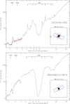 |
Fig. 1. Joined AKARI and Spitzer low-resolution spectra of two typical LIRGs in the sample. The AKARI spectral extraction is performed with the 10.7″ IRS/LL aperture size and the IRS/SL spectra are scaled up to match the LL spectra (see Sect. 3). A starburst-dominated source (CGCG 436-030; top) and an AGN-dominated source (IRAS F08572+3915; bottom) are shown. Their AGN fractions are 8.9 ± 1.8% and 46.6 ± 8.7%, respectively (see Sect. 4.1 and Díaz-Santos et al. 2017). For CGCG 436-030, the fits on the 3.3 μm PAH feature and the Brα line are denoted with red lines. The IRAC 3.6 μm image (1′ × 1′, the same as the AKARI Np FoV size) with the Spitzer IRS SL (red) and LL (blue) apertures overlaid is presented as the inset at the bottom right of each panel. The indicated PAH features in the Spitzer wavelength range are at 6.2, 7.7, 8.6, 11.3, and 12.7 μm in SL, and 16.4 and 17.4 μm in LL. |
The measured line fluxes and AKARI spectra of the entire sample are reported in Table 1 and Appendix B, respectively. Out of the 145 LIRG sample, 3.3 μm PAH emission and Brα emission features were detected in 133 (92%) and 91 (63%) sources, respectively.
4. Results
Two representative, combined AKARI and Spitzer/IRS low-resolution spectra are shown in Fig. 1. One is a starburst-dominated galaxy (CGCG 436-030; upper panel) and the other is an AGN-dominated galaxy (IRAS F08572+3915; lower panel). As expected, the starburst CGCG 436-030 shows pronounced PAH emission features, which are absent in IRAS F08572+3915. Instead, IRAS F08572+3915 has a steeply rising continuum emission contributed by hot and warm dust emission as well as strong absorption features.
There are 15 sources that show large jumps between extracted AKARI and Spitzer/IRS spectra. We exclude these sources from the discussion of the joint spectral analysis, but include them in the discussion of the AKARI spectra alone.
Line flux and EQW of 3.3 μm PAH and Brα and the Fν(4.3 μm)/Fν(2.8 μm) color measured in the 4.4″ radius aperture.
4.1. Starburst and AGN classifications based on PAH features
The most prominent feature in the 2.5–5 μm spectral range covered by AKARI is the emission band at 3.3 μm, which arises from C–H stretching vibrational modes of the PAH carriers. The moderate spectral resolution of our data (R ∼ 120) allows us to separate the 3.3 μm PAH feature from an emission feature at 3.4 μm. The exact nature of the 3.4 μm feature is not entirely clear (Tielens 2008), but it is thought to be a PAH satellite feature (Tokunaga et al. 1991; Sturm et al. 2000). In order to avoid confusion and offer direct comparisons with past work, we employ only the main 3.3 μm PAH emission throughout this paper.
Because the PAH features are stochastically heated by UV photons and the mid-infrared continuum can be dominated by hot dust in sources with powerful AGN, the equivalent width (EQW) of the 3.3 μm and 6.2 μm PAH features have been used as diagnostics of relative AGN power in galactic nuclei. For example, Moorwood (1986) and Imanishi et al. (2010) consider that a source is dominated by an AGN when 3.3 μm PAH EQW < 0.04 μm. AGN-dominated galaxies tend to show 6.2 μm PAH EQW < 0.2 μm (e.g., Brandl et al. 2006; Petric et al. 2011). We note that sources which do not fulfill these criteria are not necessarily starburst-dominated systems. That is, galaxies with 6.2 μm PAH EQW in the 0.2–0.4 μm range can be composite sources, while pure starbursts generally show 6.2 μm PAH EQW ≳ 0.6 μm (Brandl et al. 2006; Armus et al. 2007; Petric et al. 2011).
We use the term “AGN fraction” to indicate the contribution of AGN to the total bolometric luminosity of a galaxy, using the multiple AGN indicators in the mid-infrared from the Spitzer/IRS data: [NeV]/[NeII] (Inami et al. 2013), [OIV]/[NeII] (Inami et al. 2013), 6.2 μm PAH EQW (Stierwalt et al. 2013), S30 μm/S15 μm (Stierwalt et al. 2013), and the Laurent diagram (Petric et al. 2011; Laurent et al. 2000). In this paper, instead of using the AGN fractions from these individual AGN indicators, we use the mean of the bolometrically-corrected AGN fraction of all of them (Table 2 in Díaz-Santos et al. 2017, and references therein). The median value of the standard deviation among these indicators is 3.5% for our sample.
In Fig. 2, we directly compare the 6.2 μm PAH EQW and the 3.3 μm PAH EQW for the sample. While there is a large dispersion in both quantities of Fig. 2, there is, as expected, a broad correlation of 3.3 and 6.2 μm PAH EQW among LIRGs. For most galaxies, the 6.2 μm PAH EQW asymptotes to the value seen in pure starburst galaxies (∼0.6–0.7 μm) for 3.3 μm PAH EQW > 0.08 μm, although there are notable exceptions. Except for two sources with PAH3.3 um EQW > 0.1 μm, galaxies with 0.2 μm ≤ PAH6.2 μm EQW < 0.4 μm and PAH6.2 μm EQW < 0.2 μm have 3.3 μm PAH EQWs between ∼0.01–0.09 μm and ∼0.01–0.06 μm, respectively. Although the dispersion in the 3.3 μm PAH EQW is large at a given 6.2 μm PAH EQW (especially at the high end of the 6.2 μm PAH EQW), when PAH3.3 um EQW > 0.04 μm, the EQWs of the 3.3 μm and 6.2 μm PAH features can both be used to select starburst-dominated sources in most cases. However, LIRGs with PAH3.3 um EQW < 0.04 μm do not show a decreasing PAH6.2 μm EQW but instead display a large dispersion in their 6.2 μm PAH EQWs. Based on their 3.3 μm PAH EQW alone, all of these galaxies would be classified as AGN-dominated, while based on the 6.2 μm feature at least ∼1/3 (seven objects) of them would still be classified as starburst galaxies (the green squares in the top left gray region in Fig. 2). Indeed, their AGN fractions are <50%. The galaxies with PAH3.3 um EQW < 0.04 μm and PAH6.2 μm EQW ≥ 0.4 μm are ESO 264-G036, ESO 319-G022, IC 0860, UGC 08739, NGC 6701, NGC 7591, and ESO 077-IG014. We will investigate the nature of these sources in detail in Sect. 5.1.
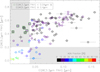 |
Fig. 2. Comparison between AKARI 3.3 μm PAH EQW and Spitzer/IRS 6.2 μm PAH EQW of the GOALS LIRG sample. The circles represent the sources with detections of both PAH features, whereas the left-pointing triangles represent detections of the 6.2 μm PAH but upper limits for the 3.3 μm PAH. The symbols are color-coded by the AGN bolometric fraction in the mid-infrared (Sect. 4.1; Díaz-Santos et al. 2017), which is indicated by the color bar shown in the bottom right. Galaxies with PAH3.3 μm EQW < 0.04 μm and PAH6.2 μm EQW ≥ 0.4 μm are also highlighted by the green squares. The gray regions are the areas where the implied galactic energy source (starburst or AGN) disagrees between 3.3 μm PAH EQW and 6.2 μm PAH EQW (high 3.3 μm PAH EQW but low 6.2 μm PAH EQW, or vice versa). |
In Fig. 3, we show the median AKARI + Spitzer spectra of galaxies with PAH6.2 μm EQW ≥ 0.4 μm, but with PAH3.3 μm EQW < 0.04 μm (green) or PAH3.3 μm EQW ≥ 0.04 μm (black). We made a cut of PAH6.2 μm EQW at a more strict value of 0.4 μm, instead of 0.2 μm, because we want to ensure a clean selection of starburst-dominated galaxies just by PAH6.2 μm EQW. We only use 6.2 μm PAH EQW to select starburst-dominated galaxies instead of the AGN fraction because the scope here is to compare the spectra of galaxies directly with their PAH EQWs. The AKARI continuum of the median spectrum with low PAH3.3 μm EQW is bluer, while the average Spitzer spectra are very similar. When the continua of the median AKARI spectra are fitted by a linear function avoiding the 3.05 μm (H2O ice) and 4.67 μm (CO ice and gas) absorption features, the slopes are −0.11 and −0.02 for sources with PAH3.3 μm EQW < 0.04 μm and PAH3.3 μm EQW ≥ 0.04 μm, respectively. It is also evident from these median spectra that sources with high 3.3 μm PAH EQW display a more prominent Brα emission.
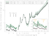 |
Fig. 3. Median spectra of sources with PAH6.2 μm EQW ≥ 0.4 μm, and PAH3.3 μm EQW < 0.04 μm (green; seven objects) or 3.3 μm PAH EQW ≥ 0.04 μm (black; 79 objects). The ranges of the spectra are 1σ uncertainties of the estimated median values. The inset panel shows a zoom-in of the 2.5–5 μm region with the continuum fits in red. The orange arrows indicate the wavelengths where the AKARI continuum color, Fν(4.3 μm)/Fν(2.8 μm), is measured. |
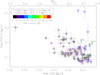 |
Fig. 4. Ratio of Brα to 3.3 μm PAH emission as a function of decreasing Brα EQW (increasing starburst age, the upper x-axis). The circles represent the sources with both 3.3 μm PAH and Brα detections color-coded by the AGN fraction. The upper limits are shown only for the objects with PAH3.3 μm EQW < 0.04 μm and PAH6.2 μm EQW ≥ 0.4 μm. The starburst ages are derived from the Brα EQW using the Starburst99 models (Leitherer et al. 1999, 2010; Vázquez & Leitherer 2005). |
4.2. Ionized gas in starburst-dominated LIRGs
Because the intensity of hydrogen recombination lines is directly related to the number of young, massive stars in star-forming regions, they provide an accurate estimate of the current star formation rate. Here we use the ratio of Brα4.05 μm/PAH3.3 μm to study the evolution of the ionization field in starburst-dominated GOALS LIRGs. In starburst-dominated galaxies, the Brα emission arises from HII regions ionized by young stars, while the continuum at 4 μm is dominated by emission from old stars. Thus, the Brα EQW measures the light-averaged ratio of the emission from young to old stars, and hence it can be used as an age indicator. Ages were estimated by generating a single burst of star formation using the Starburst99 evolutionary synthesis models (version; Leitherer et al. 1999, 2010; Vázquez & Leitherer 2005). We used a Kroupa initial mass function and the standard Geneva evolutionary tracks (0.5–10 Myr interval). The model output of Brγ EQW was converted to the Brα EQW, assuming Case B for hydrogen recombination, an effective temperature of ∼104 K, and a density3 of ∼100 cm−3. We also assume that there is just a single ionizing population of stars producing both the line and continuum emissions, which may not always be accurate, because in reality an underlying older stellar population from past star-forming episodes may also contribute to the near-infrared continuum. Hence, the ages derived from the Brα EQWs obtained with this simple model are upper limits to the true age of the current starburst.
In Fig. 4, we show the flux ratio of Brα to PAH3.3 μm as a function of Brα EQW. The range of Brα EQWs in the GOALS sample corresponds to ages of ∼5–10 Myr, with the majority of sources being between 6 and 7 Myr old. These ages are slightly higher than the ages of 1–4.5 Myr of the GOALS LIRGs estimated from the mid-infrared atomic fine-structure emission lines (Inami et al. 2013), but given that the Brα EQW ages are upper limits, they can be considered consistent. A clear correlation between Brα/PAH3.3 μm and Brα EQW is seen in starburst-dominated sources (with an AGN fraction less than 50%). The objects with PAH3.3 μm EQW < 0.04 μm and PAH6.2 μm EQW ≥ 0.4 μm (the green squares) are not detected in Brα. The AGN-dominated sources (AGN fraction >50%) do not follow the same trend: all of them have small Brα EQWs and their Brα/PAH3.3 μm ratios are between ∼0.1–0.25. We note that because an AGN can also contribute to the hydrogen recombination line emission, the estimated ages of the galaxies that have AGN present are probably not as reliable.
For starburst-dominated sources, the decrease of the Brα/PAH3.3 μm ratio with decreasing Brα EQW (increasing in starburst age) is consistent with the aging of the ionizing stellar populations, and thus with the reduction of Brα emission with stellar age. Our results are in agreement with the findings of Díaz-Santos et al. (2008, 2010) who show that in resolved star-forming regions of LIRGs, the ratio of the 11.3 μm PAH (and likely the 8.6 μm PAH) to Paα emission is correlated with the age of the HII regions as traced by Paα EQW. This trend simply reflects the different time-scales probed by the ionized gas and PAH emission, with the latter being also produced in more evolved stellar populations (a few tens of Myr) and not ascribed only to on-going star formation, because PAHs are excited by lower energy non-ionizing photons.
4.3. Contribution of PAH and Brα emission to LIR
Both PAH and Brα emission trace ongoing star formation and are often used to estimate SFRs. Here, we examine the ratio of the 3.3 μm PAH and Brα emission to the total infrared emission, which can also be used to estimate the SFR in LIRGs, free of the effects of extinction that can plague even the near-infrared emission. The 3.3 μm PAH and Brα emission used in this section were measured from the AKARI spectra that were extracted with the aperture covering ∼95% of the total flux in the AKARI 2D spectra (see Sect. 3). This aperture was also employed for the photometric measurements of the Spitzer Multiband Imaging Photometer (MIPS) imaging data. The MIPS data were used as follows, in order to estimate the infrared luminosity (LIR) inside this aperture. First, a fraction of the MIPS 24 μm flux density within this aperture and the flux density of the entire galaxy were measured. Then, this fraction was utilized as a scaling factor to convert LIR of the whole galaxy to LIR in the extraction aperture. Hereafter, we denote LIR 24 as the total infrared luminosity in this extraction aperture.
In the top panel of Fig. 5, we present the ratio of the 3.3 μm PAH luminosity to LIR 24 as a function of LIR 24. We show both the dust extinction uncorrected (small gray circles) and corrected (colored circles) PAH luminosities. The dust extinction is estimated based on the optical depth of the 9.7 μm silicate feature in the Spitzer/IRS spectra using Eq. (4) of Smith et al. (2007). The measurements of τ(9.7 μm) are taken from Stierwalt et al. (2014). The τ(9.7 μm) range of our sample is 0.46–8.38 with the mean and median of 1.92 and 1.57, respectively. There is a trend of decreasing L3.3 μm PAH/LIR 24 (a power-law function with an exponent of −0.55), indicating that an SFR based on uncorrected L3.3 μm PAH is likely to be underestimated for more infrared luminous galaxies. This trend has already been seen in the past for local LIRGs, which exhibit a deficit in L3.3 μm PAH/LIR (as well as in L6.2 μm PAH/LIR) compared with less infrared luminous galaxies (e.g., Kim et al. 2012; Yamada et al. 2013; Murata et al. 2017; Stierwalt et al. 2014). Although the extinction correction for PAH-based SFR calibrations is not common in the literature (e.g., Calzetti et al. 2007; Kennicutt et al. 2009; Shipley et al. 2016), when the dust extinction correction is applied, this trend becomes weaker, but it is still evident as a power-law function with an exponent of −0.24. All extreme outliers have PAH3.3 μm EQW < 0.04 μm.
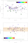 |
Fig. 5. Top: ratio of L3.3 μm PAH to LIR 24 as a function of LIR 24. The 3.3 μm PAH emission is measured from the AKARI spectra extracted with the aperture that covers ∼95% of the total flux in the AKARI 2D spectra. We use LIR 24 to denote the total infrared luminosity, scaled by the flux ratio of the Spitzer/MIPS 24 μm emission within the AKARI aperture to the total 24 μm flux (see Sect. 4.3 for more details). The sources with the detected emission feature are shown by the circles. The small gray circles denote the values without the dust extinction correction. The large circles are color-coded by the AGN fraction. The green squares represent the sources with PAH3.3 μm EQW < 0.04 μm and PAH 6.2 μm EQW ≥ 0.4 μm. Bottom: ratio of measured (gray) and corrected (colored) Brα to the infrared luminosity as a function of LIR 24. The horizontal orange solid line and shaded area indicate the mean and its standard deviation of the extinction corrected LBrα/LIR 24, respectively. The horizontal black dashed line indicates LBrα/LIR = 1.56 × 10⁻⁴ when the SFRs derived from LBrα and LIR 24 are the same. |
As shown in the bottom panel of Fig. 5, the mean and its standard deviation of the measured extinction corrected LBrα/LIR 24 are (1.55 ± 0.82) × 10−4, indicating that the SFR(LIR 24) and the extinction corrected SFR(Brα) are consistent (Kennicutt 1998). For the most infrared luminous galaxies, it is particularly important to perform the dust extinction correction based on the 9.7 μm absorption feature to bring the two measures in line across the sample (see also da Cunha et al. 2010).
5. Discussion
Based on our measurements of the combined AKARI and Spitzer spectra of 130 local LIRGs4, we examine the nature and properties of these galaxies from the GOALS sample. In this section, we propose an improved starburst/AGN diagnostic and explore ionization state and size distribution of the dust.
5.1. Nature of low 3.3 μ m PAH EQW starburst LIRGs
An empirical cut at PAH3.3 μm EQW < 0.04 μm has often been used to identify AGN-dominated sources (e.g., Moorwood 1986; Imanishi et al. 2010; Yamada et al. 2013). However, as we have shown in Sect. 4.1, out of 19 (or 24 including upper limits) sources with 3.3 μm PAH EQW in this range, ≳1/3 (7) have PAH6.2 μm EQW ≥ 0.4 μm, which implies that they are starburst-dominated galaxies. Based on the mid-infrared AGN diagnostics discussed in Sect. 4.1, none of these sources show any indication of AGN dominance even with the individual mid-infrared AGN indicators. Furthermore, close inspection of available archival optical spectra also indicates that they do not harbor an AGN. There is clearly a class of sources where the 3.3 μm PAH EQW alone can lead to erroneous identification of AGN, since it is very unlikely that the dust emission from an AGN dominates the 2–5 μm wavelength range but does not contribute significantly to the mid-infrared (T ∼ 500 K), given their intrinsically red, power-law continuum emission (Weedman et al. 2005; Armus et al. 2007). The following three factors may contribute to having a LIRG with a low EQW for 3.3 μm PAH (<0.04 μm) while the corresponding 6.2 μm PAH EQW remains >0.4 μm: (1) an absence of small PAH molecules, (2) a larger fraction of ionized PAH molecules, or (3) an excess of stellar emission at λ ≲ 5 μm. We discuss these hypotheses below.
Laboratory and numerical studies have shown that the relative strengths of the different PAH bands are expected to vary with the size and the ionization state of PAH molecules (Draine & Li 2001, 2007; Li & Draine 2001; Tielens 2008). This is caused by the different absorption cross section per C atom of neutral and ionized PAH (see Fig. 2 of Li & Draine 2001 and Fig. 3 of Draine & Li 2007). Ionization enhances the C-C stretching modes (6.2 and 7.7 μm) and the C–H in-plane bending mode (8.6 μm), but weakens the C–H stretching mode (3.3 μm) and the C–H out-of-plane bending mode (11.3 μm). In addition, PAH features for smaller grain sizes have emission peaks at shorter wavelengths. In other words, at a certain ionization state, when large dust grains are the predominant population, the 8.6 μm PAH feature shows stronger emission than the 6.2 μm PAH. Similarly, a harder ionization field produces a larger fraction of ionized PAH, such that the 3.3 μm PAH feature (and 11.3 μm PAH) is weaker, whereas the 6.2 μm PAH feature (as well as the 7.7 μm and 17 μm PAH features) is stronger. Thus, the PAH emission ratios such as PAH3.3 μm/PAH6.2 μm, PAH11.3 μm/PAH6.2 μm, and other combinations of ionized and neutral PAH emission can be used as indicators of the PAH ionization state. For example, Joblin et al. (1996) found that the PAH8.6 μm/PAH11.3 μm ratio depends on the relative populations of ionized and neutral PAH, which is supported by laboratory experiments (Hudgins & Allamandola 1995).
We use the flux ratio-ratio diagram of PAH11.3 μm/PAH7.7 μm and PAH6.2 μm/PAH7.7 μm as in Fig. 2 of Stierwalt et al. (2014) to investigate where the sources with low 3.3 μm and high 6.2 μm PAH EQWs lie compared with the entire sample. The PAH fluxes from the Spitzer data are also taken from Stierwalt et al. (2014). The sources with the low 3.3 μm and high 6.2 μm PAH EQWs (i.e., the squares in Fig. 2) are distributed over a wide range of the grain size and ionization state without any obviously biased distributions compared to the other sources. In addition, these sources do not show particularly weak 3.3 μm PAH emission relative to 6.2 μm PAH emission. A direct flux comparison of the 3.3 μm and 6.2 μm PAH features of these sources is consistent with the distribution of the rest of our sample, except for IC 0860 whose F6.2PAH/F3.3PAH ratio is about a factor of five higher than the average of the entire sample. Therefore, the fact that they (possibly except IC 0860) have low 3.3 μm and high 6.2 μm PAH EQWs is related to the continuum properties, not the PAH properties.
Next, we examine the 6.2 μm PAH EQW versus the 2–5 μm continuum in Fig. 6. With one exception, all LIRGs with AKARI flux density ratios Fν(4.3 μm)/Fν(2.8 μm) ≲ 1 display PAH6.2 μm EQW > 0.2 μm. When only LIRGs with PAH6.2 μm EQW < 0.4 μm are considered, sources with lower PAH EQWs tend to show progressively redder continuum slopes. More strikingly, galaxies for which there is inconsistency between the 3.3 μm and 6.2 μm PAH EQW starburst/AGN classifications (i.e., those with PAH6.2 μm EQW ≥ 0.4 μm and PAH3.3 μm EQW < 0.04 μm, the circles with the green square) occupy the same region as those for which both diagnostics indicate that they are dominated by star formation. That is, they have 2–5 μm continuum slopes as blue as or bluer (Fν(4.3 μm)/Fν(2.8 μm) ≲ 0.9) than most of the pure star-forming LIRGs. The bluer slope can also be identified in Fig. 3.
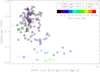 |
Fig. 6. PAH6.2 μm EQW plotted against the AKARI 2.5–5 μm continuum slope as measured by the Fν(4.3 μm)/Fν(2.8 μm) ratio (see also Fig. 3). The symbols are the same as in Fig. 2. |
Therefore, the 2–5 μm continua in some of the LIRGs with the lowest 3.3 μm PAH EQWs are not necessarily dominated by hot dust emitted by the optically thick dusty torus of a putative central AGN. To explore this further, in Fig. 7 we plot the ratio of K-band, a first order tracer of stellar mass of the entire galaxy, to 5 μm monochromatic emission, as a function of the 3.3 μm PAH EQW to probe the dominant source of the continuum emission. Galaxies with PAH3.3 μm EQW < 0.04 μm roughly split into two different populations depending on their K-band/5 μm ratios. Among these galaxies, interestingly, when their 6.2 μm PAH EQWs are high (≥0.4 μm, green squares), they also show higher K-band/5 μm ratios (≳ 1.0). On the other hand, the galaxies with PAH6.2 μm EQW < 0.2 μm (red diamonds) have K-band/5 μm ≲ 1.0. The higher K-band/5 μm ratio for the galaxies with the low 3.3 μm PAH and high 6.2 μm PAH EQWs indicates a larger stellar contribution at K-band, which is likely produced by the stellar continuum of more massive, evolved stars rather than hot dust.
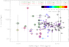 |
Fig. 7. Ratio of 2MASS K-band to 5 μm monochromatic continuum emission as a function of 3.3 μm PAH EQW. The EQWs are derived from the AKARI spectra extracted with an aperture covering ∼95% of the total AKARI flux. The K-band emission is measured in the imaging data using the same aperture size. The symbols are the same as in Fig. 2, in addition to the red diamonds, which indicate PAH3.3 μm EQW < 0.04 μm and PAH6.2 μm EQW < 0.4 μm. |
Dust extinction cannot cause the discrepancy between the PAH EQW3.3 μm and EQW 6.2 μm diagnostics, because it would also suppress the 3.3 μm PAH flux with respect to the 6.2 PAH flux. However, if the ∼3 μm continuum is dominated by stellar emission instead of hot dust and the ∼3 μm continuum emission is more extended than the 3.3 μm PAH flux, this may decrease the PAH EQW3.3 μm with respect to the PAH EQW6.2 μm. Because the IRS slit is narrow, we inspect these galaxies to check whether they are more distant, such that more emission from galaxy disks is covered by the slit. We find that their luminosity distances are around the median distance of the entire sample, except ESO 077-IG014 which is at 186 Mpc. Therefore, while stellar emission could be the source of the decreased 3.3 μm PAH EQW, a greater distance is not responsible for the excess disk emission in these sources.
These analyses suggest that stellar emission plays an important role in some LIRGs. While these galaxies are actively star-forming, there is very little hot dust contributing to their observed 3 μm emission. This hot dust could be highly compact and obscured, or these galaxies may simply have less hot dust because of a more distributed or aging nuclear burst.
5.2. Further constraints on the AKARI starburst/AGN diagnostics
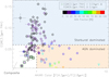 |
Fig. 8. Revised starburst/AGN diagnostic diagram using 3.3 μm PAH EQW and Fν(4.3 μm)/Fν(2.8 μm). The symbols are the same as in Fig. 2. The blue and beige areas are the regions we propose for identifying LIRGs whose infrared continuum emission is dominated by starbursts or AGN, respectively (see also Eqs. (1) and (2)). The white area denotes composite sources (Eq. (3)). |
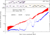 |
Fig. 9. Top: JWST filter response curves. The purple and orange curves denote the NIRCam and MIRI filters, respectively. Bottom: median SEDs of starburst- (blue) and AGN-dominated (red) LIRGs. The starburst- and AGN-dominated galaxies are selected to have the AGN fractions <30% and ≥60%, respectively. The SEDs are shown in the rest-frame. The median fluxes are manually scaled to avoid any overlap between the SEDs. The 1.2–2.2 μm, 2.5–5 μm, and 5–38 μm data are from 2MASS, AKARI, and Spitzer, respectively. The redshifted SEDs (z = 0.3–5.0) are shown in Fig. A.1. The SEDs are available as online data at the CDS. |
Several studies have proposed using the 3.3 μm PAH EQW or the 2–5 μm continuum slope (Γ; Fν ∝ λΓ) from AKARI as diagnostics for the identification of obscured AGN in LIRGs (Imanishi et al. 2010; Lee et al. 2012). The parameter space within which galaxies harboring an AGN are found, is normally assumed to have PAH3.3 μm EQW < 0.04 μm or Γ(Fλ ∝ λΓ) > −1 (equivalent to Γ(Fν ∝ λΓ) > 1, Risaliti et al. 2010; Sani et al. 2008; Imanishi et al. 2010). However, these studies are limited to the information available at 2–5 μm, which is where the hottest dust emission from the obscured AGN (T > 1000 K) and direct photospheric starlight are in competition with each other.
The mid-infrared is a much cleaner wavelength regime in which to search for buried AGN (Laurent et al. 2000; Sturm et al. 2002; Armus et al. 2007; Desai et al. 2007; Petric et al. 2011; Alonso-Herrero et al. 2012). This is where warm (T ∼ 300–500 K) dust from the torus can contribute significantly to the continuum emission (Desai et al. 2007; Spoon et al. 2007; Petric et al. 2011; Díaz-Santos et al. 2011).
Based on the additional information provided by the Spitzer/IRS data, we propose a revision of the commonly used starburst/AGN diagnostic in the 2–5 μm range. This involves the 3.3 μm PAH EQW and the continuum slope, Γ, which we trace using the flux density ratio, Fν(4.3 μm)/Fν(2.8 μm). We prefer the flux ratio because Γ requires fitting the continuum slope, and a wide variation in the slope within the 2–5 μm range (Fig. B.1) can easily cause unreasonable fits (and corresponding Γ values).
We propose revised boundaries between starburst- and AGN-dominated galaxies as follows:


We display this new diagnostic for the GOALS AKARI sample in Fig. 8. In most cases, the 3.3 μm PAH EQW can be used to select starburst-dominated galaxies. While many other studies have drawn similar limits on these measurements to derive near-infrared diagnostics for AGN searches, they use these two limits (the PAH EQW and color) independently. We require instead that both quantities be taken into account. Otherwise as much as 1/3 of our LIRG sample with PAH3.3 μm EQW < 0.04 μm could be misclassified as AGN when they are more likely to be starburst-dominated galaxies.
Sources in which both star formation and AGN may contribute significantly to the near- and mid-infrared emission are:
We cannot completely rule out the possibility that LIRGs that meet the conditions of Eq. (3) are AGN. Nevertheless, as shown in Sect. 5.1, at least the near and mid-infrared emission of these LIRGs is likely dominated by star formation processes, which implies that AGN probably do not contribute significantly to the bolometric luminosity of these galaxies. In fact, their AGN fractions are ≲50%.
5.3. Applications to JWST observations
With the 2.5–38 μm spectra of a large sample of local LIRGs, we are able to investigate the effectiveness of using the existing JWST/NIRCam and JWST/MIRI filters to select starburst and AGN. In order to fully cover the JWST wavelength range, we have also measured the J, H, and KS-band fluxes using the imaging data from the Two Micron All Sky Survey (2MASS, Skrutskie et al. 2006). The centroid of the photometry aperture is the same as the Spitzer pointing, which is also the spectral extraction position of the AKARI data. The aperture size is 10.5″ to match the AKARI and Spitzer spectral extractions (see Sect. 3). The median SEDs of starburst and AGN-dominated LIRGs from our sample are shown in Fig. 9, along with the JWST filter response curves for reference. To create these median spectra, we combine all LIRGs with AGN fractions less than 30% as starburst-dominated, and all those with AGN fractions more than 60% as AGN-dominated. In the following subsections, the 1.2–38 μm SEDs of individual galaxies and the median SEDs of the starburst- and AGN-dominated galaxies shown in Fig. 9 are employed to explore AGN color selections and 3.3 μm PAH spectro-photometry using the JWST photometric filters.
5.3.1. AGN color selections
In Fig. 10, we show a color-color diagram of the JWST filters F770W/F444W versus F560W/F356W. These broadband filters are selected to be closest to the color combinations of the Spitzer/IRAC filters for the AGN selection in Lacy et al. (2004) and Donley et al. (2012). We adapt the same IRAC color boundaries for our JWST color-color diagram. Donley et al. (2012) have explored the color evolution of galaxies with various AGN contributions using the redshifted SED templates of Polletta et al. (2008) and Dale & Helou (2002) in the IRAC color-color diagram. Here we artificially redshift our combined 2MASS, AKARI, and Spitzer SEDs from z = 0 to z = 1.5 in steps of Δz = 0.3 to explore their color evolution in the JWST color-color diagram.
As shown in Fig. 10, AGN-dominated galaxies are mostly found within the AGN selection boundaries of both Lacy et al. (2004) and Donley et al. (2012) up to z = 1.5, while starburst-dominated galaxies become bluer in both of the colors from z = 0 to 0.3. At higher redshifts, starburst-dominated galaxies enter and remain within the AGN boundaries of Lacy et al. (2004) and cannot be separated from the AGN-dominated galaxies. On the other hand, the boundaries of Donley et al. (2012) give a cleaner selection as expected. This trend agrees well with the results of Donley et al. (2012) that pure starburst galaxies at 0.5 < z < 1.5 become bluer and lie on the bottom left side just outside of the AGN selection boundaries. For this color-color selection, we can only perform the test up to z = 1.5 because of the wavelength coverage of our SEDs, whose blue end (2MASS J-band) shifts out from the coverage of F356W.
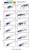 |
Fig. 10. AGN infrared color selection with the JWST filters adopted from Lacy et al. (2004; dotted line) and (Donley et al. 2012; solid line). The circles indicate individual LIRGs with the color coding of the AGN fraction shown at the top of the figure. The blue (starburst) and red (AGN) stars indicate the median SEDs from Fig. 9. The panels show the changes of the galaxy colors with the redshift varying from the top (z = 0.0) to the bottom (z = 1.5) in steps of Δz = 0.3. The left column shows the full range of the galaxy color distribution, while the right column shows a magnified portion of the left plot. The plots are shown only up to z = 1.5 due to the wavelength limit (2MASS J-band) of our SEDs being shifted beyond the coverage of F356W. |
In addition to adapting the IRAC color selections, we also explore other possible color selection criteria based entirely on the JWST filters. The best approach would be to use the NIRCam medium-band filters to isolate the 3.3 μm PAH EQW using the F335M/F300M flux ratio and detect hot dust emission using F430M/F250M for galaxies at z ∼ 0.4. However, the red wavelength limit of the medium-band filters at F480M prevents us from applying this method for galaxies at higher redshifts (z ≥ 0.4). We have tried the same experiment using the broadband filters (e.g., F356W/F277W vs. F444W/F200W for z = 0) in order to apply the same selection method to higher redshifts. However, this does not provide a clean separation between AGN- and starburst-dominated sources, due to the intrinsically low PAH EQW.
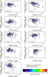 |
Fig. 11. AGN/starburst diagnostic diagrams at each of the redshifts indicated at the bottom left of each panel. The y-axis represents 3.3 μm PAH EQW by taking the flux ratio of the filter covering the 3.3 μm PAH feature to the estimated local continuum emission via a linear interpolation between the two bracketing filters. The x-axis is a measure of hot dust emission. The symbols are the same as in Fig. 10. The vertical dotted line at the colors of 1.5 in each panel indicates an empirical cut for selecting starburst-dominated galaxies. |
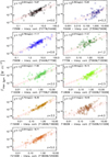 |
Fig. 12. PAH3.3 um fluxes obtained in AKARI spectra compared with an estimate of the 3.3 μm PAH fluxes using three JWST broadband filters from z = 0 to 5.0. At z = 0, the 3.3 μm PAH fluxes are the actual measurements from the AKARI spectra, while for higher redshifts, they are manually scaled to the expected 3.3 μm PAH fluxes of high-z ULIRGs (see text for more details). The broadband estimated PAH fluxes are indicated by the difference between the spectro-photometry in the filter covering the 3.3 μm PAH feature and its local continuum calculated by the linear interpolation of its two neighboring filters. The red solid and dashed lines indicate the best fit line (shown at the top left in each panel) and its 1σ uncertainty, respectively. |
Instead of using a simple color to represent the PAH EQW, we assume that the local continuum of the 3.3 μm PAH feature is the linear interpolation of the two filters that bracket the filter covering the 3.3 μm PAH feature to give an estimate of 3.3 μm PAH EQW (e.g., at z = 0, the PAH is in F336W, and F277W and F444W are used to compute its local continuum). In Fig. 11, the ratio of the flux in the filter band of the PAH feature to the estimated local continuum is used to approximate the 3.3 μm PAH EQW (y-axis). This represents a reproduction of Fig. 8 using the JWST filters. The flux ratio along the x-axis indicates the continuum slope, which traces the strength of hot dust emission. Due to relatively low 3.3 μm emission compared to the broadband filters, it can be challenging to accurately estimate actual EQW values, but the hot dust indicator still works well to identify dust-embedded AGN.
For galaxies with a rest-frame 2–5 μm color (x-axis) of <1.5, all of them are starburst-dominated (with AGN fraction less than 50%). All of the AGN-dominated sources have a color of >1.5, as do some of the starbursts. Among all of the starburst sources, about 20–30% (except at z = 0.3, which is 45%) have colors of ≥1.5. While selections of AGN-dominated sources with colors at ≥1.5 at each redshift include some contaminants, the color limit of ≲1.5 can act as a reasonable empirical limit for selecting starburst-dominated galaxies up to z = 5.
Best fit linear coefficients relating 3.3 μm PAH flux to JWST filter color excess from z = 0.0 to z = 5.0.
5.3.2. PAH flux inferred from JWST broadband photometry
Here we examine whether we can use the JWST broadband filters to estimate the 3.3 μm PAH flux by identifying a color excess. Using our sample, we estimate the flux of the 3.3 μm PAH emission assuming L3.3μm PAH/LIR ∼ 0.1% (Fig. 5 top). For a system with LIR = 1012 L⊙, the expected 3.3 μm PAH fluxes are 3.2 × 10⁻¹⁵ W m−2 at z ∼ 0, 4.6 × 10⁻¹⁹ W m−2 at z ∼ 1.2, and 1.4 × 10⁻²⁰ W m−2 at z ∼5. Based on the unresolved line sensitivity of JWST/MIRI spectroscopy (Glasse et al. 2015), this suggests that the feature would be detectable out to z ∼ 4.5 at 10σ within 10 000 s of on-source exposure time.
Following the methodology described in the previous section, we assume a linear interpolation of two neighboring filters to represent the local continuum under the 3.3 μm PAH feature. An advantage of using 3.3 μm PAH is that the local continuum is often flatter than the other PAH features and rarely has strong absorption or emission features around 3.3 μm to interfere with measuring the excess in a broadband filter. In addition, although the 3.3 μm PAH EQW is on average about a factor of ten smaller than 6.2 μm PAH EQW, it is the only PAH feature that can be observed with JWST at z > 3.5.
In Fig. 12, we show the 3.3 μm PAH flux as measured with our AKARI spectra against the 3.3 μm color excess. At z = 0, the PAH fluxes are the actual measurements from our spectra, but for higher redshifts, at each redshift we arbitrarily scale all of the 3.3 μm PAH fluxes with a single scaling factor to the expected values for high-z ULIRGs (≳1012 L⊙). As discussed above, the expected fluxes are calculated assuming that the 3.3 μm PAH emission on average contributes about 0.1% to the total infrared emission. At z = 0, F336W covers the PAH feature, and F277W and F444W are used to estimate its local continuum. The spectro-photometrically estimated 3.3 μm excesses correlate quite well with the directly measured 3.3 μm PAH fluxes in the AKARI spectra. This suggests that we are able to infer 3.3 μm PAH fluxes based on the JWST broadband photometry for most LIRGs. The dispersion along the x-axis is likely caused by the PAH sub-peak, H2O ice absorption, and CO absorption features in the AKARI spectral range. If these are indeed the reasons, this dispersion is real, and is a fundamental limit to estimating the 3.3 μm PAH flux via photometry. Among the redshift bins in Fig. 12, the dispersion around the regression fit is smallest at z = 3.5 and z = 0.6, which provides the most reliable estimate of 3.3 μm PAH fluxes. There are more substantial outliers seen at redshifts of 1.2, 2.5, and 4.0. At z = 1.2, the 3.3 μm PAH feature is covered by F770W, which has λ/Δλ = 3.5, the smallest among the MIRI filters. This may cause a larger uncertainty when estimating 3.3 μm PAH fluxes. At z = 2.5, the PAH falls at the blue edge of F1280W and it is only partially covered by the filter. At z = 4.0, the PAH is in both F1800W and F1500W, which may cause a larger scatter. Although the dispersions are larger in some redshift bins, this correlation holds up to z = 5, to the reddest JWST coverage. We summarize the coefficients for the correlation, F3.3 PAH = 10a⋅log(Excess) + b, at each redshift in Table 2. At z = 3.5, which shows the tightest correlation, the photometric excess of 1 corresponds to  , while in the redshift bin z = 1.2, which has one of the largest dispersions, the estimated flux has a larger uncertainty,
  . With the excess calculated using three JWST broadband filters, these relations offer an estimate of 3.3 μm PAH fluxes, which, in particular, could be useful for identifying strong sources of PAH emission (starbursts) in high-redshift groups or clusters (e.g., Duc et al. 2002; Saintonge et al. 2008; Koyama et al. 2008).
6. Summary and conclusions
We present analyses of 145 local LIRGs of the GOALS galaxy sample with available AKARI spectra, covering the 2.5–5 μm rest-frame wavelength. We combine the measurements taken from the AKARI spectra, such as the 3.3 μm PAH feature, the Brα emission line, and the 2.5–5 μm continuum slope, with mid-infrared measurements obtained from Spitzer spectra, such as the 6.2 μm PAH feature, to study the nature of the local LIRG population. Based on our findings, we also explore potential starburst/AGN diagnostics in the JWST era. We have obtained the following results:
The relation between the 3.3 μm and 6.2 μm PAH EQWs shows that starburst-dominated galaxies, identified by 6.2 μm PAH EQW ≥ 0.6 μm, cover a wide range of the 3.3 μm PAH EQW from 0.05 μm to 0.16 μm. Despite the large spread in the 3.3 μm PAH EQW compared with the 6.2 μm PAH EQW, the 3.3 μm PAH EQW is an effective diagnostic for selecting starburst-dominated galaxies in most cases.
We find that a significant fraction (≳1/3) of the galaxies with PAH3.3 μm EQW < 0.04 μm, which would typically be considered as AGN-dominated sources, have high 6.2 μm PAH EQWs (≥0.4 μm), suggesting that they are instead starburst-dominated. These galaxies have AKARI continua as blue as those showing high EQWs in both 3.3 μm and 6.2 μm PAH features. While the median Spitzer spectra of these two types of sources are remarkably similar, their median AKARI spectra are significantly different. We suggest that they are in fact galaxies whose 2–5 μm continua are dominated by strong stellar emission rather than hot dust, which also reduces the 3.3 μm PAH EQW to very low levels. For this class of galaxy, measuring the near- to mid-infrared continuum slope is critical to properly assess the dominant power source. The use of the 3.3 μm PAH EQW alone is not adequate to select AGN-dominated galaxies in all cases.
We exploit the 6.2 μm PAH EQW as well as our estimated bolometric AGN contribution provided by the Spitzer/IRS spectra to propose a revised starburst/AGN diagnostic diagram based on 2.5–5 μm spectroscopic data. We use the 3.3 μm PAH EQW and the 2.5–5 μm continuum slope, as measured by the Fν(4.3 μm)/Fν(2.8 μm) flux ratio, to establish that starburst-dominated sources have PAH3.3 μm EQW ≥ 0.06 μm, while AGN-dominated sources have both PAH3.3 μm EQW < 0.06 μm and Fν(4.3 μm)/Fν(2.8 μm) ≥ 1.0.
A clear correlation is seen between LBrα and LIR regardless of the galactic energy source when the dust extinction correction is applied using the 9.7 μm silicate absorption. The SFRs estimated from the extinction corrected Brα agree well with SFRs estimated from the total infrared luminosity.
Based on the combined 2MASS, AKARI, and Spitzer data for the individual galaxies, we have explored starburst/AGN diagnostics with the JWST filters. Commonly used Spitzer/IRAC color selection diagrams of Lacy et al. (2004) and Donley et al. (2012) are adapted for the JWST filters. While they perform well up to z ∼ 0.3, at higher redshifts, starburst-dominated galaxies start to contaminate the AGN selection of Lacy et al. (2004), while the boundaries of Donley et al. (2012) work well at least up to z = 1.5.
Although a clean selection of AGN-dominated sources is difficult, one of the simplest starburst selections that can be used up to z ∼ 5 with JWST is to measure the rest-frame 2–5 μm continuum slope using the broadband filters to exclude galaxies with hot dust emission. The rest-frame 2–5 μm continuum color cut at <1.5 (e.g., F1280W/F560 for z ∼ 2.0) successfully retrieves 70–80% of the starburst-dominated galaxies.
Artificially redshifting the combined 2MASS, AKARI, and Spitzer spectra from z = 0 to 5, we measure the excess of 3.3 μm PAH emission in a JWST filter using its neighboring filters to remove the local continuum. This excess correlates well with the 3.3 μm PAH fluxes measured directly in the AKARI spectra up to z = 5. In particular, we find that the most reliable estimate is at z = 3.5 and z = 0.6. This correlation can be useful for identifying obscured star formation in high-z galaxies with JWST photometry.
Available at http://www.ir.isas.jaxa.jp/AKARI/Observation/support/IRC/
The median electron density of the entire GOALS sample is ∼300 cm−3, estimated with the [S III] mid-infrared emission line ratios (Inami et al. 2013).
There are 15 sources that are not included in the direct comparisons between their AKARI and Spitzer data because of mismatched pointings or their extended morphologies (Sect. 4).
Acknowledgments
The authors would like to thank the referee whose constructive comments helped to improve the manuscript. We would also like to thank the language editor Ruth Chester at A&A for helpful revisions of this manuscript. HI appreciate Grant-in-Aid for Japan Society for the Promotion of Science (JSPS) Fellows (21-969) and JSPS Excellent Young Researchers Overseas Visit Program for supporting this work at the Spitzer Science Center, California Institute of Technology, USA. YO acknowledges support from Ministry of Science and Technology (MOST) of Taiwan 106-2112-M-001-008-. This research is based on observations with AKARI, a JAXA project with the participation of ESA. The authors appreciated the opportunity to present this work at the 4th AKARI international conference, which helped to enrich this work (Inami et al. 2018). The Spitzer Space Telescope is operated by the Jet Propulsion Laboratory, California Institute of Technology, under NASA contract 1407. This research has made use of the NASA/IPAC Extragalactic Database (NED) and the Infrared Science Archive (IRSA), which are operated by the Jet Propulsion Laboratory, California Institute of Technology, under contract with the National Aeronautics and Space Administration.
References
- Alonso-Herrero, A., Pereira-Santaella, M., Rieke, G. H., & Rigopoulou, D. 2012, ApJ, 744, 2 [NASA ADS] [CrossRef] [Google Scholar]
- Armus, L., Charmandaris, V., Bernard-Salas, J., et al. 2007, ApJ, 656, 148 [NASA ADS] [CrossRef] [Google Scholar]
- Armus, L., Mazzarella, J. M., Evans, A. S., et al. 2009, PASP, 121, 559 [Google Scholar]
- Brandl, B. R., Bernard-Salas, J., Spoon, H. W. W., et al. 2006, ApJ, 653, 1129 [NASA ADS] [CrossRef] [Google Scholar]
- Calzetti, D., Kennicutt, R. C., Engelbracht, C. W., et al. 2007, ApJ, 666, 870 [NASA ADS] [CrossRef] [Google Scholar]
- da Cunha, E., Charmandaris, V., Díaz-Santos, T., et al. 2010, A&A, 523, A78 [NASA ADS] [CrossRef] [EDP Sciences] [Google Scholar]
- Dale, D. A., & Helou, G. 2002, ApJ, 576, 159 [NASA ADS] [CrossRef] [Google Scholar]
- Desai, V., Armus, L., Spoon, H. W. W., et al. 2007, ApJ, 669, 810 [NASA ADS] [CrossRef] [Google Scholar]
- Díaz-Santos, T., Alonso-Herrero, A., Colina, L., et al. 2008, ApJ, 685, 211 [NASA ADS] [CrossRef] [Google Scholar]
- Díaz-Santos, T., Alonso-Herrero, A., Colina, L., et al. 2010, ApJ, 711, 328 [NASA ADS] [CrossRef] [Google Scholar]
- Díaz-Santos, T., Charmandaris, V., Armus, L., et al. 2011, ApJ, 741, 32 [NASA ADS] [CrossRef] [Google Scholar]
- Díaz-Santos, T., Armus, L., Charmandaris, V., et al. 2017, ApJ, 846, 32 [Google Scholar]
- Doi, Y., Takita, S., Ootsubo, T., et al. 2015, PASJ, 67, 50 [NASA ADS] [Google Scholar]
- Donley, J. L., Koekemoer, A. M., Brusa, M., et al. 2012, ApJ, 748, 142 [NASA ADS] [CrossRef] [Google Scholar]
- Draine, B. T., & Li, A. 2001, ApJ, 551, 807 [NASA ADS] [CrossRef] [Google Scholar]
- Draine, B. T., & Li, A. 2007, ApJ, 657, 810 [NASA ADS] [CrossRef] [Google Scholar]
- Duc, P.-A., Poggianti, B. M., Fadda, D., et al. 2002, A&A, 382, 60 [NASA ADS] [CrossRef] [EDP Sciences] [Google Scholar]
- Gallimore, J. F., Yzaguirre, A., Jakoboski, J., et al. 2010, ApJS, 187, 172 [NASA ADS] [CrossRef] [Google Scholar]
- Genzel, R., & Cesarsky, C. J. 2000, ARA&A, 38, 761 [NASA ADS] [CrossRef] [Google Scholar]
- Glasse, A., Rieke, G. H., Bauwens, E., et al. 2015, PASP, 127, 686 [NASA ADS] [CrossRef] [Google Scholar]
- Haan, S., Armus, L., Laine, S., et al. 2011, ApJS, 197, 27 [NASA ADS] [CrossRef] [Google Scholar]
- Houck, J. R., Roellig, T. L., van Cleve, J., et al. 2004, ApJS, 154, 18 [NASA ADS] [CrossRef] [Google Scholar]
- Howell, J. H., Armus, L., Mazzarella, J. M., et al. 2010, ApJ, 715, 572 [Google Scholar]
- Hudgins, D. M., & Allamandola, L. J. 1995, J. Phys. Chem., 99, 3033 [CrossRef] [PubMed] [Google Scholar]
- Imanishi, M., Nakagawa, T., Ohyama, Y., et al. 2008, PASJ, 60, 489 [Google Scholar]
- Imanishi, M., Nakagawa, T., Shirahata, M., Ohyama, Y., & Onaka, T. 2010, ApJ, 721, 1233 [NASA ADS] [CrossRef] [Google Scholar]
- Inami, H., Armus, L., Charmandaris, V., et al. 2013, ApJ, 777, 156 [NASA ADS] [CrossRef] [Google Scholar]
- Inami, H., Matsuhara, H., Armus, L., et al. 2018, JAXA-SP-17-009E, 221 [Google Scholar]
- Ishihara, D., Onaka, T., Kataza, H., et al. 2010, A&A, 514, A1 [NASA ADS] [CrossRef] [EDP Sciences] [Google Scholar]
- Joblin, C., Tielens, A. G. G. M., Geballe, T. R., & Wooden, D. H. 1996, ApJ, 460, L119 [NASA ADS] [CrossRef] [Google Scholar]
- Kennicutt, Jr., R. C. 1998, ApJ, 498, 541 [NASA ADS] [CrossRef] [Google Scholar]
- Kennicutt, Jr., R. C. Hao, C.-N., Calzetti, D., et al. 2009, ApJ, 703, 1672 [NASA ADS] [CrossRef] [Google Scholar]
- Kim, J. H., Im, M., Lee, H. M., et al. 2012, ApJ, 760, 120 [NASA ADS] [CrossRef] [Google Scholar]
- Koyama, Y., Kodama, T., Shimasaku, K., et al. 2008, MNRAS, 391, 1758 [NASA ADS] [CrossRef] [Google Scholar]
- Lacy, M., Storrie-Lombardi, L. J., Sajina, A., et al. 2004, ApJS, 154, 166 [NASA ADS] [CrossRef] [Google Scholar]
- Laurent, O., Mirabel, I. F., Charmandaris, V., et al. 2000, A&A, 359, 887 [NASA ADS] [Google Scholar]
- Lee, J. C., Hwang, H. S., Lee, M. G., Kim, M., & Lee, J. H. 2012, ApJ, 756, 95 [NASA ADS] [CrossRef] [Google Scholar]
- Leitherer, C., Schaerer, D., Goldader, J. D., et al. 1999, ApJS, 123, 3 [Google Scholar]
- Leitherer, C., Ortiz Otálvaro, P. A., Bresolin, F., et al. 2010, ApJS, 189, 309 [NASA ADS] [CrossRef] [Google Scholar]
- Li, A., & Draine, B. T. 2001, ApJ, 554, 778 [Google Scholar]
- Madau, P., & Dickinson, M. 2014, ARA&A, 52, 415 [NASA ADS] [CrossRef] [Google Scholar]
- Moorwood, A. F. M. 1986, A&A, 166, 4 [NASA ADS] [Google Scholar]
- Murakami, H., Baba, H., Barthel, P., et al. 2007, PASJ, 59, 369 [Google Scholar]
- Murata, K., Nakagawa, T., Matsuhara, H., & Yano, K. 2017, PASJ, submitted [ArXiv: 1707.01652] [Google Scholar]
- Ohyama, Y., Onaka, T., Matsuhara, H., et al. 2007, PASJ, 59, 411 [NASA ADS] [Google Scholar]
- Onaka, T., Matsuhara, H., Wada, T., et al. 2007, PASJ, 59, 401 [NASA ADS] [Google Scholar]
- Peeters, E., Spoon, H. W. W., & Tielens, A. G. G. M. 2004, ApJ, 613, 986 [NASA ADS] [CrossRef] [Google Scholar]
- Petric, A. O., Armus, L., Howell, J., et al. 2011, ApJ, 730, 28 [NASA ADS] [CrossRef] [Google Scholar]
- Polletta, M., Weedman, D., Hönig, S., et al. 2008, ApJ, 675, 960 [NASA ADS] [CrossRef] [Google Scholar]
- Risaliti, G., Imanishi, M., & Sani, E. 2010, MNRAS, 401, 197 [NASA ADS] [CrossRef] [Google Scholar]
- Saintonge, A., Tran, K.-V. H., & Holden, B. P. 2008, ApJ, 685, L113 [NASA ADS] [CrossRef] [Google Scholar]
- Sanders, D. B., Mazzarella, J. M., Kim, D.-C., Surace, J. A., & Soifer, B. T. 2003, AJ, 126, 1607 [Google Scholar]
- Sani, E., Risaliti, G., Salvati, M., et al. 2008, ApJ, 675, 96 [NASA ADS] [CrossRef] [Google Scholar]
- Shipley, H. V., Papovich, C., Rieke, G. H., Brown, M. J. I., & Moustakas, J. 2016, ApJ, 818, 60 [NASA ADS] [CrossRef] [Google Scholar]
- Skrutskie, M. F., Cutri, R. M., Stiening, R., et al. 2006, AJ, 131, 1163 [NASA ADS] [CrossRef] [Google Scholar]
- Smith, J. D. T., Draine, B. T., Dale, D. A., et al. 2007, ApJ, 656, 770 [NASA ADS] [CrossRef] [Google Scholar]
- Spoon, H. W. W., Marshall, J. A., Houck, J. R., et al. 2007, ApJ, 654, L49 [NASA ADS] [CrossRef] [Google Scholar]
- Stierwalt, S., Armus, L., Surace, J. A., et al. 2013, ApJS, 206, 1 [NASA ADS] [CrossRef] [Google Scholar]
- Stierwalt, S., Armus, L., Charmandaris, V., et al. 2014, ApJ, 790, 124 [NASA ADS] [CrossRef] [Google Scholar]
- Sturm, E., Lutz, D., Tran, D., et al. 2000, A&A, 358, 481 [NASA ADS] [Google Scholar]
- Sturm, E., Lutz, D., Verma, A., et al. 2002, A&A, 393, 821 [NASA ADS] [CrossRef] [EDP Sciences] [Google Scholar]
- Takita, S., Doi, Y., Ootsubo, T., et al. 2015, PASJ, 67, 51 [NASA ADS] [CrossRef] [Google Scholar]
- Tielens, A. G. G. M. 2008, ARA&A, 46, 289 [NASA ADS] [CrossRef] [EDP Sciences] [Google Scholar]
- Tokunaga, A. T., Sellgren, K., Smith, R. G., et al. 1991, ApJ, 380, 452 [NASA ADS] [CrossRef] [Google Scholar]
- Vázquez, G. A., & Leitherer, C. 2005, ApJ, 621, 695 [NASA ADS] [CrossRef] [Google Scholar]
- Weedman, D. W., Hao, L., Higdon, S. J. U., et al. 2005, ApJ, 633, 706 [NASA ADS] [CrossRef] [Google Scholar]
- Woo, J.-H., Kim, J. H., Imanishi, M., & Park, D. 2012, AJ, 143, 49 [NASA ADS] [CrossRef] [Google Scholar]
- Yamada, R., Oyabu, S., Kaneda, H., et al. 2013, PASJ, 65, 103 [NASA ADS] [Google Scholar]
- Yano, K., Nakagawa, T., Isobe, N., & Shirahata, M. 2016, ApJ, 833, 272 [NASA ADS] [CrossRef] [Google Scholar]
Appendix A: The redshifted median SEDs of starburst- and AGN-dominated sources
In Fig. A.1, we show the redshifted median SEDs of starburst- and AGN-dominated sources, which are presented in Fig. 9. The redshift bins match the ones used in Figs. 11 and 12.
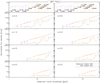 |
Fig. A.1. Same plots as Fig. 9, but the SEDs are redshifted from z = 0.3 to 5.0 as indicated in each panel. The orange circles on each SED indicate the locations of the effective wavelengths of the JWST filters shown in the upper most panels. |
Appendix B: The AKARI spectra
All of the AKARI spectra used in this paper are shown in Fig. B.1. The line fluxes and EQWs of 3.3 μm PAH and Brα and the Fν(4.3 μm)/Fν(2.8 μm) color are reported in Table 1.
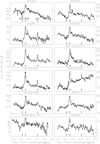 |
Fig. B.1. AKARI 2.5–5 μm spectra of the GOALS sample in the order of their RA and Dec coordinates. The arrows indicate the wavelengths of the 3.1 μm water ice absorption, 3.3 μm PAH emission, and 4.05 μm Brα emission features. |
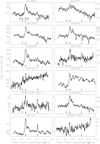 |
Fig. B.1. continued. |
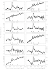 |
Fig. B.1. continued. |
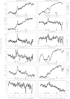 |
Fig. B.1. continued. |
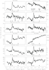 |
Fig. B.1. continued. |
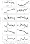 |
Fig. B.1. continued. |
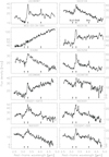 |
Fig. B.1. continued. |
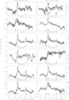 |
Fig. B.1. continued. |
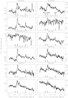 |
Fig. B.1. continued. |
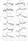 |
Fig. B.1. continued. |
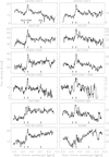 |
Fig. B.1. continued. |
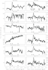 |
Fig. B.1. continued. |
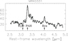 |
Fig. B.1. continued. |
All Tables
Line flux and EQW of 3.3 μm PAH and Brα and the Fν(4.3 μm)/Fν(2.8 μm) color measured in the 4.4″ radius aperture.
Best fit linear coefficients relating 3.3 μm PAH flux to JWST filter color excess from z = 0.0 to z = 5.0.
All Figures
|
Fig. 1. Joined AKARI and Spitzer low-resolution spectra of two typical LIRGs in the sample. The AKARI spectral extraction is performed with the 10.7″ IRS/LL aperture size and the IRS/SL spectra are scaled up to match the LL spectra (see Sect. 3). A starburst-dominated source (CGCG 436-030; top) and an AGN-dominated source (IRAS F08572+3915; bottom) are shown. Their AGN fractions are 8.9 ± 1.8% and 46.6 ± 8.7%, respectively (see Sect. 4.1 and Díaz-Santos et al. 2017). For CGCG 436-030, the fits on the 3.3 μm PAH feature and the Brα line are denoted with red lines. The IRAC 3.6 μm image (1′ × 1′, the same as the AKARI Np FoV size) with the Spitzer IRS SL (red) and LL (blue) apertures overlaid is presented as the inset at the bottom right of each panel. The indicated PAH features in the Spitzer wavelength range are at 6.2, 7.7, 8.6, 11.3, and 12.7 μm in SL, and 16.4 and 17.4 μm in LL. |
| In the text | |
|
Fig. 2. Comparison between AKARI 3.3 μm PAH EQW and Spitzer/IRS 6.2 μm PAH EQW of the GOALS LIRG sample. The circles represent the sources with detections of both PAH features, whereas the left-pointing triangles represent detections of the 6.2 μm PAH but upper limits for the 3.3 μm PAH. The symbols are color-coded by the AGN bolometric fraction in the mid-infrared (Sect. 4.1; Díaz-Santos et al. 2017), which is indicated by the color bar shown in the bottom right. Galaxies with PAH3.3 μm EQW < 0.04 μm and PAH6.2 μm EQW ≥ 0.4 μm are also highlighted by the green squares. The gray regions are the areas where the implied galactic energy source (starburst or AGN) disagrees between 3.3 μm PAH EQW and 6.2 μm PAH EQW (high 3.3 μm PAH EQW but low 6.2 μm PAH EQW, or vice versa). |
| In the text | |
|
Fig. 3. Median spectra of sources with PAH6.2 μm EQW ≥ 0.4 μm, and PAH3.3 μm EQW < 0.04 μm (green; seven objects) or 3.3 μm PAH EQW ≥ 0.04 μm (black; 79 objects). The ranges of the spectra are 1σ uncertainties of the estimated median values. The inset panel shows a zoom-in of the 2.5–5 μm region with the continuum fits in red. The orange arrows indicate the wavelengths where the AKARI continuum color, Fν(4.3 μm)/Fν(2.8 μm), is measured. |
| In the text | |
|
Fig. 4. Ratio of Brα to 3.3 μm PAH emission as a function of decreasing Brα EQW (increasing starburst age, the upper x-axis). The circles represent the sources with both 3.3 μm PAH and Brα detections color-coded by the AGN fraction. The upper limits are shown only for the objects with PAH3.3 μm EQW < 0.04 μm and PAH6.2 μm EQW ≥ 0.4 μm. The starburst ages are derived from the Brα EQW using the Starburst99 models (Leitherer et al. 1999, 2010; Vázquez & Leitherer 2005). |
| In the text | |
|
Fig. 5. Top: ratio of L3.3 μm PAH to LIR 24 as a function of LIR 24. The 3.3 μm PAH emission is measured from the AKARI spectra extracted with the aperture that covers ∼95% of the total flux in the AKARI 2D spectra. We use LIR 24 to denote the total infrared luminosity, scaled by the flux ratio of the Spitzer/MIPS 24 μm emission within the AKARI aperture to the total 24 μm flux (see Sect. 4.3 for more details). The sources with the detected emission feature are shown by the circles. The small gray circles denote the values without the dust extinction correction. The large circles are color-coded by the AGN fraction. The green squares represent the sources with PAH3.3 μm EQW < 0.04 μm and PAH 6.2 μm EQW ≥ 0.4 μm. Bottom: ratio of measured (gray) and corrected (colored) Brα to the infrared luminosity as a function of LIR 24. The horizontal orange solid line and shaded area indicate the mean and its standard deviation of the extinction corrected LBrα/LIR 24, respectively. The horizontal black dashed line indicates LBrα/LIR = 1.56 × 10⁻⁴ when the SFRs derived from LBrα and LIR 24 are the same. |
| In the text | |
|
Fig. 6. PAH6.2 μm EQW plotted against the AKARI 2.5–5 μm continuum slope as measured by the Fν(4.3 μm)/Fν(2.8 μm) ratio (see also Fig. 3). The symbols are the same as in Fig. 2. |
| In the text | |
|
Fig. 7. Ratio of 2MASS K-band to 5 μm monochromatic continuum emission as a function of 3.3 μm PAH EQW. The EQWs are derived from the AKARI spectra extracted with an aperture covering ∼95% of the total AKARI flux. The K-band emission is measured in the imaging data using the same aperture size. The symbols are the same as in Fig. 2, in addition to the red diamonds, which indicate PAH3.3 μm EQW < 0.04 μm and PAH6.2 μm EQW < 0.4 μm. |
| In the text | |
|
Fig. 8. Revised starburst/AGN diagnostic diagram using 3.3 μm PAH EQW and Fν(4.3 μm)/Fν(2.8 μm). The symbols are the same as in Fig. 2. The blue and beige areas are the regions we propose for identifying LIRGs whose infrared continuum emission is dominated by starbursts or AGN, respectively (see also Eqs. (1) and (2)). The white area denotes composite sources (Eq. (3)). |
| In the text | |
|
Fig. 9. Top: JWST filter response curves. The purple and orange curves denote the NIRCam and MIRI filters, respectively. Bottom: median SEDs of starburst- (blue) and AGN-dominated (red) LIRGs. The starburst- and AGN-dominated galaxies are selected to have the AGN fractions <30% and ≥60%, respectively. The SEDs are shown in the rest-frame. The median fluxes are manually scaled to avoid any overlap between the SEDs. The 1.2–2.2 μm, 2.5–5 μm, and 5–38 μm data are from 2MASS, AKARI, and Spitzer, respectively. The redshifted SEDs (z = 0.3–5.0) are shown in Fig. A.1. The SEDs are available as online data at the CDS. |
| In the text | |
|
Fig. 10. AGN infrared color selection with the JWST filters adopted from Lacy et al. (2004; dotted line) and (Donley et al. 2012; solid line). The circles indicate individual LIRGs with the color coding of the AGN fraction shown at the top of the figure. The blue (starburst) and red (AGN) stars indicate the median SEDs from Fig. 9. The panels show the changes of the galaxy colors with the redshift varying from the top (z = 0.0) to the bottom (z = 1.5) in steps of Δz = 0.3. The left column shows the full range of the galaxy color distribution, while the right column shows a magnified portion of the left plot. The plots are shown only up to z = 1.5 due to the wavelength limit (2MASS J-band) of our SEDs being shifted beyond the coverage of F356W. |
| In the text | |
|
Fig. 11. AGN/starburst diagnostic diagrams at each of the redshifts indicated at the bottom left of each panel. The y-axis represents 3.3 μm PAH EQW by taking the flux ratio of the filter covering the 3.3 μm PAH feature to the estimated local continuum emission via a linear interpolation between the two bracketing filters. The x-axis is a measure of hot dust emission. The symbols are the same as in Fig. 10. The vertical dotted line at the colors of 1.5 in each panel indicates an empirical cut for selecting starburst-dominated galaxies. |
| In the text | |
|
Fig. 12. PAH3.3 um fluxes obtained in AKARI spectra compared with an estimate of the 3.3 μm PAH fluxes using three JWST broadband filters from z = 0 to 5.0. At z = 0, the 3.3 μm PAH fluxes are the actual measurements from the AKARI spectra, while for higher redshifts, they are manually scaled to the expected 3.3 μm PAH fluxes of high-z ULIRGs (see text for more details). The broadband estimated PAH fluxes are indicated by the difference between the spectro-photometry in the filter covering the 3.3 μm PAH feature and its local continuum calculated by the linear interpolation of its two neighboring filters. The red solid and dashed lines indicate the best fit line (shown at the top left in each panel) and its 1σ uncertainty, respectively. |
| In the text | |
|
Fig. A.1. Same plots as Fig. 9, but the SEDs are redshifted from z = 0.3 to 5.0 as indicated in each panel. The orange circles on each SED indicate the locations of the effective wavelengths of the JWST filters shown in the upper most panels. |
| In the text | |
|
Fig. B.1. AKARI 2.5–5 μm spectra of the GOALS sample in the order of their RA and Dec coordinates. The arrows indicate the wavelengths of the 3.1 μm water ice absorption, 3.3 μm PAH emission, and 4.05 μm Brα emission features. |
| In the text | |
|
Fig. B.1. continued. |
| In the text | |
|
Fig. B.1. continued. |
| In the text | |
|
Fig. B.1. continued. |
| In the text | |
|
Fig. B.1. continued. |
| In the text | |
|
Fig. B.1. continued. |
| In the text | |
|
Fig. B.1. continued. |
| In the text | |
|
Fig. B.1. continued. |
| In the text | |
|
Fig. B.1. continued. |
| In the text | |
|
Fig. B.1. continued. |
| In the text | |
|
Fig. B.1. continued. |
| In the text | |
|
Fig. B.1. continued. |
| In the text | |
|
Fig. B.1. continued. |
| In the text | |
Current usage metrics show cumulative count of Article Views (full-text article views including HTML views, PDF and ePub downloads, according to the available data) and Abstracts Views on Vision4Press platform.
Data correspond to usage on the plateform after 2015. The current usage metrics is available 48-96 hours after online publication and is updated daily on week days.
Initial download of the metrics may take a while.