| Issue |
A&A
Volume 614, June 2018
|
|
|---|---|---|
| Article Number | A98 | |
| Number of page(s) | 20 | |
| Section | Interstellar and circumstellar matter | |
| DOI | https://doi.org/10.1051/0004-6361/201731690 | |
| Published online | 21 June 2018 | |
Early evolution of viscous and self-gravitating circumstellar disks with a dust component
1
Institute of Fluid Mechanics and Heat Transfer, TU Wien,
1060
Vienna, Austria
e-mail: This email address is being protected from spambots. You need JavaScript enabled to view it.
2
Research Institute of Physics, Southern Federal University,
Stachki Ave. 194,
344090
Rostov-on-Don, Russia
3
Department of Astrophysics, University of Vienna,
Vienna
1180, Austria
4
Institute of Astronomy, Russian Academy of Sciences,
Pyatnitskaya str. 48,
119017
Moscow, Russia
5
Novosibirsk State University,
Lavrentieva str. 2,
630090
Novosibirsk, Russia
6
Boreskov Institute of Catalysis,
Lavrentieva str. 5,
630090
Novosibirsk, Russia
7
European Southern Observatory (ESO),
Karl-Schwarzschild-str. 2,
85748
Garching, Germany
Received:
1
August
2017
Accepted:
18
January
2018
Abstract
Context. Aims. The long-term evolution of a circumstellar disk starting from its formation and ending in the T Tauri phase was simulated numerically with the purpose of studying the evolution of dust in the disk with distinct values of the viscous α-parameter and dust fragmentation velocity vfrag.
Methods. We solved numerical hydrodynamics equations in the thin-disk limit, which were modified to include a dust component consisting of two parts: sub-micron-sized dust, and grown dust with a maximum radius ar. The former is strictly coupled to the gas, while the latter interacts with the gas through friction. Dust growth, dust self-gravity, and the conversion of small to grown dust were also considered.
Results. We found that the process of dust growth that is known for the older protoplanetary phase also holds for the embedded phase of the disk evolution. The dust growth efficiency depends on the radial distance from the star – ar is largest in the inner disk and gradually declines with radial distance. In the inner disk, ar is limited by the dust fragmentation barrier. The process of small-to-grown dust conversion is very fast once the disk is formed. The total mass of the grown dust in the disk (beyond 1 AU) reaches tens or even hundreds of Earth masses as soon as in the embedded phase of star formation, and an even greater amount of grown dust drifts in the inner, unresolved 1 AU of the disk. Dust does not usually grow to radii greater than a few cm. A notable exception are models with α ≤ 10−3, in which case a zone with reduced mass transport develops in the inner disk and dust can grow to meter-sized boulders in the inner 10 AU. Grown dust drifts inward and accumulates in the inner disk regions. This effect is most pronounced in the α ≤ 10−3 models, where several hundreds of Earth masses can be accumulated in a narrow region of several AU from the star by the end of embedded phase. The efficiency of grown dust accumulation in spiral arms is stronger near corotation where the azimuthal velocity of dust grains is closest to the local velocity of the spiral pattern. In the framework of the adopted dust growth model, the efficiency of small-to-grown dust conversion was found to increase for lower values of α and vfrag.
Key words: protoplanetary disks / stars: formation / stars: protostars / hydrodynamics
© ESO 2018
1 Introduction
Circumstellar disks hold the key to our understanding of the star and planet formation process. They serve as a construction site for planets and as a bridge between collapsing pre-stellar cores and nascent stars. In the early evolution phase, properties of circumstellar disks are controlled by a complex interplay between mass-loading from the parental core, energy input from the host star, and mass and angular momentum transport through the disk. If the mass infall rate from the core onto the disk exceeds the total mass loss rate of the disk (through protostellar accretion, jets, disk winds, etc.), the disk grows in mass and size and disk gravitational instability (GI) sets in, leading in some cases to disk fragmentation.
Gravitational instability and disk fragmentation have manifold implications for the evolution of circumstellar disks. Disk fragmentation may account for the formation of giant planets and brown dwarfs, either as companions to host stars or freely floating objects (Boss 2001; Mayer et al. 2002; Boley 2009; Nayakshin 2010, 2017; Vorobyov 2013; Stamatellos 2015). Disk sub-structures formed through GI may serve as likely locations for dust accumulation and growth (Rice et al. 2004; Nayakshin 2010; Gibbons et al. 2015) and notably influence the chemical evolution of young disks (Ilee et al. 2011). Dense gaseous clumps forming in massive GI-unstable disks often migrate into the star, causing strong accretion and luminosity bursts (Vorobyov & Basu 2006, 2015; Meyer et al. 2017), which in turn may have important consequences for protostellar disks and collapsing parental clouds, affecting their gravitational stability, chemical composition, and dust growth (Stamatellos et al. 2012; Vorobyov et al. 2013; Jørgensen et al. 2015; Frimann et al. 2017; Hubbard 2017).
While GI and fragmentation play an important role in the early disk evolution, especially in the embedded phase, other important phenomena, such as the magneto-rotational instability (MRI), can also have a considerable effect on the disk evolution onshort and long timescales. The MRI-induced turbulence can transport mass and angular momentum in the disk regions where ionization is sufficiently high (e.g., Turner et al. 2014), and induce strong accretion and luminosity bursts in the inner disk (e.g., Zhu et al. 2009; Ohtani et al. 2014). However, computing disk evolution with self-consistently induced and sustained MRI turbulence is a challenging task requiring non-ideal magnetohydrodynamics simulations coupled with the stellar radiation input, dust evolution effects, and ionization balance calculations (Akimkin 2015; Ivlev et al. 2016). Such models enable disk simulations only for a limited evolution period and for a narrow set of circumstellar disk parameters (e.g., Flock et al. 2012; Simon et al. 2015). Therefore, numerical simulations adopting the α-prescription of Shakura & Sunyaev (1973) to mimic the effect of turbulent viscosity have been routinely employed to study the long-term evolution of circumstellar disks (e.g., Vorobyov & Basu 2009; Vorobyov 2010; Visser & Dullemond 2010; Rice et al. 2010; Kimura et al. 2016). These simulations have shown the importance of disk self-gravity and viscosity for the evolution and global properties (disk masses, radii) of circumstellar disks.
In this paper, we continue our efforts to study the long-term evolution of self-gravitating and viscous circumstellar disks started in Vorobyov & Basu (2009). We now employ a numerical hydrodynamics code that in addition to the gaseous component also includes the dust component. The evolution of the dust component includes the conversion of small grains into larger grains as a result of coagulation (using the monodisperse growth approach as in Stepinski & Valageas 1997) and drift of the grown dust relative to the gas. Similar modeling of the mutual gas and dust evolution was recently presented in Gonzalez et al. (2017). Our study extends these theoretical efforts by accounting for the self-consistent formation of a circumstellar disk from a parental cloud and by considering the accompanying effect of disk gravitational instability. In this study, we consider the case of a constant α-parameter. Unlike many previous studies of self-gravitating disks with a dust component (Rice et al. 2004; Cha & Nayakshin 2011; Gibbons et al. 2012; Booth & Clarke 2016), we follow the disk evolution starting from its formation from a collapsing pre-stellar core and ending in the early T Tauri phase when essentially all of the collapsing core has dissipated. We specifically study the resulting properties of the gaseous and dusty components of the circumstellar disk, including the efficiency of dust growth, inward drift, and accumulation. Our present development is immediately relevant, since the previous observational studies of a sample of Class 0 young stellar objects have suggested that grain growth begins to significantly change the values of the dust opacity spectral index (β) on 102 AU scales at the ~1–10 mm wavelength range from late Class 0 to early Class II stages (Li et al. 2017). In the later stages of disk evolution, observations indicate dust-to-gas ratios that are higher than the interstellar medium (ISM) value of 0.01, also signifying strong evolution in the disk dust composition (e.g., Williams & Best 2014; Ansdell et al. 2016).
The paper is organized as follows. In Sect. 2 we present the detailed description of our numerical model. The main results are presented in Sect. 3. The parameter space study is conducted in Sect. 4. The model caveats and future improvements are discussed in Sect. 5. The main results are summarized in Sect. 6. Several essential test problems addressing the performance of our numerical scheme on the dust component are shown in Appendix B.
2 Protostellar disk model
The numerical model for the formation and evolution of a star and its circumstellar disk (FEoSaD) is described in detail in Vorobyov & Basu (2015) and Dong et al. (2016). Here, we briefly review its main constituent parts and describe new additions and updates introduced to model the coevolution of a dusty disk. Numerical simulations start from a collapsing pre-stellar core of a certain mass, angular momentum, temperature, and dust-to-gas ratio. The properties of the nascent star are calculated using the stellar evolution tracks derived using the STELLAR evolution code (Yorke & Bodenheimer 2008; Vorobyov et al. 2017), while the formation and long-term evolution of the gaseous and dusty disk components are described using numerical hydrodynamics simulations in the two-dimensional (r, ϕ) thin-disk limit. The evolution of the star and disk are interconnected: the star grows according to the mass accretion rate provided by hydrodynamic simulations and heats the disk according to its photospheric and accretion luminosities.
2.1 Gaseous component
The main physical processes taken into account when modeling the disk formation and evolution include viscous and shock heating, irradiation by the forming star, background irradiation with a uniform temperature of Tbg = 20 K set equal to the initial temperature of the natal cloud core, radiative cooling from the disk surface, friction between the gas and dust components, and self-gravity of gaseous and dusty disks. The code is written in the thin-disk limit, complemented by a calculation of the gas vertical scale height using an assumption of local hydrostatic equilibrium as described in Vorobyov & Basu (2009). The resulting model has a flared structure (because the disk vertical scale height increases with radius), which guarantees that both the disk and envelope receive a fraction of the irradiation energy from the central protostar. The pertinent equations of mass, momentum, and energy transport for the gas component are
 (1)
(1)
![Mathematical equation: \begin{eqnarray*}\frac{\partial}{\partial t} \left( {\mathrm{\Sigma}}_{\textrm{g}} \boldsymbol{v}_p \right) + [\nabla \cdot \left( {\mathrm{\Sigma}}_{\textrm{g}} \boldsymbol{v}_p \otimes \boldsymbol{v}_p \right)]_p & =& - \nabla_p {\cal P} + {\mathrm{\Sigma}}_{\textrm{g}} \, \boldsymbol{g}_p + (\nabla \cdot \mathbf{\Pi})_p, \end{eqnarray*}](/articles/aa/full_html/2018/06/aa31690-17/aa31690-17-eq2.png) (2)
(2)
 (3)
(3)
where subscripts p and p′ refer to the planar components (r, ϕ) in polar coordinates, Σg is the gas mass surface density, e is the internal energy per surface area,  is the vertically integrated gas pressure calculated via the ideal equation of state as
  with γ = 7∕5,
  is the gas velocity in the disk plane, and is
  the gradientalong the planar coordinates of the disk. The gravitational acceleration in the disk plane,
  , takes into accountself-gravity of the gaseous and dusty disk components found by solving for the Poisson integral (see details in Vorobyov & Basu 2010) and the gravity of the central protostar when formed. Turbulent viscosity is taken into account via the viscous stress tensor Π, the expression for which can be found in Vorobyov & Basu (2010). We parameterized the magnitude of kinematic viscosity ν = αcsHg using the alpha prescription of Shakura & Sunyaev (1973) with a constant α-parameter, where cs is the sound speed of gas and Hg is the gas vertical scale height.
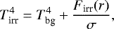
The cooling and heating rates Λ and Γ take the disk blackbody cooling and heating due to stellar and background irradiation into account based on the analytical solution of the radiation transfer equations in the vertical direction (see Dong et al. 2016, for detail):
 (4)
(4)
where  is the midplane temperature, μ = 2.33 is the mean molecular weight,
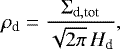
  is the universal gas constant, σ the Stefan-Boltzmann constant, τR = κRΣd,tot∕2 and τP = κPΣd,tot∕2 are the Rosseland and Planck optical depths to the disk midplane, which are calculated from the evolving surface density of total dust population Σd,tot (see Sect. 2.2), and κP and κP (cm2 g−1) are the Planck and Rosseland mean opacities taken from Semenov et al. (2003). We note that the cooling and heating rates in Dong et al. (2016) were written for one side of the disk and need to be multiplied by a factor of 2.
The heating function per surface are of the disk is expressed as
 (5)
(5)
where Tirr is the irradiation temperature at the disk surface determined by the stellar and background blackbody irradiation as
 (6)
(6)
where Firr(r) is the radiation flux (energy per unit time per unit surface area) absorbed by the disk surface at radial distance r from the central star.The latter quantity is calculated as
 (7)
(7)
where γirr is the incidence angle of radiation arriving at the disk surface (with respect to the normal) at radial distance r. The incidence angle is calculated using a flaring disk surface as described in Vorobyov & Basu (2010). The stellar luminosity L* is the sum of the accretion luminosity L*,accr = (1 − ϵ)GM*Ṁ∕2R* arising from the gravitational energy of accreted gas and the photospheric luminosity L*,ph that is due to gravitational compression and deuterium burning in the stellar interior. The stellar mass M* and accretion rate onto the star Ṁ are determined using the amount of gas passing through the sink cell (see Sect. 2.4). The properties of the forming protostar (L*,ph and radius R*) are calculated using the stellar evolution tracks derived using the STELLAR code. The fraction of accretion energy absorbed by the star ϵ is set to 0.1.
2.2 Dusty component
In our model, dust consists of two components: small micron-sized dust, and grown dust. The former constitutes the initial reservoir for dust mass and provides the main input to opacity, and the latter allows us to study dust growth and drift. Small dust is assumed to be coupled to gas, meaning that we only solve the continuity equation for small dust grains, while the dynamics of grown dust is controlled by friction with the gas component and by the total gravitational potential of the star, gaseous and dusty components. Small dust can turn into grown dust, and this process is considered by calculating the dust growth rate and the maximum radius of grown dust. The resulting continuity and momentum equations for small and grown dust are
 (8)
(8)
![Mathematical equation: \begin{align}&\frac{{\partial {\mathrm{\Sigma}}_{\textrm{d},\textrm{gr}} }}{{\partial t}} + \nabla_p \cdot \left( {\mathrm{\Sigma}}_{\textrm{d},\textrm{gr}} \boldsymbol{u}_p \right) = S(a_{\textrm{r}}),\\[8pt]&\frac{\partial}{\partial t} \left( {\mathrm{\Sigma}}_{\textrm{d},\textrm{gr}} \boldsymbol{u}_p \right) + \left[\nabla \cdot \left( {\mathrm{\Sigma}}_{\textrm{d},\textrm{gr}} \boldsymbol{u}_p \otimes \boldsymbol{u}_p \right)\right]_p = {\mathrm{\Sigma}}_{\textrm{d},\textrm{gr}} \, \boldsymbol{g}_p + {\mathrm{\Sigma}}_{\textrm{d},\textrm{gr}} \boldsymbol{f}_p \nonumber \\ &\qquad\qquad\qquad\qquad\qquad\qquad\qquad\ \ \ + S(a_{\textrm{r}}) \boldsymbol{v}_p, \end{align}](/articles/aa/full_html/2018/06/aa31690-17/aa31690-17-eq16.png)
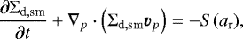
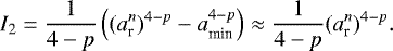
where Σd,sm and Σd,gr are the surface densities of small and grown dust, up describes the planar components of the grown dust velocity, S(ar) is the rate of dust growth per unit surface area, fp is the drag force per unit mass between dust and gas, and ar is the maximum radius of grown dust. To derive the expression for S(ar), we assume a power-law distribution of dust grains over radius N(a) = Ca−p and note that the total dust mass in a specific grid cell does not change through dust growth, so that
 (11)
(11)
where Cn and Cn+1 are the normalization constants, Σd,tot = Σd,gr + Σd,sm is the total surface density of dust, ΔS is the surface area of a specific grid cell, indices  and
and  describe the maximum dust radii at the current and next time steps, amin= 0.005 μm is the minimum radius of small dust grains, and p = 3.5 is the slope of dust distribution over radius (not to be confused with a similar subscript index in Eqs. (1)–(3), (8)–(10), and (20)).
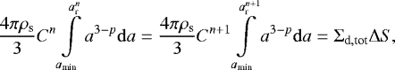
Figure 1 illustrates our dust growth scheme, showing the dust distribution at the current and next time steps n and n + 1 with the red and blue lines, respectively. Here, a* = 1.0 μm is a threshold value between small and grown dust components. The gray area schematically represents the amount of small dust Δ Σd,sm (per surfacearea) converted into grown dust during one hydrodynamic time step Δ t. We note that the area confined between a* and  (highlighted in blue) should also be transferred above
  , but it does not change the mass of grown dust. The corresponding mass per surface area in a specific numerical cell can be expressed as
 (12)
(12)
and the rate of dust growth S(ar) can finally be expressed as
 (13)
(13)
The minus sign reflects the fact that the difference 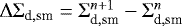 becomes negative when dust grows in a specific cell, that is, when
  . We note that S(ar) is non-zero only if ar > a*. In our models, small dust has radii in the (amin: a*) range, while grown dust has radii in the (a*: ar) range with the temporally and spatially varying maximum radius of grown dust ar. Equation (12) also implicitly allows for conversion of grown dust to small dust as a result of collisional fragmentation if
  . This can occur when grown grains are advected in the disk regions where the fragmentation barrier set by Eq. (26) is lower than the current size of the advected particles. In this case, the radius of dust particles is reduced to match the fragmentation barrier, which formally corresponds to
  and to fragmentation of grown dust back to small dust. Finally, we note that the adopted dust size distribution n(a) = Ca−p is used only to evaluate S(ar) using the total dust density in a specific cell. The individual densities of small and grown dust can also change through advection, and this may produce a discontinuity at a*, which is nottaken into account in the current model.
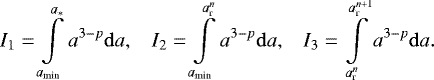
It is worthwhile to analyze how the value of ΔΣd,sm depends on ar. To do this, we express ΔΣd,sm as
 (14)
(14)
where
 (15)
(15)
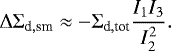
We note that I3 is usually much smaller than I2, because the difference  caused by dust growth during one time step is also small. Under these assumptions, we can write
 (16)
(16)
Noting further that  and making an additional assumption that p < 4, the integral I2 can be written as
 (17)
(17)
Furthermore, because  is small, I3 can be approximated by the following expression:
 (18)
(18)
Noting that I1 is constant, we finally obtain
 (19)
(19)
We verified by numerical integration that Eq. (14) and the approximate formula (19) yield similar results in all the adopted ranges of dust sizes. Therefore, for the adopted power law p = 3.5,  , meaning that the conversion of small into grown dust is more efficient when ar is small.
The evolution of the maximum radius ar is described by the advection equation with a non-zero source term:
 (20)
(20)
where the growth rate  accounts forthe dust evolution that is due to coagulation and fragmentation. We note that when
  is zero, Eq. (20) turns into the Lagrangian or comoving equation for ar, guaranteeing that the bulk motion of grown dust, such as compression or rarefaction, does not change the value of ar in the absence of dust growth. We checked this essential property of Eq. (20) by initiating a gravitational collapse of a cloud core without dust growth and confirmed that ar stays constant and equal to its initial value as the core collapses and the disk forms and evolves.
We write the source term  as
as
 (21)
(21)
where ρd is the total dust volume density, vrel is the dust-to-dust collision velocity, and ρs = 2.24 g cm−3 is the solid (internal) density of grains. The adopted approach is an extension of the monodisperse model of Stepinski & Valageas (1997), so that we use the total dust volume density rather than that of grown dust alone. This allows us to account for collisions not only within the grown dust ensemble, but also between the grown and small dust grains. Because vrel refers to the grown dust, the source term  may be underestimated at the initial stages of dust evolution when the collision velocities are dominated by the fast Brownian motion of small dust grains. However, at the later stages, when the turbulence-induced velocities start to dominate the Brownian motion, the small difference in vrel for grown-to-grown and grown-to-small dust grain collisions (see Fig. 3 in Ormel & Cuzzi 2007) justify the adopted approach. Because the basic dust dynamics is described in terms of the dust surface density, we use the expression
 (22)
(22)
as a proxy for the midplane dust volume density. We note that here we assumed that the scale heights of both small and grown dust are similar, and are equal to the scale height of the grown dust Hd. This assumption can be violated in the presence of efficient dust settling, when small grains are expected to be well mixed with the gas (thus having the same scale height as the gas), but the scale height of the grown dust is expected to be smaller than that of the gas. This effect can decrease the total volume density of dust and the growth rate efficiency. However, as we demonstrate in Sect. 4, dust settling has a lesser effect on dust growth than turbulent viscosity and dust fragmentation barrier. The dust vertical scale height Hd = Hd(ar) is calculated adopting the approach of Kornet et al. (2001; their Eq. (10)), which links the gas and dust vertical scale heights taking the dust sedimentation into account.
The dust-to-dust collision velocity is calculated as 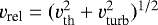 . For the main sources of relative velocities between the dust grains, we consider the Brownian motions with dust collision velocities
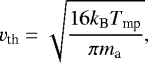 (23)
(23)
and the turbulence-induced velocities (Ormel & Cuzzi 2007; Birnstiel et al. 2012)
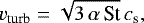 (24)
(24)
where kB is the Boltzmann constant,  is the gas midplane temperature, and ma is the mass of grown dust grains with maximum radius ar. The Stokes number is defined as
 (25)
(25)
where the gas volume density is calculated as  . To summarize the adopted dust growth mechanism, we first calculate the growth rate
  from Eq. (21) using the local quantities in a specific cell. The resulting value of
  is used to update the value of ar using Eq. (20), which in turn is used in Eqs. (13) and (12) to compute the amount of small dust converted into grown dust and the growth rate S(ar).
To simulate the fragmentation of dust grains that is due to mutual collisions, we assume that the maximum radius of a dust grain cannot exceed the fragmentation barrier (Birnstiel et al. 2012), which is defined as
 (26)
(26)
where vfrag is a threshold value for the fragmentation velocity. This effectively means that whenever ar exceeds afrag, the growth rate  is set to zero. We note that even if
  the dust size in a given cell can change as a result of advection, as Eq. (20) implies. The fragmentation velocities of dusty aggregates depend on their properties and may vary in wide limits, typically ~1–10 m s−1 (Dominik & Tielens 1997; Benz 2000; Blum & Wurm 2008). The numerical simulations of collisions between icy dust aggregates suggest vfrag ≈ 20 m s−1 for sintered aggregates (Sirono & Ueno 2014) and vfrag ≈ 50 m s−1 for non-sintered aggregates (Wada et al. 2009). We adopt vfrag = 30 m s−1 in the fiducial model presented in Sect. 3 and explore lower values of vfrag in Sect. 4. In future studies, we plan to adopt a more detailed approach, which will consider the dependence of vfrag on the grain properties, such as their size, ice content, and porosity.
The comparison of the monodisperse growth model of Stepinski & Valageas (1997) with the full-fledged dust growth model was conducted in Birnstiel et al. (2012), showing the validity of the monodisperse approach. However, we wish to point out two possible caveats with this approximation. First, grains that would experience a succession of growth and fragmentation events during their evolution, rather than directly growing to a fragmentation boundary, would reach the limiting size after a longer time. Second, the study of Birnstiel et al. (2012) was applied to older disks (than in the current work), which usually evolve slower than the dust size distribution. Here, we study the early, more dynamical stage of disk evolution, and it is not obvious that the limiting size approximation would also match a more detailed dust evolution since the disk structure evolves much faster. More accurate models of dust evolution need to be employed in the future to test our assumptions. Finally, we note that Pinilla et al. (2016) and Gonzalez et al. (2017) also applied models for calculating the dust evolution in circumstellar disks, which are different in certain aspects. More specifically, the model of Pinilla et al. (2016) uses the full-fledged dust evolution model of Birnstiel et al. (2010), and not the two-population approximation. Gonzalez et al. (2017) used the monodisperse growth model of Stepinski & Valageas (1997) and added fragmentation as a decrease in size each time the relative velocities of grains exceed the fragmentation threshold, instead of limiting the growth to a grain size depending on that threshold.
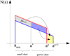 |
Fig. 1 Illustration of the adopted scheme for dust growth. The size distributions of dust grains at the current
n
and next n + 1 time steps are shown with the red and blue lines, respectively. Here, amin
is the minimum radius of small dust grains, while |


2.3 Dragforce
We express the drag force per unit mass between dust and gas following common practice (e.g., Rice et al. 2004; Cha & Nayakshin 2011; Zhu et al. 2012) as
 (27)
(27)
where tstop is the stopping time expressed in the Epstein regime as
 (28)
(28)
Since this approach is valid only for the Epstein drag, we limit the growth of dust in our modeling to a radius ar < 9λ∕4 by manually setting  to zero if this condition is violated. Here, λ is the free mean path of grown dust particles defined as
  , where
  is the mass of hydrogen molecule (Rice et al. 2004). Equation (27) can in principle be used in the Stokes regime for as long as the Reynolds number Re = 4a|up −vp|∕(λcs) is smaller than unity. In this case, tstop needs to be multiplied by 4a∕(9λ). However, the Stokes regime with Re < 1 is usually very narrow. We note that our definition of ar in Eq. (28) implies that we follow the dynamics of dust grains of maximum size, whereas in reality there is a spectrum of grown dust grains between a* and ar. An alternative would be to define ar as a weighted average between a* and ar, in which case the dynamics of an averaged population of grown dust grains would be computed. We defer these and other sophistications of our model to follow-up studies.
2.4 Solution procedure and boundary conditions
Equations (1)–(3), (8)–(10), and (20) are solved using the operator-split solution procedure as described in the ZEUS-2D code (Stone & Norman 1992). The solution is split into the transport and source steps. In the transport step, the update of hydrodynamic quantities due to advection is performed using the third-order piecewise parabolic interpolation scheme of Colella & Woodward (1984). This step also considers the change in maximum dust radius due to advection. We note that the term (up ⋅∇p)a on the r.h.s. of Eq. (20) is not exactly advection, but the derivative along the direction of dust velocity up. However, this term can be recast as advection ∇p ⋅ (aup) minus a correction term a(∇p ⋅up), the latter applied to the solution procedure at the advection step. We finally note that we use the FARGO algorithm to ease the strict limitations on the Courant condition, which occur in numerical simulations of Keplerian disks using the curvilinear coordinate systems converging toward the origin (Masset 2000).
In the source step, the update of hydrodynamic quantities due to gravity, viscosity, cooling, and heating, and also friction between gas and dust components is performed. This step also considers the transformation of small to grown dust and also the increase in dust radius ar due to growth (Eqs. (12)–(20)). To account for the friction terms, we apply the semi-implicit scheme of Cha & Nayakshin (2011) in a modified source step defined as
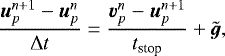 (29)
(29)
where  includes all non-friction terms on the r.h.s. of Eq. (10), and Δ t is the hydrodynamic time step. This equation can be recast in the following form:
 (30)
(30)
This form correctly reproduces the two limiting cases  for tstop → 0 and
  for tstop →∞.
The internal energy per surface area due to cooling Λ and heating Γ is updated implicitly using the Newton-Raphson method of root finding, complemented by the bisection method where the Newton–Raphson iterations fail to converge. The implicit solution is applied to avoid too small time steps that may emerge in regions of fast heating or cooling.
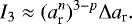
We use the polar coordinates (r, ϕ) on a two-dimensional numerical grid with 256 × 256 grid zones. The radial grid is logarithmically spaced, while the azimuthal grid is equispaced. To avoid too small time steps, we introduce a “sink cell” at rsc = 1.0 AU and impose a transparent inner boundary condition so that the matter (gas or dust) is allowed to flow freely from the active domain to the sink cell and vice versa. The mass of material that passes through the sink cell from the active inner disk at each time step is further redistributed between the growing central star and the sink cell as Δ Mflow = ΔM* + ΔMs.c. (see Fig. 2) according to the following algorithm:

Here, Σs.c. is the surface density of gas/dust in the sink cell,  the averaged surface density of gas/dust in the inner active disk (the averaging is usually done over several AU immediately adjacent to the sink cell, the exact value is determined by numerical experiments), and Ss.c. the surface area of the sink cell. The exact partition between ΔM* and ΔMs.c. is usually set to 95:5%. We note that if ΔMflow < 0, the material flows out of the sink cell into the active disk. In this case, we update only the surface density in the sink cell as
 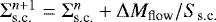 and do not change the mass of the central star.
The calculated surface densities in the sink cell  are further used as boundary values for the surface densities in four inner ghost zones, which have the size of the corresponding active grid cells on the other side of the sink cell interface and are needed for the piecewise parabolic advection scheme used in the code. The radial components of velocities in the inner ghost zones are set equal to their immediate counterparts in the active disk, while the azimuthal components in the inner ghost zones are extrapolated assuming Keplerian rotation as
 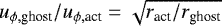 , where uϕ,act is the ϕ-component of velocity in the innermost active zones, and ract and rghost the radial positions where ϕ-components of velocities are defined in the active and ghost zones, respectively.
These boundary conditions enable a smooth transition of surface density between the inner active disk and the sink cell, preventing (or greatly reducing) the formation of an artificial drop in the surface density near the inner boundary. We ensure that our boundary conditions conserve the total mass budget in the system. Finally, we note that the outer boundary condition is set to a standard free outflow, allowing for material to flow out of the computational domain, but not allowing any material to flow in.
The code was tested on the test problems applicable to the polar geometry, showing good performance on the relaxation and angular momentum conservation problems (Vorobyov & Basu 2006). A small amount of artificial viscosity added to the code to smooth shocks produces artificial torques that are many orders of magnitude smaller than the physical gravitational and viscous torques (Vorobyov & Basu 2007). Additional tests pertinent to the dust component are presented in the appendix.
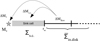 |
Fig. 2 Schematic illustration of the inner boundary condition. The mass of material Δ Mflow that passes through the sink cell from the active inner disk is further divided into two parts: the mass Δ M* contributing to the growing central star, and the mass ΔMs.c. settling in the sink cell. |
2.5 Initial conditions
Our numerical simulations start from a pre-stellar core with the radial profiles of column density Σg and angular velocity Ωg described asfollows:
![Mathematical equation: \begin{eqnarray} {\mathrm{\Sigma}}_{\textrm{g}} (r) & = & {r_0 {\mathrm{\Sigma}}_{0,\textrm{g}} \over \sqrt{r^2+r_0^2}}\:,\\ {\mathrm{\Omega}}_{\textrm{g}} (r) & = &2 {\mathrm{\Omega}}_{0,\textrm{g}} \left( {r_0\over r}\right)^2 \left[\sqrt{1+\left({r\over r_0}\right)^2 } -1\right],\end{eqnarray}](/articles/aa/full_html/2018/06/aa31690-17/aa31690-17-eq71.png)
where Σ0,g and Ω0,g are the gas surface density and angular velocity at the center of the core. These profiles have a small near-uniform central region of size r0 and then transition to an r−1 profile; they are representative of a wide class of observations and theoretical models (André 1993; Dapp & Basu 2009). The core is truncated at rout = 0.045 pc, which is also the outer boundary of the active computational domain (the inner boundary is at rs.c. = 1 AU). The initial dust-to-gas ratio is set to 0.01, and it is assumed that only small dust is initially present in the core (Σd,gr is initially set to a negligibly low value). The radial profiles of the surface density and angular velocity of small dust are then defined as Σd,sm(r) = 0.01Σg(r) and Ωd,sm(r) = Ωg(r). The initial gas temperature is set to 20 K throughout the core.
The initial parameters Σ0,g = 0.2 g cm−2 and r0 = 1200 AU are chosen so that the core is gravitationally unstable and begins to collapse at the onset of numerical simulations. The total initial mass of the core is Mcore = 1.03 M⊙ and the adopted initial value of Ω0,g = 1.8 km s−1 pc−1 results in the ratio of rotational-to-gravitational energy β = 0.24%, typical for pre-stellar cores (Casselli et al. 2002).
3 Main results
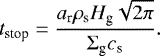
In this section, we study the long-term evolution of a circumstellar disk formed during the gravitational collapse of our model cloud core. The disk forms at t = 0.055 Myr, and the numerical simulations are terminated at t = 0.5 Myr. The time is counted from the onset of gravitational collapse (which is also the onset of numerical simulations). The embedded phase of star formation defined as the time period when the mass in the envelope is greater than 10% of the total initial mass in the core ends around t = 0.15 Myr. We therefore cover the entire embedded phase of disk evolution plus some of the Class II phase. The free parameters of our fiducial model are as follows: α = 0.01 and vfrag = 30 m s−1. We also take dust settling into account. The effect of varying free parameters is considered in Sect. 4.
Figure 3 presents the gas surface density distribution Σg in the inner 1000 × 1000 AU2 box. The computational domain covers a much larger area (~104 × 104 AU2), including the infalling envelope, but we show only the most interesting inner region, which covers the evolving disk. The central star forms at t = 0.053 Myr and the diskforms about 2 kyr later. The sequence of images illustrates how the disk grows with time and changes its shape from compact and non-axisymmetric in the embedded phase to extended and practically axisymmetric in the Class II phase. In the embedded phase of evolution, the disk is gravitationally unstable thanks to continuing mass-loading from the infalling envelope, which results in the development of a notable spiral structure and even leads to episodic fragmentation. The inset at t = 0.15 Myr zooms on to the gaseous clump in the 150 × 150 AU2 box. To determine whether the disk fulfills the Toomre fragmentation criterion, we adopted the modified definition of the Q-parameter that is appropriate for the near-Keplerian disks. The black contour line outlines the region where the Toomre parameter QT calculated using the following equation is less than unity:
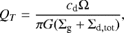 (33)
(33)
where  is the modified sound speed in the presence of dust and ξ = Σd,tot∕Σg the total dust-to-gas ratio. Clearly, the element of the spiral arm where fragmentation took place is Toomre-unstable. We defer a more rigorous analysis of disk fragmentation and clump properties including their dust content to a follow-up study with higher resolution. In the T Tauri phase, the disk is characterized by a regular spiral structure, which slowly diminishes as the disk loses its mass through accretion onto the star. Concurrently, the disk spreads out as a result of the action of viscous torques (Vorobyov & Basu 2009).
In Fig. 4 we show the zoomed-in images of the gas surface density (first row), surface density of grown dust (second row), gas-to-grown dust mass ratio Σg∕Σd,gr (third row), Stokes number (fourth row), and maximum radius of grown dust (bottom row) at t = 0.2 Myr. In particular, the left, middle, and right columns zoom on the inner 200 × 200 AU2, 60 × 60 AU2, and 10 × 10 AU2 disk regions, respectively. The contour lines of Σg in the third and fourth rows of Fig. 4 outline the position of the spiral arms, which serve as a proxy for the position of pressure maxima (spiral arms are both denser and warmer than the inter-arm regions). A comparison of the first and second rows indicates that the spatial distribution of grown dust generally correlates with the spatial distribution of gas in the sense that both exhibit a similar spatial pattern. The third row demonstrates that the inner disk is characterized by lower values of Σg ∕Σd,gr than the outer disk, reflecting the process of gradual inward drift of grown dust grains. We note that the spatial distribution of the relative content of small-to-grown dust Σd,sm∕Σd,gr is similar to that of gas-to-grown dust Σg∕Σd,gr (but is lower by about a factor of 100) because small dust follows gas in our model.
The situation with spiral arms as the pressure maxima and the likely places of dust accumulation is more complicated. The spiral arms in the outer disk are on average characterized by lower values of Σg ∕Σd,gr than the inter-arm regions (left panel in the third row). At the same time, the accumulation of grown dust in the inner disk that is due to inward radial drift is more pronounced than accumulation of dust in the spiral arms (middle and right panels in the third row). The fourth row of Fig. 4 indicates that the spiral arms are characterized by low Stokes numbers, which can be explained by higher gas densities and temperatures in the spiral arms than in the inter-arm regions. We note that the Stokes number in the Epstein regime also depends linearly on the grain size, but a mild increase of ar in the spiral arms is insufficient to compensate for a stronger increase in gas density and temperature (see also Fig. 6), so that the Stokes number effectively decreases. As numerical studies of dust dynamics in gravitationally unstable disks indicate (Gibbons et al. 2012; Booth & Clarke 2016), the dust concentration efficiency depends on the Stokes number and is highest for the Stokes number on the order of unity. For Stokes numbers <0.1, the concentration of dust grains in pressure maxima may be a slow process (because of rather efficient coupling with gas), comparable to or longer than the lifetime of the spiral pattern in our simulations.
Figure 5 presents the relative velocities between the grown dust and gas components superimposed on the gas surface density map. We zoom in on one of the spiral arms in the disk (stretching from the upper left to the bottom right corner) to illustrate the dust drift in the vicinity of pressure maxima as represented by the spiral arm. The overall inward drift of grown dust toward the spiral arm is clearly visible. The relative drift velocities are higher at the edges of the spiral because of lower gas densities and, hence, weaker gas-to-dust coupling.
To illustrate the varying efficiency of grown dust concentration in the inner and outer spiral arms, we plot in Fig. 6 the surface densities of gas (red solid lines), small dust (blue dashed lines), and grown dust (black solid lines) taken along the azimuthal cuts at different distances from the star: r = 20 AU, r = 50 AU, r = 82 AU, and r = 150 AU. We also plot the azimuthal profiles of the gas pressure and maximum radius of dust grains ar. Spiral arms manifest themselves as local peaks in the gas surface density and pressure. The contrast in the surface density and pressure between the spirals and the inter-arm regions is smaller and the pressure maxima are less sharp in the inner disk regions. The azimuthal variations in pressure can weaken in the inner disk because spiral arms converge and wind up toward the disk center, as Fig. 4 indicates. This can also be caused by a weakened GI, but only in the innermost 10–15 AU, where the Q-parameter (see Fig. 11) becomes greater than 2.0. Clearly, the azimuthal distribution of small dust follows that of gas at all radial distances. On the other hand, the behavior of grown dust is distinct from that of small dust. The contrast in the grown dust density between the spiral arms and the inter-arm regions increases at larger distances and becomes higher by about a factor of two than the corresponding contrast in the gas surface density. At r = 82 AU, for instance, Σd,gr is factors of 35 and 5 higher in the center of the spiral arm (ϕ ≈ 3.0 rad) than in the immediate inter-arm region on the left- and right-hand sides from the arm, respectively. The corresponding factors for Σd,sm are 18 and 6. This implies accumulation of grown dust in the outer parts of spiral arms. ar shows little correlation with the spiral arms in the innermost and outermost disk regions (20 and 150 AU, respectively). In the intermediate disk regions (50 and 82 AU), some increase in ar at the positions of spiral arms is evident, which is likely due to faster growth in high-density regions. However, this increase (maximum a factor of two) is insufficient to compensate for the corresponding increase in the gas surface density and temperaturein the spiral arms, so that the Stokes numbers decrease in the spiral arms (see also Fig. 4).
To understand why grown dust preferentially accumulates in the outer parts of the spiral arms, we compare the characteristic velocities of dust drift udrift with the velocity of dust in the local frame of reference of the spiral pattern up −vsp. The components of the drift velocity can be approximated as (Birnstiel et al. 2016)
 (34)
(34)
where vK is the Keplerian velocity and η defines the deviation of the gas rotation velocity from the purely Keplerian law  . In the region of interest (r < 200 AU), the Stokes number varies between 0.01 and 0.2 (see Fig. 8), so that the dust drift is dominated by the azimuthal component uϕ,drift. The bulk velocity of dust is also dominated by the azimuthal component uϕ, and in the following analysis, we consider only the azimuthal flow.
Figure 7 presents the radial profiles of |uϕ,drift|, uϕ − vsp, their ratio ζ = |uϕ,drift|∕|uϕ − vsp|, and the parameter η at t = 0.2 Myr. The velocity of the spiral pattern vsp is calculated by taking the azimuthal cuts at 50 yr intervals and finding the angular velocity with which the peaks in the gas density (spiral arms) propagate at a given radial distance. When calculating the Keplerian velocity, we also take into account the enclosed disk mass because our model disk is self-gravitating. The efficiency of dust accumulation in spiral arms is highest in the regions where ζ is highest because in these regions, the drift velocity dominates the bulk velocity of dust in the local frame of reference of the spiral pattern. These are also the regions where the spiral pattern nearly corotates with the azimuthal dust flow. We note that uϕ − vsp is positive in the inner disk and negative in the outer disk, which reflects the change in azimuthal dust flow near corotation – dust moves faster than the spiral pattern inside corotation and slower outside corotation. The value of ζ drops at small radial distances, which explains why the accumulation of grown dust in the spiral arms of the inner disk regions is inefficient. We note that η is higher than what is usually assumed for axisymmetric circumstellar disks (e.g., a few per mille, see Birnstiel et al. 2016), which is likely due to perturbations that the spiral arms cause in the gas flow. Finally, we note that uϕ,drift weakly depends on the Stokes number for St < 1.0, and some concentration of small dust particles in the spiral arms can also be expected. This cannot be verified in our models since we assume that small dust moves with the gas, but it needs to be investigated in future studies.
We conclude that the concentration of dust grains in the spiral arms is most efficient near the corotation region, where the azimuthal velocity of dust grains is closest to the local velocity of the spiral pattern and the ratio ζ of the dust drift velocity to the dust azimuthal velocity in the local frame of reference of the spiral pattern is highest. The inner parts of the spiral arms are characterized by moderate pressure maxima and low values of ζ so that a clear dust concentration does not have time to form. We also note that our multi-armed spiral pattern is rather transient, as is also evident from Fig. 3. Dust accumulation in spiral arms is expected to be more efficient in the presence of a grand-design, two-armed spiral pattern, as was observed in Elias 2–27 (Pérez et al. 2016; Tomida et al. 2017), given that these structures live much longer than we found in our simulations.
To further analyze the dust dynamics, we plot in Fig. 8 the surface densities of small and grown dust (Σd,sm and Σd,gr, respectively), the maximum radius of grown dust (ar), and the Stokes number (St) as a function of gas surface density (Σg) at t = 0.2 Myr. Only the data for the inner 200 AU around the star were used. The black solid lines illustrate the linear and quadratic functional dependence on Σg. Clearly, Σd,sm follows the expected linear dependence on Σg because of the strict coupling between these components. A mild weakening of the Σd,sm vs. Σg dependence in the high-gas-density limit can be explained by a more efficient conversion of small grains into large ones in the denser inner disk. The surface density of grown dust Σd,gr, on the other hand, reveals a more complicated pattern with the linear dependence on Σg at the low-density tail and a quadratic or even steeper dependence in the high-gas-density limit. The likely explanation for this phenomenon is the inward radial drift, which increases the relative abundance of grown dust in the inner disk regions that are characterized by the highest gas surface densities. Moreover, the surface density of grown dust approaches that of small dust at the highest Σg (i.e., in the innermost disk parts). The Stokes numbers anticorrelate with the gas surface density, as was already noted in Fig. 4. This trend is especially pronounced in the high-gas-density limit. The maximum radius of dust grains ar shows a more complicated pattern – it grows with Σg in the low and intermediate gas-density regime, but saturates or even drops in the high gas-density limit. As we demonstrate below, this behavior is caused by grown dust reaching the fragmentation barrier in the inner disk.
Figure 9 presents the azimuthally averaged radial profiles of gas surface density (blue solid lines, first row), gas midplane temperatureTmp (blue solid lines, second row), surface densities of small dust grains and grown dust (blue dashed and solid lines, third row), and maximum radius of dust grains (blue solid lines, bottom row). The black dashed and dash-dotted lines in the second row show the gas midplane temperatures that would be expected in the presence of either stellar and background irradiation or viscous heating only, respectively. The black dashed line in the bottom row represent the fragmentation barrier. The same time instances as in Fig. 3 are shown: t = 0.2 Myr (left column) and t = 0.4 Myr (right column). In the early evolution at t = 0.2 Myr, a piecewise radial distribution of gas surface density is evident, with a shallower profile in the inner parts of the disk and a steeper profile in the outer disk. This form of Σg(r) can be expected for disks whose properties are governed by viscous transport in the inner (hotter) disk regions and by gravitational instability in the outer (colder) regions (e.g., Lodato & Rice 2005; Vorobyov & Basu 2009). The second row demonstrates that the gas temperature in the outer disk is controlled by the stellar and background irradiation, while in the inner disk regions (r < 25 AU), viscous heating greatly dominates heating as a result of stellar and background radiation, and viscosity becomes the dominant transport mechanism. In the later evolution at t = 0.4 Myr, the radial profile of Σg loses its piecewise shape. At this stage, gravitational instability subsides (as is evident in Fig. 3) and the disk dynamics is governed mostly by viscous torques. These torques act to spread out the disk outer parts, leading to the gas surface density profile that is better described by an exponent than by a piecewise power law (Lynden-Bell & Pringle 1974; Vorobyov 2010).
The third row in Fig. 9 describes the azimuthally averaged characteristics of the dusty disk component. The radial distribution of small dust Σd,sm follows that of gas, but the radial distribution of grown dust shows notable deviations from that of gas because of inward drift. The increase of Σd,gr toward the star is faster than that of Σd,sm, so that the ratio Σd,gr∕Σd,sm gradually rises at smaller radii. At a radial distance of a few AU, Σd,gr becomes comparable to Σd,sm. The total dust-to-gas ratio ξ shown by the red dash-dotted line, however, does not show significant deviations from the initial value of 0.01. Small grains vastly dominate the dust disk mass in the disk regions beyond 1.0 AU. This is a consequence of efficient inward drift of grown dust and continuing replenishment of small dust from the infalling envelope in the embedded phase of disk evolution.
Finally, the bottom row presents the radial profile of the maximum dust radius ar. Clearly, the maximum growth occurs at r = 20–40 AU, where ar becomes as large as several centimeters. In fact, the growth at smaller distances is limited by the fragmentation barrier, as was also found in Gonzalez et al. (2015), for example. At larger distances r≳100 AU, however, dust does not grow to the fragmentation barrier and hardly exceeds 1.0 mm in radius.
Figure 10 presents various integrated characteristics in our model. In particular, the top panel shows the masses of gas in the disk and envelope and the stellar mass as a function of time. The bottom panel shows the masses of small and grown dust in the disk and also the mass of dust that passed through the sink cell. We note that the masses of gas and dust in the disk are calculated only for the disk regions beyond rsc = 1.0 AU, that is, for the disk regions that are resolved in our numerical simulations. The mass of gas in the disk becomes as high as 0.3 M⊙ in the embedded phase (t ≤0.15 Myr) and gradually declines afterward. The mass of grown dust in the disk reaches 60 Earth masses in the embedded phase and drops to 30 Earth masses in the T Tauri phase as a result of protostellar accretion. At the same time, the mass of small dust in the disk (≤ 1.0 μm) approaches 1000 Earth masses in the embedded phase and gradually declines to 600 Earth masses at t = 0.5 Myr, meaning that most of the total dust mass in the disk beyond 1.0 AU remains in the form of small dust grains. This can also be seen from the third row of panels in Fig. 9. At the same time, the mass of grown dust that passed through the sink cell is much higher than what remains in the active disk. In fact, the masses of small and grown dust that have passed through the sink by the end of simulations (t = 0.5 Myr) are comparable. This means that our fiducial model with α = 0.01 and vfrag = 30 m s−1 is rather efficient in converting small to grown dust, but most of grown dust quickly drifts in the innermost, unresolved disk regions. The fast inward drift of grown dust and continuing replenishment of small dust from the infalling envelope (in the embedded phase) explains why the small dust grains vastly dominate the disk mass beyond 1.0 AU. We note that the process of small-to-grown dust conversion is very fast once the disk forms at t ≈ 0.056 Myr. The mass of grown dust reaches 40 Earth masses at 10 kyr after disk formation and a local maximum of 60 Earth masses at 46 kyr after disk formation.
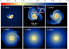 |
Fig. 3 Gas surface density distribution in the inner 1000 × 1000 AU2 box at six evolutionary times starting from the onset of gravitational collapse. The inset shows the fragments formed in the disk via gravitational fragmentation. The black line in the inset highlights the region where the Toomre parameter is less than unity. The scale bar is in log g cm−2. |
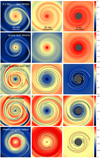 |
Fig. 4 Zoom-in onto the inner disk regions at t = 0.2 Myr: left column –200 × 200 AU2, middle column – 60 × 60 AU2, and right column – 10 × 10 AU2. Shown are the gas surface density in log g cm−2 (top row), grown dust surface density in log g cm−2 (second row), gas-to-grown dust mass ratio in log scale (third row), Stokes number in log scale (fourth row), and maximum radius of dust grains ar in log cm. The contour lines in the third, fourth, and fifth rows delineate the spiral pattern in the gas surface density for convenience. |
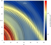 |
Fig. 5 Velocity field for grown dust (relative to the gas) superimposed on the gas surface density map in the vicinity of a prominent spiral arm at t = 0.2 Myr. |
 |
Fig. 6 Surface densities of gas (red solid lines), small dust (blue dashed lines), and grown dust (black solid lines) taken along the azimuthal cuts at different distances from the star: r = 20 AU, r = 50 AU, r = 82 AU, and r = 150 AU. The dashed pink and solid cyan lines show the gas pressure (in the code units) and the maximum radius of dust grains ar (in cm) taken along the same cuts. The evolution time is t = 0.2 Myr. We applied different scaling factors for the small dust density, grown dust density, and maximum dust radius. |
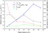 |
Fig. 7 Radial profiles of the azimuthal component of the dust drift velocity |uϕ,drift|, the azimuthal component of the dust bulk velocity relative to the local velocity of the spiral pattern uϕ − vsp, their ratio ζ = |uϕ,drift|∕|uϕ − vsp|, and the parameter η. |
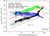 |
Fig. 8 Surface density of grown dust, maximum radius of dust grains, and Stokes number as a function of the gas surface density within 200 AU from the star at t = 0.2 Myr. The black solid lines illustrate the linear and quadratic dependencies to facilitate comparison. |
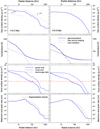 |
Fig. 9 Azimuthally averaged radial profiles of the gas surface density (blue solid lines, top row), gas midplane temperature (blue solid lines, second row), surface densities of small and grown dust (blue dashed and solid lines, third row), and maximum radius of grown dust (blue lines, bottom row) at two evolutionary times: t = 0.2 Myr (left column) and t = 0.4 Myr (right column). The dotted lines present various dependencies on radial distance r to facilitate comparison. The black dashed and dash-dotted lines in the second row show the gas midplane temperatures that would be expected in the presence of either stellar + background irradiation or viscous heating only, respectively. The red dash-dotted lines in the third row are the total dust-to-gas mass ratio. Finally, the black dashed lines in the bottom row present the fragmentation barrier. |
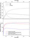 |
Fig. 10 Toppanel: integrated masses of the disk and envelope (solid and dash-dotted line) and the mass of the central star (dashed line) as a function of time. Bottom panel: total masses of the grown dust (blue solid line) and small dust (red solid line) in the disk as a function of time. We also show the masses of small and grown dust that passed through the sink cell (red dashed and blue dashed lines, respectively). |
4 Parameter space study
In this section, we study the effect of free parameters in our models on the distribution of grown dust in the disk. In particular, we consider a lower value of α =0.001 and lower values of the fragmentation velocity vfrag = 10 m s−1 and vfrag = 20 m s−1. In addition, we consider a model without dust settling, which is motivated by the study of Rice et al. (2004), who found that vertical stirring in a gravitationally unstable disk prevents dust particles from settling to the midplane. This effectively means that the dust vertical scale height Hd is set equal to the vertical scale height of gas Hg.
Figure 11 presents the azimuthally averaged radial profiles of the maximum radius ar in models with different α-parameters and fragmentation velocities at t = 0.2 Myr. More specifically, the top left panel corresponds to the fiducial model with α =0.01 and vfrag = 30 m s−1. Other panels correspond to models with α = 10−3 and vfrag = 30 m s−1 (top right), α = 0.01 and two values of vfrag = 10 m s−1 and vfrag = 20 m s−1 (bottom left; top curves correspond to vfrag = 20 m s−1) and to the model with α = 0.01 and vfrag = 30 m s−1, but without dust settling (bottom right). The solid blue lines are the model results, and the dashed black lines are the maximum grain radius afrag set by the fragmentation barrier.
In the fiducial model, the dust radius does not exceed a few centimeters in the innermost disk, slightly increases at 10–30 AU, and gradually declines at larger radii. In the inner 30 AU, the dust growth is clearly limited by the fragmentation barrier, whereas at larger radii, the dust growth is either slow or limited by inward drift. Turbulence affects dust growth in several ways. First, it facilitates dust growth via an increased collision rate. However, too high grain-grain relative velocities lead to destructive collisions. We do not follow individual trajectories of dust particles and a succession of dust growth and fragmentation events. Instead, our dust growth model includes a limitation on the grain size as described by Eq. (26), which implicitly takes the destructive effect of turbulence into account, although in a simplified manner. Second, turbulence affects transport processes and, hence, the disk density and velocity structure. Third, dust grains are efficient absorbers of free electrons (Ivlev et al. 2016) and can modulate the ionization fraction and the development of the MRI. It is therefore non-trivial to predict the exact effect of turbulence on dust growth.
The maximum growth of dust grains is found in the α = 10−3 model, which can be explained by a lower turbulence (and lower α) and denser inner disk, both causing the fragmentation barrier to increase. The gas density in the inner disk of the α = 10−3 model increases because of the decreased viscous mass transport. We illustrate this phenomenon in Fig. 12 by comparing the radial profiles of the gas surface density, viscous torques, and gravitational torques in the α = 10−3 model with the corresponding radial profiles in the fiducial model (α = 10−2) at t = 0.2 Myr. We focus on the inner disk regions where the difference in the maximum grain size is most pronounced. The net gravitational and viscous torques at a given radial distance r are found by summing all local viscous and gravitational torques defined as
where m(r, ϕ) is the gas mass in a cell with polar coordinates (r, ϕ), Φ is the gravitational potential, and S(r, ϕ) is the surface area occupied by a cell with polar coordinates (r, ϕ). The summation is performedover the polar angle ϕ for grid cells with the same radial distance r. To reduce noise, the resulting torques were further averaged over a time period of 200 yr. Clearly, the viscous torques in the α =10−3 model are systematically lower (by absolute value) than in the fiducial model. Moreover, positive values of the viscous torques are seen in bothcases, but at different radii, and are to be expected when spiral arms are present. At the same time, the gravitational torques in both models are negligible (as compared to the viscous ones) in the inner 7 AU for the α =10−3 model and in the inner 20 AU in the fiducial model because the GI in the inner, hot disk regions is weaker (see, e.g., Fig. 4). This is also evident from the radial profiles of the Toomre Q-parameter shown by the red lines in Fig. 11. As a result, mass transport in the inner 10 AU of the α =10−3 model is less efficient, causing matter to accumulate in the inner disk and raising the gas surface density. A similar trend of higher Σg, lower τvisc and negligible τgr in the α = 10−3 model holdsat later evolutionary times. In this model, dust can grow to meter-sized boulders in the inner 10 AU. Beyond 10 AU, however, the maximum radius of dust grains drops notably below afrag. In the models with lower values of the fragmentation velocity shown in the bottom left panel of Fig. 11, the dust radius is notably smaller than in the fiducial model with vfrag = 30 m s−1, which is clearly caused by a lower fragmentation barrier. We conclude that low values of α, together with high values of vfrag, are needed for dust grains to grow to radii greater than a few cm. Finally, we note that the presence or absence of dust settling has little effect on the size of dust grains in the inner disk where the grain size is limited by the fragmentation barrier, which does not depend on the dust volume density (see Eq. (26)). In the outer disk, the grain size in the model without settling is slightly lower than in the model with settling because dust growth depends linearly on the volume density of dust grains (see Eq. (21)) and ρd is higher in the case with dust settling.
Figure 13 presents other results of our parameter space study. In particular, the first two rows show the total dust mass in the disk as a function of time for the fiducial model with α =10−2 and vfrag = 30 m s−1 (top left), for the model with α = 10−3 and vfrag = 30 m s−1 (top right), for the model with α = 10−2 and vfrag = 20 m s−1 (middle left), and for the model with α = 10−2 and vfrag = 10 m s−1 (middle right). The bottom row presents the ratio of enclosed dust masses Md,gr(r)∕Md,sm(r) as a function of radial distance r at different evolution times for the fiducial model and for models with varying free parameters. Clearly, reducing the α-parameter has a notable effect on the total mass of grown dust in the disk, which is higher by about an order of magnitude by the end of numerical simulations as compared to the fiducial case of α =0.01. The increase is caused by inefficient mass transport in the inner 10 AU. The resulting pile-up of grown dust in the inner disk (relative to small dust, which traces the gas distribution) is clearly seen in the ratio Md,gr(r)∕Md,sm(r) shown by the blue lines in the bottom row of Fig. 13. It is an interesting finding, showing that the pile-up of grown dust can occur even for constant but sufficiently low viscous α ≤10−3 in circumstellar disks with a radially varying strength of GI. There is also a clear tendency for the increase in the ratio of enclosed masses toward the star. This trend becomes more pronounced with time, reflecting a gradual inward driftof grown dust. Our numerical findings are in agreement with recent observations of the FU Orionis system using VLA, which have found that millimeter- and centimeter-sized dust is localized in the inner several AU (Liu et al. 2017).
It is interesting that decreasing vfrag (and making grains more prone to destruction) has a similar effect – the mass of grown dust in the disk has increased by about an order of magnitude as compared to the fiducial model. The effect is especially pronounced in the ratio of enclosed masses Md,gr(r)∕Md,sm(r) shown in the bottom row of Fig. 13. In the fiducial case with vfrag = 30 m s−1, the ratio Md,gr(r)∕Md,sm(r) is about unity in the innermost disk and gradually declines at larger radii. In the vfrag = 20 m s−1 model, this ratio is already greater than unity in the inner 10 AU and increases sharply in the innermost disk regions, indicating a more efficient conversion of small to grown dust for lower values of vfrag. In the vfrag = 10 m s−1 model, the inner several AU are completely depleted of small dust grains. This counterintuitive effect of increased small-to-grown dust conversion for lower values of vfrag is caused by a juxtaposition of two factors: an increased efficiency of small-to-grown dust conversion for lower values of ar and inward drift of grown dust grains. Decreasing vfrag acts to decrease the maximum radius ar because the fragmentation barrier is lower (see Fig. 11). This in turn increases the conversion efficiency of small to grown grains because S(ar) increases as ar decreases (see Eq. (19)). The grown dust drifts inward and grains with smaller ar from outer disk regions take their place, thus sustaining a cycle of dust growth.
We further illustrate this phenomenon in Fig. 14, showing the azimuthally averaged profiles of the Stokes number (top panel), surface density of grown dust (middle panel), and integrated masses of grown dust that passed through the sink cell and remaining in the disk (bottom panel) in models with vfrag = 10 m s−1 and vfrag = 30 m s−1. The Stokes numbers are systematically lower in the vfrag = 10 m s−1 model because of smaller ar, indicating a slower radial drift of grown dust. A less efficient dust drift in the vfrag = 10 m s−1 model can also be seen from the ratios Md,gr(disk)∕Md,gr(total) of the grown dust mass in the disk to the total produced mass of grown dust (that residing in the disk and passed through the sink cell). These ratios are 7.5 and 2.2% for the vfrag = 10 m s−1 and vfrag = 30 m s−1 models, respectively. This indicates that low vfrag models can be described as causing a better retention of grown dust in the disk, as opposed to favoring a more efficient dust growthand reaching larger dust sizes. As a result, the gas surface density of grown dust increases in the vfrag = 10 m s−1 model, as is shown in the middle panel of Fig. 14. In both models, the amount of grown dust that passed through the sink cell in the inner (unresolved) 1 AU is notably higher than what remains in the rest of the disk. We note that without inward dust drift, this mechanism of efficient small-to-grown dust conversion and dust accumulation would not work. We note that fast conversion of small to grown dust grains in the innermost disk regions was also reported by Birnstiel et al. (2010), who used a more sophisticated dust growth scheme, but considered a semi-analytic prescription for disk dynamics.
We emphasize that in all models, the process of small-to-grown dust conversion is very fast. As Fig. 13 indicates, the mass of grown dust reaches tens or even hundreds of Earth masses already by the end of the embedded phase at t = 0.15 Myr. In the model with α = 10−3, the mass of grown dust continues to increase in the early T Tauri stage, while it slowly decreases in the other models. The radial distribution of grown dust is, however, distinct in different models. Figure 15 shows the enclosed mass of grown dust Md,gr(r) as a function of radial distance at t = 0.2 Myr. In the α = 10−3 model, almost all grown-dust mass is concentrated in the inner several AU, while other models are characterized by a notably smoother radial distribution of grown-dust mass. It might be hard to detect grown dust in the α =10−3 model because the absolute mass in grown dust grains outside of the inner several AU is very limited. We note that the total mass of grown dust of several hundred Earth masses concentrated in a narrow inner region with a width of several AU (as in the α =10−3 model) may be sufficient for the formation of super-Earths, even if the conversion efficiency of dust to solid planetary cores is just a few percent.
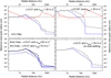 |
Fig. 11 Azimuthally averaged radial profiles of the maximum radius ar in models with different α-parameters and fragmentation velocities as indicated in the panels. The evolution time in all panels is t = 0.2 Myr. The solid blue lines are the model results, and the dashed black lines are the maximum grain radius afrag set by the fragmentation barrier defined in Eq. (26). The red solid lines show the Toomre Q-parameter calculated using Eq. (33). The red dashed lines mark the Q = 2.0 threshold for convenience. |
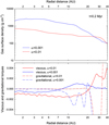 |
Fig. 12 Azimuthally averaged profiles of the gas surface density, viscous torques, and gravitational torques in the inner 40 AU in the α = 10−3 model and the α = 10−2 model (fiducial one) at t = 0.2 Myr. The torques are shown in the code units. The black dotted line marks the zero-torque line for convenience. |
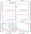 |
Fig. 13 Parameter space study of dust mass in the disk. Top and middle rows: The mass of small and grown dust in the disk (the red and blue solid lines) as a function of time for the fiducial model (top left) and for models with varying free parameters as indicated in each panel. Bottom rows: The ratio of enclosed dust masses Md,gr (r)∕Md,sm(r) as a functionof radial distance r at two evolution times: t = 0.2 Myr and t =0.4 Myr, for the fiducial model and for models with varying free parameters. |
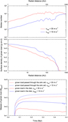 |
Fig. 14 Azimuthally averaged profiles of the Stokes number (top panel), surface density of grown dust (middle panel), and integrated masses of grown dust that passed through the sink cell and remaining in the disk (bottom panel) in models with vfrag = 10 m s−1 (blue lines) and vfrag = 30 m s−1 (red lines). The radial profiles of Σd,gr and St are taken at t = 0.2 Myr. |
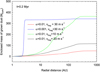 |
Fig. 15 Enclosed mass of grown dust as a function of radial distance at t = 0.2 Myr for several models with different free parameters as indicated in the legend. |
5 Model caveats and future improvements
In the current model, we did not account for the momentum transfer from dust to gas, which is frequently referred to as the dust “back reaction”. As reported in Gonzalez et al. (2017), this effect can be important if the conditions for dust trapping and subsequent growth are met. We will treat this effect in follow-up studies as soon as we find an appropriate numerical scheme to overcome the strict limitations on the hydrodynamical time step that arise when back reaction is included (see the appendix).
While the adopted model of dust growth allowed us to make a first step toward self-consistent modeling of the gas and dust dynamics during the long-term evolution of a protostellar disk, it is rather simplistic because it considers only two grain populations – small dust and grown dust. We plan to introduce more dust size bins in future studies, as was done in Birnstiel et al. (2010), for example. The assumption of a monodispersity of grown dust is hard to reconcile with the assumption of a power-law size distribution and it limits our treatment of grain collision velocities. The relative velocity is a function of size of colliding grains (Birnstiel et al. 2016), and the monodisperse approximation could underestimate the coagulation efficiency. Another critical assumption is the adoption of a constant (in time and space) power-law index of the dust size distribution. This means that at every time step, the dust particles are redistributed over a new interval in radius (amin,  ) keeping the same power-law index p. This assumption could be violated, as shown in Brauer et al. (2008), for instance. In addition, other understudied factors such as GI-induced turbulent velocity (Rice et al. 2004; Booth & Clarke 2016), grain charging (Okuzumi et al. 2011; Akimkin 2015), dependence of fragmentation velocity vfrag on the composition of dust grains, and possible temporal and spatial variations in the viscous α-parameter further complicate the picture. This diversity of important factors demands a step-by-step approach and clear understanding of the model limitations. Therefore we plan to refine the model of dust growth and complement it with a more detailed treatment of important processes in the near future.
6 Conclusions
We have numerically studied the early evolution of a circumstellar disk formed through the gravitational collapse of a rotating pre-stellar core of 1.03 M⊙. The evolution of the disk (beyond 1 AU) was computed using the numerical hydrodynamics code in the thin-disk limit that is similar in method to the ZEUS code (Stone & Norman 1992), which was modified to include a dust component. Our numerical simulations covered the embedded and early T Tauri phases of disk evolution and took the disk self-gravity (both of gas and dust), friction of gas on dust, turbulent viscosity using the α-parameterization, and stellar irradiation into account. In this study, we assumed a spatially and temporarily constant α-parameter. We followed the approach of Birnstiel et al. (2012), in which the dusty disk consists of two components: sub-micron-sized dust (≤1.0 μm), and grown dust (>1.0 μm) with a maximum radius ar calculated using the method of Stepinski & Valageas (1997). Our findings can be summarized as follows:
-
The process of dust growth known for the older protoplanetary phase also holds for the embedded phase of disk evolution. In this early phase, dust growth occurs in the entire disk, but its efficiency depends on the radial distance from the star – ar is largest in the inner disk and gradually declines with radial distance. In the inner 20–30 AU, ar is limited by the assumed fragmentation barrier, while at larger radii, ar never grows to the fragmentation barrier, implying either slowed-down dust growth or efficient inward drift of grown dust grains.
-
The process of small-to-grown dust conversion is very fast once the disk is formed. The mass of grown dust in the disk (beyond 1 AU) reaches tens or even hundreds of Earth masses as soon as in the embedded phase of star formation. The highest concentration of grown dust is found in the α = 10−3 model, where several hundred Earth masses can be accumulated in a narrow region of several AU from the star by the end of the embedded phase. Models with α = 10−2 demonstrate a notably smoother radial distribution of enclosed mass of grown dust, regardless of the chosen value for fragmentation velocity. The amount of grown dust that drifts in the inner unresolved disk regions (inside 1 AU) by the end of our simulations (0.5 Myr) can be even higher, on the order of thousands of Earth masses.
-
Dust does not usually grow to radii greater than a few centimeters. A notable exception are models with α≲10−3, where dust can grow to meter-sized boulders in the inner 10 AU. In this case, a narrow region of several AU develops in the innerdisk, which is characterized by reduced efficiency of mass transport via viscous and gravitational torques (low α and high Toomre Q-parameter). This region is similar to a classic dead zone caused exclusively by varying viscous α-parameter, and it assists dust accumulation and growth in the accompanying pressure maxima.
-
The efficiency of small-to-grown dust conversion depends on the α-parameter and fragmentation velocity vfrag. In the fiducial model (α = 10−2 and vfrag = 30 m s−1), small grains vastly dominate the dust disk mass beyond 1.0 AU. This is a consequence of efficient inward drift of grown dust in the inner unresolved disk regions (<1 AU) and continuing replenishment of small dust from the infalling envelope. For lower α, grown grains dominate in the inner several AU, where a zone with reduced mass transport develops and grown dust accumulates. For lower vfrag, the conversion is also more efficient because of a slower radial drift of grown dust grains that is due to smaller ar and lower St, meaning a better retention of grown dust in the disk, and because of the inverse dependence of the dust growth rate S(ar) on ar in our dust growth model. For vfrag = 10 m s−1, essentially all small dust (≤1.0 μm) is converted into grown dust in the inner 10 AU, in agreement with Birnstiel et al. (2010).
-
The efficiency of grown dust accumulation in spiral arms depends on the radial position in the disk and is most efficient near corotation, where the azimuthal velocity of dust grains is closest to the local velocity of the spiral pattern. This is also the region where the ratio ζ of the dust drift velocity to the dust azimuthal velocity in the local frame of reference of the spiral pattern is highest. For instance, the contrast in Σd,gr between the spiral arms and the inter-arm regions near corotation (r = 80 AU) is a factor of 2 higher than that of Σd,sm, indicating grown dust accumulation. Conversely, the inner parts of the spiral arms that are located inside corotation (r≲50 AU) are characterized by moderate pressure maxima and ζ that drops sharply, so that a clear dust concentration does not have time to form.
The results of our study demonstrate that the evolution of dust in early embedded disks needs to be taken into account when setting the initial state for dust in older protoplanetary disk studies. An upper limit on the dust radius of 0.25–1.0 μm usually taken for the MRN dust distribution (Mathis et al. 1977) is certainly exceeded by the end of the embedded phase. Moreover, the maximum radius of dust grains depends on the radial position in the disk and is not a constant in space. The radial distribution of grown dust does not follow that of small dust because of the efficient inward radial drift taking place in the embedded phase. Grown dust is more abundant in the inner than in the outer disk regions, and an appreciable amount of grown dust drifts in the inner unresolved 1 AU of the disk, probably making these disk regions more optically thick. In Appendix A, we provide analytical fits to the disk state at the end of the embedded phase.
We also note that in our models the spiral pattern in the early embedded phase of disk evolution appears to be volatile; its shape is stirred on timescales of a few thousand years by differential rotation, nonlinear interaction between different spiral modes and gravitational interaction with migrating gaseous clumps. The process of dust accumulation in spiral arms should be more efficient in the presence of a grand-design, two-arm spiral pattern as was observed in Elias 2–27 (Pérez et al. 2016; Tomida et al. 2017), given that these structures live much longer than what was found in our simulations.
Acknowledgements
We are grateful to the anonymous referee for a very insightful report that helped us to improve the manuscript and stimulated future work on dust growth models. This work was supported by the Russian Science Foundation grant 17-12-01168. The simulations were performed on the Vienna Scientific Cluster (VSC-2 and VSC-3).
Appendix A: Analytical fits to the disk at the end of the embedded phase
In this section, we provide analytical fits to the disk in the fiducial model at the end of the embedded phase at t = 0.2 Myr (see Fig. 9). These azimuthally averaged profiles can be used as an initial state when modeling older protoplanetary disks. The inner and outer disk radii are taken to be 1 AU and 300 AU, respectively.
![Mathematical equation: \begin{align} &\overline{{\mathrm{\Sigma}}}_{\textrm{g}} \, \left[{\mathrm{g} \over \mathrm{cm}^{2}}\right] =10^{2.92}\, \left({r \over \mathrm{AU}}\right)^{-0.41}, \,\,\, \mathrm{for} \,\, r < 30~\mathrm{AU}, \\ &\overline{{\mathrm{\Sigma}}}_{\textrm{g}} \, \left[{\mathrm{g} \over \mathrm{cm}^{2}}\right] =10^{5.65}\, \left( {r \over \mathrm{AU}} \right)^{-2.27}, \,\,\, \mathrm{for} \,\, r\ge 30~\mathrm{AU},\\ &\overline{{\mathrm{\Sigma}}}_{\textrm{d},\textrm{sm}} \, \left[{\mathrm{g} \over \mathrm{cm}^{2}}\right] =10^{0.67}\, \left({r \over \mathrm{AU}}\right)^{-0.28}, \,\,\, \mathrm{for} \,\, r < 30~\mathrm{AU}, \\ &\overline{{\mathrm{\Sigma}}}_{\textrm{s,sm}} \, \left[{\mathrm{g} \over \mathrm{cm}^{2}}\right] =10^{3.51}\, \left( {r \over \mathrm{AU}} \right)^{-2.23}, \,\,\, \mathrm{for} \,\, r\ge 30~\mathrm{AU},\\ &\overline{{\mathrm{\Sigma}}}_{\textrm{d},\textrm{gr}} \, \left[{\mathrm{g} \over \mathrm{cm}^{2}}\right] =10^{0.9}\, \left({r \over \mathrm{AU}}\right)^{-1.56}, \,\,\, \mathrm{for} \,\, r\ge 1.0~\mathrm{AU}\\ &\overline{a}_{\textrm{r}} \, \left[\mathrm{cm}\right] =10^{0.084}\, \left({r \over \mathrm{AU}}\right)^{0.41}, \,\,\, \mathrm{for} \,\, r < 30~\mathrm{AU}, \\ &\overline{a}_{\textrm{r}} \, \left[\mathrm{cm}\right] =10^{4.27}\, \left( {r \over \mathrm{AU}} \right)^{-2.42}, \,\,\, \mathrm{for} \,\, r\ge 30~\mathrm{AU},\\ &\overline{H}_{\textrm{g}} \, \left[\mathrm{cm}\right] =10^{-0.95}\, \left({r \over \mathrm{AU}}\right)^{1.0}, \,\,\, \mathrm{for} \,\, r < 30~\mathrm{AU}, \\ &\overline{H}_{\textrm{g}} \, \left[\mathrm{cm}\right] =10^{-1.8}\, \left( {r \over \mathrm{AU}} \right)^{1.46}, \,\,\, \mathrm{for} \,\, r\ge 30~\mathrm{AU},\\ &\overline{H}_{\textrm{d}} \, \left[\mathrm{cm}\right] =10^{-1.18}\, \left({r \over \mathrm{AU}}\right)^{0.76}, \,\,\, \mathrm{for} \,\, r < 30~\mathrm{AU}, \\ &\overline{H}_{\textrm{d}} \, \left[\mathrm{cm}\right] =10^{-2.5}\, \left( {r \over \mathrm{AU}} \right)^{1.52}, \,\,\, \mathrm{for} \,\, r\ge 30~\mathrm{AU}. \end{align}](/articles/aa/full_html/2018/06/aa31690-17/aa31690-17-eq78.png)
The scale heights of gas and grown dust (including settling) are provided so that the volume distributions of gas and dust density can be recovered.
Appendix B: Testing dust dynamics equations
Here, we provide the results of several essential test problems addressing the ability of our scheme to reproduce the known analytic solutions for a mixture of gas and dust components. While the Sod shock tube and dusty wave problems imply constant-size grains, the dust ring problem for constant Stokes numbers allows implicitly for radial variations in the dust size, as can be expected from radially varying disk densities, temperatures, and angular frequencies (see the definition of the Stokes number in Eq. (25)).
B.1:
Dust ring
For the first test problem, we consider radial drift of dust particles in a steady-state circumstellar disk. We make use of the analytic solution provided in Nakagawa et al. (1986) and Armitage (2014), for instance,
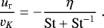 (B.1)
(B.1)
The initial radial velocity of dust is set to zero (ur = 0) and the rotation velocity is set to the Keplerian velocity (uϕ = vK). The mass of the central star is set to M* = 0.5 M⊙.
First, we use test dust particles to compare the resulting drift velocity ur with the analytical expectations. We choose  and place our particles at an initial location of r0 = 20 AU. We allow particles to drift according to the equations:
 (B.2)
(B.2)
with tstop fixed with the integration time for each particle. The drift velocities are measured when dust particles reach a distance of 10 AU. The results for different Stokes parameters are shown in Fig. B.1. Clearly, our numerical scheme reproduces the expected analytical solution for both small and large Stokes numbers well.
 |
Fig. B.1 Radial velocity of test particles in terms of Keplerian velocity. The points indicate the results of numerical simulations, and the solid line expresses the analytical solution (B.1). |
In the second step, we test the ability of our numerical hydrodynamics code to transport a dust ring across the disk. We set a dust ring with a unit surface density and a width of 10 AU located initially between 50 AU and 60 AU. We set  and compute the dynamics of the dust ring for different values of the Stokes number. We keep the Stokes parameter fixed in space and time during the integration. The results are shown in Fig. B.2 for runs with St = 10−3, St = 10−1, St = 0.5, and St = 0.9. The black dashed lines outline the initial shape and position of the dust ring, and the solid blue lines outline the ring after it drifted toward the star by more than its full width. The vertical dash-dotted lines present the analytic solutions for the edges of the ring (see, e.g., Stoyanovskaya et al. 2017):
![Mathematical equation: \begin{equation*}r^{3/2}=r_0^{3/2}-\frac{3 \sqrt[]{GM \ast} \eta t}{2 (\textrm{St}+\textrm{St}^{-1})}. \end{equation*}](/articles/aa/full_html/2018/06/aa31690-17/aa31690-17-eq83.png) (B.3)
(B.3)
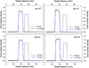 |
Fig. B.2 Inward drift of a dust ring. The black dashed lines show the initial position of the ring, while the blue solid lines outline the position and shape of the ring after it drifted inward by more than its full width. The vertical dash-dotted lines present the analytic solutions for the edges of the ring. |
Evidently, the position of the ring is reproduced rather well for all Stokes numbers that are pertinent to our modeling. The edges of the ring are smeared over several grid zones, which is consistent with the accuracy of our advection scheme. We note that the peak value of the ring increases as it drifts inward because of the shrinking surface area of the ring.
Sod shock tube
This test is often used to assess the ability of a numerical algorithm to accurately track the position of moderate shock waves and contact discontinuities. Initial conditions involve two discontinuous states along the z-axis, with a hot dense gas on the left and cold rarified gas on the right. More specifically, we set the pressure and density of gas at z ∈ [0, 0.5] to 1.0, while at z ∈ [0.5, 1.0], the gas pressure is 0.1 and the gas density is 0.125. The velocity of a γ = 1.4 gas is initially zero everywhere. The dust component has the same initial distribution as that of gas, but the dust pressure is set to zero. The dust-to-gas ratio is therefore equal to unity everywhere.
The analytic solution for the gas and dust mixture is only known in the limit of short stopping times compared to the time of shock wave propagation. We use the SPLASH code (Price 2007) to generate the analyticsolution (on its stationary stage) with a modified sound speed for the gas-dust medium cd (see Sect. 3). In this case, the dust velocity is believed to be equal to the gas velocity, when the density of the dust is equal to the density of the gas multiplied by the initial dust-to-gas ratio. We follow the terminology of Laibe & Price (2012) and introduce the drag parameter K, and we define the stopping time as tstop = ρgas∕K, where ρgas = 1 is the gas density in the left half of the shock tube. For this test problem, we also included the back reaction of dust onto gas by adding the corresponding term to the gas dynamics equation. Figure B.3 presents the test results for K = 1000. The first and second rows present the resulting gasdistributions at t = 0.24, while the bottom row shows those of dust. The numerical resolution is 200 grid zones and the artificial viscosity parameter is set to C2 = 2, implying that shocks are spread over two grid zones.
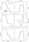 |
Fig. B.3 Sod shock tube problem in the limit of a short stopping time and taking the back reaction of dust on gas into account. The top and middle rows of panels present solutions for the gas component, while the bottom rows show solutions for the dust component. The black solid line shows the analytic solution, and the color lines present numerical solutions for different values of the time step as indicated in the top left panel. |
We have found that in order to achieve a reasonable agreement with the analytic solution, one needs a time step d t that is much smaller than the stopping time. For instance, the blue lines present the test results for d t = tstop, which obviously show considerable deviations from the analytic solution, but the green lines corresponding to d t = 0.05tstop match the analytic solution much better (still, some deviations, particularly in the specific energy, are notable). Similar results were obtained for K = 100.
This problem with the numerical scheme is analogous to that highlighted in Laibe & Price (2012), but they formulated it in terms of spatial resolution, while we think it is better to express it in terms of the time step and stopping time. The time step is directly linked to the numerical resolution for explicit numerical hydrodynamics solvers, such as our own, so the two approaches are similar.
Our test essentially demonstrates that for a medium with a high concentration of dust particles that are strongly coupled to the gas, the stopping time has to be resolved by at least 50 time steps to adequately track shock waves that can be present in GI unstable disks.
Fortunately, we have found that our scheme works much better if the back reaction of the dust component on the gas is neglected (as we did in the present study). Figure B.4 presents the corresponding results for the dust-to-gas ratio of 0.01 when the reaction of dust on the gas component has a small effect and can be neglected. The red lines provide the analytic solution at t = 0.24, while the filled circles are the numerical solution. The time step in this case is similar to the stopping time. Evidently, the code reproduces the analytic solution in both gas and dust quite well. Similar results were obtained for d t = 2tstop by decreasing the numerical resolution by a factor of 2. We cannot test the scheme for even larger time steps because of the Courant limitation on the time step, but this test already demonstrates that if the back reaction of dust on gas can be neglected, then there is no need to introduce another very stiff limitation on the time step to resolve the stopping time by at least 50 time steps. B.3:
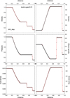 |
Fig. B.4 Sod shock tube problem in the limit of a short stopping time, but without taking the back reaction of dust on gas into account. The top and middle rows of panels present solutions for the gas component, while the bottom rows show solutions for the dust component. The red lines present the analytical solution, and the filled circles are the numerical solution for the time step similar to the stopping time. |
Dusty wave
The dusty wave problem tests the propagation of linear waves in the mixture of gas and dust. Unlike the Sod shock tube problem, where the analytical solution for the weak coupling between gas and dust (low drag parameter K) is not known, the dusty wave problem has analytical solutions for both weak and strong coupling. In particular, this test allows us to estimate theaccuracy with which gas densities and gas and dust velocities are calculated during the propagating and damping of acoustic waves.
The initial setup consists of a sinusoidal wave of the form
 (B.4)
(B.4)
 (B.5)
(B.5)
We adopt isothermal gas with cs=1,  , k = 1, and δ = 0.01 throughout this section and vary K and
  . All simulations were made with 100 grid zones on unit distance with artificial viscosity parameter C2 = 2 and periodic boundary conditions. The analytical solution is given in Laibe & Price (2011); we used the code accompanying their paper.
Figure B.5 presents the gas and dust velocities at t = 0.5 for K = 1000. The dust-to-gas ratio is  . As in Appendix sectionlinking B.2, we varied the time step from 0.05tstop to tstop. Clearly, thenumerical solution differs notably from the analytical one for d t = tstop, but decreasing the time step to dt = 0.05tstop enables us to achieve a reasonably good agreement with the analytical solution for both the gas and dust velocities. We note that for lower dust-to-gas ratios, the requirement on the time step is less strict. Figure B.6 presents the gas and dust velocities for the same time instance t = 0.5 obtained forK = 100 and d2g = 0.011. For dt = tstop, the agreement between the numerical and analytical solution is much better than for the case of d2g = 1.0, but the dust velocity is calculated less accurately than the gas velocity.
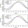 |
Fig. B.5 Solution of the dusty wave problem for a strong coupling between gas and dust (K = 1000) and a dust-to-gas ratio d2g = 1 at a time instance t = 0.5. The top panel shows the gas velocity, while the bottom panel shows the dust velocity. The color lines present numerical solutions obtained with different time steps d t, while the black line shows the analytical solution. |
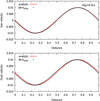 |
Fig. B.6 Solution of the dusty wave problem for a strong coupling between gas and dust (K = 100) and a dust-to-gas ratio d2g = 0.011 at a time t = 0.5. The top panel shows the gas velocity, while the bottom panel shows the dust velocity. The black dots present numerical solutions obtained with the time step d t = tstop, while the red line shows the analytical solution. |
Finally, we consider the dusty wave with a weak coupling between the gas and dust, K = 1. As was demonstrated earlier, the case of comparable dust and gas densities is most challenging for simulations. We therefore choose d2g = 1.0 for this testrun. The time step was defined by the Courant condition with a limiter C = 0.5. The resulting gas and dust velocities are shown in Fig. B.7 for different time instances. Clearly, our scheme performs well for the case of weak coupling between the gas and dust even when back reaction is taken into account.
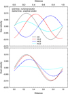 |
Fig. B.7 Solution of the dusty wave problem for a weak coupling between gas and dust (K = 1) and a dust-to-gas ratio d2g = 1 at times t = 0, 0.2, 0.5, and 2.0. The top panel shows the gas velocity, while the bottom panel shows the dust velocity. The solid lines present numerical solutions at different times as indicated in the legend, while the dashed lines present the corresponding analytical solutions. The two solutions are often almost indistinguishable. |
References
- Akimkin, V. V. 2015, Astron. Rep., 59, 747 [NASA ADS] [CrossRef] [Google Scholar]
- André, P., Ward-Thompson, D., & Barsony, M. 1993, ApJ, 406, 122 [NASA ADS] [CrossRef] [Google Scholar]
- Ansdell, M., Williams, J. P., van der Marel, N., Carpenter, J. M., Guidi, G., et al. 2016, ApJ, 828, 46A [NASA ADS] [CrossRef] [Google Scholar]
- Armitage, P. J. 2014, ArXiv e-prints [arXiv:astro-ph/0701485] [Google Scholar]
- Benz, W. 2000, Space Sci. Rev., 92, 279 [NASA ADS] [CrossRef] [Google Scholar]
- Birnstiel, T., Dullemond, C. P., & Brauer, F. 2010, A&A 513, A79 [NASA ADS] [CrossRef] [EDP Sciences] [Google Scholar]
- Birnstiel, T., Klahr, H., & Ercolano, B. 2012, A&A, 539, A148 [NASA ADS] [CrossRef] [EDP Sciences] [Google Scholar]
- Birnstiel, T., Fang, M., & Johansen, A. 2016, Space Sci. Rev., 205, 41 [NASA ADS] [CrossRef] [Google Scholar]
- Blum, J., & Wurm, G. 2008, ARA&A, 46, 21 [NASA ADS] [CrossRef] [EDP Sciences] [Google Scholar]
- Boley, A. C. 2009, ApJ, 695, L53 [NASA ADS] [CrossRef] [Google Scholar]
- Booth, R. A., & Clarke, C. J. 2016, MNRAS, 458, 2676 [NASA ADS] [CrossRef] [Google Scholar]
- Boss, A. P. 2001, ApJ, 563, 367 [NASA ADS] [CrossRef] [Google Scholar]
- Brauer, F., Dullemond, C. P., & Henning, T. 2008, A&A, 480, 859 [NASA ADS] [CrossRef] [EDP Sciences] [Google Scholar]
- Caselli, P., Benson, P. J., Myers, P. C., & Tafalla, M. 2002, ApJ, 572, 238 [NASA ADS] [CrossRef] [Google Scholar]
- Cha, S.-H., & Nayakshin, S. 2011, MNRAS, 415, 3319 [NASA ADS] [CrossRef] [Google Scholar]
- Colella, P., & Woodward, P. R. 1984, J. Comput. Phys., 54, 174 [NASA ADS] [CrossRef] [MathSciNet] [Google Scholar]
- Dapp, W. B., & Basu, S. 2009, MNRAS, 395, 1092 [NASA ADS] [CrossRef] [Google Scholar]
- Dominik, C., & Tielens, A. G. G. M. 1997, ApJ, 480, 647 [NASA ADS] [CrossRef] [Google Scholar]
- Dong, R., Vorobyov, E., Pavlyuchenkov, Y., Chiang, E., & Liu, H. B. 2016, ApJ, 823, 141 [NASA ADS] [CrossRef] [Google Scholar]
- Flock, M., Henning, Th., & Klahr, H. 2012, ApJ, 761, 95 [NASA ADS] [CrossRef] [Google Scholar]
- Frimann, S., Jorgensen, J. K., Dunham, M. M., et al. 2017, A&A, 602, A120 [NASA ADS] [CrossRef] [EDP Sciences] [Google Scholar]
- Gibbons, P. G., Rice, W. K. M., & Mamatsashvili, G. R. 2012, MNRAS, 426, 1444 [NASA ADS] [CrossRef] [Google Scholar]
- Gibbons, P. G., Mamatsashvili, G. R., & Rice, W. K. M 2015, MNRAS, 453, 4232 [NASA ADS] [CrossRef] [Google Scholar]
- Gonzalez, J.-F., Laibe, G., Maddison, S. T., Pinte, C., & Ménard, F. 2015, Planet. Space Sci., 116, 48 [NASA ADS] [CrossRef] [Google Scholar]
- Gonzalez, J.-F., Laibe, G., & Maddison, S. T. 2017, MNRAS, 467, 1984 [NASA ADS] [Google Scholar]
- Hubbard, A. 2017, MNRAS, 465, 1910 [Google Scholar]
- Ilee, J. D., Boley, A. C., Caselli, P. 2011, MNRAS, 417, 2950 [NASA ADS] [CrossRef] [Google Scholar]
- Ivlev, A. V., Akimkin, V. V., & Caselli, P. 2016, ApJ, 833, 92 [NASA ADS] [CrossRef] [Google Scholar]
- Jørgensen, J. K., Visser, R., Williams, J. P., & Bergin, E. A. 2015, A&A, 579, A23 [NASA ADS] [CrossRef] [EDP Sciences] [Google Scholar]
- Kimura, S. S., Kunitomo, M., & Takahashi, S. Z. 2016, MNRAS, 461, 2257 [NASA ADS] [CrossRef] [Google Scholar]
- Kornet, K., Stepinski, T. F., & Różyczka, M. 2001, A&A, 378, 180 [NASA ADS] [CrossRef] [EDP Sciences] [Google Scholar]
- Laibe, G., & Price, D. J. 2011, MNRAS, 418, 1491 [NASA ADS] [CrossRef] [Google Scholar]
- Laibe, G., & Price, D. J. 2012, MNRAS, 420, 2345 [NASA ADS] [CrossRef] [Google Scholar]
- Li, J. I.-H., Liu, H. B., Hasegawa, Y., & Hirano, N. 2017, ApJ, 840, 72 [NASA ADS] [CrossRef] [Google Scholar]
- Liu, H. B., Vorobyov, E. I., Dong, R., et al. 2017, A&A, 602, A19 [NASA ADS] [CrossRef] [EDP Sciences] [Google Scholar]
- Lodato, G., & Rice, W. K. M. 2005, MNRAS, 358, 1489 [NASA ADS] [CrossRef] [Google Scholar]
- Lynden-Bell, D., & Pringle J. E. 1974, MNRAS, 168, 603 [NASA ADS] [CrossRef] [Google Scholar]
- Masset, F. 2000, A&AS, 141, 165 [NASA ADS] [CrossRef] [EDP Sciences] [Google Scholar]
- Mathis, J. S., Rumpl, W., & Nordsieck, K. H. 1977, ApJ, 217, 425 [NASA ADS] [CrossRef] [Google Scholar]
- Mayer, L., Quinn, T., Wadsley, J., & Stadel, J. 2002, Science, 298, 1756 [NASA ADS] [CrossRef] [PubMed] [Google Scholar]
- Meyer, D. M.-A., Vorobyov, E. I., Kuiper, R. & Kley, W. 2017, MNRAS, 464, 90 [Google Scholar]
- Nakagawa, Y., Sekiya, M., & Hayashi, C. 1986, Icarus, 67, 375 [NASA ADS] [CrossRef] [Google Scholar]
- Nayakshin, S. 2010, MNRAS, 408, 36 [Google Scholar]
- Nayakshin, S. 2017, PASA, 34, e002 [NASA ADS] [CrossRef] [Google Scholar]
- Ohtani, T., Kimura, S. S., Tsuribe, T., & Vorobyov, E. I. 2014, PASJ, 66, 112 [NASA ADS] [CrossRef] [Google Scholar]
- Okuzumi, S., Tanaka, H., Takeuchi, T., & Sakagami, M. A. 2011, ApJ, 731, 95 [NASA ADS] [CrossRef] [Google Scholar]
- Ormel, C. W., & Cuzzi, J. N. 2007, A&A, 466, 413 [NASA ADS] [CrossRef] [EDP Sciences] [Google Scholar]
- Pérez, L. M., Carpenter, J. M., Andrews, S. M., et al. 2016, Science, 353, 1519 [NASA ADS] [CrossRef] [Google Scholar]
- Pinilla, P., Flock, M., de Juan Ovelar, M., & Birnstiel, T. 2016, A&A, 596, A81 [NASA ADS] [CrossRef] [EDP Sciences] [Google Scholar]
- Price, D. 2017, PASA, 24, 159 [Google Scholar]
- Rice, W. K. M., Lodato, G., Pringle, J. E., Armitage, P. J., & Bonnell, I. A. 2004, MNRAS, 355, 543 [NASA ADS] [CrossRef] [Google Scholar]
- Rice, W. K. M., Mayo, J. H., & Armitage, P. J. 2010, MNRAS, 402, 1740 [NASA ADS] [CrossRef] [Google Scholar]
- Semenov, D., Henning, T., Helling, C., Ilgner, M., & Sedlmayr, E. 2003, A&A, 410, 611 [NASA ADS] [CrossRef] [EDP Sciences] [Google Scholar]
- Shakura, N. I., & Sunyaev, R. A. 1973, A&A, 24, 337 [NASA ADS] [Google Scholar]
- Simon, J. B., Lesur, G., Kunz, M. W., & Armitage, P. J. 2015, ApJ, 454, 1117 [Google Scholar]
- Sirono, S., & Ueno, H. 2014, 40th COSPAR Scientific Assembly, 40, B0.5-2-14 [Google Scholar]
- Stamatellos, D. 2015, ApJ, 810, L11 [NASA ADS] [CrossRef] [Google Scholar]
- Stamatellos, D., Whitworth, A. P., & Hubber, D. A. 2012, MNRAS, 427, 1182 [NASA ADS] [CrossRef] [Google Scholar]
- Stepinski, T. F., & Valageas, P. 1997, A&A, 319, 1007 [NASA ADS] [Google Scholar]
- Stone, J. M., & Norman, M. L. 1992, ApJS, 80, 753 [Google Scholar]
- Stoyanovskaya, O. P., Snytnikov, V. N., & Vorobyov, E. I. 2017, Astron. Rep., 61, 1044 [NASA ADS] [CrossRef] [Google Scholar]
- Tomida, K., Machida, M. N., Hosokawa, T. Sakurai, Y., & Lin, C. H. 2017, ApJ, 835, L11 [NASA ADS] [CrossRef] [Google Scholar]
- Turner, N. J., Fromang, S., Gammie, C., et al. 2014, Protostars and Planets VI (Tucson, AZ: Univ. Arizona Press), 411 [Google Scholar]
- Visser, R., & Dullemond, C. P. 2010, A&A, 519, A28 [NASA ADS] [CrossRef] [EDP Sciences] [Google Scholar]
- Vorobyov, E. I. 2010, ApJ, 723, 1294 [NASA ADS] [CrossRef] [Google Scholar]
- Vorobyov, E. I. 2013, A&A, 552, A129 [NASA ADS] [CrossRef] [EDP Sciences] [Google Scholar]
- Vorobyov, E. I., & Basu, S. 2006, ApJ, 650, 956 [NASA ADS] [CrossRef] [Google Scholar]
- Vorobyov, E. I., & Basu, S. 2007, MNRAS, 381, 1009 [NASA ADS] [CrossRef] [Google Scholar]
- Vorobyov, E. I., & Basu, S. 2009, MNRAS, 393, 822 [NASA ADS] [CrossRef] [Google Scholar]
- Vorobyov, E. I., & Basu, S. 2010, ApJ, 719, 1896 [NASA ADS] [CrossRef] [Google Scholar]
- Vorobyov, E. I., & Basu, S. 2015, ApJ, 805, 115 [NASA ADS] [CrossRef] [Google Scholar]
- Vorobyov E. I., Baraffe I., Harries T. & Chabrier G., et al. 2013, A&A, 557, A35 [NASA ADS] [CrossRef] [EDP Sciences] [Google Scholar]
- Vorobyov, E. I., Elbakyan, V., Hosokawa, T., et al. 2017, A&A, 605, A77 [NASA ADS] [CrossRef] [EDP Sciences] [Google Scholar]
- Williams, J. P. & Best, W. M. J. 2014, ApJ, 788, 59 [NASA ADS] [CrossRef] [Google Scholar]
- Wada, K., Tanaka, H., Suyama, T., Kimura, H., & Yamamoto, T. 2009, ApJ, 702, 1490 [NASA ADS] [CrossRef] [Google Scholar]
- Yorke, H. W., & Bodenheimer, P., 2008, in Massive Star Formation: Observations Confront Theory, eds. H. Beuther, H. Linz, & T. Henning (San Francisco: ASP), ASP Conf. Ser., 387, 189 [NASA ADS] [Google Scholar]
- Zhu, Z., Hartmann, Lee, Gammie, C., & McKinney, J. C. 2009, ApJ, 701, 620 [NASA ADS] [CrossRef] [Google Scholar]
- Zhu, Z., Nelson, R. P., Dong, R., Espaillat, C., & Hartmann, L. 2012, ApJ, 755, 6 [NASA ADS] [CrossRef] [Google Scholar]
All Figures
|
Fig. 1 Illustration of the adopted scheme for dust growth. The size distributions of dust grains at the current
n
and next n + 1 time steps are shown with the red and blue lines, respectively. Here, amin
is the minimum radius of small dust grains, while |
| In the text | |
|
Fig. 2 Schematic illustration of the inner boundary condition. The mass of material Δ Mflow that passes through the sink cell from the active inner disk is further divided into two parts: the mass Δ M* contributing to the growing central star, and the mass ΔMs.c. settling in the sink cell. |
| In the text | |
|
Fig. 3 Gas surface density distribution in the inner 1000 × 1000 AU2 box at six evolutionary times starting from the onset of gravitational collapse. The inset shows the fragments formed in the disk via gravitational fragmentation. The black line in the inset highlights the region where the Toomre parameter is less than unity. The scale bar is in log g cm−2. |
| In the text | |
|
Fig. 4 Zoom-in onto the inner disk regions at t = 0.2 Myr: left column –200 × 200 AU2, middle column – 60 × 60 AU2, and right column – 10 × 10 AU2. Shown are the gas surface density in log g cm−2 (top row), grown dust surface density in log g cm−2 (second row), gas-to-grown dust mass ratio in log scale (third row), Stokes number in log scale (fourth row), and maximum radius of dust grains ar in log cm. The contour lines in the third, fourth, and fifth rows delineate the spiral pattern in the gas surface density for convenience. |
| In the text | |
|
Fig. 5 Velocity field for grown dust (relative to the gas) superimposed on the gas surface density map in the vicinity of a prominent spiral arm at t = 0.2 Myr. |
| In the text | |
|
Fig. 6 Surface densities of gas (red solid lines), small dust (blue dashed lines), and grown dust (black solid lines) taken along the azimuthal cuts at different distances from the star: r = 20 AU, r = 50 AU, r = 82 AU, and r = 150 AU. The dashed pink and solid cyan lines show the gas pressure (in the code units) and the maximum radius of dust grains ar (in cm) taken along the same cuts. The evolution time is t = 0.2 Myr. We applied different scaling factors for the small dust density, grown dust density, and maximum dust radius. |
| In the text | |
|
Fig. 7 Radial profiles of the azimuthal component of the dust drift velocity |uϕ,drift|, the azimuthal component of the dust bulk velocity relative to the local velocity of the spiral pattern uϕ − vsp, their ratio ζ = |uϕ,drift|∕|uϕ − vsp|, and the parameter η. |
| In the text | |
|
Fig. 8 Surface density of grown dust, maximum radius of dust grains, and Stokes number as a function of the gas surface density within 200 AU from the star at t = 0.2 Myr. The black solid lines illustrate the linear and quadratic dependencies to facilitate comparison. |
| In the text | |
|
Fig. 9 Azimuthally averaged radial profiles of the gas surface density (blue solid lines, top row), gas midplane temperature (blue solid lines, second row), surface densities of small and grown dust (blue dashed and solid lines, third row), and maximum radius of grown dust (blue lines, bottom row) at two evolutionary times: t = 0.2 Myr (left column) and t = 0.4 Myr (right column). The dotted lines present various dependencies on radial distance r to facilitate comparison. The black dashed and dash-dotted lines in the second row show the gas midplane temperatures that would be expected in the presence of either stellar + background irradiation or viscous heating only, respectively. The red dash-dotted lines in the third row are the total dust-to-gas mass ratio. Finally, the black dashed lines in the bottom row present the fragmentation barrier. |
| In the text | |
|
Fig. 10 Toppanel: integrated masses of the disk and envelope (solid and dash-dotted line) and the mass of the central star (dashed line) as a function of time. Bottom panel: total masses of the grown dust (blue solid line) and small dust (red solid line) in the disk as a function of time. We also show the masses of small and grown dust that passed through the sink cell (red dashed and blue dashed lines, respectively). |
| In the text | |
|
Fig. 11 Azimuthally averaged radial profiles of the maximum radius ar in models with different α-parameters and fragmentation velocities as indicated in the panels. The evolution time in all panels is t = 0.2 Myr. The solid blue lines are the model results, and the dashed black lines are the maximum grain radius afrag set by the fragmentation barrier defined in Eq. (26). The red solid lines show the Toomre Q-parameter calculated using Eq. (33). The red dashed lines mark the Q = 2.0 threshold for convenience. |
| In the text | |
|
Fig. 12 Azimuthally averaged profiles of the gas surface density, viscous torques, and gravitational torques in the inner 40 AU in the α = 10−3 model and the α = 10−2 model (fiducial one) at t = 0.2 Myr. The torques are shown in the code units. The black dotted line marks the zero-torque line for convenience. |
| In the text | |
|
Fig. 13 Parameter space study of dust mass in the disk. Top and middle rows: The mass of small and grown dust in the disk (the red and blue solid lines) as a function of time for the fiducial model (top left) and for models with varying free parameters as indicated in each panel. Bottom rows: The ratio of enclosed dust masses Md,gr (r)∕Md,sm(r) as a functionof radial distance r at two evolution times: t = 0.2 Myr and t =0.4 Myr, for the fiducial model and for models with varying free parameters. |
| In the text | |
|
Fig. 14 Azimuthally averaged profiles of the Stokes number (top panel), surface density of grown dust (middle panel), and integrated masses of grown dust that passed through the sink cell and remaining in the disk (bottom panel) in models with vfrag = 10 m s−1 (blue lines) and vfrag = 30 m s−1 (red lines). The radial profiles of Σd,gr and St are taken at t = 0.2 Myr. |
| In the text | |
|
Fig. 15 Enclosed mass of grown dust as a function of radial distance at t = 0.2 Myr for several models with different free parameters as indicated in the legend. |
| In the text | |
|
Fig. B.1 Radial velocity of test particles in terms of Keplerian velocity. The points indicate the results of numerical simulations, and the solid line expresses the analytical solution (B.1). |
| In the text | |
|
Fig. B.2 Inward drift of a dust ring. The black dashed lines show the initial position of the ring, while the blue solid lines outline the position and shape of the ring after it drifted inward by more than its full width. The vertical dash-dotted lines present the analytic solutions for the edges of the ring. |
| In the text | |
|
Fig. B.3 Sod shock tube problem in the limit of a short stopping time and taking the back reaction of dust on gas into account. The top and middle rows of panels present solutions for the gas component, while the bottom rows show solutions for the dust component. The black solid line shows the analytic solution, and the color lines present numerical solutions for different values of the time step as indicated in the top left panel. |
| In the text | |
|
Fig. B.4 Sod shock tube problem in the limit of a short stopping time, but without taking the back reaction of dust on gas into account. The top and middle rows of panels present solutions for the gas component, while the bottom rows show solutions for the dust component. The red lines present the analytical solution, and the filled circles are the numerical solution for the time step similar to the stopping time. |
| In the text | |
|
Fig. B.5 Solution of the dusty wave problem for a strong coupling between gas and dust (K = 1000) and a dust-to-gas ratio d2g = 1 at a time instance t = 0.5. The top panel shows the gas velocity, while the bottom panel shows the dust velocity. The color lines present numerical solutions obtained with different time steps d t, while the black line shows the analytical solution. |
| In the text | |
|
Fig. B.6 Solution of the dusty wave problem for a strong coupling between gas and dust (K = 100) and a dust-to-gas ratio d2g = 0.011 at a time t = 0.5. The top panel shows the gas velocity, while the bottom panel shows the dust velocity. The black dots present numerical solutions obtained with the time step d t = tstop, while the red line shows the analytical solution. |
| In the text | |
|
Fig. B.7 Solution of the dusty wave problem for a weak coupling between gas and dust (K = 1) and a dust-to-gas ratio d2g = 1 at times t = 0, 0.2, 0.5, and 2.0. The top panel shows the gas velocity, while the bottom panel shows the dust velocity. The solid lines present numerical solutions at different times as indicated in the legend, while the dashed lines present the corresponding analytical solutions. The two solutions are often almost indistinguishable. |
| In the text | |
Current usage metrics show cumulative count of Article Views (full-text article views including HTML views, PDF and ePub downloads, according to the available data) and Abstracts Views on Vision4Press platform.
Data correspond to usage on the plateform after 2015. The current usage metrics is available 48-96 hours after online publication and is updated daily on week days.
Initial download of the metrics may take a while.