| Issue |
A&A
Volume 614, June 2018
|
|
|---|---|---|
| Article Number | A8 | |
| Number of page(s) | 22 | |
| Section | Cosmology (including clusters of galaxies) | |
| DOI | https://doi.org/10.1051/0004-6361/201731433 | |
| Published online | 06 June 2018 | |
MACS J0416.1–2403: Impact of line-of-sight structures on strong gravitational lensing modelling of galaxy clusters
1
Max-Planck-Institut für Astrophysik,
Karl-Schwarzschild Str. 1,
85741
Garching, Germany
e-mail: This email address is being protected from spambots. You need JavaScript enabled to view it.
2
Institute of Astronomy and Astrophysics, Academia Sinica,
23-141,
Taipei
10617, Taiwan
3
Physik-Department, Technische Universität München,
James-Franck-Straße 1,
85748
Garching, Germany
4
Dipartimento di Fisica, Università degli Studi di Milano,
via Celoria 16,
20133
Milano, Italy
5
Dark Cosmology Centre, Niels Bohr Institute, University of Copenhagen,
Juliane Maries Vej 30,
2100
Copenhagen, Denmark
6
University Observatory Munich,
Scheinerstrasse 1,
81679
Munich, Germany
7
INAF – Osservatorio Astronomico di Trieste,
via G. B. Tiepolo 11,
34143
Trieste, Italy
8
Dipartimento di Fisica e Scienze della Terra, Università degli Studi di Ferrara,
via Saragat 1,
44122
Ferrara, Italy
9
Osservatorio di Bologna INAF – Osservatorio Astronomico di Bologna,
via Ranzani 1,
40127
Bologna, Italy
10
INAF – Osservatorio Astronomico di Capodimonte,
via Moiariello 16,
80131
Napoli, Italy
11
Pyörrekuja 5 A,
04300
Tuusula, Finland
Received:
23
June
2017
Accepted:
11
December
2017
Abstract
Exploiting the powerful tool of strong gravitational lensing by galaxy clusters to study the highest-redshift Universe and cluster mass distributions relies on precise lens mass modelling. In this work, we aim to present the first attempt at modelling line-of-sight (LOS) mass distribution in addition to that of the cluster, extending previous modelling techniques that assume mass distributions to be on a single lens plane. We have focussed on the Hubble Frontier Field cluster MACS J0416.1–2403, and our multi-plane model reproduces the observed image positions with a rms offset of ~0.′′53. Starting from this best-fitting model, we simulated a mock cluster that resembles MACS J0416.1–2403 in order to explore the effects of LOS structures on cluster mass modelling. By systematically analysing the mock cluster under different model assumptions, we find that neglecting the lensing environment has a significant impact on the reconstruction of image positions (rms ~0.′′3); accounting for LOS galaxies as if they were at the cluster redshift can partially reduce this offset. Moreover, foreground galaxies are more important to include into the model than the background ones. While the magnification factor of the lensed multiple images are recovered within ~10% for ~95% of them, those ~5% that lie near critical curves can be significantly affected by the exclusion of the lensing environment in the models. In addition, LOS galaxies cannot explain the apparent discrepancy in the properties of massive sub-halos between MACS J0416.1–2403 and N-body simulated clusters. Since our model of MACS J0416.1–2403 with LOS galaxies only reduced modestly the rms offset in the image positions, we conclude that additional complexities would be needed in future models of MACS J0416.1–2403.
Key words: gravitational lensing: strong / galaxies: clusters: general / galaxies: clusters: individual: MACS J0416.1–2403 / dark matter
© ESO 2018
1 Introduction
Massive galaxy clusters are the largest gravitationally bound structures in the Universe and they are located at the nodes of the cosmic web. According to the currently accepted cosmological model, which consists of a cold dark matter dominated Universe with a cosmological constant (ΛCDM), more massive structures form by accretion and assembly of smaller self-bound individual systems (e.g. Springel et al. 2006). As such, galaxy clusters are not only a perfect laboratory to study the formation and evolution of structures in the Universe (e.g. Dressler 1984; Kravtsov & Borgani 2012, and references therein), but also to study the mass-energy density components, such as dark matter and dark energy, and to constrain cosmological parameters (e.g. Jullo et al. 2010; Caminha et al. 2017; Rozo et al. 2010; Planck Collaboration XX 2014, among others).
They are also very efficient cosmic telescopes. Indeed, the magnification effect produced by gravitational lensing with galaxy clusters provides a powerful tool to detect and study high-redshift galaxies, that would be undetectable with currently available instruments. Gravitational lensing is a relativistic effect for which the light travelling from a source towards the observer is bent by the presence of matter in-between. Consequently, the source is observed at a different position than it actually is, distorted in shape, and in some cases also multiply imaged (in the so-called strong lensing regime). It also appears magnified by a factor μ (magnification). Once the magnification μ is known, due to surface brightness conservation, the intrinsic brightness and shape of the source galaxy can be reconstructed. This allows study of high-redshift galaxies, providing crucial probes of structure formation and galaxy evolution.
In the past decades, gravitational lensing with clusters has highly improved our knowledge of the mass distribution in clusters, and has led to the discovery of some of the highest-redshift galaxies (e.g. Coe et al. 2013; Bouwens et al. 2014). Being such versatile laboratories for many studies, galaxy clusters have been searched for and studied in depth in recent years. In particular, the Hubble Frontier Fields initiative (HFF; P.I.: J. Lotz) has exploited the Hubble Space Telescope (HST) sensitivity and the magnification effect of six targeted strong lensing clusters to detect the high-redshift Universe. These six clusters were observed in seven optical and near-IR bands using the Advanced Camera for Survey (ACS) and the Wide Field Camera 3 (WFC3), achieving an unprecedent depth of ~ 29 mag (AB). The HFF initiative has provided a sample of high-redshift galaxies that will allow one to investigate their properties in a statistically significant way.
As previously mentioned, to reconstruct the intrinsic brightness of these far away sources, the magnification effect needs to be accounted for. This can be done only by modelling in detail the mass distribution of the lensing cluster. High precision reconstruction of cluster lenses is necessary to avoid systematic errors affecting the cluster mass reconstruction or the source brightness substantially. In recent years, the models of clusters of galaxies have been performed with increasing precision (e.g. Grillo et al. 2015; Caminha et al. 2017, among others). However, current analyses using single-plane approach seem to have reached a limit in reproducing the observables. This approach consists of modelling the lens as if it were an isolated system on a single redshift-plane, and has led to models with an rms between theobserved and predicted positions of the multiple images of the strongly lensed background sources of ~ 0.′′ 5–1″, which is greater than the observational uncertainty (~0.′′05). To account for the residual offset, it might be necessary to also consider the lensing environment in the model. In fact, we expect that the contribution of the line-of-sight (LOS) matter can affect the observables more than the observational uncertainties. Therefore, this effect needs to be taken into account to study its contribution to the recovered offset between observations and current cluster models (e.g. D’Aloisio et al. 2014; Caminha et al. 2016).
In this work we have simulated galaxy cluster lensing observations, accounting for the LOS effects using multi-plane lensing formalism, and study the effects of the LOS structures on the magnification and position of the images. We then analysed these simulated data to study the cluster mass distribution and to reconstruct the high-redshift galaxies’ intrinsic brightness. We analysed toy models of clusters, and then a mock model that is as similar as possible to the HFF cluster MACS J0416.1–2403, to make our study more realistic.
The work is organised as follows: in Sect. 2 we describe our analysis’ method, the multi-plane formalism, and the profiles we use to parametrise the lens cluster. In Sect. 3 we analyse toy models of simplistic clusters and in Sect. 4 we present our model of the mass distribution of a real cluster, namely the HFF cluster MACS J0416.1–2403. We used our best-fit model to generate lensing observables from a simulated mock system that mimics MACS J0416.1–2403 and we model the simulated cluster with different assumptions. We discuss our results in Sect. 5.
Throughout this work, we have assumed a flat Λ-CDM cosmology with H0 = 70 km s−1 Mpc^-1 and Ω Λ = 1 −ΩM = 0.70. From the redshift of the lens (zc = 0.396) in Sect. 4.1, one arcsecond at the lens plane in MACS J0416.1–2403 corresponds to ~ 5.34 kpc. The magnitudes are all given in the AB system. The uncertainty we have considered for all the image positions corresponds to the pixel scale 0.′′065, unless stated otherwise.
2 Multiple lens plane modelling
In this work, the modelling was obtained using GLEE, a software developed by A. Halkola and S. H. Suyu (Suyu & Halkola 2010; Suyu et al. 2012). This software uses parametrised mass profiles to describe the dark matter halos and the galaxies and a Bayesian analysis to infer the best-fit parameter values and their variances and degeneracies. It also includes the possibility of considering lenses at different redshifts (multiple lens plane modelling; Suyu et al. in prep.). In the following sections we introduce the multiple lens plane formalism (Sect. 2.1), we describe the lens profiles that we use for the lens galaxies and dark matter halos (Sect. 2.2) and the scaling relations we used for the cluster members and the LOS galaxies (Sect. 2.3). We discuss how we determine the model parameters using a Bayesian approach in Sect. 2.4.
2.1 Multi-plane formalism
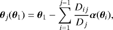
In this section we briefly revisit generalised multi-plane gravitational lens theory (e.g. Blandford & Narayan 1986; Schneider et al. 1992), which considers the fact that a light ray can be bent multiple times by several deflectors during its path. This theory takesinto account the effect of secondary lenses at different redshifts using the thin-lens approximation for every deflector on its redshift plane. The lens equation in this formalism is (following Gavazzi et al. 2008)
 (1)
(1)
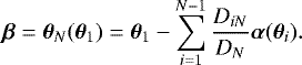
where θ1 is the image position on the first plane (observed image plane), θj is the image position on the jth plane and α(θi) is the deflection angle on the ith plane. In this recursive equation the deflection angle on one plane depends on the deflection angle of all the previous planes. The source position β, which is on the Nth plane, corresponds to
 (2)
(2)
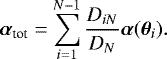
Therefore the total scaled deflection angle αtot is the sum of all the deflection angles on all planes, namely
 (3)
(3)
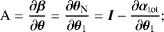
The magnification in the multi-plane case is calculated from the Jacobian matrix obtained by differentiating the total scaled deflection angle αtot, namely
 (4)
(4)
the magnification is
 (5)
(5)
To compute the average surface mass density Σ(<R), we obtain the convergence κ from GLEE and multiply it by the critical surface mass density Σcrit using the definition of convergence,
 (6)
(6)
where Σcrit is
 (7)
(7)
We then computed the average1 surface mass density, namely
 (8)
(8)
In the multi-plane case, these quantities need to be properly defined using the multi-plane formalism: the deflection angle which we obtained the multi-plane κ from is the αtot expressed by Eq. (3). The quantity derived from differentiating this αtot is what we call the “effective” convergence κEff. We then multiplied this quantity by Σcrit to obtain the effective average surface mass density ΣEff(< R). Therefore, this quantity is not a physical surface density, but the gradient of the total scaled deflection angle αtot, which receives contribution from all mass components on all the planes.
2.2 Lens mass distributions
In GLEE, we used parametric mass profiles to portray the cluster members component, the LOS perturber galaxies component, and the contribution of the remaining intra-cluster mass (mainly dark matter) respectively. We modelled the luminous mass component (i.e. members and LOS galaxies) with a truncated dual pseudo-isothermal elliptical mass distribution (dPIE; Elíasdóttir et al. 2007; Suyu & Halkola 2010) with vanishing core radius. Their dimensionless projected surface mass density – convergence – is
 (9)
(9)
where (x, y) are the co-ordinates on the lens plane, θE is the lens Einstein radius, rt is the truncation radius. The mass distribution is then suitably rotated by its orientation angle θ and shifted by the centroid position of the co-ordinate system used. The convergence for a given source redshift zs is
 (10)
(10)
The 2D elliptical mass radius is
 (11)
(11)
and the ellipticity is
 (12)
(12)
where q is the axis ratio. Therefore, the parameters that identify this profile are its central position (xc, yc), its axis ratio q, its orientation θ, its strength θE, and its truncation radius rt.
The 3D density corresponding to this κ is
 (13)
(13)
where r is the 3D radius. As we can see, for r greater than the truncation radius, this density distribution is truncated, that is it scales as r−4. For isothermal profiles there is a direct relation between the value of the velocity dispersion σ of the lens and that of its strength θE (for a sourceat zs = ∞), namely
 (14)
(14)
To model the remaining mass of the cluster, especially the contribution of the dark matter halos, we use a 2D pseudo-isothermal elliptical mass distribution (PIEMD; Kassiola & Kovner 1993) or a softened power-law elliptical mass distributions (SPEMD; Barkana 1998). The convergence of the PIEMD profile, is
 (15)
(15)
where, again, (x, y) are the co-ordinates in the lens plane, Rem is the elliptical mass radius, θE is the lens Einstein radius and rc is the core radius. The mass distribution is then suitably rotated by its orientation angle θ and shifted by the centroid position of the co-ordinate system used. The parameters that identify this profile are its central position (xc, yc), its axis ratio q, its orientation θ, its strenght θE, and its core radius rc. In the case of the SPEMD, there is one additional parameter, which is the slope γ of the profile, since its convergence, is
 (16)
(16)
where q is the axis ratio, rc is the core radius, γ is the powerlaw index, which is 0.5 for an isothermal profile (Barkana 1998).
2.3 Scaling relation
Throughout this work, to reduce the number of model parameters and therefore increase the computational efficiency of our modelling, we assumed scaling relations for the Einstein radii and truncation radii of the cluster members, that is we scaled them with respectto a reference galaxy, which we choose as the cluster member with median luminosity. The scaling was done following Grillo et al. (2015),
 (17)
(17)
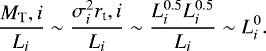
where θE, i and rt, i are the Einstein radius and the truncation radius of the ith galaxy with luminosity Li, and θE,g, rt,g, Lg are the properties of the reference galaxy. This is equivalent to having cluster members with a total mass-to-light ratio  , also known as the tilt of the fundamental plane (Faber et al. 1987; Bender et al. 1992), since
 (18)
(18)
To test how the values of the parameters change if we assume a different scaling relation, we also use
 (19)
(19)
This is equivalent to having cluster members with constant total mass-to-light ratio, since, as shown in Grillo et al. (2015)
 (20)
(20)
2.4 Determination of model parameters
GLEE uses a Bayesian analysis to infer the best-fit parameters, that is those that maximise the likelihood on the image plane (given uniform priors on the parameters), namely the probability of the data (the observed image positions Xobs, which corresponds to θ1 in Sect. 2.1) given a set of parameters η of the model. This likelihood
![Mathematical equation: \begin{equation*}\mathcal{L}(\vec{X}_{\textrm{obs}}|\vec{\eta}) \propto \exp { \left[ -\frac{1}{2}\sum_{j=1}^{\textrm{N_{\textrm{sys}}}} \sum_{i=1}^{\textrm{N_{\textrm{im}, j} }} \frac{| \vec{X}_{i,j}^{\textrm{obs}}- \vec{X}_{i,j}^{\textrm{pred}}(\vec{\eta}) |^2}{\sigma_{i,j}^2} \right] } \end{equation*}](/articles/aa/full_html/2018/06/aa31433-17/aa31433-17-eq22.png) (21)
(21)
describes the offset between the observed  and predicted
  image positions forall the images Nim,j of the observed image system j of Nsys, where σi,j is the observational uncertainty of the ith image of thejth source. We used a simulated annealing technique to find the global minimum and recover the best-fit parameter values, Markov chain Monte Carlo (MCMC methods based on Dunkley et al. 2005) and EMCEE (Foreman-Mackey et al. 2013) to sample their posterior probability distributions. The posterior probability is obtained using Bayes’ Theorem
 (22)
(22)
where P(η) is the prior probability on the model parameters, that we always assume to be uniform. For the centroid position of each halo we use a broad uniform prior range, that is ~ 60″ from the respective BCG centre, and for the axis ratio a range from 0.2 to 1. For the Einstein and truncation radii of all the galaxies and halos we set a minimum prior value to zero, for the orientation of the halos we assumed no boundaries on the priors. The model parameter values we show throughout this work, unless stated otherwise, are the median of the one-dimensional marginalised posterior PDF, with the quoted uncertainties showing the 16th and 84th percentiles (i.e. the bounds of a 68% credible interval). To obtain realistic uncertainties for the model parameters, we ran a second MCMC analysis where we increased the image position uncertainty to roughly the value of the rms, to account for the model imperfections (e.g. lack of treatment for elliptical cluster members, simplistic halo models, neglecting small dark-matter clumps). These new uncertainties are those shown in the tables and used to quantify the ability of the models to recover the input values. The root mean square values are quoted for the best-fit models, and do not depend on the adopted error on the observed image positions. We computed the root mean square error via
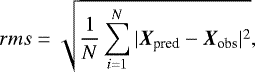 (23)
(23)
with the model-predicted image positions Xpred and the observed image positions Xobs. When the number of predicted and observed image positions of a given image system is not the same, for each observed image in that system GLEE selects the closest predicted image to compute the χ2 of the model. We also used the closest predicted image to compute the rms.
3 Toy models
We begin with simple toy models of lenses at multiple redshifts in order to gain intuition for multi-plane lens modelling. We generated mock lensing observables and analysed the impact of the introduction of multi-plane lenses by fitting the same image positions with both a multi-plane-lens and a single plane-lens model.
3.1 Two lenses at different redshifts
We started our analysis with a simple toy model composed of two lenses (modelled as SISs and denoted respectively as SIS1 and SIS2), at redshifts zSIS1 = 0.5, zSIS 2 = 0.7 aligned along the LOS and with Einstein radii of 2.′′6 and 1.′′6 respectively, and a point source at redshift zs = 2, as shown in Fig. 1. We studied different configurations, in terms of lens location and lensed image positions, and tested how well, for the same simulated observed image positions, we were able to reconstruct the properties of the system using a single lens at zsd = 0.5 whose centre is coincident with the input position of SIS1.
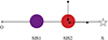 |
Fig. 1 Positional setup of the two lenses. The first lens (purple) is at zSIS1 = 0.5, the second lens (red) at zSIS2 = 0.7. Both the lens are SISs. The dotted arrows indicate the direction in which we shift the second lens to experiment the effects on the image positions and magnification. |
3.1.1 Variation of mass of SIS2
We find that the variation of the mass of SIS2 still allows us to fit the image and source positions and reconstruct the magnification with a single lens, if the two lenses are aligned. Expectedly, we obtain an Einstein radius of the single deflector θE,sd which increases as we increase the mass of the second lens SIS2. The image positions, the magnifications and the source position predicted by the single-lens models can reproduce the input values to the 4th-digit precision.
3.1.2 Variation of position from optical axis of SIS2
Variations in the position of SIS2 with respect to the optical axis (we choose a range of 0.′′ 2–1.′′5) still allow a perfect fit to the same image positions with a single lens (with a 4th-digit precision). The Einstein radius of the single lens θE,sd is unchanged with respect to changes of SIS2’s distance from the optical axis (we kept the Einstein radius of the SIS2 fixed, while its distance to the optical axis is increased). This is probably a result of the particular properties of the SIS profile, where the deflection angle is independent of the location. Moreover, we chose a range where the maximum shift of position of SIS2 is lower than the Einstein radius of SIS1 (θE,SIS1 = 2.′′6). However, we find that the magnification of the multi-plane system decreases as SIS2 moves further away from the optical axis (drops from ten to six for the image with positive parity and from eight to 0.3 for the image with negative parity), while the magnification of the single-plane system stays constant, since θE,sd is itself unchanged.
3.1.3 Variation of redshift of SIS2
Finally, if we shift SIS2 on the optical axis to higher redshifts, we observe that θE,sd decreases, while the magnification increases accordingly for both the multi-plane and single plane lens system, as shown in Fig. 2. Moreover, the predicted source position moves closer to the optical axis when the SIS2 moves to higher redshifts and when the Einstein radius of the single lens decreases.
3.2 Mock cluster lensing mass distribution 2
3.2.1 Input
We now create a more realistic mock system, composed by a cluster at zc = 0.4 with a halo and ten elliptical galaxies having different, realistic luminosities, axis ratios and orientations. We assume a total mass-to-light ratio corresponding to the tilt of the fundamental plane, and we scaled the mass and the truncation radii according to Eq. (17). We added two foreground perturbers at zfd = 0.2, one close and one far away in projection from the cluster centre, and one close-in-projection background perturber at zbd= 0.6. All the perturbers are massive (Einstein radii of 2″) and have the same Einstein radii, random ellipticity (between 0.6 and 1) and orientation, as shown in Table 1. We adopted a SPEMD profile for the halo, and dPIEs for the cluster members and LOS galaxies. We used this configuration to simulate mock lensing data, and we obtained a set of 16 multiple image positions of the three background sources, shown in Fig. 3. We then modelled the parameters, that is all the halo parameters mentioned in Sect. 2.2, the cluster members’ Einstein and truncation radii (with the scaling relation in Eq. (17) unless otherwise stated) and perturbers’ Einstein radius (truncation radius was fixed to 15″), with both the multi-plane set-up and the single-plane set-up (i.e. the cluster only).
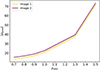 |
Fig. 2 Absolute value of the magnification for the two images of a source at redshift zs = 2 as a function of redshift of SIS2. The lens SIS1 is kept fixed at redshift zSIS1 = 0.5 and SIS2 is free to move along the optical axis within redshift zSIS2 = 0.8 and zSIS2 = 1.5. The predicted magnification shown here corresponds to the multi-plane model, but we observe the same trend for the model with a single lens. |
3.2.2 Full multi-lens-plane modelling
In the full multi-lens-plane model, since it has the same properties as the input (i.e. perturbers, scaling relation for cluster members etc.), we recover, within the errors, the initial parameters we have used to simulate, as shown in the MP-full column of Table 1. The modelled image positions and the magnifications are perfectly fitted, meaning that they have a null total-rms offset.
3.2.3 Single cluster-plane modelling
The single plane case, as shown in column SP in Table 1, shows a shift of the halo centroid position of ~ 1.′′4, due to the removal of the foreground perturber which was lensing it, an overestimation of the halo Einstein radius of ~ 3″. The halo’s profile slope is less peaky in the centre, and it has a core radius that is ~ 2.′′5 bigger. In terms of image positions and magnification, we find that the image positions’ total rms offset is ~ 0.′′55, and the magnification is generally greater, up to three times higher.
3.2.4 Mock cluster model 2: Assuming constant total mass-to-light ratio
In this experiment, we tested how the parameters change if we modelled assuming a different total mass-to-light relation. Wechose a constant total mass-to-light ratio, which scales the Einstein and truncation radii of the cluster members as shown in Eq. (19). If we model the observables with the multi-plane system, we find, as shown in column MP-constML in Table 1, that the halo centroid position is shifted by ~ 0.2″. Even if the lensing effects of the foreground galaxy are still present, the halo is slightly more elliptical and the slope is slightly bigger. The cluster members have instead a bigger Einstein radius and a smaller truncation radius. All the remaining parameters are recovered within the errors. Modelling with the single-plane (SP-constML in Table 1) instead changes the halo centre by ~ 1.′′5, the halo Einstein radius by ~2.′′5, which is less than what we recover in the single-plane with the previous mass-to-light ratio assumption, and underestimates the cluster galaxies masses. This model also predicts a shallower halo profile.
In terms of image positions, we find that the total rms for the multi-plane system is ~ 0.′′12 and the magnification is generally smaller, within a ratio of ~ 0.6–0.8, showing that this approximation works slightly worse than the original total mass-to-light ratio used to simulate. The single-plane system, instead, has a total rms of ~0.′′5, which appears to be less than what we recover using as total mass-to-light the tilt of the fundamental plane. This shows that, in the single-plane case, this approximation works slightly better than the standard SP. This is also confirmed by the magnification, which is still higher, but only up to twice as high. This unexpected behaviour might be explained by the fact that, as shown in Fig. 4, assuming a constant total mass-to-light ratio implies, given the same Einstein radius of the reference member, bigger Einstein radii for the other members (radius of circles in Fig. 4 proportional to Einstein radius). This is compensated by a decrease of the halo Einstein radius, that is, closer to its input value, to preserve the total mass within the total Einstein radius of the cluster. Probably a closer Einstein radius value for the halo is more efficient in reproducing the overall effect on image positions and magnification.
3.2.5 Mock cluster model 2: Assuming spherical galaxies
The next test is to model all the galaxies (members and LOS galaxies) as if they were spherical. The multi-plane system modelling, as shown in the column MP-s in Table 1, shows an offset of the halo centroid position of ~ 0.′′7, and an underestimation of its Einstein radius of ~ 3″. The cluster galaxies and the background perturber have a bigger Einstein radii, while the foreground close-in-projection perturber has a smaller Einstein radii than the original parameter used to simulate. The image position rms is close to the observational uncertainties of ~ 0.′′065, and the magnification is generally smaller, within a factor of 0.7–1. This shows that, despite the low rms, assuming spherical galaxies creates quite a substantial offset in centroid position and Einstein radius. This suggests we should be cautious in interpreting the reconstructed cluster mass distribution, since having small rms, even comparable to positional uncertainty, does not guarantee unbiased recovery of the lens parameters. However, since our model is very simplistic (i.e. few cluster members and very massive perturbers along the LOS), we suspect these results might not be so prominent in more realistic cases where there are many more galaxies and the ellipticity averages out. In the single-plane case, we have that the parameters are consistent, within the errors, to the case with elliptical galaxies and the total rms is ~0.′′55.
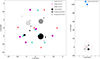 |
Fig. 3 Mock cluster lensing mass distribution 2. The black circles represent the lenses (cluster members), the grey circles the foreground galaxy (darker grey) and the background galaxy (lighter grey). The cyan triangles, magenta squares and red stars represent the images of the three sources, respectively at zs1 = 1.5, zs2 = 2.0, zs3 = 2.5. The circles radii are proportional to the galaxy’s luminosity relative to the BCG (biggest circle). One far-in-projection foreground galaxy, shown in blue in the right panel, was added to this system (100″ away from the BCG). |
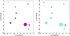 |
Fig. 4 Cluster galaxies’ positional distribution of mock mass distribution 2, in the case of the total mass-to-light ratio equalling the tilt of the fundamental plane (left) and equalling to a constant (right) for the multi-plane case. The circles radii are proportional to the galaxy’s Einstein radius relative to the BCG (biggest circle) mass. |
3.2.6 Mock cluster model 2: Assuming spherical cluster members
To further investigate the spherical assumption on galaxies, we produced a multi-plane model similar to that done previously, but assuming only the cluster members to be spherical. Therefore, the perturbers maintain the original ellipticity that was used in the simulation. As shown in column MP-sm in Table 1, this test still produces an offset in the centroid position, but by only ~ 0.′′4; it underestimates the halo Einstein radius, but by ~1.′′2, and overestimates the cluster member Einstein radius by ~0.′′4, which is, instead, greater than the case where all the galaxies were spherical. This model also still overestimates the background perturber and the far-in-projection foreground perturber mass, but by a smaller amount, and does recoverthe close-in-projection foreground mass. Unlike the previous models, the halo slope in this model is underestimated, which makes the profile smoother. The image position rms is close to the observational uncertainties of ~ 0.′′083, and the magnification is generally smaller, within a factor of 0.7–0.9. As already mentioned in Sect. 3.2.5, we suspect these results will be mitigated in more realistic clusters cases.
3.2.7 Mock cluster model 2: Average surface mass density
To explore the differences in mass among the models, we computed the average surface mass density Σ(< R) (Eq. (8)), as explained in Sect. 2.1. Figure 5 shows the relative error on the Σ(< R), from top to bottom, for both the single plane and multi-plane cluster models as compared to the input. We note that in the bottom panel of Fig. 5, we plot the effective average surface mass density ΣEff(< R), since it contains contributions from both the cluster and the perturbers, which are at different redshifts. We used the cluster redshift and the median source at redshift z = 2 for computing Dd, Ds and Dds for the multi-plane ΣEff(< R). The central panel of Fig. 5 shows, instead, the Σ(< R) of the cluster for the multi-plane model, which we obtained from the convergence κ of the multi-plane best-fit models excluding the LOS perturbers’ contribution. We see that the different models in the top and bottom panels of Fig. 5 tend to agree very well at ~ 10″, which is around the Einstein radius of the system. In the central panel of Fig. 5, however, the model with the spherical galaxies assumption differs by ~10% from the one with elliptical galaxies. This might be due to the fact that, for that multi-plane model, we computed κ for the cluster only, whereas lensing constrains tightly the total κ, including the contribution of the LOS perturbers. This is also confirmed by Fig. 6, where we see that the spherical assumption is always offset from the input model (which has elliptical galaxies and mass-to-light ratio equal to the tilt of fundamental plane). Moreover, it appears that the spherical model MP-s gives more mass to the perturbers, as shown already in Table 1. If we look at the case with spherical cluster members only (MP-sm), we see that the offset to the model is smaller than that of MP-s, where also the perturbers are assumed spherical. From Fig. 7 we see that this is valid also in the single-plane case. Probably leaving to the perturbers their original ellipticity gives them less mass (see Table 1), thus the total cluster mass is recovered better. Finally, we observe that the multi-plane models are generally more peaked in the centre, as compared to single-plane ones, since their core radius is smaller than that of the single plane case (see Table 1).
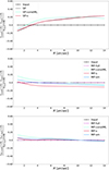 |
Fig. 5 Relative error on the average surface mass density Σ(< R) as a function of radius from the BCG for the best-fit models of Mock mass distribution 2. From top to bottom: single plane cluster, cluster (without LOS perturbers) from multi-plane models, and total multi-plane configuration. In each plot, the lines represent the input (solid black), the multi-plane model (dashed magenta), the single-plane model (dashed black) the model where we assumed constant mass-to-light ratio (light blue), the model where we assumed spherical galaxies (red) and, only in the multi-plane cases, the model where we assumed only spherical cluster members (blue). We note that in the total multi-plane configuration the ΣEff is derived from the total deflection angle and computed for a source at zs = 2, as explained in Sect. 2.1. We observe that at θE,tot ~ 10″ all models converge to a certain value of Σ(< R) and ΣEff in the top and bottom panels, showing that strong lensing provides accurate mass enclosed within the Einstein radius. |
3.2.8 Mock cluster model 2: Generic effects of LOS perturbers in the toy model
We find that the halo orientation and ellipticity are robust parameters. As we also notice in mock cluster mass distribution 1 (discussed in Appendix), they mainly stay, within the errors, close to the original values used to simulate. We also see that constraining the truncation radius of the galaxies rt,g, especially that of the perturbers, is difficult, and we note that multi-plane models are generally better at constraining it than the single plane models (see Table 1). We think this might be caused by the limited amount of multiple image systems andby the fact that the truncation radius is of similar size as the total Einstein radius of the system (~ 15″). However, in general this parameter does not appear correlated to the other parameters, and it is sampled as a flat probability distribution.We also note that the mass of the far away perturber is a quantity that is not generally correlated to the other parameters, except for a slight correlation to the cluster galaxies mass and the halo mass and slope. Moreover, its posterior probability distribution is flat, therefore this quantity is mostly unconstrained. This might be due to the fact that this distant galaxy is very far away from the multiple image region, which in our mock system extends to ~ 15″. In the multi-plane models we find a strong correlation between the core radius and the slope of the halo, which might be due to the fact that if we increase the core radius, the slope of the halo becomes less peaky, and that the background mass is strongly correlated with the mass of the foreground and with the halo mass. In all the single-plane cases, we find slight degeneracies between the halo ellipticity, mass and the cluster galaxies’ mass. These degeneracies, as mentioned in Sect. sectionlinking A.3, would keep approximately the same total mass enclosed within the multiple images. Moreover, in mock cluster massdistribution 1 (discussed in the Appendix) we explore the effect of the single perturber, that is, only foreground and only background. We find that including the foreground is more important for a precise image reconstruction and for recovering the input parameter of the cluster, due to the lensing effect of foreground galaxies on the cluster itself.
4 MACS J0416.1–2403 mass distribution
4.1 Observation of MACS J0416.1–2403
In this section we present our models of the mass distribution of the HFF cluster MACS J0416.1–2403 (from here on, MACS0416), which is a massive luminous cluster at zc = 0.396, with a very large spectroscopic data set along the LOS (Balestra et al. 2016). This cluster, shown in Fig. 8, was first discovered within the MAssive Cluster Survey (MACS) in the X-rays by Mann & Ebeling (2012). It shows an elongation in the NE-SW direction and was firstly identified as a merger. Since its discovery, MACS0416 has been extensively studied (e.g. Zitrin et al. 2013; Jauzac et al. 2014, 2015; Grillo et al. 2015; Diego et al. 2015; Caminha et al. 2017; Hoag et al. 2016; Kawamata et al. 2016; Natarajan et al. 2017; Bonamigo et al. 2017) as it represents an efficient lens for magnifying sources and producing multiple images (strong lensing regime), as shown in Fig. 9. In most recent studies (Grillo et al. 2015; Caminha et al. 2017) the image position was reconstructed with extremely high precision (Δrms ~ 0.′′3 in Grillo et al. (2015), with a set of 30 spectroscopically identified images, and Δrms ~ 0.′′59 in Caminha et al. (2017), with a set of 107 spectroscopically confirmed images), reaching the limit of what can be achieved by neglecting LOS contribution in the modelling. To study the effect of the LOS galaxies, we have created a mock mass distribution by building a model of MACS0416 that reproduces the observables as close as possible, and we use the model parameters to produce simulated observables. We then modelled the mock MACS0416 with different assumptionsand compared them to the input mock model to assess the impact of LOS perturbers, as in previous sections.
Constraints on lens parameters for different models of mock cluster lensing mass distribution 2.
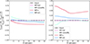 |
Fig. 6 Relative error on the average surface mass density Σ(< R) as a function of radius from the BCG for the multi-plane best-fit models of Mock mass distribution 2. Left: cluster halo only. Right: cluster members only. In each plot, the four lines represent the full multi-plane model (dashed magenta), the model where we assumed constant mass-to-light ratio (light blue), the model where we assumed spherical galaxies (red), and the model where we assumed only spherical cluster members (blue) as compared to the input simulated cluster (solid black). |
4.2 MACS J0416.1–2403 best-fit model
We modelled the mass distribution of MACS0416 with a single-plane setup very similar to that presented by Caminha et al. (2017), but optimised independently with GLEE. This model consists of 193 cluster members, three dark matter halos and it is modelled on a set of 107 images (shown in Fig. 9) corresponding to 37 sources, all of them spectroscopically confirmed. We then included 11 chosen foreground and background galaxies into the model. These are listed in Table 2 and discussed in Sect. 4.2.1. We used truncated dual pseudo-isothermal elliptical mass distributions (dPIEs) to represent the galaxies (members and perturbers), and pseudo-isothermal elliptical mass distribution (PIEMDs) for the halos, as these profiles were shown to reproduce better the observables (Grillo et al. 2015). We assumed all the galaxies to be spherical. The main reason for this choice is that measuring shapes of galaxies in a crowded cluster field is non-trivial and is thus beyond the scope of this work. The halos of galaxies located in the cores of clusters might have been significantly stripped and thus the shapes of these halos might deviate significantly from the shapes of the stellar component (e.g. Suyu et al. 2012; Harvey et al. 2016, among others). Furthermore, we suspect the effects of the ellipticities of the cluster members would average out with the substantial number of cluster members in MACS J0416.1–2403, as opposed to the case in mock mass distribution 2 (Sect. 3.2) where there are few cluster members. Two halos are located on the north-east (halo 1), south-west (halo 2) and centred, respectively, on the northern and southern BCGs. A third smaller halo is located in the eastern part of the northern halo.
To obtain the best-fit model that includes the perturbers, we model the halo parameters (centroid position (xh, yh), axis ratio  , orientation θ, Einstein radius θE,h, core radius rc,h), the Einstein radii and truncation radii of the cluster members and perturbers. We scaled the Einstein radii and truncation radii of the cluster members using the tilt of fundamental plane for the total mass-to-light ratio (Eq. (18)), as described in Sect. 3.2.1, using Eq. (17). This mass-to-light ratio was shown to better reproduce the image position of this cluster by Grillo et al. (2015). As a reference galaxy we used a relatively isolated member (magnitude of 18.1 in the F160W band) which is marked in white in Fig. 8, together with the two BCGs, G1 and G2. We did not include in the scaling relation of the cluster members a luminous galaxy which is very close to the bright foreground galaxy (and also to a less massive foreground galaxy) in the south-west region of the cluster (see Fig. 10). The reason for this choice is that the light contamination from the foreground galaxy in that region does not allow an accurate estimation of the cluster member’s magnitude, which is also affected by the magnification due to the foreground galaxies. We quantified the same magnification effect due to the foreground galaxies on other close-by cluster members, but found that it was negligible. We also find that allowing that particular member to vary freely (both its Einstein radius, and truncation radius) decreases substantially the χ2 of around ~18%. We scaled the Einstein radius and truncation radius of the perturbers as explained in Sect. 4.2.1. We used an error on the images which corresponds to the observational uncertainty ~ 0.′′06 (one pixel). However, we used a special treatment for images with high magnification forming arcs, since they have a more elliptical shape. We therefore introduced elliptical errors for those systems, with the minor axis of around one pixel, the major axis between 0.′′ 2–0.′′4 (depending on the spatial extent of the arc) and orientated along the direction of the arc.
 |
Fig. 7 Relative error on the average surface mass density Σ(< R) as a function of radius from the BCG for the single plane best-fit models of mock mass distribution 2. Left: cluster halo only. Right:cluster members only. In each plot, the three lines represent the single plane model (dashed black), the model where we assumed constant mass-to-light ratio (light blue), and the model where we assumed spherical galaxies (red) as compared to the input simulated cluster (solid black). |
4.2.1 LOS secondary lenses
The secondary lenses are chosen among the brightest (mag < 21.5) and closest to the multiple image region objects of the HST image, selected using near-IR (F160W) luminosities. We expect these brightest LOS galaxies to have the most significant effects on the modelling, compared to other fainter LOS galaxies. For the background perturber we have taken into account the magnification effect due to the cluster lensing. We kept the number of perturbers relatively low (11) for computational efficiency. Figure 8 shows the cluster MACS0416 with the perturbers, indicated by colour depending on whether they are foreground or background galaxies. The brightest foreground perturber in the southern region of the cluster was already included in previous models (Johnson et al. 2014; Richard et al. 2014; Grillo et al. 2015; Caminha et al. 2017), but at the cluster redshift. We included this foreground bright galaxy at its actual redshift z = 0.1124 (first object in Table 2). Each of the 11 LOS perturber has two additional parameters (Einstein and truncation radii), and we scale the Einstein and truncation radii of these LOS galaxies with respect to the brighter ones. We scaled separately the foreground and background, using the definition of apparent magnitude and correcting the observed magnitude of the background for the magnification effect due to the presence of the foreground and the cluster, as follows:
 (24)
(24)
where the flux F
 (25)
(25)
with Dl the luminosity distance to the object. Substituting in the definition of magnitude,
 (26)
(26)
we obtain
 (27)
(27)
If we now want to obtain the luminosity, we revert the equation to
 (28)
(28)
and we scale it with the magnification μ,
 (29)
(29)
where the magnification value for each perturber galaxy is obtained from the multi-plane best-fit model with only the foreground galaxies andthe cluster. Therefore, the scaling is obtained by multiplying the reference quantity to the luminosity ratio Lr as shown in Eq. (17). We let the bright foreground galaxy at z = 0.1124 free to vary, and we scale the remaining two foreground galaxies with respect to the galaxy at zf, ref = 0.1126, and the eight background galaxies with respect to that at zb, ref = 0.5004. The reference perturbers were chosen since they have the greater apparent magnitude among, respectively, the foreground and background LOS galaxies, as shown in Table 2.
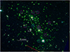 |
Fig. 8 Colour image of MACS J0416.1–2403 obtained through a combination of the HST/ACS and WFC3 filters. We indicate theselected 11 secondary lenses that we included in our model to account for the LOS contribution, using different colours for foreground (cyan) and background (magenta). In green we circle the cluster members. The two BCGs and the reference galaxy we use for the scaling relations are shown in white. North is up and east is left. |
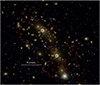 |
Fig. 9 Colour image of MACS J0416.1–2403 obtained through a combination of the HST/ACS and WFC3 filters. We show the selected 107 images we included in our model, corresponding to 37 sources that range from redshifts ~ 1 to ~ 6. The two BCGs are shown in white. North is up and east is left. |
4.2.2 Results of best-fit model of MACS J0416.1–2403
Our best-fit model can reproduce the image positions with an rms~ 0.′′53 (see Fig. 11), that is approximately 8–9 pixels. Previous works with the same set of images (Caminha et al. 2017) was able to reproduce the observed image positions with a rms of ~ 0.′′59; therefore our model with the addition of the LOS galaxies shows an improvement of ~ 0.′′06. Our model has a χ2 ~ 7.5 × 10³. The best-fitmass distribution parameters are shown in Table 3. We remark that 1″ at the redshift of the first foreground galaxy zfd ~ 0.1 corresponds to ~1.8 kpc, while at the cluster redshift zc = 0.396, 1″ corresponds to ~ 5.34 kpc. Therefore, the truncation radius of the brightforeground galaxy is ~300 kpc, which is a typical value for massive galaxies. However, we find from the posterior probabilities that the truncation radii of the LOS galaxies are mostly unconstrained due to the fact that they are isolated galaxies. The truncation radii of the cluster members are instead smaller, due to the tidal stripping of their dark matter halos. Figure 11 shows the observed image positions of MACS J0416.1–2403 and the predicted image positions of our best-fit model, which are in very good agreement, as can also be seen by the histogram of their positional offset. However, our model predicts 106 images of 107 observed, since two images in the north-east region of the cluster are predicted as a unique one (see Fig. 11)2. The predicted magnification of the 106 images is shown in Figs. 12 and 13. One image has a very high predicted magnification ( ), that is not shown in the plot for visualisation convenience3. In Fig. 14, we plot the average surface mass density for the best-fit model of MACS J0416.1–2403. We find that neglecting the LOS contribution does not affect the total Σ reconstruction significantly (see Fig. 14). We also find that most of the contribution on the outskirts (from ~ 20″ from the northern BCG), is due to the halo mass, while in the very centre (~ 5″ from the northern BCG), the contribution of the galaxies is more prominent. We have used the unlensed positions (i.e. those they would have if the perturbers were not there) for the halos and members when computing the average surface mass density of the cluster, halos and members separately. We also computed the velocity dispersion of the cluster galaxies, that, for isothermal profiles, is related to the Einstein radius of the galaxy by
 (30)
(30)
for a source at infinite redshift. The velocity dispersion of a galaxy is also related to its circular velocity by
 (31)
(31)
We then looked (Fig. 15) at the number of galaxies with a certain circular velocity, therefore mass, and we confirm the trend already pointed out by Grillo et al. (2015), that the amount of small mass halos seems to be in better agreement with simulations, whereas we find more high mass sub-halos than predicted by cosmological simulations (details on cosmological simulations can be found in Bonafede et al. 2011; Contini et al. 2012; Grillo et al. 2015). Regarding the radial distribution of substructures, we computed the position of the cluster members by removing the lensing effect of the foreground galaxies, and we compute the radial distance from the barycentre Rb = (1.′′21, −6.′′85), which was obtained by the weighted average
 (32)
(32)
We find our model to slightly underpredict the number of substructures at small radii and at large radii (~ 300–400 kpc), while to overpredict at radii ~ 200–300 kpc with respect to the model of Grillo et al. (2015). This implies a better agreement with cosmological simulations at smaller radii and at large radii, and a worse agreement for radii ~ 200–300 kpc.
Selected secondary lenses added to the MACS J0416.1–2403 cluster, reported in redshift order, from the lowest to the highest.
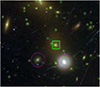 |
Fig. 10 Colour image of MACS J0416.1–2403 obtained through a combination of the HST/ACS and WFC3 filters. Green circles markthe cluster members. The massive member (green square) is not scaled using scaling relations, since it is very close tothe two foreground galaxies (shown in magenta) and its observed magnitude might be affected by their light contamination. |
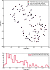 |
Fig. 11 Upper panel: predicted image positions (squares) of MACS J0416.1–2403 MACS J0416.1–2403 and the simulated image positions (triangles) of our MACS model (with introduced gaussian scatter), in comparison to the observed image positions (circles) of MACS J0416.1–2403. Lower panel: positional offsets between the observed and the model-predicted image positions. The rms for our best-fit model of MACS J0416.1–2403 is ~ 0.′′ 53. |
4.3 Mock MACS input
Our best-fit model of MACS0416 and its environment can reproduce the image positions with a rms~ 0.′′53 (see Fig. 11), which is, as already mentioned, the current best-fit model obtained with this set of images. Our set of simulatedconstraints are the 106 predicted image positions from the best-fit model of MACS J0416.1–2403. Since one image of one system was not predicted by our model (see Sect. 4.2.2 for discussion), we decided to tweak the observed position of the third image manually in a way that its position was on the other side of the critical curve with respect to the second image and therefore such that it was predicted by our best-fit model. We then used the image position predicted by best-fit MACS J0416.1–2403 model as the 107th constraint for creating the mock system that we call mock MACS, making our set of constraints to a total of 107 images. As mentioned before, the images’ positional uncertainties corresponds to the observational uncertainty ~ 0.′′06, but we used a special treatment for images with high magnification forming arcs, introducing elliptical errors for those systems, as explained in Sect. 4.2. To obtain the simulated image positions, we then shifted the 107 predicted image positions (of the best-fit model) by a random number, drawn from a 2D-Gaussian distribution with σ =0.′′06, in both x and y direction to introduce a random scatter. In the case of highly magnified images forming arcs, we draw random numbers from a 2D elliptical Gaussian distribution, with σ1, σ2 equal to the minor and major axis of the error ellipses on those images. We then rotated the Gaussian to align with the direction of the arcs, since arcs are tangentially orientated. We used these 107 shifted image positions as our observables. The initial χ2 of the input mock MACS cluster is 246.
Constraints on lens parameters for our model of MACS J0416.1–2403 mass distribution (including three dark matter halos, 193 cluster members, three foreground galaxies and eight background galaxies).
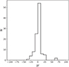 |
Fig. 12 Predicted magnification for the best-fit model of MACS J0416.1–2403. There is one image with predicted magnification of ~4 × 10⁴ (not included in our plot for visualisation convenience), which is one of the arc-shaped images in the north-east region (− 20″, 20″) of MACS J0416.1–2403, as shown in Fig. 11. |
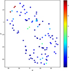 |
Fig. 13 Magnification for the image positions predicted by best-fit model of MACS J0416.1–2403. There is one image with predicted magnification of ~4 × 10⁴ and one withpredicted magnification of ~600 whose magnification value was set to the border value of μ = 65 for visualisation convenience. The two images are in the systems with high magnification and whose positional uncertainty was treated as elliptical due to their arc-like shape. |
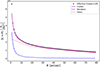 |
Fig. 14 Average surface mass density Σ(< R) as a function of radius (from G1) for the best-fit model of MACS J0416.1–2403 for the total mass of the cluster (magenta line), for the cluster members (dashed blue) and for the dark matter halos (dotted red). The black points represents the effective average surface mass density Σeff (< R) (for source at redshift zs = 3) of the cluster and the LOS galaxies, as explained in Sect. 2.1. Of particular interest is the Σ(< R) within ~80″, which approximately corresponds to the HST FoV at z = 0.396 (~420 kpc). |
4.4 Mock MACS models
Once we had simulated a set of images (107 in total, from 37 sources), we modelled all the halo parameters (centroid position, ellipticity, orientation, Einstein radius, core radius) and the Einstein radii and truncation radii of the cluster members and of the perturbers (see Table 4), with different assumptions to assess the effect of these LOS perturbers. We modelled the mock MACS mass distribution using:
- 1.
MP-full: the full multi-plane treatment, i.e. including all the LOS perturbers at the different redshifts;
- 2.
SP1: assuming only the bright foreground pertuber at the cluster redshift (similar to models in Johnson et al. 2014; Richard et al. 2014; Grillo et al. 2015; Caminha et al. 2017);
- 3.
SP: assuming no LOS perturbers, and including only cluster members;
- 4.
MP-fore: multi-plane including only the three foreground galaxies;
- 5.
MP-back: multi-plane including only the eight background galaxies;
- 6.
MP-constML: full multi-plane with different scaling relation, that is, using constant mass-to-light ratio as shown in Eq. (19);
- 7.
SP-constML: single plane using constant mass-to-light ratio (Eq. (19)).
We describe the results of each of the models below.
4.4.1 MACS MP-full model results
In the case of the multi-plane modelling, where we modelled the parameters in the same set-up as the input, we recover, within the 1σ uncertainties, the input parameters, as shown in Table 4. The rms of this model is 0.08″, which is very close to the observational uncertainty. We see that the offset between predicted and observed image positions is very small (Fig. 16) and the distribution of predicted and observed magnification ratio is centred around 1 with very small scatter in the tails, as shown in Fig. 17. One of the images with high magnification (and therefore elliptical errors) is predicted to have a different image parity than observed. This is due to the fact that it is close to a critical curve, and a slight change on the model can change its relative position with respect to the curve.
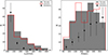 |
Fig. 15 Number of sub-halos as a function of the projected distance from the cluster lens centre (right) and as a function of circular velocity (left) within an aperture of ~ 400 kpc for our best-fit model of MACS J0416.1–2403 (grey filled) as compared to the model of Grillo et al. (2015) (red) and to the median values and the 1σ uncertainties obtained from cosmological simulations used therein (Bonafede et al. 2011; Contini et al. 2012; Grillo et al. 2015). |
4.4.2 MACS SP1 model results
If we model the input mass distribution keeping only the brightest foreground at the cluster redshift (similarly to what wasdone in Grillo et al. 2015; Caminha et al. 2017), we find that the mass of this perturber is decreased. If we look at the scaled Einstein radii of the perturbers, as shown in Eq. (A.1), using zs = 3 (roughly the mean redshift), we see that the difference is less significant, but still the scaled Einstein radius at the real redshift is higher than that atthe cluster redshift. This mass is compensated by an increase in the mass of the southern halo and of the peculiar member (Fig. 10) that has a freely varying mass profile (without scaling relation imposed) due to its proximity to the bright foreground, which is anyway not substantial. However, most of the parameters are recovered. The total rms is ~ 0.2″, as shown in Table 4. This model is however pretty good at predicting the image positions and magnification (magnification ratio median ~ 0.97 as shown in Table 5), and does not show any parity flip in any of the predicted images.
4.4.3 MACS SP model results
In the single plane model, which includes only the cluster, the lack of the LOS galaxies’ mass is compensated by an increase in the mass of the cluster members and halos. This model also shifts the centroid position of the southern halo (becoming closer to the bright massive foreground perturber) and of the smaller halo by almost 1′′. The total rms of this model is ~0.′′32, which is very close to the model precision reached by the single-lens-plane models in recent years. Therefore, residual rms between the observed image positions and the image positions predicted by single-lens-plane models can actually be due to the lack of appropriate treatment of the lens environment (as previously suggested by e.g., Jullo et al. 2010). Moreover, this shows that including the LOS galaxies at the wrong redshift performs better than not including them at all (Table 4 and Sect. 4.4.2). However, the reconstruction of magnification, and therefore the intrinsic brightness of the source, is still possible with the single plane models with an error of ~ 10%. Some more care is needed with images close to critical curves and highly magnified, some of which are predicted to have an opposite image parity in this model as well.
4.4.4 MACS MP-fore model results
If we include only the foreground objects at their correct redshift, we find a slight increase of mass in both the members and the halos, to compensate for the lack of the background perturbers, but we can still recover the input within 1–2σ, as shown in Table 4. The rms of this model is 0.′′ 11, which is also quite close to the observational uncertainty. As in the MP-full model, we find that the offset between predicted and observed image positions is very small and the distribution of predicted and observed magnification ratio is centred around one with very small scatter in the tails, as shown in Fig. 17 and Table 5. Moreover, the same image as in Sect. 4.4.1 is predicted with opposite image parity.
4.4.5 MACS MP-back model results
In the case of the multi-plane modelling with only the background galaxies, we find that the rms is ~ 0.′′3, as in the single plane model. We see that the centroid of the two massive halos are shifted by ~ 1′′, because the model did not take into account the lensing effect of the foreground galaxies. Moreover, to account for the lack of foreground, we find that the members and the southern halo are more massive. We note that this is probably due to the fact that the two most massive foreground galaxies are in the southern region of the cluster. Magnification is reconstructed with ~ 10% error, and this model predicts an image with flipped parity, which is very close to the southern BCG, and thus more sensitive to the increase in mass of members and of the southern halo.
4.4.6 MACS MP-constML model results
If we scale the cluster members and LOS galaxies assuming a different mass-to-light ratio, as for example that of Eq. (19), we find, as expected, that the offset in the predicted and observed image positions is greater than that of the multi-plane model, and it is 0.′′2. As shown inFigs. 16 and 17, the image positions and magnification are, overall, quite well reconstructed. However, in this case we have five images that show a flip in parity, one of which is very close to the southern BCG and is very highly magnified, and the others are part of the system in the north-west region of the cluster, which shows eight images of two clumps of the same source galaxy around two cluster members (system 14 in Caminha et al. 2017, more detailed discussion in Sect. 4.4.9).
Constraints on lens parameters for different models of the mock MACS mass distribution (three dark matter halos, 193 cluster members, three foreground galaxies and eight background galaxies).
4.4.7 MACS SP-constML model results
If we model the input mass distribution with the single plane model and a constant mass-to-light ratio, as in Eq. (19), we find that the image positions are predicted with an overall rms of ~ 0.′′45. This model is, expectedly, the worst at reproducing the image positions and magnification, and even has two predicted pairs of images on the same side of the critical curves. These images belong to the system of multiple images already mentioned in Sect. 4.4.6 (system 14 in Caminha et al. 2017) that correspond to the same source at z = 3.2213. We show the critical curves of that region in Fig. 20 (right panel). and we discuss in Sect. 4.4.8. It also predicts twoof the images with high magnification with a parity flip with respect to the input magnification.
4.4.8 Results
As expected, the multi-plane model is the one that reproduces the image positions best, with a rms of around ~ 0.′′08, value similar to the observational uncertainty. However, accounting for the perturbers’ mass, even if at the wrong redshift (as in model SP1 in Fig. 16), allows the images positions to be reproduced better among the single plane models, with a rms of ~ 0.′′2. The standard single-plane model (SP) has a rms of ~0.′′32. We therefore suspect that part of the offset in single plane models of galaxy clusters might actually be due to the exclusion of the perturbers. We also explored the effect of taking into account only the foreground and background galaxies, and we find that the inclusion of the foreground is more important for a better fit of the observables, confirming what was found for mock mass distribution 1 (discussed in the Appendix) and in McCully et al. (2017), for a more simplistic mock cluster. Actually, for the mock MACS we find that including only the background gives a comparable rms to the single plane models, in other words, not including any LOS galaxy at all. Modelling with the wrong scaling relation, as expected, increases the offsets of the predicted and observed image positions even more, for both the multi-plane and single plane model.
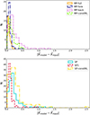 |
Fig. 16 Positional offset of the simulated observed vs predicted image positions of the different models of mock MACS. Top panel: multi-plane models, and bottom panel: single plane models. As expected, the full multi-plane model (black) is the one thatreproduces the image position more closely. |
Magnification ratios between the reconstructed and input magnifications for different mock MACS models.
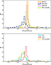 |
Fig. 17 Magnification ratio of the different mock MACS models and the input mock MACS. Top panel: multi-plane models, andbottom panel: single plane models. Interestingly, some images are predicted with high magnification ratio, and some are predicted with a different parity. These images are all the arc-shaped images that lie close to the critical curves. |
4.4.9 Source magnification reconstruction
As for the image positions, the magnification is reconstructed with different precision by the different models. Figure 17 shows the magnification ratio (predicted vs. input) distribution for the different models. We find that the MP-full model distribution is centred around one, showing that this model is the best at reproducing the input magnification. Also the MP-fore and SP1 models are able to reproduce the magnification quite well, with a median ratio of ~ 0.97–1, as shown in Table 5. All the other models tend to predict a lower magnification than the input. In Table 5 we list the median values of the magnification ratio distributions and the respective 1σ uncertainties (16th and 84th percentiles). However, all the distributions have median values within 0.90–1.00, therefore the median error on the magnification reconstruction is still within ~ 10%. Interestingly, some image systems with high magnification and on (or close to) a critical curve, in almost all the models are predicted with a high magnification ratio and/or with a parity flip (we do not show these outliers in Fig. 17 for ease of visualisation). An example of a system with high magnification ratio and parity flip is shown in Fig. 20. In this figure we show the eight simulated observed images of two source clumps of a galaxy at redshift zs = 3.2213, which are located in the north-west region of the cluster (system 14 in Caminha et al. 2017). The multiple images of this source galaxy are located in the neighbourhood of two cluster members (cyan squares in Fig. 20), that act as strong lenses for that particular source. The images are highly magnified and form arcs around those members, and they are very sensitive to the shape of the critical curves due to the presence of those members. If we look at the left panel of Fig. 20 (corresponding to the input model), we see that a pair of images (30c, 31c) are predicted to be on different side of critical curves, with respect to the right panel (corresponding to the SP-constML model). Therefore, in the SP-constML model their predicted image positions coincide with those of, respectively, image 30b and 31b. If we compare the input with the central panel (MP-constML model), we see that in this case the images 30c and 31c are closer to the critical curves, so they are predicted with a much higher magnification. Indeed, as already shown in Sect. 3.2.4, changing the mass-to-light ratio with which we scaled the Einstein and truncation radii of the cluster members, increases or decreases the mass of the members, and consequently changes the shapes of the critical curves for those members, affecting the relative position with respect to critical curves of images nearby. In the model of Caminha et al. (2017), these two cluster members were considered as free parameters instead of being scaled with the other members, since they are the main contributors to the creation of the multiple images of this system (system 14 in Caminha et al. 2017). In general, we suspect images close or on the critical curves need to be treated carefully when trying to reconstruct the intrinsic brightness of the background sources.
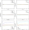 |
Fig. 18 Relative error with respect to the input mock MACS cluster on the average surface mass density Σ(< R) as a function of radius (from G1) for the multi-plane MP (left panels) and single-plane SP (right panels) best-fit models of the mock MACS mass distribution compared to the input model (in dotted black). Upper panels: relative error on the Σeff (< R) (for source at redshift zs = 3) for the total cluster, i.e. halos, members and perturbers. Central panels: relative error on the average surface mass density of the halos for the different models. Bottom panels: relative error on the average surface mass density of the cluster members only. We note that in the total multi-plane configuration the Σeff (< R) is relative to the total deflection angle, as explained in Sect. 2.1. |
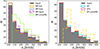 |
Fig. 19 Number of sub-halos as a function circular velocity for our multi-plane (left) and single plane (right) models within an aperture of ~400 kpc. Surprisingly, the model that reproduces better the input is the SP1 model, instead of the MP-full. However, these results are related to the best-fit models and we suspect this might be a coincidence specific to the configuration of MACS J0416.1–2403. |
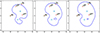 |
Fig. 20 Critical curves for the region of the multiple images of the source galaxy at zs = 3.2213 of our mock MACS models: MP-full (left), the MP-constML (centre) and the SP-constML (right). The different clumps of the source are labelled with different numbers (30 and 31). |
4.4.10 Mass reconstruction
Figure 18 shows the relative error on the average surface mass density for our models as compared to the input mock MACS cluster. We do not observe significant differences among the different models for the total Σ(< R), which reaches a maximum relative error of 0.6 in the cluster core, probably since the number of the perturbers is much smaller than the total cluster mass, therefore they do not contribute significantly to the total mass load. Moreover, all the models agree quite well in the region of the Einstein radius of the cluster, since the mass within the Einstein radius is the quantity that lensing constraints tightly. If we look at the single matter components, that is, only the halos (central panel) and only the members (bottom panel), we find slight differences among the models, especially in the inner part of the cluster, while in the outskirts they all agree quite well. The models that are slightly different from the input are, among the MP models, the MP-back and MP-constML, in both the halos and cluster members Σ(< R). The model MP-back, as we already saw from the positional offset (Table 4 and Fig. 16), is the worst at reproducing the observables among the MP models. This tells us that including only the background perturbers can even perform similarly to the SP model, in which they are not included at all. This implies that the average surface mass density can be similar to that of the SP model (as shown in Fig. 18). Assuming a different mass-to-light relation makes the halos Σ(< R) steeper within the inner part of the cluster, and the cluster members’ one less peaky. We see the same trend in the SP case.
Despite these slight differences, the overabundance of galaxies at the centre of MACS0416 in observations compared to simulations noted in Grillo et al. (2015) is robust against the presence of LOS perturbers. Figure 19 shows the number of cluster members as a function of their circular velocity. If we compare it to the input, we see that most of the multi-plane and single plane models do not change substantially the overall velocity dispersion distribution of the members, showing that this is robust even though the model is not complete. However, we see that both in the single and multi-plane case, if we assume a wrong scaling relation, the distributions tend to prefer more massive galaxies (around 100 km s−1 in the multi-plane case and even 200 km s−1 in the singleplane case). Thus, the choice of scaling relation could potentially alleviate the tension in the disparate numbers of massive galaxies and sub-halos in the inner parts. Encouragingly, our simulations suggest that the χ2 of the model fit could possibly be used to probe the underlying scaling relation. It is worth exploring further scaling relations of the cluster galaxies in future models of MACS J0416.1–2403.
5 Summary
In this work we explored the effects of the LOS galaxies in strong gravitational lensing modelling of galaxy clusters. We simulated different galaxy clusters and their environment, building models of increasing complexity and realism, that we used to simulate strong lensing observables. We then determined the lensing halos’ and galaxies’ parameters with different assumptions and compared to the input simulated cluster to assess the effects of the LOS perturbers.
The simulated system mock cluster mass distribution 2 is composed of a cluster at zc = 0.4 with a halo and ten elliptical galaxies having different, realistic luminosities, axis ratios and orientations. We assumed a total mass-to-light ratio corresponding to the tilt of the fundamental plane. We added two foreground perturbers at zfd = 0.2, one close and one far away in projection, and one close-in-projection background perturber at zbd = 0.6. All the perturbers have equal, large mass, random ellipticity (between 0.6 and 1) and orientation. We used this configuration to simulate mock lensing data, and we obtained a set of 16 multiple image positions of three background sources. In this mock system we explored the effect of different mass-to-light relations and the spherical-elliptical galaxies assumption. We find that:
- 1.
Isolated perturbers that are far-in-projection (ten times or more) from the multiple image region do not affect substantially the other parameters’ values. Indeed their posterior probability is sampled as flat and they do not look correlated to other parameters.
- 2.
In multi-plane modelling, assuming spherical galaxies (both members and perturbers) recovers different profile parameters than the input, and has generically lower magnification. Despite this, the multi-plane reconstruction has a rms very close to the observational uncertainty. Therefore, one needs to be careful in interpreting the reconstructed mass distribution and magnification, as the goodness of fit does not allow to distinguish between spherical and elliptical galaxies. However, the difference in the parameters is less prominent when only the cluster members are treated as spherical. This might be due to the fact that the perturbers of this model are very massive and very close to the cluster centre, therefore they have a large effect on the total mass reconstruction. Moreover, we suspect this effect might depend on the simplicity of our model and might be mitigated in more realistic clusters with higher number of cluster members.
- 3.
Multi-plane models have a peakier average surface mass density than single plane models, which insteadshow a shallower profile. However, all the average surface mass density values match at R ~ 10″, which is the total Einstein radius of the cluster. This shows that the projected total mass enclosed within the Einstein radius - the quantity that strong gravitational lensing constraints tightly - is well reconstructed by all these models.
The other simulated cluster we studied is a realistic model of the HFF cluster MACS J0416.1–2403, labelled mock MACS, which we built using 107 spectroscopically confirmed multiple images from 37 sources (with 1 < zs < 6) as constraints, and then modelling the three halos (two located in the NE, and one in the SW direction), the 193 spectroscopically confirmed cluster members, and the LOS galaxies’ profile parameters. We assumed the cluster members and LOS galaxies to be spherical. We find that our mock of MACS J0416.1–2403 which includes 11 LOS perturber galaxies is able to reproduce the real cluster’s observables with a rms of ~ 0.′′53. We then modelled this simulated mock MACS cluster to assess the impact of LOS galaxies. Our results can be summarised as follows:
- 1.
Neglecting the cluster’s LOS environment leads to a rms of ~0.′′3 in the offset distance between observed and modelled image positions.
- 2.
The inclusion of LOS galaxies in the cluster modelling at the wrong redshift (i.e. at cluster redshift) reproduces the observedimage positions with a rms of ~0.′′20.
- 3.
We find that foreground perturbers have a more significant effect than the background. However, since in this case the discrepancy is more prominent (including only the background is comparable to not including it at all), we ascribe it also to the particular configuration of the cluster.
- 4.
Neglecting the lensing environment or assuming it at the wrong redshift does not affect the reconstruction of the magnification of background sources substantially (errors within ~10%). However, apart from the full multi-plane reconstruction, all the other models tend to underpredict the magnification. We also find that systems with high magnification, or in general close to critical curves, are more sensitive to the different assumptions on the modelling. Indeed, since strong lensing is a highly non-linear effect in these regions, small changes in the parameter values can cause changes on the critical curves positions. These can lead to a much higher predicted magnification and may also cause a flip in image parity.
- 5.
We do not observe a substantial difference in the average surface mass density of the cluster among the various mass models we have considered, probably because these perturbers are very small compared to the total cluster mass. Thus, the overabundance of galaxies at the centre of MACS0416 in observations compared to simulations noted in Grillo et al. (2015) seems robust against the presence of LOS perturbers. However, the mass function of the cluster members depends on the assumed scaling relations. The dependence can be partly mitigated by using the goodness of fit (χ2) of the multiple image positions, since the ‘true’ scaling relations generally lead to lower χ2.
- 6.
We find a correlation between the masses of the foreground LOS perturber galaxies and the halos’ centroid co-ordinates. We also see that the Einstein radius of the different mass components are anti-correlated among each other, since a decrease of mass in one can be compensated by an increase in another component. Moreover, the Einstein radius and truncation radius of the galaxies are correlated with each other.
- 7.
Assuming different scaling relations can lead to very different results for the mass of the members and of the halos, and therefore can change the substructure distribution quite significantly.
Finally, from our best-fit model of MACS J0416.1-2403 we find that, for this particular cluster, the total rms does not decrease substantially after the inclusion of LOS galaxies with respect to single plane models. This suggests that the dynamic and turbulent nature of this cluster is still probably not well depicted by, for example, the simplistic model of the halos. For future model improvements of this cluster those effects would need to be accounted for. We also find that using the correct scaling relations is crucial, especially for reconstructing the sub-halo mass function. Therefore, we conclude that the main contribution to the residual rms for this particular cluster is not due to LOS galaxy, and future models will have to move towards including more complex halo shapes, accounting for the ellipticity of galaxies and improving the scaling relations for the cluster members.
Acknowledgements
GC and SHS thank the Max Planck Society for support through the Max Planck Research Group for SHS. GC acknowledges Prof. Alexandre Refregier and Dr. Adam Amara for the helpful discussions. We thank the anonymous referee for the helpful comments that significantly contributed to improving the quality of the publication. CG acknowledges support by VILLUM FONDEN Young Investigator Programme grant 10123. GBC, AM and PR acknowledge financial support from PRIN-INAF2014 1.05.01.94.02.
Appendix A Mock cluster lensing mass distribution 1
A.1 Input
The simulated mock cluster lensing mass distribution 1 is that of a cluster at redshift zc = 0.4 and two galaxies, a foreground galaxy at zfd = 0.2 and a background galaxy at zbd = 0.6, that are close in projection to the cluster and that we treat as perturbers. The cluster is composed of five galaxies and a dark matter halo. The input parameters are summarised in Table A.1. We assumed all the galaxies in the cluster to have the same luminosity, therefore same mass, for simplicity, and same truncation radius, that we fix to 15″. We put three different point sources (S1, S2, S3) at different redshifts (zs1 = 1.5, zs2 = 2, zs3 = 2.5) and simulate their image positions in the case of the multi-plane configuration. We find that each source is mapped into five images, for a total of 15 images, and used these image positions as our observables. The set-up of this model is illustrated in Fig. A.1.
Constraints on lens parameters for different models of mock cluster lensing mass distribution 1.
A.2 Full multi-lens-plane modelling
We optimised the free parameters of the multi-plane model (Einstein radius of the foreground, background and cluster galaxies, and all the parameters of the halo profile - Einstein radius, position, ellipticity, orientation, core radius and slope) by maximising the likelihood in the image plane. We used simulated annealing to find the global minimum and recover the best-fit parameter values. In this case, since we simulated the image positions with the multi-plane model, we recovered, within the uncertainties estimated by MCMC sampling, the initial parameters we have used to simulate, as shown in Table A.1. The modelled image positions and the magnifications are perfectly fitted, with a null total-rms offset. We find a strong correlation between the mass of the halo and its axis ratio and between the core radius of the halo and the slope of the halo profile. We also find a strong anti-correlation between the centroid position of the halo and the mass of the foreground galaxy, which is explained by the fact that the centroid position is lensed by the foreground galaxy, and between the mass of the cluster galaxies and the axis ratio of the halo. We also find that the mass of the background lens is strongly anti-correlated with the halo mass, core radius and slope, that could also be explained as a lensing effect by the cluster.
A.3 Single-plane modelling
We then removed the foreground and background lens and fit the same image positions with the cluster alone. We varied the cluster parameters and find, as shown in Table A.1, that the halo is still orientated along on the x direction, and the ellipticity is recovered within the errors. However, its centroid position is offset of ~1″ in both x and y direction, its mass is bigger and its core radius is larger by 4″, making the profile less peaky in the centre. Moreover, we recover a smaller mass for the cluster galaxies. In this case we find an additional strong anti-correlation between the halo and the cluster galaxies Einstein radius, which was not so prominent in the multi-plane system. This could be explained as the removal of the two LOS perturbers influences the distribution of the mass between the two remaining mass components, the halo and the cluster galaxies. Moreover, we find degeneracies between the axis ratio and the Einstein radius of the cluster and between the latter and the cluster galaxies’ Einstein radius, since these degeneracies would keep approximately the same total mass enclosed within the multiple images. This, indeed, is what strong lensing constrains tightly. As for the image positions, the single lens systems predicted images are all offset by <0.′′8 in both x and y direction. In terms of total-rms, the image offset is ~0.′′4. The magnification of the single plane configuration appears to be in general different, within a ratio of 0.8 to 1.8 with respect to the input.
 |
Fig. A.1 Mock cluster lensing mass distribution 1. The black circles represent the lenses (cluster members), the grey circles the foreground galaxy (darker grey) and the background galaxy (lighter grey). The cyan triangles, magenta squares and red stars represent the images of the three sources, respectively at zs1 = 1.5, zs2 = 2.0 and zs3= 2.5. |
A.4 Cluster and single perturber modelling
To investigate the effects of the single perturbers we model the same system with the cluster and the foreground lens only and the cluster and the background lens only, respectively. We find that the addition of the foreground perturber to the single-plane model allows us to recover parameters that are more similar to that of the multi-plane model. Indeed, as shown in Table A.1, the halo centroid position is offset by only ~ 0.′′25, its mass is not as big as that of the single-plane model, and the halo slope isrecovered within the error. If we include only the background perturber, instead, we get the same parameter values, within the errors, as that of the single plane model, confirming results from previous studies (e.g McCully et al. 2014), which showed thatforeground perturbers have a more significant effect on themodelling compared to the background ones. In terms of image positions rms, we find a total rms of 0.′′ 18 for the multi-plane model with only the foreground galaxy, while a total rms of ~0.′′4 for the model with only the background galaxy, showing that the additionof the foreground perturber is more significant for a good fit ofthe image positions.
A.5 Effect of individual perturber
Before moving to a more realistic model, we performed a test to further investigate the effect of the individual perturbers along the LOS. We used the mock cluster lensing mass distribution 1 and we increase the mass of the background perturber such that the scaled Einstein radii of the two perturbers, for the intermediate source at zs2 = 2, is equal, namely
 (A.1)
(A.1)
We resimulated the three sets of multiple image positions using Eq. (17). We then repeated the analysis from Sect. A.4 and we find that the perturber in the foreground is still more significant (rms ~ 0.′′32) than the background (rms ~0.′′38), but this effect is less prominent. This is due to two main factors: first that we have equated the strength of the two perturbers, but they are still at different locations with respect to the cluster centre; second is the lensing effect that the foreground has on the cluster. Moreover, in order for the scaled deflection angle of foreground and background galaxy to match, the background mass should be substantially larger than the foreground, meaning with an Einstein radius of ~ 1″ bigger than that of the foreground. So for typical scenarios where foreground galaxies have similar (or higher) masses as background galaxies, we should pay more attention to the foreground lenses.
A.6 Truncation radius
We tried to model the truncation radii of the galaxies, that is, roughly the half-mass radius (Elíasdóttir et al. 2007). At first we allowed the truncation radii of all the cluster galaxies (which we assumed to be equal) and of the two perturber galaxies to vary and we find that they are actually very difficult to constrain. We then fixed the truncation radii for the two perturber and model varying the truncation radius only for the cluster galaxies. In this case we find that the truncation radius posterior has a flat distribution. We therefore suspect that its value does not really affect the parameter modelling, as long as it is not significantly different from its true value. This is probably due to the limited amount of information and to the limited extent of the multiple image region (~15″) of the system, since in this particular mock configuration we chose the truncation radius for cluster members to be comparable to the size of the multiple image region. To explore this further we modelled the multi-plane system keeping all the truncation radii fixed to
10″, instead of the input 15″, value that is outside of the 1σ confidence intervals for the posterior probability distribution of the cluster members’ truncation radius. We find that this wrong choice of truncation radii makes the estimation of the halo mass wrong by ~ 1.′′4 and that ofthe cluster galaxies by ~ 0.′′13, so non-negligible, as shown in Table A.1.
A.7 Conclusions
The simulated system mock cluster mass distribution 1 is composed of a cluster, at zc = 0.4, with five spherical galaxies of equal luminosity and mass, and one dark matter halo with an Einstein radius of 10″. Its environment is constituted by two close-in-projections LOS galaxies, one foreground zfd = 0.2 and one background zbd = 0.6, with equal, large mass. Our observables are a set of 15 images fromthree sources at redshifts, respectively zS1 = 1.5, zS2 = 2.0, zS3 = 2.5. For this cluster we studied the different effects of foreground and background perturbers. We conclude that:
- 1.
Foreground perturbers have a more significant effect in the modelling than the background, for a given equal mass, and their inclusion reproduces the observed image positions more accurately. This might be due to their lensing effects on the observed image positions. Moreover, foreground perturbers have lensing effects on the halos, affecting their centroid position and shape. If we try to equate the scaled Einstein radius (Eq. (A.1)) of foreground and background perturbers we see that this trend is slightly attenuated, but still visible.
- 2.
The truncation radius of the perturbers does not affect substantially the lensing model, since its extent is comparable to that of the multiple image region. Indeed its posterior distribution appears flat and does not appear to be correlated to the parameters of other profiles.
This is also confirmed by the mock MACS model, as discussed is Sect. 4.4.8.
References
- Balestra, I., Mercurio, A., Sartoris, B., et al. 2016, ApJS, 224, 33 [Google Scholar]
- Barkana, R. 1998, ApJ, 502, 531 [NASA ADS] [CrossRef] [Google Scholar]
- Bender, R., Burstein, D., & Faber, S. M. 1992, ApJ, 399, 462 [NASA ADS] [CrossRef] [Google Scholar]
- Blandford, R., & Narayan, R. 1986, ApJ, 310, 568 [NASA ADS] [CrossRef] [Google Scholar]
- Bonafede, A., Dolag, K., Stasyszyn, F., Murante, G., & Borgani, S. 2011, MNRAS, 418, 2234 [NASA ADS] [CrossRef] [Google Scholar]
- Bonamigo, M., Grillo, C., Ettori, S., et al. 2017, ApJ, 842, 132 [NASA ADS] [CrossRef] [Google Scholar]
- Bouwens, R. J., Bradley, L., Zitrin, A., et al. 2014, ApJ, 795, 126 [NASA ADS] [CrossRef] [Google Scholar]
- Caminha, G. B., Grillo, C., Rosati, P., et al. 2016, A&A, 587, A80 [NASA ADS] [CrossRef] [EDP Sciences] [Google Scholar]
- Caminha, G. B., Grillo, C., Rosati, P., et al. 2017, A&A, 600, A90 [NASA ADS] [CrossRef] [EDP Sciences] [Google Scholar]
- Coe, D., Zitrin, A., Carrasco, M., et al. 2013, ApJ, 762, 32 [NASA ADS] [CrossRef] [Google Scholar]
- Contini, E., De Lucia, G., & Borgani, S. 2012, MNRAS, 420, 2978 [NASA ADS] [CrossRef] [Google Scholar]
- D’Aloisio, A., Natarajan, P., & Shapiro, P. R. 2014, MNRAS, 445, 3581 [NASA ADS] [CrossRef] [Google Scholar]
- Diego, J. M., Broadhurst, T., Molnar, S. M., Lam, D., & Lim, J. 2015, MNRAS, 447, 3130 [NASA ADS] [CrossRef] [Google Scholar]
- Dressler, A. 1984, ARA&A, 22, 185 [Google Scholar]
- Dunkley, J., Bucher, M., Ferreira, P. G., Moodley, K., & Skordis, C. 2005, MNRAS, 356, 925 [NASA ADS] [CrossRef] [Google Scholar]
- Elíasdóttir, Á., Limousin, M., Richard, J., et al. 2007, ArXiv e-prints [arXiv: 0710.5636] [Google Scholar]
- Faber, S. M., Dressler, A., Davies, R. L., Burstein, D., & Lynden-Bell, D. 1987, in Nearly Normal Galaxies. From the Planck Time to the Present, ed. S. M. Faber (New-York: Springer-Verlag), 175 [Google Scholar]
- Foreman-Mackey, D., Hogg, D. W., Lang, D., & Goodman, J. 2013, PASP, 125, 306 [CrossRef] [Google Scholar]
- Gavazzi, R., Treu, T., Koopmans, L. V. E., et al. 2008, ApJ, 677, 1046 [NASA ADS] [CrossRef] [Google Scholar]
- Grillo, C., Suyu, S. H., Rosati, P., et al. 2015, ApJ, 800, 38 [NASA ADS] [CrossRef] [Google Scholar]
- Harvey, D., Kneib, J. P., & Jauzac, M. 2016, MNRAS, 458, 660 [NASA ADS] [CrossRef] [Google Scholar]
- Hoag, A., Huang, K.-H., Treu, T., et al. 2016, ApJ, 831, 182 [NASA ADS] [CrossRef] [Google Scholar]
- Jauzac, M., Clément, B., Limousin, M., et al. 2014, MNRAS, 443, 1549 [NASA ADS] [CrossRef] [Google Scholar]
- Jauzac, M., Jullo, E., Eckert, D., et al. 2015, MNRAS, 446, 4132 [NASA ADS] [CrossRef] [Google Scholar]
- Johnson, T. L., Sharon, K., Bayliss, M. B., et al. 2014, ApJ, 797, 48 [NASA ADS] [CrossRef] [Google Scholar]
- Jullo, E., Natarajan, P., Kneib, J.-P., et al. 2010, Science, 329, 924 [NASA ADS] [CrossRef] [PubMed] [Google Scholar]
- Kassiola, A., & Kovner, I. 1993, ApJ, 417, 450 [NASA ADS] [CrossRef] [Google Scholar]
- Kawamata, R., Oguri, M., Ishigaki, M., Shimasaku, K., & Ouchi, M. 2016, ApJ, 819, 114 [NASA ADS] [CrossRef] [Google Scholar]
- Kravtsov, A. V., & Borgani, S. 2012, ARA&A, 50, 353 [NASA ADS] [CrossRef] [Google Scholar]
- Mann, A. W., & Ebeling, H. 2012, MNRAS, 420, 2120 [NASA ADS] [CrossRef] [Google Scholar]
- McCully, C., Keeton, C. R., Wong, K. C., & Zabludoff, A. I. 2014, MNRAS, 443, 3631 [NASA ADS] [CrossRef] [Google Scholar]
- McCully, C., Keeton, C. R., Wong, K. C., & Zabludoff, A. I. 2017, ApJ, 836, 141 [NASA ADS] [CrossRef] [Google Scholar]
- Natarajan, P., Chadayammuri, U., Jauzac, M., et al. 2017, MNRAS, 468, 1962 [NASA ADS] [CrossRef] [Google Scholar]
- Planck Collaboration XX 2014, A&A, 571, A20 [NASA ADS] [CrossRef] [EDP Sciences] [Google Scholar]
- Richard, J., Jauzac, M., Limousin, M., et al. 2014, MNRAS, 444, 268 [NASA ADS] [CrossRef] [Google Scholar]
- Rozo, E., Wechsler, R. H., Rykoff, E. S., et al. 2010, ApJ, 708, 645 [NASA ADS] [CrossRef] [Google Scholar]
- Schneider, P., Ehlers, J., & Falco, E. E. 1992, Gravitational Lenses, 112 [Google Scholar]
- Springel, V., Frenk, C. S., & White, S. D. M. 2006, Nature, 440, 1137 [NASA ADS] [CrossRef] [PubMed] [Google Scholar]
- Suyu, S. H., & Halkola, A. 2010, A&A, 524, A94 [NASA ADS] [CrossRef] [EDP Sciences] [Google Scholar]
- Suyu, S. H., Hensel, S. W., McKean, J. P., et al. 2012, ApJ, 750, 10 [NASA ADS] [CrossRef] [Google Scholar]
- Zitrin, A., Meneghetti, M., Umetsu, K., et al. 2013, ApJ, 762, L30 [NASA ADS] [CrossRef] [Google Scholar]
Average circularised, since we integrated all the mass distributions over circles.
These images belong to a source at redshift zs = 3.2387, that has three arc-shape images with high magnification (>100). Two of them are very close to each other and they are predicted by our model to be one image.
This image belongs to the system of arcs in the north-east part of the cluster mentioned previously (zs = 3.2387). Again, this shows that this system, being close to the critical curves, is very highly magnified.
All Tables
Constraints on lens parameters for different models of mock cluster lensing mass distribution 2.
Selected secondary lenses added to the MACS J0416.1–2403 cluster, reported in redshift order, from the lowest to the highest.
Constraints on lens parameters for our model of MACS J0416.1–2403 mass distribution (including three dark matter halos, 193 cluster members, three foreground galaxies and eight background galaxies).
Constraints on lens parameters for different models of the mock MACS mass distribution (three dark matter halos, 193 cluster members, three foreground galaxies and eight background galaxies).
Magnification ratios between the reconstructed and input magnifications for different mock MACS models.
Constraints on lens parameters for different models of mock cluster lensing mass distribution 1.
All Figures
|
Fig. 1 Positional setup of the two lenses. The first lens (purple) is at zSIS1 = 0.5, the second lens (red) at zSIS2 = 0.7. Both the lens are SISs. The dotted arrows indicate the direction in which we shift the second lens to experiment the effects on the image positions and magnification. |
| In the text | |
|
Fig. 2 Absolute value of the magnification for the two images of a source at redshift zs = 2 as a function of redshift of SIS2. The lens SIS1 is kept fixed at redshift zSIS1 = 0.5 and SIS2 is free to move along the optical axis within redshift zSIS2 = 0.8 and zSIS2 = 1.5. The predicted magnification shown here corresponds to the multi-plane model, but we observe the same trend for the model with a single lens. |
| In the text | |
|
Fig. 3 Mock cluster lensing mass distribution 2. The black circles represent the lenses (cluster members), the grey circles the foreground galaxy (darker grey) and the background galaxy (lighter grey). The cyan triangles, magenta squares and red stars represent the images of the three sources, respectively at zs1 = 1.5, zs2 = 2.0, zs3 = 2.5. The circles radii are proportional to the galaxy’s luminosity relative to the BCG (biggest circle). One far-in-projection foreground galaxy, shown in blue in the right panel, was added to this system (100″ away from the BCG). |
| In the text | |
|
Fig. 4 Cluster galaxies’ positional distribution of mock mass distribution 2, in the case of the total mass-to-light ratio equalling the tilt of the fundamental plane (left) and equalling to a constant (right) for the multi-plane case. The circles radii are proportional to the galaxy’s Einstein radius relative to the BCG (biggest circle) mass. |
| In the text | |
|
Fig. 5 Relative error on the average surface mass density Σ(< R) as a function of radius from the BCG for the best-fit models of Mock mass distribution 2. From top to bottom: single plane cluster, cluster (without LOS perturbers) from multi-plane models, and total multi-plane configuration. In each plot, the lines represent the input (solid black), the multi-plane model (dashed magenta), the single-plane model (dashed black) the model where we assumed constant mass-to-light ratio (light blue), the model where we assumed spherical galaxies (red) and, only in the multi-plane cases, the model where we assumed only spherical cluster members (blue). We note that in the total multi-plane configuration the ΣEff is derived from the total deflection angle and computed for a source at zs = 2, as explained in Sect. 2.1. We observe that at θE,tot ~ 10″ all models converge to a certain value of Σ(< R) and ΣEff in the top and bottom panels, showing that strong lensing provides accurate mass enclosed within the Einstein radius. |
| In the text | |
|
Fig. 6 Relative error on the average surface mass density Σ(< R) as a function of radius from the BCG for the multi-plane best-fit models of Mock mass distribution 2. Left: cluster halo only. Right: cluster members only. In each plot, the four lines represent the full multi-plane model (dashed magenta), the model where we assumed constant mass-to-light ratio (light blue), the model where we assumed spherical galaxies (red), and the model where we assumed only spherical cluster members (blue) as compared to the input simulated cluster (solid black). |
| In the text | |
|
Fig. 7 Relative error on the average surface mass density Σ(< R) as a function of radius from the BCG for the single plane best-fit models of mock mass distribution 2. Left: cluster halo only. Right:cluster members only. In each plot, the three lines represent the single plane model (dashed black), the model where we assumed constant mass-to-light ratio (light blue), and the model where we assumed spherical galaxies (red) as compared to the input simulated cluster (solid black). |
| In the text | |
|
Fig. 8 Colour image of MACS J0416.1–2403 obtained through a combination of the HST/ACS and WFC3 filters. We indicate theselected 11 secondary lenses that we included in our model to account for the LOS contribution, using different colours for foreground (cyan) and background (magenta). In green we circle the cluster members. The two BCGs and the reference galaxy we use for the scaling relations are shown in white. North is up and east is left. |
| In the text | |
|
Fig. 9 Colour image of MACS J0416.1–2403 obtained through a combination of the HST/ACS and WFC3 filters. We show the selected 107 images we included in our model, corresponding to 37 sources that range from redshifts ~ 1 to ~ 6. The two BCGs are shown in white. North is up and east is left. |
| In the text | |
|
Fig. 10 Colour image of MACS J0416.1–2403 obtained through a combination of the HST/ACS and WFC3 filters. Green circles markthe cluster members. The massive member (green square) is not scaled using scaling relations, since it is very close tothe two foreground galaxies (shown in magenta) and its observed magnitude might be affected by their light contamination. |
| In the text | |
|
Fig. 11 Upper panel: predicted image positions (squares) of MACS J0416.1–2403 MACS J0416.1–2403 and the simulated image positions (triangles) of our MACS model (with introduced gaussian scatter), in comparison to the observed image positions (circles) of MACS J0416.1–2403. Lower panel: positional offsets between the observed and the model-predicted image positions. The rms for our best-fit model of MACS J0416.1–2403 is ~ 0.′′ 53. |
| In the text | |
|
Fig. 12 Predicted magnification for the best-fit model of MACS J0416.1–2403. There is one image with predicted magnification of ~4 × 10⁴ (not included in our plot for visualisation convenience), which is one of the arc-shaped images in the north-east region (− 20″, 20″) of MACS J0416.1–2403, as shown in Fig. 11. |
| In the text | |
|
Fig. 13 Magnification for the image positions predicted by best-fit model of MACS J0416.1–2403. There is one image with predicted magnification of ~4 × 10⁴ and one withpredicted magnification of ~600 whose magnification value was set to the border value of μ = 65 for visualisation convenience. The two images are in the systems with high magnification and whose positional uncertainty was treated as elliptical due to their arc-like shape. |
| In the text | |
|
Fig. 14 Average surface mass density Σ(< R) as a function of radius (from G1) for the best-fit model of MACS J0416.1–2403 for the total mass of the cluster (magenta line), for the cluster members (dashed blue) and for the dark matter halos (dotted red). The black points represents the effective average surface mass density Σeff (< R) (for source at redshift zs = 3) of the cluster and the LOS galaxies, as explained in Sect. 2.1. Of particular interest is the Σ(< R) within ~80″, which approximately corresponds to the HST FoV at z = 0.396 (~420 kpc). |
| In the text | |
|
Fig. 15 Number of sub-halos as a function of the projected distance from the cluster lens centre (right) and as a function of circular velocity (left) within an aperture of ~ 400 kpc for our best-fit model of MACS J0416.1–2403 (grey filled) as compared to the model of Grillo et al. (2015) (red) and to the median values and the 1σ uncertainties obtained from cosmological simulations used therein (Bonafede et al. 2011; Contini et al. 2012; Grillo et al. 2015). |
| In the text | |
|
Fig. 16 Positional offset of the simulated observed vs predicted image positions of the different models of mock MACS. Top panel: multi-plane models, and bottom panel: single plane models. As expected, the full multi-plane model (black) is the one thatreproduces the image position more closely. |
| In the text | |
|
Fig. 17 Magnification ratio of the different mock MACS models and the input mock MACS. Top panel: multi-plane models, andbottom panel: single plane models. Interestingly, some images are predicted with high magnification ratio, and some are predicted with a different parity. These images are all the arc-shaped images that lie close to the critical curves. |
| In the text | |
|
Fig. 18 Relative error with respect to the input mock MACS cluster on the average surface mass density Σ(< R) as a function of radius (from G1) for the multi-plane MP (left panels) and single-plane SP (right panels) best-fit models of the mock MACS mass distribution compared to the input model (in dotted black). Upper panels: relative error on the Σeff (< R) (for source at redshift zs = 3) for the total cluster, i.e. halos, members and perturbers. Central panels: relative error on the average surface mass density of the halos for the different models. Bottom panels: relative error on the average surface mass density of the cluster members only. We note that in the total multi-plane configuration the Σeff (< R) is relative to the total deflection angle, as explained in Sect. 2.1. |
| In the text | |
|
Fig. 19 Number of sub-halos as a function circular velocity for our multi-plane (left) and single plane (right) models within an aperture of ~400 kpc. Surprisingly, the model that reproduces better the input is the SP1 model, instead of the MP-full. However, these results are related to the best-fit models and we suspect this might be a coincidence specific to the configuration of MACS J0416.1–2403. |
| In the text | |
|
Fig. 20 Critical curves for the region of the multiple images of the source galaxy at zs = 3.2213 of our mock MACS models: MP-full (left), the MP-constML (centre) and the SP-constML (right). The different clumps of the source are labelled with different numbers (30 and 31). |
| In the text | |
|
Fig. A.1 Mock cluster lensing mass distribution 1. The black circles represent the lenses (cluster members), the grey circles the foreground galaxy (darker grey) and the background galaxy (lighter grey). The cyan triangles, magenta squares and red stars represent the images of the three sources, respectively at zs1 = 1.5, zs2 = 2.0 and zs3= 2.5. |
| In the text | |
Current usage metrics show cumulative count of Article Views (full-text article views including HTML views, PDF and ePub downloads, according to the available data) and Abstracts Views on Vision4Press platform.
Data correspond to usage on the plateform after 2015. The current usage metrics is available 48-96 hours after online publication and is updated daily on week days.
Initial download of the metrics may take a while.