| Issue |
A&A
Volume 679, November 2023
|
|
|---|---|---|
| Article Number | A124 | |
| Number of page(s) | 15 | |
| Section | Cosmology (including clusters of galaxies) | |
| DOI | https://doi.org/10.1051/0004-6361/202347521 | |
| Published online | 29 November 2023 | |
Exploring the low-mass regime of galaxy-scale strong lensing: Insights into the mass structure of cluster galaxies
1
Dipartimento di Fisica, Università degli Studi di Milano, Via Celoria 16, 20133 Milano, Italy
e-mail: This email address is being protected from spambots. You need JavaScript enabled to view it.
2
INAF – IASF Milano, Via Corti 12, 20133 Milano, Italy
3
INAF – Osservatorio di Astrofisica e Scienza dello Spazio di Bologna, Via Piero Gobetti 93/3, 40129 Bologna, Italy
4
INFN – Sezione di Bologna, Viale Berti Pichat 6/2, 40127 Bologna, Italy
5
Dipartimento di Fisica “E.R. Caianiello”, Università Degli Studi di Salerno, Via Giovanni Paolo II, 84084 Fisciano (SA), Italy
6
INAF – Osservatorio Astronomico di Capodimonte, Salita Moiariello 16, 80131 Napoli, Italy
7
IFPU – Institute for Fundamental Physics of the Universe, Via Beirut 2, 34151 Trieste, Italy
8
Dipartimento di Fisica e Scienze della Terra, Università degli Studi di Ferrara, Via Saragat 1, 44122 Ferrara, Italy
9
Technische Universität München, Physik-Department, James-Franck Str. 1, 85748 Garching, Germany
10
Max-Planck-Institut für Astrophysik, Karl-Schwarzschild-Str. 1, 85748 Garching, Germany
11
Universitäts-Sternwarte, Fakultät für Physik, Ludwig-Maximilians-Universität München, Scheinerstr. 1, 81679 München, Germany
Received:
20
July
2023
Accepted:
2
October
2023
Abstract
Context. Several recent studies have highlighted a discrepancy between the strong lensing (SL) properties of observed cluster galaxies and the predictions of Λ cold dark matter (CDM) cosmological hydrodynamical simulations. This discrepancy can be interpreted as the result of observed cluster members being more compact than their simulated counterparts.
Aims. In this work, we aim at a direct measurement of the compactness of a few selected galaxy-scale lenses in massive clusters, testing the accuracy of the scaling laws adopted to describe the members in SL models of galaxy clusters.
Methods. We selected the multiply imaged sources MACS J0416.1−2403 ID14 (z = 3.221), MACS J0416.1−2403 ID16 (z = 2.095), and MACS J1206.2−0847 ID14 (z = 3.753). Eight multiple images were observed for the first SL system, and six for the latter two. We focused on the main deflector of each galaxy-scale SL system (identified as members 8971, 8785, and 3910, respectively), and modelled its total mass distribution with a truncated isothermal sphere. To account for the lensing effects of the remaining components of the cluster, we took the most accurate SL model of its mass distribution available. To include the uncertainty and the systematics affecting the cluster-scale mass models, we explored the posterior probability distribution of its parameters and extracted 100 cluster mass distributions. For each of them, we optimised the mass parameters of the galaxy-scale lens: the bootstrapping procedure allowed us to obtain a realistic estimate of the uncertainty on their values.
Results. We measured a truncation radius value of 6.1−1.1+2.3 kpc, 4.0−0.4+0.6 kpc, and 5.2−1.1+1.3 kpc for members 8971, 8785, and 3910, corresponding to total mass values of M = 1.2−0.1+0.3 × 10¹¹ M⊙, M = 1.0−0.1+0.2 × 10¹⁰ M⊙, and M = 6.3−1.1+1.0 × 10¹⁰ M⊙, respectively. Alternative non-truncated models with a higher number of free parameters do not lead to an improved description of the SL system and show some parametric degeneracies. We measured the stellar-to-total mass fraction within the effective radius for the three cluster members, finding 0.51 ± 0.21, 1.0 ± 0.4, and 0.39 ± 0.16, respectively.
Conclusions. We find that a parameterisation of the physical properties of cluster galaxies in SL models based on power-law scaling relations with respect to the observed total luminosity cannot accurately describe the compactness of the members over their full total mass range. Our results, instead, agree with recent modelling of the cluster members based on the Fundamental Plane relation. Finally, we report good agreement between our predicted values of the stellar-to-total mass fraction within the effective radius and those of early-type galaxies from the Sloan Lens ACS Survey. Our work significantly extends the regimes of the current samples of lens galaxies, towards the mass range that will be probed by the Euclid, Rubin, and James Webb Telescopes.
Key words: gravitational lensing: strong / galaxies: clusters: general / galaxies: clusters: individual: MACS J0416.1−2403 / galaxies: clusters: individual: MACS J1206.2−0847 / dark matter / cosmology: observations
© The Authors 2023
 Open Access article, published by EDP Sciences, under the terms of the Creative Commons Attribution License (https://creativecommons.org/licenses/by/4.0), which permits unrestricted use, distribution, and reproduction in any medium, provided the original work is properly cited.
This article is published in open access under the Subscribe to Open model. This email address is being protected from spambots. You need JavaScript enabled to view it. to support open access publication.
1. Introduction
Gravitational lensing has recently become an extremely effective technique to study the dark-matter (DM) distribution in galaxies and clusters of galaxies (e.g. Natarajan & Kneib 1997; Treu 2010). The observed light deflection effects only depend on the total gravitational potential of the lens, without any discrimination between the baryonic and DM components. Due to their high mass and deep gravitational potential well, clusters often determine strong lensing (SL) of several tens of background sources. Strong lensing studies have led to measurements of the cluster total mass profile with an uncertainty of a few percent near the core, that is within a few hundreds of kiloparsecs from the cluster centre (e.g. Grillo et al. 2015; Jauzac et al. 2015; Caminha et al. 2017a,b; Sharon et al. 2020; Acebron et al. 2022). The mass budget of galaxy clusters is made up by DM for up to more than 85% of the total mass, while the remaining, baryonic, mass component is dominated by a hot plasma, the intra-cluster medium (ICM), whose mass distribution can be estimated from X-ray data. Observations of SL can thus be combined with baryonic mass diagnostics to disentangle the number and mass distributions of the DM haloes of galaxy clusters from the total mass profile of the lens (e.g. Annunziatella et al. 2017; Sartoris et al. 2020).
Several Hubble Space Telescope (HST) photometric campaigns have supported the effort to identify multiply imaged sources in the cores of different samples of galaxy clusters, in order to build detailed SL models. The most notable examples are the Cluster Lensing And Supernova survey with Hubble (CLASH, Postman et al. 2012), the Hubble Frontier Fields (HFF, Lotz et al. 2017) programme, the Reionization Lensing Cluster Survey (RELICS, Coe et al. 2019), and the Beyond Ultra-deep Frontier Fields And Legacy Observations (BUFFALO, Steinhardt et al. 2020). Spectroscopic follow-up campaigns on the Very Large Telescope (VLT), carried out with multi-object spectrographs, such as CLASH-VLT (dark matter mass distributions of Hubble treasury clusters and the foundations of LCDM structure formation models, Rosati et al. 2014), complemented with data from the integral-field Multi Unit Spectroscopic Explorer (MUSE, Bacon et al. 2010), have identified and confirmed up to more than 1000 cluster members (e.g. Mercurio et al. 2021) and more than 200 multiple images per cluster (e.g. Bergamini et al. 2023a, hereafter B23). Thanks to these data, lensing models have reached extremely high resolution in mapping the mass distribution of all the cluster components, down to the scale of the single member galaxies.
In the framework of the currently adopted ΛCDM cosmological model, dominated by CDM and with a cosmological constant Λ, cosmological simulations allow us to describe the formation and evolution of DM haloes at different scales. They show that haloes form hierarchically from subsequent mergers of smaller structures (e.g. Tormen 1997; Moore et al. 1999; Borgani & Kravtsov 2011): numerous less massive haloes, or sub-haloes, are therefore found in the proximity of the most massive ones. The accuracy of simulations has been significantly increased in the last few years by the inclusion of baryons and of the physical effects of their interplay with DM. Simulations can therefore be used to obtain quantitative predictions on the expected number and mass distributions of haloes and sub-haloes in the Universe. Any significant discrepancy between these results and what is inferred from observations may imply that the formation of structures does not proceed as forecast by the underlying cosmological hypotheses and therefore put into question the ΛCDM paradigm and/or our current understanding of the effects of baryons in shaping the mass distribution of the DM haloes.
Comparing 25 clusters extracted from a suite of ΛCDM hydrodynamical simulations (Planelles et al. 2014; Rasia et al. 2015) with 11 state-of-the-art SL models of massive clusters observed in CLASH, Meneghetti et al. (2020) reported a discrepancy of around an order of magnitude between the simulated and observed probability for the clusters to produce galaxy-galaxy strong lensing (GGSL) events (i.e. SL phenomena in which several multiple images are observed around one or a few cluster members). This discrepancy can be interpreted as a result of simulated galaxy cluster members being less compact than their observed counterparts. To investigate the possible impact of the numerical setup chosen for the simulations, Meneghetti et al. (2022, 2023), and Ragagnin et al. (2022) repeated the test by Meneghetti et al. (2020) with different simulation resolutions and baryonic feedback schemes, confirming the previously reported tension with observations. Focusing, instead, on the possible systematics affecting SL models, Granata et al. (2022, hereafter G22), tested the impact on the discrepancy of the power-law scaling relations used in lensing models to link the mass of the cluster members to their luminosity, replacing them with the Fundamental Plane (FP, Dressler et al. 1987; Djorgovski & Davis 1987; Bender et al. 1992) relation, defined in the three-dimensional (log σ0, log Re, SBe) space, where σ0 is the central velocity dispersion, Re is the effective radius, and SBe is the average surface brightness within Re in mag arcsec−2 units. The procedure allows for a more complex description of the physical properties of the members, but does not significantly reduce the observed discrepancy.
In this work, we considered the reference sample of lens clusters included in Meneghetti et al. (2020): Abell S1063 (AS1063), at z = 0.348, MACS J0416.1−2403 (MACS J0416), at z = 0.396, and MACS J1206.2−0847 (MACS J1206), at z = 0.439. The first two clusters were part of the HFF sample, while all three were CLASH and CLASH-VLT targets. We examined all main GGSL events in the three clusters, looking for systems with a clear morphology, in which several multiple images are observed very close to a cluster member, providing us with stringent constraint on its total mass profile, and therefore on its compactness. We selected two GGSL systems in MACS J0416, identified as ID14 and ID16 in B23, and one in MACS J1206, identified as ID14 in Bergamini et al. (2019, hereafter B19). The first analysis of this system was performed by Grillo et al. (2014).
Gravitational lensing, in combination with stellar dynamics, has allowed for a considerable improvement of our understanding of the internal structure of galaxies, such as their stellar-to-total mass fraction and the mass density distribution of their DM haloes (see Shajib et al. 2022). In particular, observational campaigns such as the Lenses Structure and Dynamics (LSD; Treu & Koopmans 2004), the Sloan Lens ACS Survey (SLACS; Bolton et al. 2006; Treu et al. 2006; Auger et al. 2010), the Strong Lensing Legacy Survey (SL2S; Gavazzi et al. 2012), and the Dark Energy Survey (DES; Abbott et al. 2019) have mostly focused on isolated, massive early-type galaxies, due to observational limitations. Their total mass distribution is very well fit by an isothermal profile out to a large distance from their centre (Treu et al. 2006). In the next few years, new, wide, and deep surveys such as Euclid and the Rubin Observatory Legacy Survey of Space and Time (LSST) will boost the number of known galaxy-scale lenses by a few orders of magnitude, and significantly extend the lower mass threshold of observed lenses (Collett 2015).
The intense gravitational field of the cluster leads to secondary critical lines forming around several faint galaxies. In this work, we build SL models for galaxies whose mass is too low for current surveys of lens galaxies to detect them in the field, probing a total lens mass range which will only be fully explored by the upcoming surveys. Furthermore, SL models of clusters favour truncated mass profiles for the cluster members, with a half-mass radius a few times larger than the half-light radius (G22). In this work, we evaluate the robustness of the assumption of truncated mass profiles for the cluster members and test possible alternative parametrisations.
The paper is organised as follows. In Sect. 2, we give details on the reference SL models for MACS J0416 and MACS J1206, published in B23 and B19, respectively. In Sect. 3, we present our observations and the layout of the three GGSL systems. In Sect. 4, we build a SL model for the lens galaxies, and in the following Sect. 5, we discuss their inferred properties, with a special focus on their compactness. Finally, in Sect. 6, we summarise our results. In this work, we use a flat ΛCDM cosmology with Ωm = 0.3 and H0 = 70 km s−1 Mpc−1, in which 1″ corresponds to a scale of 5.34 kpc at z = 0.396, the redshift of MACS J0416, and of 5.68 kpc at z = 0.439, the redshift of MACS J1206. All magnitudes are expressed in the AB system.
2. Reference strong lensing models
As anticipated, we considered the most recent versions of the SL models of MACS J0416 and MACS J1206 adopted in Meneghetti et al. (2020). They were presented in B23 and B19, respectively. Both models were built using the publicly available code LensTool (Kneib et al. 1996; Jullo et al. 2007; Jullo & Kneib 2009). All mass components were described with a parametric dual pseudo-isothermal elliptical (dPIE) mass density profile (Limousin et al. 2005; Elíasdóttir et al. 2007), which is the ellipsoidal generalisation of a truncated isothermal sphere with a central core. The three-dimensional mass density profile of a spherical dPIE is (Elíasdóttir et al. 2007)
 (1)
(1)
where r is the distance from the halo centre, while rc and rt are the core and the truncation radii, respectively. Equation (1) implies a smooth transition for the mass density between a central flat core for r < rc, an isothermal behaviour (ρ(r)∝r−2) for rc < r < rt, and a steeper profile (ρ(r)∝r−4) for r > rt. The truncation radius can also be interpreted as the three-dimensional half-mass radius (B19). The central density scale, ρ0, is related to the isothermal velocity dispersion σ by (Limousin et al. 2005)
 (2)
(2)
The velocity dispersion parameter σ is connected to the observed aperture-averaged stellar velocity dispersion by a projection coefficient (see Appendix C of B19). The ellipticity is introduced substituting the projected distance from the centre R with  such that (Elíasdóttir et al. 2007)
 (3)
(3)
where a and b are the major and minor projected semi-axes of the ellipsoid, and x and y are the coordinates along them1.
The diffuse DM haloes and the ICM were modelled with cluster-scale dPIEs. The total mass distributions of each cluster member was described with a spherical coreless dPIE. An external shear term was taken into account while modelling MACS J1206. Following Bonamigo et al. (2018), the ICM mass distribution was fixed from X-ray observations, while all remaining components were optimised. The optimisation of the free parameters in LensTool is driven by a χ2-based likelihood which quantifies how well a given set of parameters reproduces the observed positions of the multiple images. The function can be written as
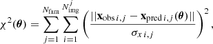 (4)
(4)
where xobs i, j and σx i, j are the observed position of the i-th image of the j-th family and its uncertainty, respectively, and xpred i, j(θ) is the position of the same image as predicted by the model defined by the set of parameter values θ. The accuracy of a given model at reproducing a given set of multiple images is usually measured with the root mean square difference between their model-predicted and observed positions (indicated as Δrms).
A large sample of multiple images is therefore crucial to increase the number of observational constraints for the determination of the best-fit set of parameters. The SL model of MACS J0416 presented in B23 is based on the largest sample of spectroscopically confirmed multiple images ever built for such scope: 237 multiple images from 88 background sources in the redshift range z = 0.94 − 6.63. The best-fit model has Δrms = 0.43″ and includes 213 cluster members. The SL model of MACS J1206 from B19, on the other hand, includes 82 multiple images from 27 background sources in the redshift range z = 1.01 − 6.01. The best-fit model has Δrms = 0.46″ and includes 258 cluster members. The values of Δrms found by B23 and B19 summarised in Table 1, are significantly higher than the astrometric uncertainty on the positions of multiple images (typically smaller than 0.01″). They are however in line with the state of the art of parametric SL models of massive clusters: in spite of the availability of exquisite samples of spectroscopic multiple images, models are still affected by systematics that have an impact on their predicted image positions, such as the choice of the parametrisation of the cluster total mass distribution and the lensing effects of the cluster environment (Meneghetti et al. 2017; Acebron et al. 2017; Grillo et al. 2016; Johnson & Sharon 2016). For instance, as found by Chirivì et al. (2018), the line-of-sight mass distribution of MACS J0416, which is not included in B23, has a significant impact on the reconstruction of the multiple images, although its inclusion is not sufficient to reconcile observations and model predictions. Galaxy-scale SL models are not as affected by intrinsic systematics: we need to fully propagate the uncertainty impacting the cluster-scale mass distribution on the determination of the galaxy-scale parameters.
Reference lensing models of MACS J0416 (B23) and MACS J1206 (B19): relevant parameters.
2.1. Modelling the mass distribution of the cluster members
As described in the previous sub-sections, the cluster members of MACS J0416 and MACS J1206 were modelled with spherical dPIEs with a vanishing core radius. Their total mass only depends on two parameters: their velocity dispersion parameter σ, and their truncation radius rt. In the case of a vanishing core radius, the velocity dispersion parameter σ of a dPIE profile, defined in Eq. (2), is well approximated by the measured stellar central velocity dispersion σ0 (B19). In order to reduce the number of free parameters during the model optimisation, power-law scaling relations were calibrated between the two free parameters and the total luminosity of the cluster members. These relations are usually expressed as
 (5)
(5)
 (6)
(6)
where L0 is the luminosity of the BCG. Cluster-scale SL models are mostly sensitive to the total mass of the cluster members, rather than to the way it is distributed on the scale of the single galaxy, determining a clear degeneracy between σ and rt.
An important step forward in the reduction of the impact of this degeneracy has been driven by the MUSE integral-field spectroscopy, which allows for the measurement of the velocity dispersion of several cluster members, thus obtaining an independent (i.e. not related to the SL constraints) observational prior on the values of α and σref, the slope and the normalisation of the first scaling law presented in Eq. (5); (also known as the Faber-Jackson law, Faber & Jackson 1976). Respectively 64 and 58 measured velocity dispersions have been included in the SL models of MACS J0416 and MACS J1206. This procedure partly breaks the degeneracy between the two parameters describing the cluster members. Using the SL forward modelling code GravityFM (Bergamini et al., in prep.), B23 reconstructed the original surface brightness profile of some sources lensed by MACS J0416 and then traced back their images to the lens plane. They showed that, despite the parametric degeneracies involved, SL models can faithfully reproduce the observed morphology of the GGSL images, and that the accuracy of the reconstruction is enhanced by the inclusion of a larger sample of observed multiple images as a constraint for the optimisation of the model. The degeneracy between the values of the velocity dispersion and of the truncation radius of the cluster members has also been addressed by G22 by replacing the Faber-Jackson law from Eq. (5) with a newly-calibrated FP, a more complex scaling law of which the Faber-Jackson is a projection. This allowed to estimate the central velocity dispersion for all the cluster members included in the model from their observed magnitude and half-light radius.
The σ − rt degeneracy has a very significant impact on the estimate of the compactness of the cluster members. The same total mass value for the cluster members can be obtained with different combinations of the two parameters resulting in a more (or less) compact mass distribution. On the other hand, in a GGSL system, the positions of the multiple images are stringent constraints on the critical lines around the lens galaxies, which strongly depend on its compactness, thus breaking the degeneracy.
3. The galaxy-galaxy strong lensing systems
In this section, we lay out the structure of the three GGSL systems on which we focus our work, the data available for the cluster members, and the procedure followed to obtain the multiple image identification which we later adopt in our lensing analyses.
3.1. MACS J0416.1−2403 ID14
The source ID14, studied in detail by Vanzella et al. (2017), is composed of a pair of faint, young, and compact stellar systems. It has been included in B23 with a spectroscopic redshift of z = 3.221 (Balestra et al. 2016). It is split by the gravitational potential of MACS J0416 into three images separated by up to 50″. One of the three images, shown in Fig. 1, falls close to a pair of elliptical cluster galaxies (members 8971 and 8980 in the reference SL model) and is further split into four images. Following Vanzella et al. (2017), we refer to the two sources as 1 and 2, and to the four images as a, b, c, and d. Knots 1 and 2 have a very similar magnitude in images a and b. Image 1c is the brightest observed, while 2c is much fainter and its position is hard to measure precisely. A detailed photometric study of the lensing system has been performed to build the most recent lensing models: we therefore adopted the positions thereby reported for the images a, b, and c. As such, we also chose to consider 2c in the same position as 1c for the purpose of SL modelling, with a larger uncertainty on its value. In the case of image d, unlike B23, where only image 1d was included in the model, we identified the two components of the source and measured their positions separately. The adopted multiple-image positions are reported in Table 2.
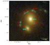 |
Fig. 1. Hubble Frontier Fields RGB image of MACS J0416.1−2403 ID14. The two cluster members are identified as in B23. The two components of the source are identified as 1 and 2. The four multiple images are indicated with the letters a, b, c, and d. |
Multiple image positions for the GGSL system MACS J0416 ID14.
3.2. MACS J0416.1−2403 ID16
The double source identified as ID16 in Bergamini et al. (2021), at a spectroscopic redshift of z = 2.095 (Balestra et al. 2016), is split into three multiple images by the gravitational potential of the cluster main halo. One of the three images falls very close to a pair of elliptical cluster members (8785 and 9129 in the reference SL model, see Fig. 2). The light distribution in the bluest of the HFF bands (ACS F435W) suggests that two further multiple images might fall very close to the centre of cluster member 8785, one of them being almost completely superimposed to it. In order to correctly measure the position of this image and include it in our lensing model, we therefore separated its light from that of the cluster galaxy. We did this in the HFF ACS F606W band, in which both the cluster member and the multiple image are visible. To perform this task, first, we masked the light from the lensed image. The masked pixels are determined in the HST F435W band (where ID16 is less affected by the light of the cluster member). This way, we could run GALFIT (Peng et al. 2010) on the masked F606W image to model the light of the cluster member and measure its structural parameters. In the GALFIT run, the position of the cluster member and its Sérsic index n = 0.5 (Gaussian light distribution) were kept fixed. Parameters such as the magnitude and the half-light radius of the cluster member were manually tuned and fixed to minimise the residual image obtained after its subtraction. No significant over- or under-subtraction regions were observed in the residual image and the residual values are less than 20% of the original image value in every pixel. We therefore used the residual F606W image to measure the positions of all the multiple images, determining their x and y coordinates with Gaussian fits of the light profile. We refer to the two sources as 1 and 2 and to the three images produced by the cluster member 8785 as c, d, and e. We also included image b in the model, which is only at a distance of around 1″ from the cluster galaxy, and for which we have also measured the positions of the two components. The two sources are not clearly resolved in images d and e: we only included the brightest source, identified as 2, in our model. In Fig. 3, we confirm the new identification of two additional multiple images using the reference cluster-scale SL model. Even when only images a, b, and c are included in the optimisation process, the critical lines close to cluster member 8785 create images d and e. As shown in B23, SL forward modelling of the source ID16 performed with GravityFM allows us to very accurately reproduce the observed multiple image configuration and surface brightness distribution. As such, our new multiple image catalogue, presented in Table 3, has been adopted by B23.
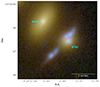 |
Fig. 2. Hubble Frontier Fields RGB image of MACS J0416.1−2403 ID16. The two cluster members are identified as in B23. |
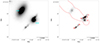 |
Fig. 3. Hubble Frontier Fields imaging of MACS J0416.1−2403 ID16. Left panel: the two cluster members in the ACS F814W band. Right panel: the multiple images in the ACS F435W band. The two components of the source are identified as 1 and 2. The four multiple images are indicated with the letters b, c, d, and e. The critical lines predicted by the model by B23 for a source at redshift z = 2.095 (the same as ID16) are marked in red. |
Multiple image positions determined from HFF photometry for the GGSL system MACS J0416 ID16.
3.3. MACS J1206.2−0847 ID14
The double source ID14 was first included by Grillo et al. (2014) in a similar galaxy-scale lensing study, before a cluster-scale lensing model for MACS J1206 was available. It is treated by B19 as a single source, with a spectroscopic redshift of z = 3.753 (Biviano et al. 2013; Caminha et al. 2017b). Five multiple images are observed, three of them very close to the centre of a cluster member (ID 3910), on which we focus our attention. Their positions are also influenced by the deflection caused by the second brightest cluster member (ID 2541). We refer to the two sources as 1 and 2 and to the three images as a, b, and c, as shown in Fig. 4. We measured their x and y positions, reported in Table 4, using CLASH photometry in the ACS F435W band.
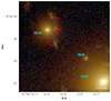 |
Fig. 4. CLASH RGB image of MACS J1206.2−0847 ID14. The two cluster members are identified as in B19. The two components of the source are identified as 1 and 2. The three multiple images are indicated with the letters a, b, and c. |
Multiple image positions determined from CLASH photometry for the GGSL system MACS J1206 ID14.
4. Strong lensing modelling
Our main aim is to use galaxy-scale SL modelling to directly constrain the compactness of the cluster members, and to compare our results with those obtained with cluster-scale modelling, to study their effectiveness at recovering the mass distribution of the cluster sub-structures. In previous galaxy-scale SL studies in clusters (e.g. Grillo et al. 2014; Parry et al. 2016), a simplified description of the cluster-scale mass distribution was included in the SL models to account for its effects on the image deflection. An incorrect determination of the cluster-scale mass distribution can significantly hinder the description of galaxy-scale lenses, especially as far as their azimuthal structure is concerned. In our case, instead, the cluster-scale mass distribution is constrained with accuracy, owing to SL models based on up to more than 200 multiple images of background sources.
In SL models of massive galaxy clusters, the diffuse and galaxy-scale mass components are jointly optimised with the same set of constraints, as described in Sect. 2. The cluster-scale DM haloes dominate the total mass budget and determine the position of its primary critical lines, therefore the parameters that describe their mass distribution have the largest impact on the positions of the multiple images (Meneghetti et al. 2017; Limousin et al. 2022). In addition, the scaling laws connecting the parameters adopted to model the cluster galaxies are mostly influenced by the properties of the most massive members, and power-laws can be too simple to describe the wide mass and morphology range of the cluster members (see G22, Beauchesne et al. 2023). The total mass distribution of the low- and intermediate-mass cluster galaxies is therefore not entirely constrained by cluster-scale SL models, as shown by the difference between the results obtained by describing them with different scaling laws (G22). When modelling a galaxy-scale lens, we thus only optimised the parameters defining the cluster galaxies whose mass distribution significantly impacts the positions of the multiple images, keeping fixed the mass distribution of the rest of the galaxy cluster. To build the χ2 function driving the parametric optimisation (see Sect. 2), we only included the multiple images close to the main galaxy-scale lens (within 2″ from its centre). More distant multiple images could provide us with additional constraints the position of the source, but their position is primarily determined by the mass distribution of other cluster mass components, whose description is subject to a higher uncertainty compared to the determination of the mass profile of the galaxy-scale lens. As such, their inclusion may propagate systematics affecting the total cluster mass onto the determination of the galaxy-scale mass distribution.
To account for this uncertainty on the cluster mass distribution, we did not limit ourselves to considering the best-fit mass models, which may be affected by a systematic bias in the studied region. Instead, we extracted 100 random sets of parameter values from the Markov chain Monte Carlo (MCMC) sampling of the posterior probability distribution of the reference cluster-scale SL model. We then fixed the mass distribution of the cluster-scale components and of all the other members to one of the 100 realisations thus obtained, and optimised the galaxy-scale lenses. We repeated the optimisation for each of the 100 mass models of the cluster. This bootstrapping procedure also allowed us to estimate the uncertainty on the determination of the parameters of the galaxy-scale lenses, and the degeneracies between them. Similarly to the reference models, we modelled the main lens galaxy of each galaxy-scale SL system as a spherical truncated dPIE. We also tested an elliptical non-truncated dPIE mass distribution to understand whether the preference for truncated models could arise from the insufficient azimuthal complexity of the spherical total mass model adopted. We performed all SL optimisations using LensTool.
4.1. MACS J0416.1−2403 member galaxy 8971
The galaxy-scale SL system MACS J0416 ID14 was described in Sect. 3.1. Throughout the SL modelling procedure we adopted the multiple image catalogue presented in Table 2, comprising of eight multiple images from two background sources. All of the multiple images of the source ID14 are observed close to the cluster member 8971 (hereafter member 8971), at an average angular distance of 1.07″: we thus focused on constraining its truncation radius. Cluster member 8980 significantly influences the multiple-image configuration, so we also optimised its mass distribution.
In B23, member 8971 was not included in the scaling relations adopted to describe the remaining cluster members, and it was modelled separately as a truncated dPIE profile. The values of the parameters of its total mass distribution are reported in Table 5, with an uncertainty provided by the MCMC sampling of their marginalised posterior probability distribution. The ellipticity of the halo converges to the upper limit of its prior, indicating that it is poorly constrained and perhaps compensates for some unaccounted shear.
Best-fit values and 1σ errors of the parameters describing the cluster member 8971 in the SL model of MACS J0416 by B23.
As anticipated, we first described member 8971 as a spherical truncated dPIE with vanishing core (hereafter SISt), whose centre is fixed at the light centre. The two free parameters are thus the velocity dispersion σ2 and the truncation radius rt. The alternative model, an elliptical non-truncated dPIE with a vanishing core (hereafter SIE), has three free parameters in σ, the ellipticity e3, and the orientation angle θe4. As we wish to focus on studying the radial structure of member 8971, we considered simpler models for the mass distribution of the cluster member 8980. We tested spherical truncated and non-truncated isothermal models, and we noticed some degeneracy between the value of rt for member 8980 and the parameters describing member 8971. To avoid this, we chose to describe member 8980 with a SIS mass profile.
We optimised the two galaxy-scale SL models that we just outlined (with member 8971 parametrised as a SISt and a SIE respectively) for each of the 100 cluster-scale total mass distribution realisations obtained as described earlier. With this bootstrapping procedure, we obtained a set of 100 best-fit values for the parameters of the galaxy-scale SL system: we used the median, the 16th, and the 84th percentiles of the resulting distribution of best-fit values to obtain an estimate of their value and its uncertainty. Studying the marginalised distribution of the 100 best-fit parameters also provides us with insights on the degeneracy between them. Unlike in B23, where LensTool struggled to recover rt and the ellipticity of member 8971 at the same time, all the parameters of the SISt and SIE models are well constrained, with a low uncertainty. Their values are reported in Table 6. In the case of the SISt mass profile, the total mass can be obtained as
 (7)
(7)
Best-fit values and 1σ errors of the parameters of our galaxy-scale SL models of MACS J0416 ID14.
We can thus estimate a total mass value of  for 8971.
For each best-fit model, we estimate the value of Δrms, and we refer to the average value of Δrms obtained for the 100 realisations of the model as ⟨Δrms⟩: we find ⟨Δrms⟩ = 0.08″ for the SISt models and 0.04″ for the SIE model. We note that the SIE model allows for lower values of Δrms, which might be due to having one additional parameter compared to the SISt model. This may imply that a spherical mass distribution is too simple to describe the total mass distribution in the region, perhaps also due to unaccounted shear from the cluster-scale mass distribution. This is also suggested by the high value of ellipticity reported by B23.
Given the significant difference in the best-fit value of σ between the models, we compare them with the measured stellar line-of-sight velocity dispersion (LOSVD) for member 8971. The NE region of MACS J0416 was included in the MUSE Deep Lens Field Vanzella et al. (2021), a very deep (17.1 h integration time) MUSE observation with a seeing of approximately 0.6″. The value of σ recovered by SL models is a central three-dimensional mass density scale, while the value of LOSVD is a projected stellar velocity dispersion, which depends on the light distribution and on the point spread function of the observations, so the two values do not need to be exactly identical. We extracted the spectrum of member 8971 within a circular aperture centred in the centre of light of the galaxy and with a radius equal to the seeing of 0.6″, to probe the central regions of the cluster galaxy. We measured the LOSVD using pPXF (penalised pixel-fitting) by Cappellari & Emsellem (2004) and Cappellari (2017, 2023), comparing the observed spectra with a set of 463 UVB stellar templates from the X-shooter Spectral Library (XSL) DR2 (Gonneau et al. 2020) with a signal-to-noise ratio (S/N) greater than 100 Å−1, combined and convolved with a LOSVD. The fit, whose results are shown in Fig. 5, minimises a χ2 function between the observed spectrum and a model and provides a measured LOSVD value of 178.0 ± 2.4 km s−1, for an average S/N value of 64.6 over the spectrum. The very low error on the measured value only includes the statistical uncertainty of the final LOSVD fit and does not include possible systematics introduced by the choice of the stellar templates adopted to fit the spectrum. The velocity dispersion value found by our SISt galaxy-scale SL model is consistent within approximately 2σ with the measured LOSVD. The comparison with the value found by our SIE model is less straightforward due to the change in the surface area within a given iso-density contour at a fixed σ determined by the introduction of the ellipticity through transformation defined in Eq. (3). However, we note that our ellipticity value of e = 0.18 implies a change in iso-density areas of only 1% with respect to the spherical case, which allows us to compare the two values in first approximation. While the SL and the kinematic estimates of σ do not probe exactly the same physical quantity, we would expect them to have similar values, and only our SISt model seems to allow for that. This comparison is not performed in the following sections for members 8785 and 3910, whose spectra have low S/N values, probably due to a very faint lens magnitude and a lower MUSE exposure time, respectively. The determination of the S/N threshold for a reliable LOSVD measurement requires further tests and larger samples, and will be presented in an upcoming work (Granata et al., in prep.). The predicted compactness of the cluster galaxy 8971 and the evidence for a truncated total mass density profile are discussed in Sect. 5.
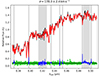 |
Fig. 5. Fitting of the LOSVD of the MUSE spectrum of member 8971 with pPXF. The observed spectrum is shown in black, the red curve is the best-fit model, while the green points show the difference between the data and the model. The blue shaded regions along the wavelength axis were excluded in the fitting procedure, due to the presence of sky subtractions around emission lines or laser lines in the spectrum. |
4.2. MACS J0416.1−2403 member galaxy 8785
The galaxy-scale SL system MACS J0416 ID16 was described in Sect. 3.2. Throughout the SL modelling procedure we adopted our new multiple image catalogue, presented in Table 3 and comprising of six multiple images from two background sources. All six of the multiple images of the source ID16 are observed close to the cluster member 8785 (hereafter member 8785), at an average angular distance of only 0.43″ from its centre. We thus focused on constraining the truncation radius of member 8785, and optimised the mass distribution of member 9129, which significantly influences the multiple-images configuration, as well.
In B23, member 8785 was modelled using the scaling relations (Eqs. (5) and (6)) leading to a velocity dispersion value 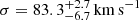 and a truncation radius
  , resulting in a total mass
 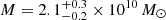 . We first described member 8785 as a SISt, and we studied an alternative SIE model. Again, we tested several models for member 9129, and we chose a SIS mass profile to avoid degeneracies between parameters.
We ran the SISt and SIE models for each of the 100 cluster-scale total mass distributions extracted from the MCMCs. In Table 7, we present the results of our bootstrapping procedure: the median values of the parameters of the best-fit galaxy-scale lensing models, and the 1σ uncertainties derived from their 16th and 84th percentiles.
Best-fit values and 1σ errors of the parameters of our galaxy-scale SL models of MACS J0416 ID16.
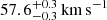
The offsets between the observed and model-predicted positions of the multiple images are extremely small, with a value of ⟨Δrms⟩, the average of Δrms for the 100 model realisations, of 0.01″ for both the SISt and the SIE models. This value is lower than the observational uncertainty on the determination of the positions of the multiple images. The distribution of the best-fit values of the free parameters, for the 100 cluster-scale mass distributions we consider, suggests that they are well constrained, with a low uncertainty and without clear degeneracies between them. Comparing our results for the SISt model with those from B23, we find lower values for σ and rt, corresponding to a lower total mass value of  . This discrepancy may be due to a bias introduced by the scaling relations adopted in B23: cluster-scale SL models that describe the sub-halo component with the FP find that power-law scaling relations can over-predict the total mass (G22) and the velocity dispersion (Beauchesne et al. 2023) of low- and intermediate-mass cluster galaxies. In Sect. 5, we discuss the inferred compactness of member 8785.
4.3. MACS J1206.2−0847 member galaxy 3910
The galaxy-scale SL system MACS J1206 ID14 was described in Sect. 3.3. Throughout the SL modelling procedure we adopted our new multiple image catalogue, presented in Table 4 and comprising of six multiple images from two background sources. All six of the multiple images of the source ID14 are observed close to the cluster member 3910 (hereafter member 3910), at an average angular distance of 1.11″ from its centre: we thus focused on constraining its truncation radius. Cluster member 2541, at a distance of 6.86″ from the centre of 3910, is the second brightest cluster galaxy, with a predicted total mass of 9.55 × 10¹¹ M⊙ in B19. Closer to 3910 is the low-mass (M = 1.97 × 10⁹ M⊙) cluster member 3920. Due to its high total mass, we optimised the mass distribution of cluster member 2541 as well, whereas we kept the parameters describing 3920 fixed to the values predicted by cluster-scale modelling.
Member 3910 was described by B19 with the two scaling relations (Eqs. (5) and (6)), leading to best-fit values of the velocity dispersion and of the truncation radius of 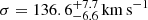 and
and 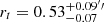 , for a total mass
 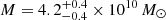 . Again, we first described 3910 as a SISt, and we tested an alternative SIE model. With regards to cluster member 2541, we note that in this case we are able to constrain its truncation radius without unforeseen parametric degeneracies, and thus we adopted a SISt model.
We ran the SISt and SIE models for each of the 100 cluster-scale total mass distributions extracted from the MCMCs. In Table 8, we present the median values of the parameters of the best-fit galaxy-scale lensing models, as derived from the bootstrapping procedure, with 1σ uncertainty derived from their 16th and 84th percentiles.
Best-fit values and 1σ errors of the parameters of our galaxy-scale SL models of MACS J1206 ID14.
As in the case of MACS J0416 ID16, we find very small offsets between the observed and predicted multiple images, with an average Δrms value of ⟨Δrms⟩ = 0.01″ for the SISt model and 0.03″ for the SIE model. In spite of having fewer free parameters, the SISt model allows for a more accurate reconstruction of the lensing observables, and all parameters are estimated with a low statistical uncertainty, as clear from Table 8. On the other hand, the SIE model cannot constrain well the value of the velocity dispersion of member 2540, which tends to the upper limit of our prior, and the predicted ellipticity of member 3910 is very high5, suggesting that it might be needed to compensate for the lack of truncation in the total mass profile. Comparing our SISt model with B19, we find lower values for σ and significantly higher values for rt, for a total mass value of  , higher than the best-fit value from B19. Again, the Faber-Jackson law adopted by B19 may be biasing the value of σ and therefore of the truncation radius. Grillo et al. (2014) use a one-parameter SIS mass profile to describe the cluster member, finding σ = 97 ± 3 km s−1. The lower value of σ is expected, given the lack of a truncation of the mass profile. In the next section, we perform a more meaningful comparison, looking at the mass value within the effective radius.
5. Analysis and discussion
5.1. Truncation radius of the cluster members
As detailed in the previous section, our galaxy-scale SL modelling procedure was aimed at estimating the truncation radius of three lens galaxies in massive clusters. The recovered values of rt for members 8971, 8785, and 3910 are  ,
,  , and
, and  , respectively. To better illustrate the radial scales at play, we built a cumulative total mass profile of the three members by comparing the 100 best-fit mass profiles obtained with the bootstrapping procedure and by taking the 50th percentile at each projected radius. We also estimated the statistical uncertainty on the total mass profile from the 16th and 84th percentiles. We performed the same procedure on the SL models of the three cluster members by B23 and B19, using their MCMC sampling of the parametric posterior probability distribution to quantify the uncertainty on their total mass distributions. These profiles are shown in Fig. 6. We note that this procedure only accounts for the statistical uncertainty on the mass distribution parameters, and not for the possible systematics.
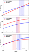 |
Fig. 6. Projected cumulative total mass profiles for the lens galaxies studied in this work compared with the predictions of B23 and B19. From the top to the bottom panel: member 8971, member 8785, and member 3910. The vertical bars indicate the inferred values of the truncation radius. Shaded regions indicate the 16th and 84th percentiles for the mass profile and the truncation radius. The projected distances of the observed multiple images from the lens centre are marked with vertical black lines. |
As shown in Figs. 6 and 7, the measured values of the truncation radius are, for all three members, within the range of the observed positions of the multiple images. In this radial range, SL allows for the highest accuracy in the reconstruction of the total mass profile of a lens, and is therefore more sensitive to its slope. In all three cases, we have tested an alternative non-truncated SIE mass parametrisation to inquire whether the truncated profile could actually be compensating for an insufficient description of the lens azimuthal structure. Despite having 4 free parameters, as opposed to the 3 of the SISt model, only in one of the three cases (member 8971), the SIE model leads to a slightly lower value of Δrms. In one case (member 3910), the SIE model predicts a very high value of the lens ellipticity, which is not suggested by the light distribution. In conclusion, in all three systems we find that a spherical truncated total mass distribution for the lens galaxy is able to reproduce the SL observations with a small Δrms and provide the value of rt with a low statistical error. In two out of the three cases, a non-truncated model with a higher number of parameters does not improve the description of the system, in one case leading to unrealistic parameter values.
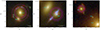 |
Fig. 7. Truncation radius of members 8971, 8785, and 3910 superimposed to the RGB cutout of the respective galaxy-scale SL system. We show the best fit value as a solid line and the 1σ uncertainty range with dashed lines. |
Suyu & Halkola (2010) performed a similar truncation radius measurement for a satellite galaxy (z = 0.351) of the massive elliptical lens SL2S J08544−0121, which influences the shape of an Einstein ring determined by the main lens. They find a value of rt close to its theoretically predicted tidal radius. Figure 8 shows that the value of rt estimated in Suyu & Halkola (2010) seems to agree with the σ-to-rt relation found in our work. Monna et al. (2015) repeated the procedure for the CLASH-VLT galaxy cluster Abell 383. They combined SL with observational priors on the observed velocity dispersion for two high mass (total mass greater than 1012 M⊙) members close to two lensed arcs of the same sources. The recovered value of rt is greater than 50 kpc for both galaxies, significantly higher than predicted by the scaling law calibrated for the other cluster members of Abell 383. The authors suggest that very bright members may have not undergone strong stripping as a result of being a central galaxies prior to accretion on the cluster. Both Suyu & Halkola (2010) and Monna et al. (2015) based their SL modelling procedure on surface brightness reconstruction of extended arcs, finding that this significantly improves the accuracy of the constraints on the value of the truncation radius. In this work, we only used the centroid position of the multiple images, rather than their full surface brightness. However, unlike in Suyu & Halkola (2010) and Monna et al. (2015), the cluster-scale mass distribution determines several different multiple images of the background source close to the galaxy-scale lens, rather than a single extended lensed arc. In our case, several multiple images are observed at different projected distances from the lens centre, providing us with detailed information about the galaxy total mass profile and its slope.
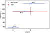 |
Fig. 8. Relation between the values of the velocity dispersion and of the truncation radius for the three cluster members included in this study (in blue) and for a satellite of SL2S J08544−0121, as measured by Suyu & Halkola (2010; in red). The inferred uncertainty on the velocity dispersion of member 8785 is too small to be visible in this plot. |
Finally, we tested whether the inferred values of rt may be biased by the parametrisation chosen by B23 and B19 for the total mass profile of the haloes included in the model. To do so, we built an alternative cluster-scale model for MACS J1206 in which all of the cluster members are described with singular isothermal sphere (SIS) mass profiles (i.e. with infinite rt) and repeated the statistical analysis described above. We find that this does not influence significantly the estimated parameter values for the lens galaxy 3910, suggesting that our modelling procedure is robust with respect to the parametrisation choices adopted for the remaining cluster mass components.
5.2. Compactness of the cluster galaxies
Galaxy-scale SL events in massive clusters allowed us to infer the physical properties of some selected cluster galaxies without relying on the scaling laws typically adopted to describe them. Cluster-scale SL modelling is mostly sensitive to the total mass of the cluster galaxies, rather than to the details of their mass density profiles. As such, σ and rt suffer from a strong degeneracy and cannot be separately constrained in absence of an observational prior: this significantly limits the insights on the compactness of the cluster galaxies. To break the degeneracy between σ and rt, B19 and B23 obtained a kinematic prior on the value of the slope of the Faber-Jackson law (marked as α in Eq. (5)). Assuming a total mass-to-light ratio M/L ∝ Lγ leads to β = γ − 2α + 1 (β is defined in Eq. (6)). From Eq. (7), one can then derive a total mass-to-σ scaling law
 (8)
(8)
B19 and B23 assumed γ = 0.2, as suggested by the FP. The reference values of the scaling laws (σref and  in Eqs. (5) and (6)) are mostly determined by the high-mass cluster members, which have a stronger influence on the positions of the observed multiple images. On the other hand, once γ is fixed, the value of α fixes the slopes of the two laws, determining the description of the total mass distribution of the low- and intermediate-mass cluster members.
Considering the reference sample of clusters included in Meneghetti et al. (2020), B19 find  for MACS J1206 and
  for AS1063, while Bergamini et al. (2021) and B23 find
  for MACS J0416, corresponding to M ∝ σ4.3, M ∝ σ4.4, and M ∝ σ4.0, respectively. The same procedure was adopted by Bergamini et al. (2023b) for the HFF cluster Abell 2744 (A2744), finding a value of
  (implying M ∝ σ3.0). In the top panel of Fig. 9, we compare the M-to-σ scaling law for these four cluster scale SL models with the values of total mass and velocity dispersion for the galaxy-scale SL systems. In cluster-scale models, only the values σref and
  are optimised: we estimated the uncertainty on the determination of the M-to-σ relation based on the MCMC sampling of the posterior probability distribution for these two parameters. We notice that the scaling relations used in cluster-scale models have significantly different normalisation and slope values. In particular, the SL model of MACS J0416 consistently predicts higher mass values at a fixed σ compared to those of MACS J1206 and AS1063. On the other hand, the model of A2744 has a significantly lower slope, predicting higher total mass values at low σ. Looking at the three cluster members studied in this work, only the M-to-σ relation found for A2744 seems to represent well their compactness.
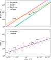 |
Fig. 9. Comparison between the M-to-σ relation estimated by our analysis and those adopted for the cluster galaxies in the SL models of MACS J0416 (B23), AS1063 (B19; G22), MACS J1206 (B19), and A2744 (Bergamini et al. 2023b). Top panel: comparison with the SL models describing the cluster galaxies according to Eqs. (5) and (6). Bottom panel: comparison with the SL model of AS1063 by G22, based on the FP. |
In the SL model of AS1063 by G22, the values of σ were fixed from the observed luminosity and half-light radius Re of the cluster galaxies, while a proportionality law was calibrated between the observed Re and rt. As such, the M-to-σ relation is not a power-law and is able to include a realistic scatter. As shown by the bottom panel of Fig. 9, the relation significantly differs from those obtained with a power-law approach: a bi-logarithmic fit of the relation predicts a slope of 2.0. The panel also shows that the three galaxy-scale lenses that we have modelled in this work lie within the scatter of the scaling relation derived by G22 using the FP. While a sample of three objects is very small, it is interesting to note that the M-to-σ relation for the galaxy scale lenses, derived exclusively with SL, is very close to the predictions of G22, where lensing observables are only used to estimate the ratio between Re and rt. A more complex description of the cluster galaxies based on the FP leads to inferred properties which are compatible with our analysis. Beauchesne et al. (2023) recently modelled AS1063 adopting an intermediate approach between B19 and G22, where galaxies are described with the Faber Jackson law or the FP depending on the observations available for them. The value of α was optimised together with the parameters of the FP to avoid inconsistent slopes. Choosing γ = 0, they find α = 0.34, obtaining to M ∝ σ3. On the other hand, fixed power-law scaling relations do not seem to be able to correctly describe the spatial structure of the cluster galaxies on the whole mass range included in SL models. As shown by Fig. 6, we predict significantly different properties for members 8785 and 3910 compared to B23 and B19: the former has a similar value of rt but a higher σ, while the latter has a significantly larger rt.
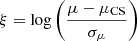
These differences may have a non-negligible impact on the magnification factor predicted close to the galaxy-scale lenses, which connects the observed and the unlensed magnitude for the multiply imaged sources. We measured the magnification predicted by the three galaxy-scale models. For each of them, we used the 100 models from our boot-strapping procedure to estimate the uncertainty on the magnitude value. In Fig. 10, we map the value of  , where μ is the magnification predicted by our models, σμ is the uncertainty on its value, and μCS is the magnification from the cluster-scale models (by B23 and B19). The upper panel of Fig. 10 shows that our work and B23 predict significantly different magnifications close to member 8971. However, these differences are probably due to the different mass parametrisation chosen by the two models and are less pronounced close to the positions of the multiple images, where the total mass distribution is better constrained. As expected, close to members 8785 and 3910, the value of ξ is closer to zero as a consequence of choosing the same mass parametrisation in the two models. In all three cases, with few exceptions, the difference between the predicted values of the magnification is relatively small close to the multiple images, where the total mass distribution of the lens is better reconstructed. In conclusion, the systematics related to the mass modelling of the cluster members affect the predicted magnification map of lens clusters close to member galaxies. These predictions are more robust in proximity of the observed positions of the multiple images, but a more realistic description of the total mass properties of lens galaxies can benefit the accuracy of the studies of high-redshift lensed sources.
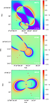 |
Fig. 10. Comparison between the magnification values close to the three galaxy-scale lenses predicted in this work and in B23 and B19. The colour map is based on the value of |
5.3. Comparison with cosmological simulations
In this sub-section, we compare the compactness of the cluster members as obtained from our galaxy-scale SL models with the theoretical predictions of cosmological simulations. This study offers an excellent opportunity to contrast the properties of observed and simulated galaxy-scale lenses in massive clusters (although we note that member 8785 is not the main lens responsible for the secondary critical line that produces system ID16). As in Meneghetti et al. (2020), we adopt the maximum circular velocity of the cluster members, defined as
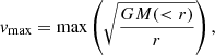 (9)
(9)
where  for an isothermal model, as a proxy for the compactness of cluster galaxies (see Meneghetti et al. 2020, 2022, 2023; Ragagnin et al. 2022): more compact objects have higher values of vmax at a fixed total mass. In Fig. 11, we compare the vmax-to-M relation for our work with those found in Ragagnin et al. (2022) for a set of zoom-in re-simulations of the Dianoga suite (Planelles et al. 2014; Rasia et al. 2015) of simulated galaxy clusters. These setups differ from one another in terms of their softening and feedback schemes. As in Ragagnin et al. (2022), we refer to the three models considered as R15 (presented in Rasia et al. 2015), RF18 (presented in Ragone-Figueroa et al. 2018), and B20 (presented in Bassini et al. 2020). The setups are also referred to as 1x or 10x if they have the same mass resolution as the Dianoga suite, or a ten times lower particle mass, respectively.
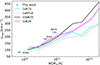 |
Fig. 11. Comparison between the vmax-to-M relation obtained from our analysis and those predicted by the cosmological hydrodynamical simulations described in Ragagnin et al. (2022). The naming convention for the different suites is presented in the text. |
Figure 11 shows that members 8971 and 3910 both have a maximum circular velocity value higher than those for simulated sub-haloes with the same total mass, irrespective of the feedback scheme or the resolution considered in Ragagnin et al. (2022), indicating a level of compactness higher than that predicted by simulations. This seems to suggest that the discrepancy between SL models and simulations cannot be entirely ascribed to systematics affecting the former, as a result of the adoption of power-law scaling relations to describe the cluster members, as noted already by G22. Member 8785 falls in a total mass range (M < 1010 M⊙) which was excluded from the analyses of Meneghetti et al. (2020), because the current cosmological simulations do not have enough mass resolution.
5.4. Stellar mass of the cluster members
In this sub-section, we study the stellar-to-total mass fraction of the cluster members. Measuring its value within the effective radius is an important probe of the interplay between the effects of the baryonic feedback processes and the gravitational potential of DM during galaxy formation (see Shajib et al. 2022; Smith 2020), and of stellar populations in early-type galaxies. These processes are particularly significant for lower-mass galaxies, which should have a higher stellar-to-total mass fraction compared to the very massive early-type galaxies that dominate the samples of lens galaxies. Our work significantly extends the typical mass range of current studies, similarly to what will be performed with the upcoming samples of galaxy-scale lenses unveiled by Euclid and LSST.
The values of the total stellar mass of the three lens galaxies have been measured in recent works. For members 8971 and 8785, we followed the best-fit relation between the stellar mass and the magnitude in the HST F160W band found by Grillo et al. (2015), log(M*(M⊙)) = 18.541 − 0.416 × F160W, where M* is the stellar mass of the cluster member. To consider the scatter about this mean relation, we chose a 40% uncertainty on the derived stellar mass values of (2.4 ± 1.0)×1010 M⊙, and (4.0 ± 1.6)×109 M⊙, respectively. For member 3910, we adopted the value measured by Grillo et al. (2014) of (1.7 ± 1.0)×1010 M⊙. In both cases, the stellar mass measurements were based on the HST spectral energy distribution (SED) of the lens galaxies, using composite stellar population models, and a Salpeter (Salpeter 1955) stellar initial mass function (IMF). In Fig. 12, we show the relation between the stellar mass and the velocity dispersion for the three cluster members studied in this work and for the 85 SLACS lenses presented in Auger et al. (2009), which are representative of the currently known population of lens galaxies. We note that the SLACS lenses were modelled with non-truncated total mass profiles, which could affect the recovered values of the velocity dispersion. The figure showcases the significant extension of the range of stellar mass and velocity dispersion values probed in this work compared to current samples of lens galaxies.
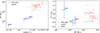 |
Fig. 12. Stellar mass of lens galaxies: comparison between this work and the 85 SLACS lens galaxies presented in Auger et al. (2009). Left panel: Stellar mass as a function of the velocity dispersion. Right panel: Stellar-to-total mass fraction measured within the effective radius; the 68% confidence interval found by Grillo (2010) for a selected sample of 2 × 10⁵ SDSS early-type galaxies is also shown. |
Using GALFIT on the HFF (for MACS J0416) or CLASH (for MACS J1206) F814W band images, we measured the effective radii, Re, of the three galaxies, finding 1.41 ± 0.02 kpc6, 0.77 ± 0.03 kpc, and 2.13 ± 0.09 kpc, respectively. They correspond to a ratio between the truncation and the half-light radius  of 4.3 ± 1.6, 5.13 ± 0.72, and 2.77 ± 0.47, all higher than the average value of 2.3 found by G22 for the cluster members of AS1063, although they fall within the scatter around their mass-to-σ relation. From the total mass profile derived for each of the 100 best-fit models of the three galaxies, we obtained the total mass enclosed within the effective radius M(< Re) and its uncertainty. The stellar-to-total mass fraction within the effective radius for the three members is therefore
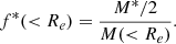 (10)
(10)
We find 0.51 ± 0.21, 1.0 ± 0.4, and 0.39 ± 0.16, for members 8971, 8785, and 3910, respectively.
We compare our values of the stellar-to-total mass fraction as a function of the stellar mass with the analogous relation found for the 85 SLACS lens galaxies presented in Auger et al. (2009; similar results had previously been obtained by Grillo et al. 2008). We take their stellar mass values measured with a Salpeter stellar IMF and the stellar-to-total mass fraction within the effective radius measured in the rest-frame V-band (comparable with the F814W band for the two clusters considered in this work). As clear from Fig. 12, we probe a lower stellar mass range, but find compatible values between the two samples. Our values agree with the results of G22 for the cluster members of AS1063. We also included in Fig. 12 the values found, starting from the same hypotheses, by Grillo (2010) for a selected sample of 2 × 10⁵ SDSS early-type galaxies, which we find to be compatible both with our work and with that by Auger et al. (2009). These results suggest that the tidal truncation to which the three lens galaxies are subject to, by virtue of the dense cluster environment in which they reside, only marginally affects their structure within the effective radius. This is in agreement with the conclusions of Grillo & Gobat (2010), Grillo et al. (2014), Parry et al. (2016), and G22, who compared the stellar fraction within the effective radius of cluster and field early-type galaxies.
6. Conclusions
In this article we have presented the measurement with SL of the truncation radius of three cluster galaxies. We considered the reference sample of galaxy clusters included in the analysis by Meneghetti et al. (2020) and selected galaxy-scale SL systems with a clear morphology and several multiple images close to one or a few member galaxies. We chose to focus on members 8971 and 8785 of MACS J0416, and member 3910 of MACS J1206. We built galaxy-scale SL models for the three cluster members and for the neighbouring galaxies which influence the lensing system the most.
We accounted for the lensing effects of the remaining mass components of the cluster according to the predictions of the most recent and accurate SL models of MACS J0416 and MACS J1206, presented in B23 and B19, respectively. To properly consider the uncertainty on the total mass distribution of the two clusters, we sampled the posterior probability distribution of the parameters of the two models, and extracted 100 points, corresponding to 100 realisations of the cluster-scale mass distribution. For each of them, we optimised the models of the mass distribution of the three galaxy-scale lenses. This bootstrapping procedure allowed us to obtain a realistic estimate of the uncertainty on the lens parameters and of the degeneracy between them. We described the three members on which we focus our analysis with spherical truncated profiles and test alternative ellipsoidal non-truncated models. The main conclusions of our analyses are summarised as follows:
-
We measured a truncation radius value of
 ,
,  , and
, and  for members 8971, 8785, and 3910, respectively. These values correspond to a total mass of
  ,
,  , and
, and 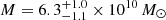 , respectively, and to velocity dispersion values of
 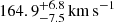 ,
,  , and
, and 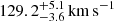 , respectively.
 -
The values of rt are well constrained, with a low statistical uncertainty. We compare our results with those of Suyu & Halkola (2010) for the satellite galaxy of the lensing system SL2S J08544−0121, finding very similar rt values for galaxies in the same total mass range.
-
In the case of member 8971, the SIE model leads to a lower value of Δrms, but the comparison between the SL-derived σ and the measured LOSVD value of 178.0 ± 2.4 km s−1 strongly favours the SISt model.
-
In the other two instances, SIE models do not lead to an improved accuracy of the description of the SL observations, in spite of their more complex azimuthal structure and a higher number of free parameters. In the case of member 3910, the parameters of the non-truncated models are not well constrained and show clear degeneracies.
-
Our inferred values of σ and rt for the three cluster galaxies differ significantly from the results of B23 and B19, especially in the case of members 8785 and 3910, where they were derived with power-law scaling relations with respect to the galaxy total luminosity.
-
We compare our results with the total-mass-to-σ relations for MACS J0416, MACS J1206, AS1063, and A2744 from B23, B19, and Bergamini et al. (2023b), obtained with the power-law approach. We find that the scaling relations cannot consistently describe all three members studied in this work. Our results instead agree with the mass-to-σ relation derived by G22 for AS1063, based on the FP relation and showing a larger scatter.
-
We juxtapose the estimated compactness of the three lens galaxies with the predictions of the hydrodynamical cosmological simulation suites presented in Ragagnin et al. (2022), which differ in feedback and softening scheme, and mass resolution. Members 8971 and 3910 fall in the total mass range included in the analyses performed on the simulations. Their measured compactness is higher than what is found for simulated sub-haloes of the same total mass, independently of the simulation set-up considered, confirming the discrepancy between observations and simulations first reported in Meneghetti et al. (2020).
-
We measured the stellar mass and the effective radius, and the stellar-to-total mass fraction within the effective radius for the three cluster galaxies. For the latter parameter, we find 0.51 ± 0.21, 1.0 ± 0.4, and 0.39 ± 0.16 for members 8971, 8785, and 3910, respectively. Our values span the same range as those observed for the members of AS1063 by G22, for the 85 SLACS lens galaxies presented in Auger et al. (2009), and for a selected sample of early-type SDSS galaxies by Grillo (2010), suggesting that the tidal truncation of cluster galaxies does not significantly affect their structure within the effective radius.
As clear from Fig. 12, our work significantly extends the mass range probed by current SL studies of early-type galaxies, towards the regimes that will be systematically explored by the upcoming lens surveys with the Euclid and the Rubin telescopes. On-going integral-field observations with the James Webb Space Telescope Near Infrared Spectrograph will provide us with spatially resolved kinematic constraints of galaxy-scale lenses in clusters, allowing for a more detailed reconstruction of the mass structure of member galaxies.
Equation (3) implies that, compared to the spherical case, the area enclosed by a given iso-surface-density contour changes by a factor (4ab)(a + b)−2.
Included by LensTool via a fiducial velocity dispersion  .
.
e = (a2 − b2)(a2 + b2)−1, where a and b are the major and minor semi-axes of the ellipse.
Counter clockwise sexagesimal degree between the semi-major axis and the positive x axis on the lens plane.
As such, the value of σ3910 of the SISt model cannot be compared directly to that of the SIE model.
Compatible with the value measured by Tortorelli et al. (2023).
Acknowledgments
We thank the anonymous referee for some useful suggestions that helped us to improve the paper. We acknowledge financial support by PRIN-MIUR 2017WSCC32 (P.I:: P. Rosati), PRIN-MIUR 2020SKSTHZ (P.I.: C. Grillo), INAF main-stream 1.05.01.86.20 (P.I.: M. Nonino) and INAF 1.05.01.86.31 (P.I.: E. Vanzella). M.M. was supported by INAF Grant The Big-Data era of cluster lensing. M.M. also acknowledges support from the Aspen Center for Physics and Simons Foundation. This work uses the following software packages: Lenstool (https://projets.lam.fr/projects/lenstool/wiki; Jullo et al. 2007; Jullo & Kneib 2009), Astropy (https://github.com/astropy/astropy; Astropy Collaboration 2013, 2018), matplotlib (https://github.com/matplotlib/matplotlib; Hunter 2007), NumPy (https://github.com/numpy/numpy; van der Walt et al. 2011; Harris et al. 2020), pPXF (https://pypi.org/project/ppxf/; Cappellari & Emsellem 2004; Cappellari 2023), Python (https://www.python.org/; Van Rossum & Drake 2009), Scipy (https://github.com/scipy/scipy; Virtanen et al. 2020).
References
- Abbott, T. M. C., Allam, S., Andersen, P., et al. 2019, ApJ, 872, L30 [Google Scholar]
- Acebron, A., Jullo, E., Limousin, M., et al. 2017, MNRAS, 470, 1809 [Google Scholar]
- Acebron, A., Grillo, C., Bergamini, P., et al. 2022, A&A, 668, A142 [NASA ADS] [CrossRef] [EDP Sciences] [Google Scholar]
- Annunziatella, M., Bonamigo, M., Grillo, C., et al. 2017, ApJ, 851, 81 [NASA ADS] [CrossRef] [Google Scholar]
- Astropy Collaboration (Robitaille, T. P., et al.) 2013, A&A, 558, A33 [NASA ADS] [CrossRef] [EDP Sciences] [Google Scholar]
- Astropy Collaboration (Price-Whelan, A. M., et al.) 2018, AJ, 156, 123 [Google Scholar]
- Auger, M. W., Treu, T., Bolton, A. S., et al. 2009, ApJ, 705, 1099 [Google Scholar]
- Auger, M. W., Treu, T., Bolton, A. S., et al. 2010, ApJ, 724, 511 [NASA ADS] [CrossRef] [Google Scholar]
- Bacon, R., Accardo, M., Adjali, L., et al. 2010, in Ground-based and Airborne Instrumentation for Astronomy III, eds. I. S. McLean, S. K. Ramsay, & H. Takami, SPIE Conf. Ser., 7735, 773508 [Google Scholar]
- Balestra, I., Mercurio, A., Sartoris, B., et al. 2016, ApJS, 224, 33 [Google Scholar]
- Bassini, L., Rasia, E., Borgani, S., et al. 2020, A&A, 642, A37 [NASA ADS] [CrossRef] [EDP Sciences] [Google Scholar]
- Beauchesne, B., Clément, B., Hibon, P., et al. 2023, MNRAS, in press, https://doi.org/10.1093/mnras/stad3308 [Google Scholar]
- Bender, R., Burstein, D., & Faber, S. M. 1992, ApJ, 399, 462 [NASA ADS] [CrossRef] [Google Scholar]
- Bergamini, P., Rosati, P., Mercurio, A., et al. 2019, A&A, 631, A130 [NASA ADS] [CrossRef] [EDP Sciences] [Google Scholar]
- Bergamini, P., Rosati, P., Vanzella, E., et al. 2021, A&A, 645, A140 [EDP Sciences] [Google Scholar]
- Bergamini, P., Grillo, C., Rosati, P., et al. 2023a, A&A, 674, A79 [NASA ADS] [CrossRef] [EDP Sciences] [Google Scholar]
- Bergamini, P., Acebron, A., Grillo, C., et al. 2023b, A&A, 670, A60 [NASA ADS] [CrossRef] [EDP Sciences] [Google Scholar]
- Biviano, A., Rosati, P., Balestra, I., et al. 2013, A&A, 558, A1 [Google Scholar]
- Bolton, A. S., Burles, S., Koopmans, L. V. E., Treu, T., & Moustakas, L. A. 2006, ApJ, 638, 703 [NASA ADS] [CrossRef] [Google Scholar]
- Bonamigo, M., Grillo, C., Ettori, S., et al. 2018, ApJ, 864, 98 [Google Scholar]
- Borgani, S., & Kravtsov, A. 2011, Adv. Sci. Lett., 4, 204 [Google Scholar]
- Caminha, G. B., Grillo, C., Rosati, P., et al. 2017a, A&A, 600, A90 [NASA ADS] [CrossRef] [EDP Sciences] [Google Scholar]
- Caminha, G. B., Grillo, C., Rosati, P., et al. 2017b, A&A, 607, A93 [NASA ADS] [CrossRef] [EDP Sciences] [Google Scholar]
- Cappellari, M. 2017, MNRAS, 466, 798 [Google Scholar]
- Cappellari, M. 2023, MNRAS, 526, 3273 [NASA ADS] [CrossRef] [Google Scholar]
- Cappellari, M., & Emsellem, E. 2004, PASP, 116, 138 [Google Scholar]
- Chirivì, G., Suyu, S. H., Grillo, C., et al. 2018, A&A, 614, A8 [NASA ADS] [CrossRef] [EDP Sciences] [Google Scholar]
- Coe, D., Salmon, B., Bradač, M., et al. 2019, ApJ, 884, 85 [Google Scholar]
- Collett, T. E. 2015, ApJ, 811, 20 [NASA ADS] [CrossRef] [Google Scholar]
- Djorgovski, S., & Davis, M. 1987, ApJ, 313, 59 [Google Scholar]
- Dressler, A., Lynden-Bell, D., Burstein, D., et al. 1987, ApJ, 313, 42 [Google Scholar]
- Elíasdóttir, Á., Limousin, M., Richard, J., et al. 2007, ArXiv eprints [arXiv:0710.5636] [Google Scholar]
- Faber, S. M., & Jackson, R. E. 1976, ApJ, 204, 668 [Google Scholar]
- Gavazzi, R., Treu, T., Marshall, P. J., Brault, F., & Ruff, A. 2012, ApJ, 761, 170 [Google Scholar]
- Gonneau, A., Lyubenova, M., Lançon, A., et al. 2020, A&A, 634, A133 [NASA ADS] [CrossRef] [EDP Sciences] [Google Scholar]
- Granata, G., Mercurio, A., Grillo, C., et al. 2022, A&A, 659, A24 [NASA ADS] [CrossRef] [EDP Sciences] [Google Scholar]
- Grillo, C. 2010, ApJ, 722, 779 [NASA ADS] [CrossRef] [Google Scholar]
- Grillo, C., & Gobat, R. 2010, MNRAS, 402, L67 [NASA ADS] [CrossRef] [Google Scholar]
- Grillo, C., Gobat, R., Rosati, P., & Lombardi, M. 2008, A&A, 477, L25 [NASA ADS] [CrossRef] [EDP Sciences] [Google Scholar]
- Grillo, C., Gobat, R., Presotto, V., et al. 2014, ApJ, 786, 11 [Google Scholar]
- Grillo, C., Suyu, S. H., Rosati, P., et al. 2015, ApJ, 800, 38 [Google Scholar]
- Grillo, C., Karman, W., Suyu, S. H., et al. 2016, ApJ, 822, 78 [Google Scholar]
- Harris, C. R., Millman, K. J., van der Walt, S. J., et al. 2020, Nature, 585, 357 [NASA ADS] [CrossRef] [Google Scholar]
- Hunter, J. D. 2007, Comput. Sci. Eng., 9, 90 [NASA ADS] [CrossRef] [Google Scholar]
- Jauzac, M., Richard, J., Jullo, E., et al. 2015, MNRAS, 452, 1437 [Google Scholar]
- Johnson, T. L., & Sharon, K. 2016, ApJ, 832, 82 [Google Scholar]
- Jullo, E., & Kneib, J. P. 2009, MNRAS, 395, 1319 [NASA ADS] [CrossRef] [Google Scholar]
- Jullo, E., Kneib, J. P., Limousin, M., et al. 2007, New J. Phys., 9, 447 [Google Scholar]
- Kneib, J. P., Ellis, R. S., Smail, I., Couch, W. J., & Sharples, R. M. 1996, ApJ, 471, 643 [Google Scholar]
- Limousin, M., Kneib, J.-P., & Natarajan, P. 2005, MNRAS, 356, 309 [Google Scholar]
- Limousin, M., Beauchesne, B., & Jullo, E. 2022, A&A, 664, A90 [NASA ADS] [CrossRef] [EDP Sciences] [Google Scholar]
- Lotz, J. M., Koekemoer, A., Coe, D., et al. 2017, ApJ, 837, 97 [Google Scholar]
- Meneghetti, M., Natarajan, P., Coe, D., et al. 2017, MNRAS, 472, 3177 [Google Scholar]
- Meneghetti, M., Davoli, G., Bergamini, P., et al. 2020, Science, 369, 1347 [Google Scholar]
- Meneghetti, M., Ragagnin, A., Borgani, S., et al. 2022, A&A, 668, A188 [NASA ADS] [CrossRef] [EDP Sciences] [Google Scholar]
- Meneghetti, M., Cui, W., Rasia, E., et al. 2023, A&A, 678, L2 [NASA ADS] [CrossRef] [EDP Sciences] [Google Scholar]
- Mercurio, A., Rosati, P., Biviano, A., et al. 2021, A&A, 656, A147 [NASA ADS] [CrossRef] [EDP Sciences] [Google Scholar]
- Monna, A., Seitz, S., Zitrin, A., et al. 2015, MNRAS, 447, 1224 [Google Scholar]
- Moore, B., Ghigna, S., Governato, F., et al. 1999, ApJ, 524, L19 [Google Scholar]
- Natarajan, P., & Kneib, J.-P. 1997, MNRAS, 287, 833 [Google Scholar]
- Parry, W. G., Grillo, C., Mercurio, A., et al. 2016, MNRAS, 458, 1493 [Google Scholar]
- Peng, C. Y., Ho, L. C., Impey, C. D., & Rix, H.-W. 2010, AJ, 139, 2097 [Google Scholar]
- Planelles, S., Borgani, S., Fabjan, D., et al. 2014, MNRAS, 438, 195 [Google Scholar]
- Postman, M., Coe, D., Benítez, N., et al. 2012, ApJS, 199, 25 [Google Scholar]
- Ragagnin, A., Meneghetti, M., Bassini, L., et al. 2022, A&A, 665, A16 [NASA ADS] [CrossRef] [EDP Sciences] [Google Scholar]
- Ragone-Figueroa, C., Granato, G. L., Ferraro, M. E., et al. 2018, MNRAS, 479, 1125 [NASA ADS] [Google Scholar]
- Rasia, E., Borgani, S., Murante, G., et al. 2015, ApJ, 813, L17 [Google Scholar]
- Rosati, P., Balestra, I., Grillo, C., et al. 2014, The Messenger, 158, 48 [NASA ADS] [Google Scholar]
- Salpeter, E. E. 1955, ApJ, 121, 161 [Google Scholar]
- Sartoris, B., Biviano, A., Rosati, P., et al. 2020, A&A, 637, A34 [NASA ADS] [CrossRef] [EDP Sciences] [Google Scholar]
- Shajib, A. J., Vernardos, G., Collett, T. E., et al. 2022, ArXiv eprints [arXiv:2210.10790] [Google Scholar]
- Sharon, K., Bayliss, M. B., Dahle, H., et al. 2020, ApJS, 247, 12 [CrossRef] [Google Scholar]
- Smith, R. J. 2020, ARA&A, 58, 577 [NASA ADS] [CrossRef] [Google Scholar]
- Steinhardt, C. L., Jauzac, M., Acebron, A., et al. 2020, ApJS, 247, 64 [Google Scholar]
- Suyu, S. H., & Halkola, A. 2010, A&A, 524, A94 [NASA ADS] [CrossRef] [EDP Sciences] [Google Scholar]
- Tormen, G. 1997, MNRAS, 290, 411 [NASA ADS] [CrossRef] [Google Scholar]
- Tortorelli, L., Mercurio, A., Granata, G., et al. 2023, A&A, 671, L9 [NASA ADS] [CrossRef] [EDP Sciences] [Google Scholar]
- Treu, T. 2010, ARA&A, 48, 87 [NASA ADS] [CrossRef] [Google Scholar]
- Treu, T., & Koopmans, L. V. E. 2004, ApJ, 611, 739 [Google Scholar]
- Treu, T., Koopmans, L. V., Bolton, A. S., Burles, S., & Moustakas, L. A. 2006, ApJ, 640, 662 [NASA ADS] [CrossRef] [Google Scholar]
- van der Walt, S., Colbert, S. C., & Varoquaux, G. 2011, Comput. Sci. Eng., 13, 22 [Google Scholar]
- Van Rossum, G., & Drake, F. L. 2009, Python 3 Reference Manual (Scotts Valley, CA: CreateSpace) [Google Scholar]
- Vanzella, E., Castellano, M., Meneghetti, M., et al. 2017, ApJ, 842, 47 [Google Scholar]
- Vanzella, E., Caminha, G. B., Rosati, P., et al. 2021, A&A, 646, A57 [EDP Sciences] [Google Scholar]
- Virtanen, P., Gommers, R., Oliphant, T. E., et al. 2020, Nat. Methods, 17, 261 [Google Scholar]
All Tables
Reference lensing models of MACS J0416 (B23) and MACS J1206 (B19): relevant parameters.
Multiple image positions determined from HFF photometry for the GGSL system MACS J0416 ID16.
Multiple image positions determined from CLASH photometry for the GGSL system MACS J1206 ID14.
Best-fit values and 1σ errors of the parameters describing the cluster member 8971 in the SL model of MACS J0416 by B23.
Best-fit values and 1σ errors of the parameters of our galaxy-scale SL models of MACS J0416 ID14.
Best-fit values and 1σ errors of the parameters of our galaxy-scale SL models of MACS J0416 ID16.
Best-fit values and 1σ errors of the parameters of our galaxy-scale SL models of MACS J1206 ID14.
All Figures
|
Fig. 1. Hubble Frontier Fields RGB image of MACS J0416.1−2403 ID14. The two cluster members are identified as in B23. The two components of the source are identified as 1 and 2. The four multiple images are indicated with the letters a, b, c, and d. |
| In the text | |
|
Fig. 2. Hubble Frontier Fields RGB image of MACS J0416.1−2403 ID16. The two cluster members are identified as in B23. |
| In the text | |
|
Fig. 3. Hubble Frontier Fields imaging of MACS J0416.1−2403 ID16. Left panel: the two cluster members in the ACS F814W band. Right panel: the multiple images in the ACS F435W band. The two components of the source are identified as 1 and 2. The four multiple images are indicated with the letters b, c, d, and e. The critical lines predicted by the model by B23 for a source at redshift z = 2.095 (the same as ID16) are marked in red. |
| In the text | |
|
Fig. 4. CLASH RGB image of MACS J1206.2−0847 ID14. The two cluster members are identified as in B19. The two components of the source are identified as 1 and 2. The three multiple images are indicated with the letters a, b, and c. |
| In the text | |
|
Fig. 5. Fitting of the LOSVD of the MUSE spectrum of member 8971 with pPXF. The observed spectrum is shown in black, the red curve is the best-fit model, while the green points show the difference between the data and the model. The blue shaded regions along the wavelength axis were excluded in the fitting procedure, due to the presence of sky subtractions around emission lines or laser lines in the spectrum. |
| In the text | |
|
Fig. 6. Projected cumulative total mass profiles for the lens galaxies studied in this work compared with the predictions of B23 and B19. From the top to the bottom panel: member 8971, member 8785, and member 3910. The vertical bars indicate the inferred values of the truncation radius. Shaded regions indicate the 16th and 84th percentiles for the mass profile and the truncation radius. The projected distances of the observed multiple images from the lens centre are marked with vertical black lines. |
| In the text | |
|
Fig. 7. Truncation radius of members 8971, 8785, and 3910 superimposed to the RGB cutout of the respective galaxy-scale SL system. We show the best fit value as a solid line and the 1σ uncertainty range with dashed lines. |
| In the text | |
|
Fig. 8. Relation between the values of the velocity dispersion and of the truncation radius for the three cluster members included in this study (in blue) and for a satellite of SL2S J08544−0121, as measured by Suyu & Halkola (2010; in red). The inferred uncertainty on the velocity dispersion of member 8785 is too small to be visible in this plot. |
| In the text | |
|
Fig. 9. Comparison between the M-to-σ relation estimated by our analysis and those adopted for the cluster galaxies in the SL models of MACS J0416 (B23), AS1063 (B19; G22), MACS J1206 (B19), and A2744 (Bergamini et al. 2023b). Top panel: comparison with the SL models describing the cluster galaxies according to Eqs. (5) and (6). Bottom panel: comparison with the SL model of AS1063 by G22, based on the FP. |
| In the text | |
|
Fig. 10. Comparison between the magnification values close to the three galaxy-scale lenses predicted in this work and in B23 and B19. The colour map is based on the value of |
| In the text | |
|
Fig. 11. Comparison between the vmax-to-M relation obtained from our analysis and those predicted by the cosmological hydrodynamical simulations described in Ragagnin et al. (2022). The naming convention for the different suites is presented in the text. |
| In the text | |
|
Fig. 12. Stellar mass of lens galaxies: comparison between this work and the 85 SLACS lens galaxies presented in Auger et al. (2009). Left panel: Stellar mass as a function of the velocity dispersion. Right panel: Stellar-to-total mass fraction measured within the effective radius; the 68% confidence interval found by Grillo (2010) for a selected sample of 2 × 10⁵ SDSS early-type galaxies is also shown. |
| In the text | |
Current usage metrics show cumulative count of Article Views (full-text article views including HTML views, PDF and ePub downloads, according to the available data) and Abstracts Views on Vision4Press platform.
Data correspond to usage on the plateform after 2015. The current usage metrics is available 48-96 hours after online publication and is updated daily on week days.
Initial download of the metrics may take a while.