| Issue |
A&A
Volume 611, March 2018
|
|
|---|---|---|
| Article Number | A80 | |
| Number of page(s) | 24 | |
| Section | Interstellar and circumstellar matter | |
| DOI | https://doi.org/10.1051/0004-6361/201732056 | |
| Published online | 04 April 2018 | |
Efficiency of radial transport of ices in protoplanetary disks probed with infrared observations: the case of CO2
1
Leiden Observatory, Leiden University,
PO Box 9513,
2300 RA
Leiden, The Netherlands
e-mail: This email address is being protected from spambots. You need JavaScript enabled to view it.
2
Max-Planck-Insitut für Extraterrestrische Physik,
Gießenbachstrasse 1,
85748
Garching,
Germany
Received:
6
October
2017
Accepted:
7
December
2017
Abstract
Context. Radial transport of icy solid material from the cold outer disk to the warm inner disk is thought to be important for planet formation. However, the efficiency at which this happens is currently unconstrained. Efficient radial transport of icy dust grains could significantly alter the composition of the gas in the inner disk, enhancing the gas-phase abundances of the major ice constituents such as H2O and CO2.
Aim. Our aim is to model the gaseous CO2 abundance in the inner disk and use this to probe the efficiency of icy dust transport in a viscous disk. From the model predictions, infrared CO2 spectra are simulated and features that could be tracers of icy CO2, and thus dust, radial transport efficiency are investigated.
Methods. We have developed a 1D viscous disk model that includes gas accretion and gas diffusion as well as a description for grain growth and grain transport. Sublimation and freeze-out of CO2 and H2O has been included as well as a parametrisation of the CO2 chemistry. The thermo-chemical code DALI was used to model the mid-infrared spectrum of CO2, as can be observed with JWST-MIRI.
Results. CO2 ice sublimating at the iceline increases the gaseous CO2 abundance to levels equal to the CO2 ice abundance of ~10−5, which is three orders of magnitude more than the gaseous CO2 abundances of ~10−8 observed by Spitzer. Grain growth and radial drift increase the rate at which CO2 is transported over the iceline and thus the gaseous CO2 abundance, further exacerbating the problem. In the case without radial drift, a CO2 destruction rate of at least 10−11 s−1 or a destruction timescale of at most 1000 yr is needed to reconcile model prediction with observations. This rate is at least two orders of magnitude higher than the fastest destruction rate included in chemical databases. A range of potential physical mechanisms to explain the low observed CO2 abundances are discussed.
Conclusions. We conclude that transport processes in disks can have profound effects on the abundances of species in the inner disk such as CO2. The discrepancy between our model and observations either suggests frequent shocks in the inner 10 AU that destroy CO2, or that the abundant midplane CO2 is hidden from our view by an optically thick column of low abundance CO2 due to strong UV and/or X-rays in the surface layers. Modelling and observations of other molecules, such as CH4 or NH3, can give further handles on the rate of mass transport.
Key words: astrochemistry / accretion, accretion disks / methods: numerical / protoplanetary disks
© ESO 2018
1 Introduction
To date, a few thousand planetary systems have been found1. Most of them have system architectures that are very different from our own solar system (Madhusudhan et al. 2014) and explaining the large variety of systems is a challenge for current planet formation theories (see, e.g. Morbidelli & Raymond 2016, and references therein). Thus, the birth environment of planets – protoplanetary disks – are an active area of study. A young stellar system inherits small dust grains from the interstellar medium. In regions with high densities and low turbulence, the grains start to coagulate. In the midplane of protoplanetary disks, where densities are higher than 108 cm−3, grain growth can really take off. Grain growth and the interactions of these grown particles with the gaseous disk are of special interest to planet formation (see, e.g. Weidenschilling 1977; Lambrechts & Johansen 2012; Testi et al. 2014). The growth of dust grains to comets and planets is far from straightforward, however.
Pebbles,that is, particles that are large enough to slightly decouple from the gas, have been invoked to assist the formation of planets in different ways (Johansen & Lambrechts 2017). They are not supported by the pressure gradient from the gas, but they are subject to gas drag. As a result pebbles drift on a time-scale that is an order of magnitude faster than the gas depletion time-scale. This flow of pebbles, if intercepted or stopped, can help with planet formation. The accretion of pebbles onto forming giant planetary cores should help these cores grow beyond their classical isolation mass (Ormel & Klahr 2010; Lambrechts & Johansen 2012) while the interactions of gas and pebbles near the inner edge of the disk can help with the formation of ultra compact planetary systems as found by the Kepler satellite (Tan et al. 2016; Ormel et al. 2017). Efficient creation and redistribution of pebbles would lead to quick depletion of the solid content of disks increasing their gas-to-dust ratios by one to two orders of magnitude in 1 Myr (e.g. Ciesla & Cuzzi 2006; Brauer et al. 2008; Birnstiel et al. 2010).
Observations of disks do not show evidence of strong dust depletion. The three disks that have far-infrared measurements of the HD molecule to constrain the gas content show gas-to-dust ratios smaller than 200 (Bergin et al. 2013; McClure et al. 2016; Trapman et al. 2017), including the 10 Myr old disk TW Hya (Debes et al. 2013). Gas-to-dust ratios foundfrom gas mass estimates using CO line fluxes are inconsistent with strong dust depletion as well (e.g. Ansdell et al. 2016; Miotello et al. 2017). Manara et al. (2016) also argue from the observed relation between accretion rates and dust masses, that the gas-to-dust ratio in the 2–3 Myr old Lupus region should be close to 100.
It is thus of paramount importance that a way is found to quantify the inwards mass flux of solid material due to radial drift from observations. This is especially important for the inner ( < 10 AU) regions of protoplanetary disks. Here we propose to look for a signature of efficient radial drift in protoplanetary disks through molecules that are a major component of icy planetesimals.
Radial drift is expected to transport large amounts of ice over the iceline, depositing a certain species in the gas phase just inside and ice just outside the iceline (Stevenson & Lunine 1988; Piso et al. 2015; Öberg & Bergin 2016). This has been modelled in detail for the water iceline by Ciesla & Cuzzi (2006) and Schoonenberg & Ormel (2017), for the CO iceline by Stammler et al. (2017) and in general for the H2 O, CO and CO2 icelines by Booth et al. (2017). In all cases the gaseous abundance of a molecule in the ice is enhanced inside of the iceline as long as there is an influx of drifting particles. The absolute value and width of the enhancement depend on the mass influx of ice and the strength of viscous mixing. Such an enhancement may be seen directly with observations of molecular lines. Out of the three most abundant ice species (CO, H2 O and CO2 ), CO2 is the most promising candidate for a study of this nature. Both CO and H2 O are expected to be highly abundant in the inner disk based on chemical models (see, e.g. Aikawa & Herbst 1999; Markwick et al. 2002; Walsh et al. 2015; Eistrup et al. 2016). As such any effect of radial transport of icy material will be difficult to observe. CO2 is expected to be abundant in outer disk ices (with abundances around 10−5 if inherited from the cloud or produced in situ in the disk, Pontoppidan et al. 2008; Boogert et al. 2015; Le Roy et al. 2015; Drozdovskaya et al. 2016), but it is far less abundant in the gas in the inner regions of the disk (with abundances around 10−8 , Pontoppidan et al. 2010; Bosman et al. 2017). This gives a leverage of three orders of magnitude to see effects from drifting icy pebbles.
Models by Cyr et al. (1998) and Ali-Dib et al. (2014), for example, predict depletion of volatiles in the inner disk. In these models, all volatiles are locked up outside of the iceline in stationary solids. In Ali-Dib et al. (2014) this effect is strengthened by the assumption that the gas and the small dust in the disk midplane are moving radially outwards such as proposed by Takeuchi & Lin (2002). Together this leads to very low inner disk H2 O abundances in their models. CO2 is not included in these models, but the process for H2O would also work for CO2, but slightly slower, as the CO2 iceline is slightly further out. However, these models do not include the diffusion of small grains through the disk, which could resupply the inner disk with volatiles at a higher rate than that caused by the radial drift of large grains.
Bosman et al. (2017) showed that an enhancement of CO2 near the iceline would be observable in the 13CO2 mid infrared spectrum, if that material were mixed up to the upper layer. Here we continue on this line of research by constrainingthe maximal mass transport rate across the iceline and by investigating the shape and amplitude of a possible CO2 abundance enhancement near the iceline due to this mass transport.
To constrain the mass transport we have build a model along the same lines as Ciesla & Cuzzi (2006) and Booth et al. (2017) except that we do not include planet formation processes. As in Booth et al. (2017) we use the dust evolution prescription from Birnstiel et al. (2012). The focus is on the chemistry within the CO2 iceline to make predictions on the CO2 content of the inner disk. In contrast with Schoonenberg & Ormel (2017) a global disk model is used to maintain consistency between the transported mass and observed outer disk masses. Chemical studies of the gas in the inner disk have been presented by, for example Agúndez et al. (2008), Eistrup et al. (2016), and Walsh et al. (2015) but transport processes are not included in these studies. Cridland et al. (2017) use an evolving disk, including grain growth and transport, coupled with a full chemical model in their planet formation models. However, they do not include transport of ice and gas species due to the various physical evolution processes.
Section 2 presents the details of our physical model, whereas Sect. 3 discusses various midplane chemical processes involving CO2 and our method for simulating infrared spectra. Section 4 presents the model results for a range of model assumptions and parameters. One common outcome of all of these models is that the CO2 abundance in the inner disk is very high, orders of magnitude more than observed, making it difficult to quantify mass transport. Section 5 discusses possible ways to mitigate this discrepancy and the implications for the physical and chemical structure of disks, suggesting JWST-MIRI observations of 13CO2 that can test them.
2 Physical model
2.1 Gas dynamics
To investigate the effect of drifting pebbles on inner disk gas-phase abundances we build a 1D dynamic model. This model starts with an α-disk model (Shakura & Sunyaev 1973). The evolution of the surface density of gas Σgas (t, r) can be described as:
![Mathematical equation: $\frac{\partial{\UpSigma}_{\mathrm{gas}}}{\partial t} = \frac{3}{r}\frac{\partial}{\partial r} \left[r^{1/2}\frac{\partial}{\partial r} \left(\frac{\alpha c_s^2}{{\UpOmega}} {\UpSigma}_{\mathrm{gas}} r^{1/2} \right) \right], $](/articles/aa/full_html/2018/03/aa32056-17/aa32056-17-eq1.png) (1)
(1)
where r is the distance to the star, t is time, α is the dimensionless Sakura–Sunyaev parameter, Ω is the local Keplerian frequency and  is the local sound speed, with kb the Boltzmann constant, T the local temperatureand μ the mean molecular mass which is taken to be 2.6 amu.
  is also equal to νturb, the (turbulent) gas viscosity. The viscosity, or the resistance of the gas to shear, is responsible for the exchange of angular momentum. The origin of the viscosity is generally assumed to be turbulence stirred up by the magneto-rotational instability (MRI; Turner et al. 2014) although Eq. (1) is in principle agnostic to the origin of the viscosity as long as the correct α value is included. For the rest of the paper, we assume that the viscosity originates from turbulence and that the process responsible for the viscous evolution is also the dominant process in mixing constituents of the disk radially.
The evolution of the surface density of a trace quantity has two main components. First, all gaseous constituents are moving with the flow of the gas. This advection is governed by:
 (2)
(2)
where Fgas is the total radial flux, which is related to the radial velocity of the gas due to viscous accretion, ugas , and is given by:
 (3)
(3)
Second, the gas is also mixed by the turbulence, smoothing out variations in abundance. This diffusion can be written as (Clarke & Pringle 1988; Desch et al. 2017)
 (4)
(4)
where Dx is the gas mass diffusion coefficient. The diffusivity is related to the viscosity by:
 (5)
(5)
with Sc the Schmidtnumber. For turbulent diffusion in a viscous disk it is expected to be of order unity. As such, Sc = 1 is assumed for all gaseous components.
Advection and diffusion are both effective in changing the abundance of a trace species if an abundance gradient exists. Diffusion is most effective in the presence of strong abundance gradients and strong changes in the abundance gradient, such as near the iceline. At the icelines the diffusion of a trace species will generally dominate over the advection due to gas flow.
2.2 Dust growth and dynamics
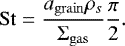
The dynamics of dust grains are strongly dependent on the grain size. A grain with a large surface area relative to its mass is well coupled to the gas and will not act significantly different from a molecule in the gas. Solid bodies with a very small surface area relative to its mass, for example, planetesimals, will not be influenced by the gas pressure or turbulence, their motions are then completely governed by gravitational interactions. Dust particles with sizes between these extremes will be influenced by the presence of the gas in various ways. To quantify these regimes it is useful to consider a quantity known as the Stokes number: The Stokes number is, assuming Epstein drag and spherical particles in a vertically hydrostatic disk, given by (Weidenschilling 1977; Birnstiel et al. 2010):
 (6)
(6)
Particles with a very small Stokes number ( ≪1) are very well coupled to the gas and the gas pressure gradients and particles with very large Stokes number ( ≫1) are decoupled from the gas.
The coupling between gas and dust determines both the diffusivity of the dust, that is, how well the dust mixed due to turbulent motions of the disk as well as advection of the dust due to bulk flows of the gas. Youdin & Lithwick (2007) derived that the diffusivity Ddust of a particle with a certain Stokes number can be related to the gas diffusivity by:
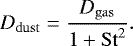 (7)
(7)
Similarly the advection speed of dust due to gas advection can be given by:
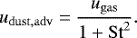 (8)
(8)
When particles are not completely coupled to the gas they are also no longer completely supported by the gas pressure gradient. The gas pressure gradient, from high temperature, high density material close to the star, to low temperature, low density material far away from the star provides an outwards force, such that the velocity with which the gas has a stable orbit around the star is lower than the Keplerian velocity. Particles that start to decouple from the gas thus also need to speed up relative to the gas to stay in a circular orbit. This induces a velocity difference between the gas and the dust particles. The velocity difference between the gas velocity and a Keplerian orbital velocity is given by:
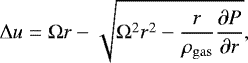 (9)
(9)
with P the pressure of the gas. We note that in the case of a positive pressure gradient, the gas will be moving faster than the Keplerian velocity
As a result of this velocity difference the particles are subjected to a drag force, which, in the case of a negative pressure gradient, removes angular momentum from the particles. The loss of angular momentum results in an inwards spiral of the dust particles. This process is known as radial drift. The maximal drift velocity can be given as (Weidenschilling 1977):
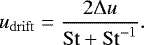 (10)
(10)
The drift velocity will thus be maximal for particles with a Stokes number of unity. Drift velocities of ~1% of the orbital velocity are typical for particles with a Stokes number of unity.
The dynamics of dust are thus intrinsically linked to the size, or rather size distribution of the dust particles. The dust size distribution is set by the competition of coagulation and fragmentation2. When two particles collide in the gas they can either coagulate, that is, the particles stick together and continue on as a single larger particle, or they can fragment, the particles break apart into many smaller particles. The outcome of the collision depends on the relative velocity of the particles and their composition. At low velocities particles are expected to stick, while at high velocities collisions lead to fragmentation. The velocity that sets the boundary between the two outcomes is called the fragmentation velocity. For pure silicate aggregates the fragmentation velocities are low (1 m s−1 ) while aggregates with a coating of water ice can remain intact in collisions with relative velocities up to a order of magnitude higher (Blum & Wurm 2008; Gundlach & Blum 2015).
Dust size distributions resulting from the coagulation and fragmentation processes can generally not be computed analytically. Calculations have been done for both static and dynamic disks (Brauer et al. 2008; Birnstiel et al. 2010; Krijt & Ciesla 2016). These models are very numerically intensive and do not lend themselves to the inclusion of additional physics and chemistry nor to large parameter studies. As such we will use the simplified dust evolution prescription from Birnstiel et al. (2012). This prescription has been benchmarked against models with a more complete grain growth and dust dynamics prescription from Brauer et al. (2008). The prescription only tracks the ends of the dust size distribution, the smallest grains of set size and the largest grains at a location in the disk of a variable size. As this prescription is a key part of the model we will reiterate some of the key arguments, equations and assumption of this prescription here, for a more complete explanation, see Birnstiel et al. (2012).
The prescription assumes that the dust size distribution can be in one of three stages at any point in the disk. Either the largest particles are still growing, the largest particle size is limited by radial drift, or the largest particle size is limited by fragmentation. In the first and second case, the size distribution is strongly biased towards larger sizes. In the final case the size distribution is a bit flatter (see, Brauer et al. 2008). The size distribution in all cases is parametrised by a minimal grain size, the monomer size, a maximal grain size, which depends on the local conditions, and the fraction of mass in the large grains.
From physical considerations one can write a maximal expected size of the particles due to different processes. Growth by coagulation is limited by the amount of collisions and thus by the amount of time that has passed. The largest grain expected in a size distribution at a given time is given by:
![Mathematical equation: $ a_{\mathrm{grow}}(t) = a_{\mathrm{mono}}\exp\left[{\frac{t-t_0}{\tau_{\mathrm{grow}}}}\right], $](/articles/aa/full_html/2018/03/aa32056-17/aa32056-17-eq13.png) (11)
(11)
where amono is the monomer size, t0 is the starting time, t is the current time and τgrow is the local growth time scale, given by:
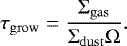 (12)
(12)
Radial drift moves the particles inwards: the larger the particles, the faster the drift. There is thus a size at which particles are removed faster due to radial drift than they are replenished by grain growth, limiting the maximal size of particles. This maximal size is given by:
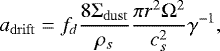 (13)
(13)
with fd a numerical factor, ρs is the density of the grainsand γ is the absolute power law slope of the gas pressure:
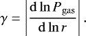 (14)
(14)
As mentioned before, particles that collide with high velocities are expected to fragment. For this model we consider two sources of relative velocities. One source of fragmentation is differential velocities due to turbulence (see, Ormel & Cuzzi 2007, for a more complete explanation). This limiting size is given by:
 (15)
(15)
where ff is a numerical fine tuning parameter and uf is the fragmentation velocity. The other source of fragmentation considered is different velocities due to different radial drift speeds. The limiting size for this process is given by:
 (16)
(16)
N is the average Stokes number fraction between two colliding grains, here we use N = 0.5.
The size distribution at a location in the disk spans from the monomer size (amono) to the smallest of the four limiting sizes above. In the model the grains size distribution is split into “small” and “large” grains. The mass fraction of the large grains depends on the process limiting the size: if the grain size is limited by fragmentation ( min (afrag, adf) < adrift), the fraction of mass in large grains (fm, frag) is assumed to be 75%. If the grain size is limited by radial drift (adrift < min(afrag, adf)), the fraction of mass in large grains (fm, drift) is assumed to be 97%. These fractions were determined by Birnstiel et al. (2012) by matching the simplified model to more complete grain-growth models.
Using these considerations the advection-diffusion equation for the dynamics of the dust can be rewritten:
![Mathematical equation: \begin{align} \frac{\partial {\UpSigma}_{\mathrm{dust}}}{\partial t} &=& \frac{1}{r}\frac{\partial}{\partial r} \left[\vphantom{\frac12}\left( u_{\mathrm{dust,\,s\,}} r (1-f_m){\UpSigma}_{\mathrm{dust}} + u_{\mathrm{dust,\,l\,}} r f_m{\UpSigma}_{\mathrm{dust}}\right) \right. \\ && +r {\UpSigma}_{\mathrm{gas}} \left( D_{\mathrm{dust,\,s\,}} \frac{\partial}{\partial r}\left(\frac{(1-f_m){\UpSigma}_{\mathrm{dust}}}{{\UpSigma}_{\mathrm{gas}} }\right) \right. \\ && + \left.\left. D_{\mathrm{dust,\,l\,}} \frac{\partial}{\partial r}\left(\frac{f_m{\UpSigma}_{\mathrm{dust}}}{{\UpSigma}_{\mathrm{gas}} }\right) \right) \right], \end{align}](/articles/aa/full_html/2018/03/aa32056-17/aa32056-17-eq19.png) (17)
(17)
where  ,
,  where udrift is the velocity due to radial drift (Eq. (10)). Here it is assumed that the large grains never get a Stokes number larger than unity, which holds for the models presented here.
The final part of the dynamics concerns the ice on the dust. The ice moves with the dust, so both the large scale movements as well as the mixing diffusion of dust must be taken into account. For the model we assume that the ice is distributed over the grains according to the mass of the grains. This means that if large grains have a mass fraction fm , then the large grains will have the same mass fraction of fm of the available ice. This is a reasonable assumption, as long as the grain size distribution is in fragmentation equilibrium and the largest grains are transported on a timescale longer than the local growth timescale. The algorithm used here forces the latter condition to be true everywhere in the disk, while the former condition is generally true for the CO2 and H2 O icelines (Brauer et al. 2008), but not for the CO iceline (Stammler et al. 2017). With this assumption the advection-diffusion equation forthe ice can be written as:
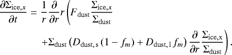 (18)
(18)
Here Fdust is the radial flux of dust, this is given by:
 (19)
(19)
2.3 Model parameters
For our study, we pick a disk structure that should be representative of a young disk around a one solar mass star. The initial surface density structure is given by:
![Mathematical equation: $ {\UpSigma}_{\mathrm{gas}}(r) = {\UpSigma}_{1\,\mathrm{AU}} \left(\frac{r}{1\,\mathrm{AU}}\right)^{-p} \exp\left[\left(-\frac{r}{r_{\mathrm{taper}}}\right)^{2-p}\right], $](/articles/aa/full_html/2018/03/aa32056-17/aa32056-17-eq24.png) (20)
(20)
where p controls the steepness of the surface density profile, rtaper the extent ofthe disk and Σ1 AU sets the normalisation of the surface density profile. For our models we use p = 1 and rtaper = 40 AU. The temperature profile is given by a simple power law:
 (21)
(21)
The disk is assumed to be viscous with a constant α, as such there is a constraint on the power law slopes p and q, if we want the gas surface density to be a self similar solution to Eq. (1), it is required to have p + q = 3∕2 (Hartmann et al. 1998).
To calculate the volume densities, a vertical Gaussian distribution of gas with a scale height Hp (r) = hpr, with hp = 0.05, is used.
The disk is populated with particles of 0.1 μm at the start of the model, this is also the size of the small dust in the model. The gas-to-dust ratio is taken to be 100 over the entire disk. The density of the grains is assumed to be 2.5 g cm−3 and grains are assumed to be solid spheres.
The molecules are initially distributed through simple step functions. These step functions have a characteristic radius “iceline” which differentiates between the inner disk and the outer disk. Within this radius the gas phase abundance of the molecule is initialised, outside of this radius the solid phase abundance is initialised. Water is distributed equally through the disk with an abundance of 1.2 × 10⁻⁴, whereas CO2 is initially depleted in the inner disk with an abundance of 10−8 (Pontoppidan et al. 2011; Bosman et al. 2017) and has a high abundance in the outer disk of 4 × 10⁻⁵. This ice abundance of CO2 is motivatedby the ISM ice abundance (Pontoppidan et al. 2008; Boogert et al. 2015), cometary abundances (Le Roy et al. 2015)and chemical models of disk formation (Drozdovskaya et al. 2016).
A summary of the initial conditions, fixed and variable parameters is given in Table 1.
Initial conditions, fixed parameters and variables.
2.4 Boundary conditions
Due to finite computational capabilities, the calculation domain of the model needs to be limited. The assumptionsmade for the edges can have significant influences on the model results. For the inner edge, it is assumed that gas leaves the disk with an accretion rate as assumed from a self similar solution (p + q = 3∕2) according tothe viscosity and surface density at the inner edge. The accretion rate is given by:
 (22)
(22)
All gas constituents advect with the gas over the inner boundary or, in the case of large grains, drift over the boundary. Diffusion over the inner boundary is not possible. For the outer boundary, the assumption is made that the surface density of gas outside the domain is zero. Again viscous evolution or an advection process can remove grains and other gas constituents from the computational domain.
3 Chemical processes
3.1 Freeze-out and sublimation
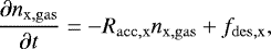
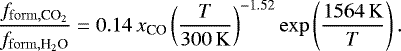
Freeze-out and sublimation determine the fraction of a molecule that is in the gas phase and the fraction that is locked up on the grains. Freeze-out of a molecule, or a molecule’s accretion onto a grain is given by the collision rate of a molecule with the grain surface times the sticking fraction, fs, which is assumed to be unity:
 (23)
(23)
where σdust is the average dust surface area, ngrain is the number density of grains and the thermal velocity  , with k the Boltzmann constant, T the temperature and mx the mass of the molecule. Molecules that are frozen-out on the grain can sublimate or desorb. For a grain covered with many monolayers of ice, the rate per unit volume for this process is given by:
![Mathematical equation: $ f_{\mathrm{des,x}} = R_{\mathrm{des,x}} n_{\mathrm{x,ice}} = p_x \sigma_{\mathrm{dust}} n_{\mathrm{grain}} N_{\mathrm{act}} \exp\left[-\frac{E_{\mathrm{bind}}}{kT}\right], $](/articles/aa/full_html/2018/03/aa32056-17/aa32056-17-eq29.png) (24)
(24)
where px is the zeroth-order “prefactor” encoding the frequency of desorption attempts per unit surface area, σdust is the surface area per grain, ngrain is the number density of grains. Nact is the number of active layers, that is, the number of layers that can participate in the sublimation, Nact = 2 is used, T is the dust temperature, which we take equal to the gas temperature. For mixed ices this rate can be modified by a covering fraction χx = nice, x∕∑ xnice, x, however, this is neglected here. We note that fdes,x in its current form is independent of the amount of molecules frozen out on the dust grains. Using these rates we get the following differential equation:
 (25)
(25)
which has an analytical solution:
![Mathematical equation: \begin{align} n_{\mathrm{x,gas}}(t) &=& \min\left[\vphantom{\frac12}n_{\mathrm{x,tot}},\left(n_{\mathrm{x,gas}}(t_0) - \frac{f_{\mathrm{des,x}}}{R_{\mathrm{acc,x}}}\right)\right. \\ && \times \left. \exp\left(-R_{\mathrm{acc,x}}(t-t_0)\right) + \frac{f_{\mathrm{des,x}}}{R_{\mathrm{acc,x}}}\right]. \end{align}](/articles/aa/full_html/2018/03/aa32056-17/aa32056-17-eq31.png) (26)
(26)
where nx,tot is the total number density of a molecule (gas and ice). The number density of ice is given by:
 (27)
(27)
The ice line temperature, defined as the temperature for which nx,gas = nx,dust, that is, when freeze-out and sublimation balance, depends on the total number density of the molecule considered. At lower total molecule number densities, the iceline will be at lower temperatures.
For CO2 we use a binding energy of 2900 K, representative for CO2 mixed with water (Sandford & Allamandola 1990; Collings et al. 2004). More recent measurements have suggested that the binding energy is lower, around 2300 K (Noble et al. 2012). Using the lower binding energy moves the CO2 iceline further out from 90 to 80 K or from 6 to 8 AU in our standard model. The prefactor,  , of 9.3 × 1026 cm−2 s−1 from (Noble et al. 2012) is used. The change in iceline location has a minimal effect on the evolution of the abundance profiles. The mixing time-scale becomes longer at larger radii which would increase mixing times. For H2 O a binding energy of 5600 K and prefactor,
  , of 1030 cm−2 s−1 (Fraser et al. 2001).
3.2 Midplane formation and destruction processes
Radial drift and radial diffusion and advection will quickly move part of the outer disk CO2 ice reservoir into the inner disk, enhancing the inner disk abundances. To get a good measure of the amount of CO2 in the innerdisk it is necessary to also take into account the processes that form and destroy CO2 in gas and ice. The density is highest near the mid-plane, as such this is where formation and destruction process are expected to be most relevant for the bulk of the CO2. However, in the less dense upper layers, there are UV-photons that can dissociate and ionise molecules, possibly influencing the overall abundance of CO2.
3.2.1 Gas-phase formation of CO2
The formation of CO2 in the inner disk mainly goes through the warm gas-phase route. Here CO2 forms through the reaction CO + OH →CO2 + H. The reaction has a slight activation barrier of 176 K (Smith et al. 2004). The parent molecule CO is very stable and is expected to be present at high abundances in the inner disk (10−4) (Walsh et al. 2015). The OH radical is expected to be less abundant, and it is the fate of this radical that determines the total production rate of CO2 . OH is formed either directly from H2O photodissociation (Heays et al. 2017), or by hydrogenation of atomic oxygen, O +H2 →OH + H, in a reaction that has an activation barrier of 3150 K (Baulch et al. 1992). The atomic oxygen itself also has to be liberated from, in this case, either CO, CO2 or H2 O by X-rays or UV-photons. The production rate of CO2 is thus severely limited if there is no strong radiation field present to release oxygen from one of the major carriers.
The CO2 formation reaction, CO + OH →CO2 + H, has competition from the H2O formation reaction, OH + H2 →H2O + H. The hydrogenation of OH has a higher activation energy, 1740 K, than the formation of CO2 , but since H2 is orders of magnitude more abundant than CO, the formation of water will dominate over the formation of CO2 at high temperatures. The rate for CO2 formation is given by (Smith et al. 2004):
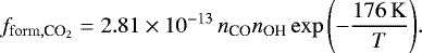 (28)
(28)
The formation rate for H2O formation is given by (Baulch et al. 1992):
 (29)
(29)
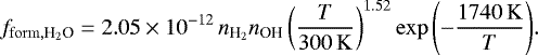
This means that the expected  fraction from formation is:
 (30)
(30)
This function is plotted in Fig. 1 which shows that the formation of CO2 is faster below temperatures of 150 K, whereas above this temperature formation of water is faster. Above a temperature of 300 K water formation is a thousand times faster than CO2 formation. The implication is that gaseous CO2 formation is only effective in a narrow temperature range, 50–150 K, and then only if OH is present as well, requiring UV photons or X-rays to liberate O and OH from CO or H2O.
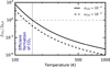 |
Fig. 1 Ratio of the CO2 to H2 O formation rate from a reaction of OH with CO and H2 respectively. Hydrogenation of OH to H2O dominates above 150 K. Formation times of CO2 and H2 O from OH are faster than the inner disk mixing time for all temperatures considered here. |
3.2.2 Destruction of CO2: cosmic rays
Cosmic rays, 10–100 MeV protons and ions, have enough energy to penetrate deeply into the disk. Cosmic-rays can ionise H2 in regions where UV photons and X-rays cannot penetrate. The primary ionisation as well as the collisions of the resulting energetic electron with further H2 creates electronically excited H2 as well as excited H atoms. These excited atoms and molecules radiatively decay, resulting in the emission of UV-photons (Prasad & Tarafdar 1983). These locally generated UV-photons can dissociate and ionise molecules. Here only the dissociation rate of CO2 is taken into account as ionisationof CO2 by this process is negligible. Following Heays et al. (2017) the destruction rate of species X is written as:
 (31)
(31)
where  is the direct cosmic ray ionisation rate of H2, xX is the abundance of species X w.r.t. H2 , P(λ) is the photon emission probability per unit spectral density for which we use the spectrum from Gredel et al. (1987). pX (λ) is the absorption probability of species X for a photon of wavelength λ. This probability is given by:
 (32)
(32)
where  is the wavelength dependent destruction or absorption cross section of species X and
  is the dust cross section per hydrogen molecule. For the calculation of the cosmic-ray dissociation rate of CO2 we assume that the destruction cross section in the UV is equal to the absorption cross section for CO2 , that is, every absorption of a photon with a wavelength shorter than 227 nm leads to the destruction of a CO2 molecule. For the calculations the cross sections from Heays et al. (2017) are used3 . These cross sections can also be used to compute destruction rates for CO2 by stellar UV radiation in the surface layers of the disk.
The dust absorption is an important factor in these calculations and can be the dominant contribution to the total absorption in parts of the spectrum. The dust absorption greatly depends on the dust opacities assumed. A standard ISM dust composition was taken following Weingartner & Draine (2001), the mass extinction coefficients are calculated using Mie theory with the MIEX code (Wolf & Voshchinnikov 2004) and optical constants by Draine (2003) for graphite and Weingartner & Draine (2001) for silicates. Grain sizes are distributed assuming an MRN distribution starting at 5 nm, with varying maximum size are used. The resulting mass opacities and cross sections are shown in Fig. A.1.
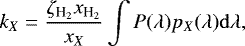
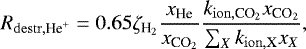
Cosmic ray induced destruction rates for CO2 are calculated for each dust size distribution for a range of CO2 abundances between 10−8 and 10−4. The o-p ratio of H2, important for the H2 emission spectrum, is assumed to be 3:1, representative for high temperature gas. The abundances of the other shielding species used in the calculation are shown in Table 2. The destruction rate for CO2 is plotted in Fig. 2.
The CO2 destruction is faster for grown grains and low abundances of CO2. At abundances above 10−7, the strongest transitions start to saturate, lowering the destruction rate with increasing abundance. Even though the dust opacity changes by more than an order of magnitude, the dissociation rates stay within a factor of 3 for all CO2 abundances. This is due to the inclusion of H2O into our calculations. H2 O has large absorption cross sections in the same wavelength regimes as CO2. When H2 O is depleted, such as would be expected between the H2O and CO2 icelines, CO2 destruction rates increase, especially for the largest grains. Even in this optimal case, the destruction rate for CO2 is limited to 2 × 10⁻¹³ s−1 for typical  of 10−17 s−1.
Aside from generating a UV field, cosmic-rays also create ions, the most important of these being He+ . Due to the large ionisation potential of He, electron transfer reactions with He+ generally lead to dissociation of the newly created ion. For example, CO2 + He+ preferably leads to the creation of O + CO+. Destruction of CO2 due to He+ is limited by the creation of He+ and the competition between CO2 and other reaction partners of He+. The total reaction rate coefficient of CO2 with He+ is 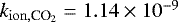 cm3 s−1 (Adams & Smith 1976). The three main competitors for reactions with He+ are H2 O, CO and N2 , with reaction rate coefficients of
  , kion , CO = 1.6 × 10⁻⁹ and
  cm3 s−1 respectively (Mauclaire et al. 1978; Anicich et al. 1977; Adams & Smith 1976). Assuming a cosmic He+ ionisation rate of
  (Umebayashi & Nakano 2009), the destruction rate for CO2 due to He+ reaction can be written as,
 (33)
(33)
where the sum is over all reactive collision partners of He+ of which CO, N2 and H2 O are most important. For typical abundances of He of 0.1 and N2, CO and H2O of 10−4,  is below
  for all CO2 abundances.Thus cosmic-ray induced photodissociation will always be more effective than destruction due to He+ .
Altogether the destruction time-scale for midplane CO2 by cosmic ray induced processes is long, ~3 Myr for a  s−1. The latter value is likely an upper limit for the inner disk given the possibility of attenuation and exclusion of cosmic rays (Umebayashi & Nakano 1981; Cleeves et al. 2015).
Gas-phase abundances assumed for the cosmic ray induced dissociation rate calculations.
 |
Fig. 2 Dissociation rate of CO2
due to cosmic ray induced photons, for different dust size distributions. Solid lines are for condition inside of the
H2 O
iceline, dashed lines for conditions outside of the H2O
iceline. The efficiency multiplied by |

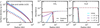 |
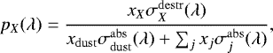
Fig. 3 Time evolution series for a model without grain growth. This model assumes an α of 10−3 . Left: surface density of the gas (solid lines) and solids (dashed lines), the solid surface density is the sum of the dust and ice surface densities, it has been multiplied by a factor of 10 for visualization. Middle: abundance of CO2 . Right: abundance of H2O. |
3.2.3 Destruction of CO2: gas-phase reactions
In warm gas it is possible to destroy CO2 by endothermic reactions with H or H2 (Talbi & Herbst 2002). The reaction
 (34)
(34)
has an activation barrier of 13 300 K and a pre-exponential factor of 2.5 × 10⁻¹⁰ cm3 s−1 for temperatures between 300 and 2500 K (Tsang & Hampson 1986) while the reaction
 (35)
(35)
has an activation barrier of 56 900 K and has a pre-exponential factor of 3.3 × 10⁻¹⁰ cm3 s−1 at 1000 K. This means that for gas at 300 K, an H2 density of 1012 cm−3, and a corresponding H density of 1 cm−3, the rate for destruction by atomic hydrogen is 1.4 × 10⁻²⁹ s−1, while the destruction rate by molecular hydrogen is 1.4 × 10−80 s−1. Both are far too low to be significant in the inner disk. However, if the atomic H abundance is higher, destruction of CO2 by H can become efficient at high temperatures. As such the destruction of CO2 becomes very dependent on the formation speed of H2 at high densities and temperatures. The CO2 abundance as a function of temperature for a gas-phase model is shown in Fig. B.1. Temperatures of >700 K are needed to lower the CO2 abundance below 10−7, even with a high atomic H abundance.
3.3 Simulating spectra
To compare the model abundances with observations, infrared spectra are simulated with the thermochemical code DALI (Bruderer et al. 2012; Bruderer 2013). DALI is used to calculate a radial temperature profile, from dust and gas surface density profiles and stellar parameters. The viscous evolution model is initialised using the same surface density distribution as the DALI model. The temperature slope q is taken so that the surface density slope p is consistent with a self-similar solution q = 1.5 − p = 0.9. The temperature at 1 AU is taken from the midplane temperatures as calculated by the DALI continuum ray-tracing module. No explicit chemistry is included in this version of DALI, but the abundances are parametrised using the output of the dynamical model. The viscous model run with α = 10−3, uf = 3 m s−1 and a CO2 destruction rate varying between 10−13 and 10−9 s−1. The results from Sect. 4.4 show that these parameters represent the bulk of the model results.
After simulating 1 Myr of evolution, the gas-phase CO2 abundance profile is extracted as function of temperature and interpolated onto the DALI midplane temperatures. The abundance is taken to be vertically constant up to the point where AV = 1. In some variations an abundance floor of 10−9 or 10−8 is used for cells with AV > 1 to simulate local CO2 production. Using the resulting abundance structure, the non-LTE excitation of CO2 is calculated using the rate coefficients from Bosman et al. (2017). Finally the DALI line ray-tracing module calculates the line fluxes for CO2 and its 13C isotope.
For calculating the spectra, the same disk model is used as in Bruderer et al. (2015) and Bosman et al. (2017). The model is based on the disk AS 205 N. The parameters for the DALI models can be found in Table 3. For more specifics on the modelling of the spectra and adopted parameters, see Bruderer et al. (2015) and Bosman et al. (2017). To simulate the high gas-to-dust ratios that are inferred from water observations (Meijerink et al. 2009), the overall gas-to-dust ratio is set at 1000 throughout the disk. The artificially high gas-to-dust ratio does not affect any of the modelling, except for the line formation, which is only sensitive to the upper optically thin layers of the disk. High gas-to-dust ratios effectively mimic settled dust near the midplane containing ~90% of the dust mass.
Adopted standard model parameters for the DALI modelling.
4 Results
4.1 Pure viscous evolution
To start, a dynamical model without grain growth and without any chemistry (except for freeze-out and desorption) is investigated. Figure 3 shows the time evolution for a model with α =10−3. As expected, the total gas and dust surface densities barely change over 106 yr. The gas anddust evolve viscously, some mass is accreted onto the star while the outer disk spreads a little bit. There are no changes in gas-to-dust ratio in the disk.
The water abundance in the right panel of Fig. 3 shows no evolution at all. This is to be expected because the only radial evolution is due to the gas viscosity, which affects gas and dust equally. Diffusion of the icy dust grains is equally quick as the diffusion of the water vapour. This means that all the water vapour that diffuses outwards is compensated by icy dust grains diffusing inwards.
The abundance of CO2 in the middle panel of Fig. 3 does show evolution. Initially there is only a little bit of CO2 gas in the inner disk, but a large amount of ice in the outer disk. The abundance gradient together with the viscous accretion makes the icy CO2 move inwards, filling up the inner disk with CO2 gas. This continues for about 1 × 10⁶ yr until the gaseous abundance of CO2 is equal to the abundance of icy CO2. This time-scale directly scales with the assumed α parameter. For α = 10−4 it takes more than 3 Myr to get a flat abundance profile in the inner disk.
4.2 Viscous evolution and grain growth
For the models including grain growth, we tested a range of fragmentation velocities from 1 to 30 m s−1 . For some ofthese models, especially those with low fragmentation velocities and high α, the results are indistinguishable from the case without grain growth. Figures 4 and 5 show two models where the effect of grain growth and resulting drift can be seen.
Figure 4 shows the surface density and abundance evolution for a model with a fragmentation velocity of 3 m s−1 as appropriate for pure silicate grains. The surface density of the dust shows a small evolution due to radial drift. Instead of decreasing, the surface density of dust in the inner 4 AU slightly increases in the first 300 000 yr due to the supply of dust particles from outside this radius.
The abundance profiles in Fig. 4 show distinct effects of radial drift. Both the gaseous H2 O and CO2 abundances are high at all times due to the influx of drifting icy grains. There is also a decrease in the abundance of ices at large radii. This is because the grains carrying the ices have moved inwards, increasing the gas-to-ice ratios.
The models are not in steady state after 1 Myr. If these models are evolved further, at first the abundances of H2 O and CO2 will increasefurther. At some point in time the influx of dust will slow down, because a significant part of the dust in the outer disk will have drifted across the snowline. At this point the inner disk abundances of H2 O and CO2 start to decrease as these molecules are lost due to accretion onto the star but no longer replenished by dust from the outer disk. For the model shown in Fig. 4 the average gas-to-dust ratio in the disk would be around 500 after 3 Myr.
For higher α the effects of radial drift are limited as the high rate of mixing smooths out concentration gradients created by radial drift. At the same time the maximum grain size is limited due to larger velocity collisions at higher turbulence. As such, for α = 0.01 a fragmentation velocity higher than 10 m s−1 is needed to see significant effects of radial drift and grain growth.
For lower α the effects of grain growth get more pronounced, 90% of the dust mass is accreted onto the star in 2.5 Myr for a fragmentation velocity of 1 m s−1. In this time a lot of molecular material is released into the inner disk and peak abundances of 10−3 and 10−2 are reached for CO2 and H2 O, respectively, after 1 Myr of evolution. Due to the low turbulence in the gas, the volatiles released are not well mixed, neither inwards nor outwards, so there is no strong enhancement of the ice surface density just outside of the iceline. An overview of the different model evolutions can be found in Appendix C.
Increasing the fragmentation velocity allows grains in the model to grow to larger sizes, leading again to larger amounts of radial drift. Figure 5 shows the evolution of the same model as shown in Fig. 4, but with a fragmentation velocity of 30 m s−1 , representative for grains coated in water ice. The solid surface density distribution clearly shows the effects of grain growth. At all radii, mass is moved inwards at a high rate. When the silicate surface density has dropped by an order of magnitude, a local enhancement in the surface density of the total solids is seen at the icelines. This enhancement is about a factor of 2 for both icelines.
The gas-phase abundances of CO2 and H2 O both show a large increase in the first 3 × 10⁵ yr due to the large influx of icy pebbles. At later times, the abundances are decreased again as the volatiles are accreted onto the star. After 3 × 10⁶ yr the H2 O and CO2 abundances are lower than 10−5.
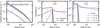 |
Fig. 4 Time evolution series for a model with grain growth. This model assumes an α of 10−3 . The fragmentation velocity for this model is 3 m s−1. Panels as in Fig. 3. |
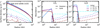 |
Fig. 5 Time evolution series for a model with grain growth. The fragmentation velocity for this model is 30 m s−1 and α = 10−3. The verticalscales are different from Figs. 3 and 4. Panels as in Fig. 3. |
4.3 Viscous evolution and CO2 destruction
The models shown in Figs. 3–5 without any chemical processing predict CO2 abundances that are very high in the inner regions, 10−5–10−4, orders of magnitude higher that the value of ~10−8 inferred from observations (Pontoppidan & Blevins 2014; Bosman et al. 2017). There are multiple explanations for this disparity, both physical and chemical, which are discussed in Sect. 5. Here we investigate how large any missing chemical destruction route for gaseous CO2 would need to be. As discussed in Sect. 3 and Appendix sectionlinking B.1 , midplane CO2 can only be destroyed by cosmic-ray induced processes in the current networks. However, both cosmic ray induced photodissociation and He+ production are an order of magnitude slower than the viscous mixing time. We therefore introduce additional destruction of gaseous CO2 with a rate that is a constant over the entire disk. This rate is varied between 10−13 and 10−9 s−1 to obtain agreement with observations. For comparison, the cosmic ray induced process generally have a rate of the order of 10−14 s−1 (see Sect. 3.2.2). The rate is implemented as an effective destruction rate, so there is no route back to CO2 after destruction. To get the absolute rate one has to also take into account the reformation efficiency, but that can be strongly dependent on the destruction pathway, of which we are agnostic. These efficiencies are discussed in Sect. 5 and Appendix B.
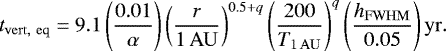
Figure 6 shows the abundance evolution for a model where only gaseous CO2 is destroyed, at a rate of 10−11 s−1. In this case the innermost parts of the disk are empty of CO2, whereas the abundance of CO2 reaches values close to the initial ice abundances around the iceline. Due to the constant destruction of CO2 near the iceline, the actual ice abundance of CO2 is also lower than the initial value.
The left panel of Fig. 7 shows the CO2 abundance distribution for models with α = 10−3. The abundance profiles after 1 Myr of evolution are presented, when a semi-steady state has been reached. The peak abundance and peak width of the CO2 gas abundance profile both depend on the assumed destruction rate: a higher rate leads to a lower peak abundance and a narrower peak, while a lower rate leads to the opposite. A rate of ~ 10−11 s−1 or higher is needed to decrease the average gaseous CO2 abundance below the observational limit (see below). Increasing the rate moves the location of the iceline further out, as the total available CO2 near the iceline decreases. The viscosity also influences the width of the abundance profile, higher viscosities lead to a broader abundance peak.
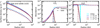 |
Fig. 6 Timeevolution series for a model without grain growth but with a constant destruction rate of gaseous CO2 of 10−11 s−1. This model assumes an α of 10−3 . Panels as in Fig. 3, but with different vertical scales. |
 |
Fig. 7 Abundance of CO2 as function of radii for models with different destruction rates of CO2. These modeluse α = 10−3 and uf = 0 m s−1 (left) and uf = 3 m s−1 (right). Abundance profiles after 1 Myr of evolution are shown. At this point the disk has reached a semi steady state. A destruction rate of at least 10−11 s−1 is needed to keep the averaged CO2 abundance below the observational limit. The iceline is further out for models with higher destruction rates as the destruction of gas-phase CO2 lowers the total abundance of CO2 within 10 AU where CO2 can sublimate. |
4.4 Viscous evolution, grain growth and CO2 destruction
The next step is to include CO2 destruction in viscous evolution models with grain growth. Here only models that retain the disk dust mass, that is, models that have an overall gas-to-dust ratio smaller than 1000 after 1 Myr of evolution are considered since there is no observational evidence for very high gas-to-dust ratios. This means that the grains in our models do not reach pebble sizes such as have been inferred from observations (e.g. Pérez et al. 2012; Tazzari et al. 2016). It is unclear how these large grains are retainedin the disk as the radial drift timescale for these particles is expected to be shorter than the disk lifetime (e.g. Birnstiel et al. 2010; Krijt et al. 2016). The requirement of dust retention restricts our models to α =10−4 and uf = 1 m s−1, α =10−3 and uf = 1, 3 m s−1, and α = 10−2 and uf = 1, 3, 10 m s−1.
The abundance profiles for different CO2 destruction rates are shown in the right panel of Fig. 7 for the model with α = 10−3 and uf = 3 m s−1. The abundance profiles are determined after 1 Myr, when the disk is in a semi-steady state. A destruction rate higher than 10−12 s−1 will create an abundance profile with clear abundance maximum at the iceline, but for this rate 10−12 s−1 the disk surface area averaged CO2 abundance is still higher than the observed value for both cases. Only for a rate of around 10−10 s−1 do the models predict an abundance profile with a disk surface area averaged CO2 abundance that is consistent with the high end of the observations. Only the models with destruction rate higher than 10−9 s−1 have a peak in the abundance that is consistent with the maximal inferred abundances from the observations. As shown in Fig. 7 the model with a rate of 10−11 s−1 will create a spectrum consistent with the observations, even though the average CO2 abundance is higher than the observed abundance limit.
For the selected models, the effect of different fragmentation velocities is small, with differences in peak abundances less than a factor of five between similar models, as seen in Fig. 7. This is unsurprising as the selection criteria for the models only consider models that have a transport velocity of solids that is less than an order of magnitude faster than the transport velocity of the model without grain growth and radial drift. For models with faster growth it becomes more arbitrary to give a representative abundance profile as semi steady state is not reached at any point in time before the disk is depleted of most of the dust and volatiles in the inner regions. However, for very young disks that may have very efficient radial drift of grains, a high gas-phase CO2 abundance is expected within the CO2 iceline unless the destruction rate is 10−11 s−1 or higher.
4.5 Model spectra
The spectralmodelling the focuses on the CO2 bending mode around centred at 15 μm. This bending mode has a strong Q-branch that has been observed by Spitzer in protoplanetary disks (Carr & Najita 2008; Pontoppidan et al. 2010). This region also has a weaker feature due to the Q-branch of 13CO2 at 15.42 μm which can be used, together with the 12CO2 Q-branch, to infer information on the abundance structure (Bosman et al. 2017).
For the model with α = 10−3 and  , the 2D abundance distribution assumed for the ray-tracing is shown in Fig. 8. The enhanced CO2 abundance around the iceline shows up clearly. The results of the continuum ray-tracing can be found in Fig. 5 of Bosman et al. (2017). The temperature at 1 AU is 320 K. This is higher than the value assumed for the models in the previous sections and is in line with the high luminosity of the modelled source of 7.7 L⊙. The higher temperaturemoves the CO2 iceline slightly further out. The abundance profiles from the viscous model with dust growth and CO2 destruction are still very similar to those from the previous section.
Figure 8 also shows the emitting region of the CO2 Q(6) line for both isotopologues. This is one of the strongest lines in the CO2 spectrum and part of the Q-branch. As such it is a good representative for the complete Q-branch. Due to its high abundance, the 12CO2 lines have a high optical depth over a larger area in the disk. As such a large part of the disk contributes to the emission of the 12 CO2 lines. For 13 CO2 the emission is from a more compact area, close to the peak in CO2 abundance.
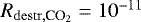
Figure 9 shows CO2 spectra for different destruction rates and abundance floor of 10−8. Line-to-continuum ratios for the individual R and P branch linesare all greater than 0.01 and are detectable by JWST (Bosman et al. 2017). Note that only even J levels exist in the vibrational ground state, so P, Q and R branch lines exist only every other J for this band. Both the 12CO2 and the 13CO2 Q-branch fluxes are influenced by the different destruction rates. For a rate of 10−12 s−1 the 12CO2 Q-branch is a factor of two brighter than for the higher rates, which give fluxes very similar in magnitude for the 12 CO2 Q-branch. For 13 CO2 the model with a destruction rate of 10−12 s−1 is a least a factor of five brighter than the models with higher rates of 10−11 s−1 and 10−10 s−1. Since the latter two 12CO2 spectra are indistinguishable observationally, a conservative lower limit to the destruction rate of 10−11 s−1 is chosen. For 13CO2 however, there is a factor of three difference between the two higher rate models; here the 13 CO2 Q-branch flux is determined by subtracting the contribution from the 12CO2 P(23)-line assuming it is the same as that of the neighbouring P(21) line.
The fluxratio of the 13CO2 Q-branch over the 12CO2 Q-branch is shown in Fig. 10 for a range of CO2 destruction rates. Three regimes can be seen. For ratios larger than ~0.13 the CO2 released from the ice dominates the abundance profile and spectrum, due to the relatively low destruction rate. The high CO2 column, dueto the high abundance around the iceline sets the small flux ratio. At ratios smaller than 0.03, corresponding to destruction rates larger than 5 × 10⁻¹¹ s−1, the CO2 released from the ice at the iceline is destroyed so fast that it cannot leave an imprint on the Q-branch fluxes. In the region in between, both the CO2 released at the iceline as well as the upper layer CO2 influence the spectra, as such the flux ratio not only depends on the CO2 destruction rate, but also on the CO2 abundance floor used.
Note that Bosman et al. (2017) show that a high 13CO2 Q-branch over 12CO2 Q-branch flux ratio may also be an indication of a high abundance in the inner disk. More generally it can be said that a high flux ratio indicates that the CO2 responsible for the emission is highly optically thick. In these cases the width of the 13 CO2 Q-branch can be a measure for the temperature of this emitting gas, which can be related to the radial location of the origin of the emission. An analysis like this will probably only be possible with disk specific modelling.
The spectral modelling done here is meant as an illustration to what could be possible with JWST-MIRI observations and to show what kind of spectral features could hold clues to new insights into disk dynamics. As such the model setup is not entirely self consistent. Foremost, the temperature profiles calculated from the radiative transfer are not exactly the same as the temperatureprofile used in the viscous disk model. Furthermore, the starting point for our viscous evolution is rather arbitrary.
Another uncertainty is the vertical distribution of the CO2 sublimated from the ices. The assumed turbulent viscosity would not only mix material radially, but also vertically, and the CO2 that comes off the grain near the midplane should make it up to the upper layers of the disk where the infrared emission is generated.
The vertical dispersion of a species injected into the disk midplane grows with time as 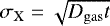 (Ciesla 2010). A steady state is reached if σX = H, the scale height of the disk, at which point a constant abundance is reached. As such we can estimate the time needed for vertical mixing. For a self-similar disk, this time scale becomes:
 (36)
(36)
If a similar mixing speed (α) is assumed for the radial and vertical processes, then vertical mixing should happen well within the lifetime of the disk for locations near the CO2 iceline.
Given these uncertainties, a simple constant abundance up to a certain height has been chosen. However higher up in the disk, photodissociation by stellar radiation and processing by stellar X-rays become important. CO2 is removed in our model in the harshest environments (AV < 1 mag), but CO2 photodissociation is still possible in the upper disk regions where CO2 is included. The location and thickness of this layer is discussed in Sects. 5.2.5 and 5.2.6.
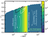 |
Fig. 8 2D CO2
abundance distribution from the |
5 Discussion
Viscous disk models including only freeze-out and desorption of CO2 predict a higher CO2 abundance than observed. This conclusion holds even for models without grain growth and radial drift. The discussion is divided into two sections, first the gas and grain surface chemistry is discussed to explore alternative chemical destruction routes. Subsequently physical effects are investigated, some of which also imply chemical effects to happen. Figure 11 shows the CO2 abundance structure in the disk with some of the mechanisms discussed here that could obtain agreement between observations and models.
5.1 Chemical processes
In the scenario that the CO2 released at the iceline is destroyed, an effective destruction rate of 10−11 s−1 or higher is required to match the observed and computed abundances. In Sects. 3.2.2 and 3.2.3 a number of known destruction processes for midplane CO2 were discussed, but none of these chemical processes is able to account for the destruction rate of 10−11 s−1.
5.1.1 Clues from high-mass protostars?
Our finding that a CO2 ice desorption model is inconsistent with CO2 gas-phase observations is not the first to do so. For high mass protostars Boonman et al. (2003) noted a similar disagreement between simple in-fall and desorption models, which predict CO2 gas-phase abundances around 10−5 whereas observations are more consistent with an abundance of ~10−7, a two orders of magnitude difference. Assuming that the CO2 ice sublimates and is destroyed within the dynamical time of 104 yr, a destruction rate of at least 10−11 s−1 is needed for protostars as well, of the same order as the rate needed in disks. If the CO2 destruction mechanism is similar in both types of sources, then this would most likely be a chemical destruction mechanism with no or a weak dependence on total density since densities in protostellar envelopes are orders of magnitude lower than in the inner disk midplanes and the physical environments are very different. However, as argued below the existence of such a chemical pathway is unlikely, except for destruction by UV photons or X-rays.
5.1.2 Alternative gas phase destruction routes
Here we investigate whether a chemical pathway could be missing in the chemical networks. Since ion-molecule reactions initiated by He+ have already been discarded, the assumption is that this destruction comes from a neutral-neutral reactive collision. The rate for a two-body reaction can be written as:
 (37)
(37)
where ngas is the gas number density, k2- body is the two-body reaction rate coefficient, xX is the abundance of the collision partner and fX is the branching ratio to any product that does not cycle back to CO2 . Near the iceline densities are around 1013 cm−3, a typical rate coefficient for a barrier-less neutral-neutral reaction is around 10−11 cm3 s−1. As such the partner abundance needs to be higher than 10−13 to destroy CO2 at a fast enough rate. The only species that have a nearly barrier-less reaction with CO2 in either the UMIST (McElroy et al. 2013) or KIDA (Wakelam et al. 2012) databases are C, CH2 and Si. Reaction rates for CO2 with C to form two CO molecules and with CH2 to form CO + H2CO are 10−15 cm3 s−1 and 3.9 × 10⁻¹⁴ cm3 s−1 (Tsang & Hampson 1986), however, both rates are high temperature estimates and extrapolated to low temperatures (Hébrard et al. 2009). The rate for CO 2 + Si →CO + SiO has been measured at room temperature to be 1.1 × 10⁻¹¹ cm3 s−1 (Husain & Norris 1978), McElroy et al. (2013) assume a small energy barrier of 282 K, in line with the high temperature measurements. Other species in the databases that have an exothermic reaction with CO2 are CH and N; both of these reactions are thought to have a barrier of 3000 and 1710 K respectively (Mitchell 1984; Avramenko & Krasnen’kov 1967). Other neutral-neutral reactions in the chemical networks are highly endothermic, for example CO 2 + S →CO + SO is endothermic by ~20 000 K (Singleton & Cvetanovic 1988), effectively nullifying this reaction in the temperature range we are interested in.
C, CH2 and Si are, due to their high reactivity, only present in very low quantities in the gas-phase with abundances at the solver accuracy limit of 10−17 for C and CH2 , and 10−16 for Si and thus can hardly account for the destruction of a significant amount of CO2 unless it is possible to quickly reform the initial reactant from the reaction products. The reactions products, CO, H 2 CO and SiO, are again very stable, thus it is unlikely that these molecules quickly react further to form the initial reactants again. This means that the abundance of C, CH2 and Si will go down with time if more and more CO2 is added.
5.1.3 Alternative ice destruction routes
The low CO2 abundance observed could also be explained if CO2 is converted to other species while in the ice. Bisschop et al. (2007) report that CO2 bombarded with H does not lead to HCOOH at detectable levels in their experiments. There are no data available on grain surfaces reactions of CO2 ice with N, Si or C. If any of these reaction pathways were to destroy CO2 in the ice, they should be very efficient, ~99% conversion, but at the same time be able to explain the high CO2 ice abundances in comets. This quickly limits the temperature range in which these reactions can be efficient to 30–80 K.
In short, due to the high stability of CO2, only a handful of highly reactive radicals or atoms can destroy CO2 , whether in the gas or ice. None of these species is predicted to be abundant enough to quickly destroy the large flux of CO2 that is brought into the inner disk due to dynamic processes of CO2-containing icy grains.
5.2 Physical processes
The abundance profiles computed in this work all assume that the CO2 can move freely through the disk, both in radial and vertical directions, while being shielded from UV and X-ray radiation. It is also assumed that all CO2 ice sublimates at the CO2 iceline and that CO2 is highly abundant in the ice, as found in the ISM. Several physical processes could make these assumptions invalid. An important constraint is that due to the difference between the ice abundances (around 10−5) and the inferred gas abundance ( < 10−7) any process needs reduce the CO2 abundance in the infrared emitting layers by at least two orders of magnitude.
5.2.1 Impact of reduced turbulence
The currentmodels assume a standard viscously spreading and evolving disk with a constant α value. Magneto-hydrodynamical (MHD) simulations currently favour disks with strongly changing viscosity in radial and vertical directions (e.g. Gammie 1996; Turner et al. 2007; Bai & Stone 2013). In these simulations turbulence is only expected to be high at those locations where the ionisation fraction of the gas is also high, that is, the upper and outer regions of the disk. In the disk mid-plane the viscous α may be as low as 10−6 , especially if non-ideal MHD effects are taken into account. In this regime, radial and vertical mixing due to the turbulence becomes a very slow process, with mixing time-scales close to the disk lifetime. Laminar accretion through the midplane would still enrich the inner disk midplane with CO2 but the low vertical mixing would greatly reduce the amount of material that is lifted into the IR-emitting layers of the disk. A mixing time of 106 yr would imply an effective vertical α of 10−6 for a CO2 iceline at 10 AU (Eq. (36), Ciesla 2010). Note that this still means that CO2 is mixed upwards within 105 yr in the inner 1 AU, which would be visible as an added warmer component to the CO2 emission. Observations of another species created primarily on grains at high abundance, > 10−7, such as CH4, NH3 or CH3OH near their respective icelines can be used to rule out inefficient vertical mixing.
5.2.2 Trapping of CO2 in large solids
There are ways to trap a volatile in a less volatile substance and prevent or delay its sublimation to higher temperatures. One possibility is to lock up the CO2 inside the water ice. This can be done in the bulk of the amorphous ice, below the surface layers, or by the formation of clathrates in the water ice at the high midplane pressures. Even in the case that CO2 is completely trapped in H2O ice, CO2 still comes off the grain together with the H2O at the H2 O iceline. At this point the CO2 is in the gasphase and free to diffuse around in the disk. The strong negative abundance gradient outside the H2 O iceline will transport the CO2 outwards until the CO2 starts to freeze-out of its own accord at the CO2 iceline. This would still result in gas-phase abundances within the CO2 iceline close to the original icy CO2 abundances of the outer disk.
Spherical grains between 0.1 μm and 1 mm are coated with 102 to 1010 layers of water ice, respectively. In the case of small particles, with only 100 layers of ice, it is hard to imagine that the water traps a significant amount of CO2 . For the larger grains with a smaller relative surface area, however, the water ice could readily trap a lot of CO2 . In a fully mixed H2O and CO2 ice, the sublimation of CO2 from the upper 100 million ice layers will still keep the fraction of sublimated CO2 below 1%, however efficient grain fragmentation, such as assumed in our models, will expose CO2 rich layers allowing for the sublimation of more CO2. For small grains, clathrates may keep the CO2 locked-up in the upper layers to prevent sublimation. However, to trap a single CO2 molecule at least six H2O molecules are needed (Fleyfel & Devlin 1991).
For amorphous ices similar restrictions exists on the H2O to CO2 ratio for trapping CO2 in the water ice. For ices with a H2O to CO2 ratio of 5:1, CO2 desorption happens at the CO2 desorption temperature, only at a ratio of 20:1 is the CO2 fully trapped within the H2O ice (Sandford & Allamandola 1990). Collings et al. (2004) show that the majority of the trapped CO2 desorbs at temperatures just below the desorption temperature of H2O, due to the crystallization of water. Fayolle et al. (2011) note that the fraction of trapped CO2 also depends on the thickness of the ice. They are able to trap 65% of the CO2 in a 5:1 ice, which means that a significant fraction of the CO2 still comes of at the CO2 iceline.
Both of these mechanisms need to have all the CO2 mixed with water. For interstellar dust grains there is observational evidence that this is not the case: high quality Spitzer spectra indicate that CO2 is mixed in both the CO-rich layers of the ice as well as the H2 O-rich layers of the ice (Pontoppidan et al. 2008). Sublimation of CO from these mixed ices would create a CO2 rich layer around the mixed H2 O:CO2 inner layers.
Another option would be to lock the CO2 in the refractory material. We note however that the CO2 ice abundance is of the same order as the Mg, Fe and Si abundances (Asplund et al. 2009), as such it is unlikely that CO2 can be locked up in the refractory material without chemical altering that material, such as conversion into, for example, CaCO3 .
Measurements from 67P/Churyumov-Gerasimenko indicate that even a kilometre-sized object outgasses CO2 at 3.5 AU distance (Hässig et al. 2015). For larger objects, CO2 retention might be possible, butlocking up 99% of the CO2 ice in these bodies seems highly unlikely.
5.2.3 Trapping icy grains outside of the iceline
It is possibleto stop the CO2 from sublimating if the CO2 ice never reaches the CO2 iceline, for example by introducing a dust trap (van der Marel et al. 2013). Stopping the CO2 ice from crossing the iceline would also mean stopping the small dust from crossing the iceline. This would lead to fast depletion of the dust in the inner disk, creating a transition disk, although some small dust grains can still cross the gap (Pinilla et al. 2016). Indeed, most disks for which CO2 has been measured have strong near- and mid-infrared continuum emission, indicating that the inner dust disks cannot be strongly depleted. Furthermore, measurements by Kama et al. (2015) show that for Herbig Ae stars, the accreting material coming from a full disk has a refractory material content close to the assumed ISM values even though these disks have no detectable infrared CO2 emission with Spitzer (Pontoppidan et al. 2010).
5.2.4 Shocks
For high-mass protostars, Charnley & Kaufman (2000) proposed that C-shocks with speeds above 30 km s−1 passing through the region within the CO2 iceline could account for the low observed CO2 abundance. Dense C-shocks can elevate temperatures above 1000 K and create free atoms such as H, N and C, so all of the CO2 in the shocked layer can then be efficiently converted to H2O and CO. At the higher densities in disks, lower velocity shocks can reach the same temperature. For example, Stammler & Dullemond (2014) calculate that a 5 km s−1 shock would reach temperatures upwards of 1000 K in the post shock gas. If shocks with such speeds occur in disks as well this could be an explanation for the low CO2 abundance. However, assuming the shock only destroys gas-phase CO2, not the ice, shocks must happen at least once every 3 × 10³ yr (1∕10−11 s−1) and the shock speeds have to be of the order of the Keplerian velocity.
These nebular shocks have been invoked to explain the ubiquitous chondrules found in meteorites. For these chondrules to form, dense gas needs to be flash heated, so that grains can evaporate and quickly reform as the gas cools (Hewins et al. 2005). Desch & Connolly (2002) proposed that a slow shock (7 km s−1 ) in the dense midplane can heat up the gas to temperature around 2000 K, enough to start sublimation (see also Stammler & Dullemond 2014). In the case of efficient cooling, it takes the gas a few minutes to cool, but this would be enough for the CO 2 + H →CO + OH reaction to significantly reduce the CO2 abundance. Slower shocks, with low cooling rates would also be able to destroy CO2 efficiently, as long as temperatures of 750 K are reached (see Fig. B.1). To effectively destroy CO2, these shocksneed to affect the entire inner disk at least once every few thousand years. Each shock could then also induce chondrule formation. There is evidence that chondrules went through multiple creation events, but the frequency of these events is currently not constrained (Ruzicka et al. 2008; Desch et al. 2012).
Further out in the disk, shocks can sputter ices, including CO2 ice, from the grains (Charnley & Kaufman 2000). However, sputtering does not necessarily destroy the CO2 . Moreover, full destruction of ices by shocks is unlikely since CO2 needs to survive in the comet formation regions of the disk.
5.2.5 UV-dominated layers
The inner disk chemical models by Walsh et al. (2015) show that there is a surface layer in the disk where UV destruction becomes important resulting in abundances of 10−8–10−7. Depending on the time-scale of the chemical processes and the extent of this layer, it may be optically thick in the 12 CO2 infrared lines. This means that low abundances of CO2 will be measuredin 12CO2 irrespective of the amount of sublimating CO2 ice in the midplane. If this UV-dominated layer is not too thick, 13 CO2 could still have an imprint of the deeper, more abundant CO2 that is coming from the iceline. On the other hand, if this layer is thick enough that even 13 CO2 becomes optically thick to its own radiation, then the more abundant CO2 sublimating from the iceline would be hidden from our view (see Figs. 10 and 12). This would happen at CO2 columns larger than 1018 cm−2.
The (vertical) thickness of the photon dominated layer is very dependent on the UV flux and dust opacity in the upper layers of the disk. For a disk that has only small grains ( < 1 μm) in the upperatmosphere, the UV opacity is high. In this case the UV dominated layer only contains a short column of gas, and thus CO2 (Fig. 13). Observations of such a disk would lead to the spectra as presented in Sect. 4.5. If it is assumed that grains have grown to mm sizes, even in the upper atmosphere, then the UV can penetrate a lot deeper. This leads to a larger column of UV dominated gas and that could hide the high abundance CO2 in the midplane, if the CO2 in this layer becomes optically thick to its own IR radiation or if the dust becomes optically thick at IR wavelengths in the UV dominated layer. The first scenario is sketched in panel C of Fig. 11. To probe the midplane CO2 abundance one would need to observe disks with a lot of small grains in the upper atmosphere, preferably around UV weak sources such that the CO2 column in the UV dominated layer is minimised.
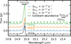 |
Fig. 9 Spectra 12CO2 and 13 CO2 for models with different destruction rates at a spectral resolving power R = 2200 appropriate for JWST-MIRI. The abundance floor is taken to be 10−8. The black line shows the model results for a constant abundance as used in Bosman et al. (2017). The regions were the Q-branch flux is extracted is shown in the black lines. The 13CO2 Q-branch is blended with the 12CO2 P(23) line. The neighbouring P(21) line is indicated. Note that the models with destruction rates of 10−11 and 10−10 s−1 are indistinguishable in their 12CO2 spectra. |
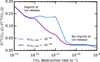 |
Fig. 10 Flux ratios of the 13CO2 and 12 CO2 Q-branches, determined by integrating the region shown in Fig. 9. The 13 CO 2 Q-branch flux is corrected for the emission of the P(23) line by subtraction of the neighbouring P(21) line flux. |
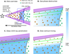 |
Fig. 11 Schematic representation of the CO2 abundance near the iceline in the r–z plane. Panels B, C and D approximately represent the top half of the blue box in panel A. The straight green lines denote the τ = 1 surface for 12CO2 (solid) and 13CO2 (dashed). Panels B, C and D: the abundance structure under different mechanism to explain the difference in CO2 abundance between the predictions of the viscous model and the IR observations. Panel B: the case for a constant gas-phase destruction rate due to some as yet unidentified process (Sect. 4.4). Panel C: the abundance structure for deep UV/X-ray penetration (Sects. 5.2.5 and 5.2.6). In more extreme cases, the 13 CO 2 τ = 1 surface can also be in the UV/X-ray dominated region. Panel D: the abundance structure for negligible vertical mixing (Sect. 5.2.1). Image not to scale. |
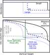 |
Fig. 12 Schematic of the vertical CO2 abundance (top panel) and upwards column (bottom panel) as function of disk height. Three different cases areshown in solid black, dashed dark blue and dotted blue lines. The black line shows the case for shallow UV or X-ray penetration, in this case an abundance similar to the midplane CO2 abundance will be measured. The dashed dark blue line shows a slightly deeper penetration of radiation, in which case a lower CO2 abundance will be inferred from the observations because the gas is optically thick and hiding the higher abundance deeper into the disk. The dotted blue line shows the case of deep penetration. In this case a low CO2 abundance will be inferred due to the dust hiding the bulk of the CO2. The vertical lines in the upper panel show where the disk becomes optically thick to CO2 lines, the solid and dashed grey line, show where the gas becomes optically thick for the small and intermediate PDR or XDR respectively, the green dotted line shows where the dust becomes optically thick, which is above where the gas becomes optically thick for the large PDR or XDR. |
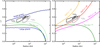 |
Fig. 13 Left: depth into the disk to which UV can destroy CO2 at a rate of 10−11 s−1 for a disk with an upper disk gas-to-dust ratio of 1000 and large grains (cyan) and small grains (blue). The black and grey contours show the area from which 25% and 75% of the emission of 12 CO 2 and 13 CO2 respectively originates. The green lines show the dust τ = 1 surface at 15 μm for the large grains (up to 1 mm, dark green) and small grains (up to 1 μm, light green) respectively. The UV photo destruction rate has a stronger dependence on the grain size distribution than this μm dust photosphere. Right: depth into the disk to which X-rays can destroy CO2 at a rate of 10−11 s−1 for different stellar X-ray luminosities (LX in erg s−1 ). The black and grey contours show the area from which 25% and 75% of the emission of 12 CO 2 and 13 CO2 respectively is coming from. The green line shows the dust τ = 1 surface at 15 μm for the large grains (up to 1 mm). |
5.2.6 X-ray induced dissociation
T-Tauri stars are known to have strong X-ray emission 1028 –1034 erg s−1 (Feigelson et al. 2002). These X-rays can ionise the gas and create a local UV field in the same way as cosmic-rays, destroying molecules in the gas (see, for example, the models by Stäuber et al. 2005, for high mass protostars). As X-rays are more quickly attenuated than the higher energy cosmic-rays, they are not efficient in destroying CO2 in the disk midplane, however, X-rays do penetrate further into the disk atmosphere than UV photons. Thus, X-rays can help in decreasing the CO2 abundance in the atmosphere of the disk, especially if hard X-ray flare, such are thought to occur in TW Hya are common in other T-Tauri stars as well (Kastner et al. 2002; Cleeves et al. 2015, 2017).
For our specific DALI model, a total X-ray flux of 1030 erg s−1, emitted as a 107 K black body, would have a destruction rate of 10−11 s−1 in most of the 12CO2 emitting region and could thus have an effect on the 12CO2 fluxes (Fig. 13). A total X-ray flux of 1032 erg s−1 would be needed to have the same destruction rate in most of the 13 CO2 emitting region. Thus, a source that has a time-averaged X-ray luminosity > 1030 erg s−1 could show a low CO2 abundance in the atmosphere and have a higher abundance underneath. If the X-ray luminosity of the source is lower than 1032 erg s−1, this should be reflected in the 13CO2 measurement. Note however that the X-rays do not reach into the midplane mass reservoir. Since the vertical transport for a fully viscous disk is orders of magnitude faster than the radial transport, the replenishment rate of CO2 in the upper layers due to mixing from the midplane would also be faster. Thus, these X-ray luminosities should be considered as lower limits. Most disk hosting stars do not have high enough X-ray luminosities to destroy CO2 efficiently (Bustamante et al. 2016), but X-ray destruction of CO2 in the surface layers can be an explanation in some sources and lead to similar effects as for the case of UV, such as the CO2 IR lines becoming optically thick in the X-ray dominated region.
6 Summary and conclusions
We have presented a model for the transport of major gas and ice species. This model predicts that transport of ices from the outer disk towards the inner disk can have a significant effect on the abundance of species in the inner disk. Radial transport is predicted to be so efficient, that even in the case without any radial drift, the modelled CO2 abundance in the inner disk is orders of magnitude higher than the currently available observations of disks. As such CO2 cannot be directly used to trace the mass transport rate. The presence of dust in disks older than a Myr does imply that the mass transport rate of dust cannot be larger than 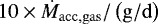 . This is inconsistent with the pebble-sized dust observed in disks.
To reconcile model and observation CO2 abundances,either the midplane CO2 needs to bedestroyed by some physical or chemical mechanism, or the CO2 abundance in the upper layers needs to be decoupled from the CO2 abundance in the midplane. This can be achieved by preventing vertical CO2 cycling, hiding the CO2 under the dust IR photosphere or by the creating a low abundance CO2 column that is optically thick in a UV or X-ray dominated layer. We can summarize this work with the following conclusions.
-
Accretion flow and diffusion equilibrate the inner disk CO2 gas abundance with the high outer disk CO2 ice abundance of ~10−5 in less than 1 Myr for α > 10−3 (Sect. 4.1).
-
For any disk that retains its dust on the same time-scale as it retains the gas, dust diffusion processes dominate over radial drift (Sect. 4.2 and Appendix C).
-
If dust can grow efficiently and drift inwards, both CO2 and H2O will be enhanced above the outer disk ice abundance as long as the dust is drifting inwards with a mass flux more than 1% of that of the gas,
 (Sect. 4.4).
 -
A physical or chemical process that would induce a vertically averaged CO2 destruction rate of at least 10−11 s−1 ( < 103 yr) is necessary to produce 12CO2 fluxes that are consistent with the current observations of disks (Sect. 4.5).
-
Within the current chemical networks, there are no paths to destroy CO2 fast enough without invoking strong X-ray or UV-fluxes or elevated cosmic ray fluxes. Especially at temperatures between 60 and 150 K, destroying CO2 is extremely difficult in the current chemical networks since the formation of CO2 is strongly favoured over the production of H2O in that temperature range. Above 300 K CO2 destruction pathways exists, but they only become efficient enough at temperatures above 750 K (Sects. 3.2, 5.1 and Appendix B).
-
Shocks could raise temperatures enough to destroy CO2 efficiently, but effectively lowering the CO2 abundance would require the entire inner 10 AU of the disk to be processed by a shock every 103 yr.
-
Trapping CO2 in water ice seems unlikely and is not expected to lower the inner disk gaseous CO2 abundance significantly. Trapping the grains before they cross the iceline efficiently enough to lower CO2 abundances in the inner disk would quickly create a transition disk (Sects. 5.2.2 and 5.2.3).
-
Deep penetration of UV and strong X-ray fluxes can lower the CO2 abundance in the 12CO2 emitting region. This can happen if grains in the disk atmosphere have grown to mm sizes and the central source has enough UV luminosity ( > 1027 erg s−1, about 0.1% of the solar UV). Likewise sources that have an X-ray luminosity greater than 1030 erg s−1 efficiently destroy CO2 in a large part of the IR emitting region. If the UV or X-ray dominated region does not reach down to the dust 15 μm τ = 1 surface, 13CO2 can still contain a information on the amount of sublimated CO2.
-
A high ratio of the 13CO2 Q-branch flux over the 12CO2 Q-branch flux ( >0.05), can hint at an contribution of sublimating CO2 at the iceline. Sublimating CO2 is, however, not the only way to get high flux ratios. A more complete, source specific analysis would be needed to exclude other possibilities (Sect. 4.5).
In summary, to explain the discrepancy between our models and observations, we either need to invoke frequent shocks in the inner 10 AU, or need to hide the abundant midplane CO2 from our view. This can be due to very inefficient mixing or due to deep UV and/or X-ray penetration. In the case of UV penetration, this would imply efficient grain growth and settling, in the case of X-rays, this would be stronger than measured X-ray fluxes for most sources, or frequent X-ray flares. The key to hiding the mid-plane CO2 is that the low abundance CO2 in the upper layers has a high enough column density to become optically thick to its own IR radiation. Trapping the CO2 on the grains, or destroying it in the gas phase near the iceline at ambient temperatures is strongly disfavoured.
Is CO2 a special case in terms of discrepancy between models and observations? Modelling and observations of other molecules abundant in ices, such as NH3 and CH4 , may be used to test whether a chemical or physical reason is the origin of the current discrepancy. Ultimately, such data can constrain the mass flow of solids if the chemical composition of the surface layers is sufficiently representative of that in the midplane.
Acknowledgements
Astrochemistry in Leiden is supported by the European Union A-ERC grant 291141 CHEMPLAN, by the Netherlands Research School for Astronomy (NOVA), by a Royal Netherlands Academy of Arts and Sciences (KNAW) professor prize. Daniel Harsono, Stefano Facchini, Kees Dullemond and Til Birnstiel are thanked for insightful discussions and Catherine Walsh and Christian Eistrup for sharing and help with the gas-grain chemical network.
Appendix A UV dust cross sections
Figure A.1 shows the UV opacities and cross sections for different grain size distributions used in Sect. 3.2.2.
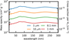 |
Fig. A.1 UV opacities and cross section of the dust for different sizes of the largest grains. The MRN power law slope is 3.5 for all cases. Growing grains from 1 μm to 1 mm hasmore than an order of magnitude effect on the opacities. |
Appendix B Chemical modelling
B.1 Gas-phase only models
To test the main CO2 destruction and formation processes, a small grid of chemical models was run. The network from Walsh et al. (2014) was used as basis and modified. The gas-phase chemical network is based on the UMIST 2012 network (McElroy et al. 2013). The network includes freeze-out and desorption. H2 formation on grains following Cazaux & Tielens (2004), which includes H2 formation at high temperatures. The grain-surface reactions included in the network were removed for this test. As the main interest is inthe midplane layers, the local UV and X-ray flux are assumed to be negligible. The cosmic ray rate is taken to be 10−17 s−1.
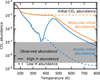 |
Fig. B.1 CO2 abundance from a gas-phase chemical network as function of temperature after 1 Myr of evolution. The density is 1012 cm−3. |
Initial molecular abundances for the chemical models.
Four series of models were run, two starting from “atomic” initial conditions (all species are in atomic form except for H2 ), the other two from “molecular” conditions (see Table B.1, the atomic initial conditions use the same elemental abundances as the used for the molecular test). For each set of initial conditions one set of models was run with H2 formation happening only on grains according to Cazaux & Tielens (2004) leading to an atomic H abundance of 10−4 with respect to H2 , while in the other set of models the additional H2 formation route at high temperature was added to keep the H abundance at 10−12 (1 cm−3 ). The density was kept constant at 1012 cm−3 and the temperature was varied between 150 and 800 K.
The CO2 abundances after 1 Myr of chemical evolution are presented in Fig. B.1. From this plot it can be gathered that there is no efficient destruction mechanism in the current gas-phase network until a temperature of ~450 K is reached.
For temperatures between 150 and 450 K, the different atomic H abundances do not significantly influence the results. The difference between the initial CO2 abundance and the CO2 abundance after 1 Myr in the molecular case can be explained by the destruction of CO2 and H2 O due to processes driven by cosmic rays, e.g. cosmic ray induced photo dissociation, and the reformation of CO2 from the fragments.
For models starting from atomic initial conditions the CO2 content decreases with increasing temperature as expected from the formation speeds of CO2 and H2 O in the model with a low H abundance, and this trend continues up to higher temperatures. The local minimum in the CO2 abundance at 350 K is dueto reactions with atomic N before the nitrogen is locked up in other species. When the atomic nitrogen abundance is high, CO2 reacts with N to form CO and NO, NO is then further processed to H2O, releasing a N in the process. This significantly slows down the build-up of CO2 when both O and OH are available in the gas-phase in high abundances.
In the models with a high H abundance, reactions with atomic hydrogen become important starting at 350 K. This process, which is slightly more efficient for H2O than for CO2 , together with the reformation of H2O and CO2 from the resulting OH, sets the equilibrium at high temperature. The abundance of H2 O as function of temperature is fairly constant, at 10−4, and thus the CO2 abundance decreases towards the highest temperature, as expected from the formation rate ratio given in Fig. 1. The difference between the CO2 abundance at high temperature in the case of atomic and molecular abundance can be explained by the lower CO abundance in the case of atomic initial conditions.
For the models with a low H abundance, CO2 is not efficiently destroyed by H at high temperatures so the CO2 abundance is nearly constant as function of temperature. From this parameter exploration we can conclude that CO2 can only be effectively destroyed by radicals like H and N and that this is only efficient if these are available at high abundances > 10−6. For the model beginning with atomic abundances the low temperature dependence of the abundance is similar to the high H abundance case. Above temperatures of 400 K differences start to be noticeable. The CO2 abundance does not increase with temperature as it does in the case of high H abundance. This is due to a similar process as in the high H model around 350 K. All the CO2 that is formed when oxygen is not locked up in water is quickly destroyed by atomic H and N, when atomic H and N have settled to low enough abundances that CO2 can survive, all the O is already locked up in other species, mostly H2O and CO leaving no extra O to form CO2. The small amount of CO2 that is in the gas-phase is mostly created by cosmic ray induced destruction of H2 O. The decreasing abundance towards high temperatures is due to the increasingly efficient reformation of H2 O after destruction due to cosmic rays.
B.2 Grain surface chemistry between the H2O and CO2 icelines
Section B.1 investigates the gas-phase chemistry of CO2 in the region within the H2 O iceline, that is, above 150K. In this region all species will be primarily in the gas-phase and grain surface chemistry is thus expected to be less important. Between theCO2 and H2 O icelines The efficiency of the destruction of gaseous CO2 is estimatedby investigating the chemical pathways in a full chemical model. The network from Walsh et al. (2014) and Eistrup et al. (2016) was used. A point model representative for the conditions between the H2 O and CO2 iceline was run. The number density used is 1013 cm−3, the temperature 100 K and the cosmic ray ionisation rate 10−17 s−1. There was no external UV in our model. After running the model for 1 Myr to get equilibrium abundances of atomic and ionised species, the chemical pathways of oxygen carrying species are examined.
For each oxygen carrying molecule that could be created from a destruction of CO2 , we define the destruction efficiency as the fraction the oxygen atoms that is incorporated into a stable molecule, for which we take that a cosmic ray induced process is needed to destroy the molecule. Here, pathways leading to incorporation of oxygen into CO are neglected, as these pathways are dominated by the availability of atomic C, which must originate from an other CO molecule. Pathways towards CO are generally very minor. Destruction efficiencies are tabulated in Table B.2.
Chemical pathways from molecules possibly created by the destruction of CO2 .
From the efficiencies it can be seen that direct ionisation or protonation of CO2 is not an effective way to destroy itsince CO2 will be reformed from the products in most cases. Only if an oxygen atom can be removed from the central carbon, is there a chance that the oxygen will be locked up into something other than CO2 . In these cases the efficiency is 27% (for OH) or higher. Appendix C:
Apppendix C Viscous evolution and grain growth
Figures C.1 through C.9 show model results for the model with grain growth and radial drift, but without any destruction rate. α values of 10−2, 10−3 and 10−4 are shown, fragmentation velocities of 1, 10 and 100 m s−1 are used. The features seen in ice abundance for the higher fragmentation velocity models is due to a numerical instability in the grain growth algorithm, this does not influence our results.
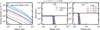 |
Fig. C.1 Time evolution series for a model with grain growth. This model assumes an α of 10−2 . The fragmentation velocity for this model is 1 m s−1. Panels as in Fig. 3. |
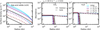 |
Fig. C.2 Time evolution series for a model with grain growth. This model assumes an α of 10−2 . The fragmentation velocity for this model is 1 m s−1. Panels as in Fig. 3. |
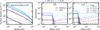 |
Fig. C.3 Time evolution series for a model with grain growth. This model assumes an α of 10−2 . The fragmentation velocity for this model is 1 m s−1. Panels as in Fig. 3. |
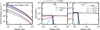 |
Fig. C.4 Time evolution series for a model with grain growth. This model assumes an α of 10−3 . The fragmentation velocity for this model is 1 m s−1. Panels as in Fig. 3. |
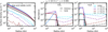 |
Fig. C.5 Time evolution series for a model with grain growth. This model assumes an α of 10−3 . The fragmentation velocity for this model is 10 m s−1. Panels as in Fig. 3. |
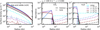 |
Fig. C.6 Time evolution series for a model with grain growth. This model assumes an α of 10−3 . The fragmentation velocity for this model is 100 m s−1. Panels as in Fig. 3. |
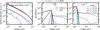 |
Fig. C.7 Time evolution series for a model with grain growth. This model assumes an α of 10−4 . The fragmentation velocity for this model is 1 m s−1. Panels as in Fig. 3. |
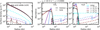 |
Fig. C.8 Time evolution series for a model with grain growth. This model assumes an α of 10−4 . The fragmentation velocity for this model is 10 m s−1. Panels as in Fig. 3. |
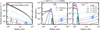 |
Fig. C.9 Time evolution series for a model with grain growth. This model assumes an α of 10−4 . The fragmentation velocity for this model is 100 m s−1. Panels as in Fig. 3. |
References
- Adams, N. G., & Smith, D. 1976, J. Phys. B: At. Mol. Phys., 9, 1439 [NASA ADS] [CrossRef] [Google Scholar]
- Agúndez, M., Cernicharo, J., & Goicoechea, J. R. 2008, A&A, 483, 831 [NASA ADS] [CrossRef] [EDP Sciences] [Google Scholar]
- Aikawa, Y., & Herbst, E. 1999, A&A, 351, 233 [NASA ADS] [Google Scholar]
- Ali-Dib, M., Mousis, O., Petit, J.-M., & Lunine, J. I. 2014, ApJ, 785, 125 [NASA ADS] [CrossRef] [Google Scholar]
- Andrews, S. M., Wilner, D. J., Hughes, A. M., Qi, C., & Dullemond, C. P. 2009, ApJ, 700, 1502 [NASA ADS] [CrossRef] [Google Scholar]
- Anicich, V. G., Laudenslager, J. B., Huntress, Jr., W. T., & Futrell, J. H. 1977, J. Chem. Phys., 67, 4340 [NASA ADS] [CrossRef] [Google Scholar]
- Ansdell, M., Williams, J. P., van der Marel, N., et al. 2016, ApJ, 828, 46 [Google Scholar]
- Asplund, M., Grevesse, N., Sauval, A. J., & Scott, P. 2009, ARA&A, 47, 481 [NASA ADS] [CrossRef] [Google Scholar]
- Avramenko, L. I., & Krasnen’kov, V. M. 1967, Bull. Acad. Sci. USSR Div. Chem. Sci. (Engl. Transl.), 16, 501 [CrossRef] [Google Scholar]
- Bai, X.-N., & Stone, J. M. 2013, ApJ, 769, 76 [NASA ADS] [CrossRef] [Google Scholar]
- Baulch, D. L., Cobos, C. J., Cox, R. A., et al. 1992, J. Phys. Chem. Ref. Data, 21, 411 [NASA ADS] [CrossRef] [Google Scholar]
- Bergin, E. A., Cleeves, L. I., Gorti, U., et al. 2013, Nature, 493, 644 [NASA ADS] [CrossRef] [PubMed] [Google Scholar]
- Birnstiel, T., Dullemond, C. P., & Brauer, F. 2010, A&A, 513, A79 [NASA ADS] [CrossRef] [EDP Sciences] [Google Scholar]
- Birnstiel, T., Klahr, H., & Ercolano, B. 2012, A&A, 539, A148 [NASA ADS] [CrossRef] [EDP Sciences] [Google Scholar]
- Bisschop, S. E., Fuchs, G. W., van Dishoeck, E. F., & Linnartz, H. 2007, A&A, 474, 1061 [NASA ADS] [CrossRef] [EDP Sciences] [Google Scholar]
- Blum, J., & Wurm, G. 2008, ARA&A, 46, 21 [NASA ADS] [CrossRef] [EDP Sciences] [Google Scholar]
- Boogert, A. C. A., Gerakines, P. A., & Whittet, D. C. B. 2015, ARA&A, 53, 541 [Google Scholar]
- Boonman, A. M. S., van Dishoeck, E. F., Lahuis, F., & Doty, S. D. 2003, A&A, 399, 1063 [NASA ADS] [CrossRef] [EDP Sciences] [Google Scholar]
- Booth, R. A., Clarke, C. J., Madhusudhan, N., & Ilee, J. D. 2017, MNRAS, 469, 3994 [NASA ADS] [CrossRef] [Google Scholar]
- Bosman, A. D., Bruderer, S., & van Dishoeck, E. F. 2017, A&A, 601, A36 [NASA ADS] [CrossRef] [EDP Sciences] [Google Scholar]
- Brauer, F., Dullemond, C. P., & Henning, T. 2008, A&A, 480, 859 [NASA ADS] [CrossRef] [EDP Sciences] [Google Scholar]
- Bruderer, S. 2013, A&A, 559, A46 [NASA ADS] [CrossRef] [EDP Sciences] [Google Scholar]
- Bruderer, S., van Dishoeck, E. F., Doty, S. D., & Herczeg, G. J. 2012, A&A, 541, A91 [NASA ADS] [CrossRef] [EDP Sciences] [Google Scholar]
- Bruderer, S., Harsono, D., & van Dishoeck, E. F. 2015, A&A, 575, A94 [NASA ADS] [CrossRef] [EDP Sciences] [Google Scholar]
- Bustamante, I., Merín, B., Bouy, H., et al. 2016, A&A, 587, A81 [Google Scholar]
- Carr, J. S., & Najita, J. R. 2008, Science, 319, 1504 [NASA ADS] [CrossRef] [PubMed] [Google Scholar]
- Cazaux, S., & Tielens, A. G. G. M. 2004, ApJ, 604, 222 [NASA ADS] [CrossRef] [Google Scholar]
- Charnley, S. B., & Kaufman, M. J. 2000, ApJ, 529, L111 [NASA ADS] [CrossRef] [Google Scholar]
- Ciesla, F. J. 2010, ApJ, 723, 514 [NASA ADS] [CrossRef] [Google Scholar]
- Ciesla, F. J., & Cuzzi, J. N. 2006, Icarus, 181, 178 [NASA ADS] [CrossRef] [Google Scholar]
- Clarke, C. J., & Pringle, J. E. 1988, MNRAS, 235, 365 [NASA ADS] [CrossRef] [Google Scholar]
- Cleeves, L. I., Bergin, E. A., Qi, C., Adams, F. C., & Öberg, K. I. 2015, ApJ, 799, 204 [NASA ADS] [CrossRef] [Google Scholar]
- Cleeves, L. I., Bergin, E. A., Öberg, K. I., et al. 2017, ApJ, 843, L3 [NASA ADS] [CrossRef] [Google Scholar]
- Collings, M. P., Anderson, M. A., Chen, R., et al. 2004, MNRAS, 354, 1133 [NASA ADS] [CrossRef] [Google Scholar]
- Cridland, A. J., Pudritz, R. E., Birnstiel, T., Cleeves, L. I., & Bergin, E. A. 2017, MNRAS, 469, 3910 [NASA ADS] [CrossRef] [Google Scholar]
- Cyr, K. E., Sears, W. D., & Lunine, J. I. 1998, Icarus, 135, 537 [NASA ADS] [CrossRef] [Google Scholar]
- Debes, J. H., Jang-Condell, H., Weinberger, A. J., Roberge, A., & Schneider, G. 2013, ApJ, 771, 45 [NASA ADS] [CrossRef] [Google Scholar]
- Desch, S. J., & Connolly, Jr., H. C. 2002, Meteor. Planet. Sci., 37, 183 [NASA ADS] [CrossRef] [Google Scholar]
- Desch, S. J., Morris, M. A., Connolly, H. C., & Boss, A. P. 2012, Meteor. Planet. Sci., 47, 1139 [NASA ADS] [CrossRef] [Google Scholar]
- Desch, S. J., Estrada, P. R., Kalyaan, A., & Cuzzi, J. N. 2017, ApJ, 840, 86 [NASA ADS] [CrossRef] [Google Scholar]
- Draine, B. T. 2003, ApJ, 598, 1017 [NASA ADS] [CrossRef] [Google Scholar]
- Draine, B. T.,& Lee, H. M. 1984, ApJ, 285, 89 [Google Scholar]
- Drozdovskaya,M. N., Walsh, C., van Dishoeck, E. F., et al. 2016, MNRAS, 462, 977 [NASA ADS] [CrossRef] [Google Scholar]
- Eistrup, C., Walsh, C., & van Dishoeck, E. F. 2016, A&A, 595, A83 [NASA ADS] [CrossRef] [EDP Sciences] [Google Scholar]
- Fayolle, E. C., Öberg, K. I., Cuppen, H. M., Visser, R., & Linnartz, H. 2011, A&A, 529, A74 [NASA ADS] [CrossRef] [EDP Sciences] [Google Scholar]
- Feigelson, E. D., Broos, P., Gaffney, III, J. A., et al. 2002, ApJ, 574, 258 [NASA ADS] [CrossRef] [Google Scholar]
- Fleyfel, F., & Devlin, J. P. 1991, J. Phys. Chem., 95, 3811 [CrossRef] [Google Scholar]
- Fraser, H. J., Collings, M. P., McCoustra, M. R. S., & Williams, D. A. 2001, MNRAS, 327, 1165 [NASA ADS] [CrossRef] [Google Scholar]
- Gammie, C. F. 1996, ApJ, 457, 355 [NASA ADS] [CrossRef] [Google Scholar]
- Gredel, R., Lepp, S., & Dalgarno, A. 1987, ApJ, 323, L137 [NASA ADS] [CrossRef] [Google Scholar]
- Gundlach, B., & Blum, J. 2015, ApJ, 798, 34 [NASA ADS] [CrossRef] [Google Scholar]
- Hartmann, L., Calvet, N., Gullbring, E., & D’Alessio, P. 1998, ApJ, 495, 385 [NASA ADS] [CrossRef] [Google Scholar]
- Hässig, M., Altwegg, K., Balsiger, H., et al. 2015, Science, 347 [Google Scholar]
- Heays, A. N., Bosman, A. D., & van Dishoeck, E. F. 2017, A&A, 602, A105 [NASA ADS] [CrossRef] [EDP Sciences] [Google Scholar]
- Hébrard, E., Dobrijevic, M., Pernot, P., et al. 2009, J. Phys. Chem. A, 113, 11227 [CrossRef] [PubMed] [Google Scholar]
- Hewins, R. H., Connolly, Jr., H. C., Lofgren, G. E., & Libourel, G. 2005, in Chondrites and the Protoplanetary Disk, eds. A. N. Krot, E. R. D. Scott, & B. Reipurth, ASP Conf. Ser., 341, 286 [NASA ADS] [Google Scholar]
- Husain, D., & Norris, P. E. 1978, Chem. Phys. Lett., 53, 474 [NASA ADS] [CrossRef] [Google Scholar]
- Johansen, A., & Lambrechts, M. 2017, Annu. Rev. Earth Planet. Sci., 45 [Google Scholar]
- Kama, M., Folsom, C. P., & Pinilla, P. 2015, A&A, 582, L10 [NASA ADS] [CrossRef] [EDP Sciences] [Google Scholar]
- Kastner, J. H., Huenemoerder, D. P., Schulz, N. S., Canizares, C. R., & Weintraub, D. A. 2002, ApJ, 567, 434 [NASA ADS] [CrossRef] [Google Scholar]
- Krijt, S., & Ciesla, F. J. 2016, ApJ, 822, 111 [NASA ADS] [CrossRef] [Google Scholar]
- Krijt, S., Ormel, C. W., Dominik, C., & Tielens, A. G. G. M. 2016, A&A, 586, A20 [NASA ADS] [CrossRef] [EDP Sciences] [Google Scholar]
- Lambrechts, M., & Johansen, A. 2012, A&A, 544, A32 [Google Scholar]
- Le Roy, L., Altwegg, K., Balsiger, H., et al. 2015, A&A, 583, A1 [Google Scholar]
- Madhusudhan, N., Knutson, H., Fortney, J. J., & Barman, T. 2014, in Protostars and Planets VI, eds. H. Beuther, R. Klessen, C. Dullemond, & T. Henning (University of Arizona Press, Tucson), 739 [Google Scholar]
- Manara, C. F., Rosotti, G., Testi, L., et al. 2016, A&A, 591, L3 [NASA ADS] [CrossRef] [EDP Sciences] [Google Scholar]
- Markwick, A. J., Ilgner, M., Millar, T. J., & Henning, T. 2002, A&A, 385, 632 [NASA ADS] [CrossRef] [EDP Sciences] [Google Scholar]
- Mauclaire, G., Derai, R., & Marx, R. 1978, Int. J. Mass Spectrom. Ion Phys., 26, 289 [Google Scholar]
- McClure, M. K., Bergin, E. A., Cleeves, L. I., et al. 2016, ApJ, 831, 167 [NASA ADS] [CrossRef] [Google Scholar]
- McElroy, D., Walsh, C., Markwick, A. J., et al. 2013, A&A, 550, A36 [NASA ADS] [CrossRef] [EDP Sciences] [Google Scholar]
- Meijerink, R., Pontoppidan, K. M., Blake, G. A., Poelman, D. R., & Dullemond, C. P. 2009, ApJ, 704, 1471 [NASA ADS] [CrossRef] [Google Scholar]
- Miotello, A., van Dishoeck, E. F., Williams, J. P., et al. 2017, A&A, 599, A113 [NASA ADS] [CrossRef] [EDP Sciences] [Google Scholar]
- Mitchell, G. F. 1984, Astrophys. J. Suppl. Ser., 54, 81 [NASA ADS] [CrossRef] [Google Scholar]
- Morbidelli, A.,& Raymond, S. N. 2016, J. Geophys. Res., 121, 1962 [NASA ADS] [CrossRef] [Google Scholar]
- Noble, J. A., Congiu, E., Dulieu, F., & Fraser, H. J. 2012, MNRAS, 421, 768 [NASA ADS] [Google Scholar]
- Öberg, K. I., & Bergin, E. A. 2016, ApJ, 831, L19 [NASA ADS] [CrossRef] [Google Scholar]
- Ormel, C. W., & Cuzzi, J. N. 2007, A&A, 466, 413 [NASA ADS] [CrossRef] [EDP Sciences] [Google Scholar]
- Ormel, C. W., & Klahr, H. H. 2010, A&A, 520, A43 [NASA ADS] [CrossRef] [EDP Sciences] [Google Scholar]
- Ormel, C., Liu, B., & Schoonenberg, D. 2017, A&A, 604, A1 [NASA ADS] [CrossRef] [EDP Sciences] [Google Scholar]
- Pérez, L. M., Carpenter, J. M., Chandler, C. J., et al. 2012, ApJ, 760, L17 [NASA ADS] [CrossRef] [Google Scholar]
- Pinilla, P., Klarmann, L., Birnstiel, T., et al. 2016, A&A, 585, A35 [NASA ADS] [CrossRef] [EDP Sciences] [Google Scholar]
- Piso, A.-M. A., Öberg, K. I., Birnstiel, T., & Murray-Clay, R. A. 2015, ApJ, 815, 109 [NASA ADS] [CrossRef] [EDP Sciences] [Google Scholar]
- Pontoppidan, K. M., & Blevins, S. M. 2014, Faraday Discuss., 169, 49 [NASA ADS] [CrossRef] [Google Scholar]
- Pontoppidan, K. M., Boogert, A. C. A., Fraser, H. J., et al. 2008, ApJ, 678, 1005 [NASA ADS] [CrossRef] [Google Scholar]
- Pontoppidan, K. M., Salyk, C., Blake, G. A., et al. 2010, ApJ, 720, 887 [NASA ADS] [CrossRef] [Google Scholar]
- Pontoppidan, K. M., Blake, G. A., & Smette, A. 2011, ApJ, 733, 84 [NASA ADS] [CrossRef] [Google Scholar]
- Prasad, S. S., & Tarafdar, S. P. 1983, ApJ, 267, 603 [NASA ADS] [CrossRef] [Google Scholar]
- Ruzicka, A., Floss, C., & Hutson, M. 2008, Geochim. Cosmochim. Acta, 72, 5530 [NASA ADS] [CrossRef] [Google Scholar]
- Sandford, S. A., & Allamandola, L. J. 1990, Icarus, 87, 188 [NASA ADS] [CrossRef] [PubMed] [Google Scholar]
- Schoonenberg,D., & Ormel, C. W. 2017, A&A, 602, A21 [NASA ADS] [CrossRef] [EDP Sciences] [Google Scholar]
- Shakura, N. I., & Sunyaev, R. A. 1973, A&A, 24, 337 [NASA ADS] [Google Scholar]
- Singleton, D. L., & Cvetanovic, R. J. 1988, J. Phys. Chem. Ref. Data, 17, 1377 [NASA ADS] [CrossRef] [Google Scholar]
- Smith, I. W. M., Herbst, E., & Chang, Q. 2004, MNRAS, 350, 323 [NASA ADS] [CrossRef] [Google Scholar]
- Stammler, S. M., & Dullemond, C. P. 2014, Icarus, 242, 1 [NASA ADS] [CrossRef] [Google Scholar]
- Stammler, S. M., Birnstiel, T., Panić, O., Dullemond, C. P., & Dominik, C. 2017, A&A, 600, A140 [NASA ADS] [CrossRef] [EDP Sciences] [Google Scholar]
- Stäuber, P., Doty, S. D., van Dishoeck, E. F., & Benz, A. O. 2005, A&A, 440, 949 [NASA ADS] [CrossRef] [EDP Sciences] [Google Scholar]
- Stevenson, D. J., & Lunine, J. I. 1988, Icarus, 75, 146 [NASA ADS] [CrossRef] [Google Scholar]
- Takeuchi, T., & Lin, D. N. C. 2002, ApJ, 581, 1344 [NASA ADS] [CrossRef] [Google Scholar]
- Talbi, D., & Herbst, E. 2002, A&A, 386, 1139 [NASA ADS] [CrossRef] [EDP Sciences] [Google Scholar]
- Tan, J. C., Chatterjee, S., Hu, X., Zhu, Z., & Mohanty, S. 2016, IAU Focus Meeting, 29, 6 [Google Scholar]
- Tazzari, M., Testi, L., Ercolano, B., et al. 2016, A&A, 588, A53 [NASA ADS] [CrossRef] [EDP Sciences] [Google Scholar]
- Testi, L., Birnstiel, T., Ricci, L., et al. 2014, Protostars and Planets VI, eds. H. Beuther, R. Klessen, C. Dullemond, & T. Henning (University of Arizona Press, Tucson), 339 [Google Scholar]
- Trapman, L., Miotello, A., Kama, M., van Dishoeck, E. F., & Bruderer, S. 2017, A&A, 605, A69 [NASA ADS] [CrossRef] [EDP Sciences] [Google Scholar]
- Tsang, W., & Hampson, R. F. 1986, J. Phys. Chem. Ref. Data, 15, 1087 [NASA ADS] [CrossRef] [Google Scholar]
- Turner, N. J., Sano, T., & Dziourkevitch, N. 2007, ApJ, 659, 729 [NASA ADS] [CrossRef] [Google Scholar]
- Turner, N. J., Fromang, S., Gammie, C., et al. 2014, Protostars and Planets VI, eds. H. Beuther, R. Klessen, C. Dullemond, & T. Henning (University of Arizona Press, Tucson), 411 [Google Scholar]
- Umebayashi, T., & Nakano, T. 1981, PASJ, 33, 617 [NASA ADS] [Google Scholar]
- Umebayashi, T., & Nakano, T. 2009, ApJ, 690, 69 [NASA ADS] [CrossRef] [Google Scholar]
- van der Marel,N., van Dishoeck, E. F., Bruderer, S., et al. 2013, Science, 340, 1199 [NASA ADS] [CrossRef] [PubMed] [Google Scholar]
- Wakelam, V., Herbst, E., Loison, J.-C., et al. 2012, ApJS, 199, 21 [NASA ADS] [CrossRef] [Google Scholar]
- Walsh, C., Millar, T. J., Nomura, H., et al. 2014, A&A, 563, A33 [NASA ADS] [CrossRef] [EDP Sciences] [Google Scholar]
- Walsh, C., Nomura, H., & van Dishoeck, E. 2015, A&A, 582, A88 [NASA ADS] [CrossRef] [EDP Sciences] [Google Scholar]
- Weidenschilling, S. J. 1977, MNRAS, 180, 57 [NASA ADS] [CrossRef] [Google Scholar]
- Weingartner, J. C., & Draine, B. T. 2001, ApJ, 548, 296 [NASA ADS] [CrossRef] [Google Scholar]
- Wolf, S., & Voshchinnikov, N. V. 2004, Comput. Phys. Commun., 162, 113 [NASA ADS] [CrossRef] [Google Scholar]
- Youdin, A. N., & Lithwick, Y. 2007, Icarus, 192, 588 [NASA ADS] [CrossRef] [Google Scholar]
exoplanets.org as of 28 November 2017.
Cratering and bouncing are neglected for simplicity.
UV cross-sections can be found here: http://home.strw.leidenuniv.nl/ewine/photo/
All Tables
Gas-phase abundances assumed for the cosmic ray induced dissociation rate calculations.
All Figures
|
Fig. 1 Ratio of the CO2 to H2 O formation rate from a reaction of OH with CO and H2 respectively. Hydrogenation of OH to H2O dominates above 150 K. Formation times of CO2 and H2 O from OH are faster than the inner disk mixing time for all temperatures considered here. |
| In the text | |
|
Fig. 2 Dissociation rate of CO2
due to cosmic ray induced photons, for different dust size distributions. Solid lines are for condition inside of the
H2 O
iceline, dashed lines for conditions outside of the H2O
iceline. The efficiency multiplied by |
| In the text | |
|
Fig. 3 Time evolution series for a model without grain growth. This model assumes an α of 10−3 . Left: surface density of the gas (solid lines) and solids (dashed lines), the solid surface density is the sum of the dust and ice surface densities, it has been multiplied by a factor of 10 for visualization. Middle: abundance of CO2 . Right: abundance of H2O. |
| In the text | |
|
Fig. 4 Time evolution series for a model with grain growth. This model assumes an α of 10−3 . The fragmentation velocity for this model is 3 m s−1. Panels as in Fig. 3. |
| In the text | |
|
Fig. 5 Time evolution series for a model with grain growth. The fragmentation velocity for this model is 30 m s−1 and α = 10−3. The verticalscales are different from Figs. 3 and 4. Panels as in Fig. 3. |
| In the text | |
|
Fig. 6 Timeevolution series for a model without grain growth but with a constant destruction rate of gaseous CO2 of 10−11 s−1. This model assumes an α of 10−3 . Panels as in Fig. 3, but with different vertical scales. |
| In the text | |
|
Fig. 7 Abundance of CO2 as function of radii for models with different destruction rates of CO2. These modeluse α = 10−3 and uf = 0 m s−1 (left) and uf = 3 m s−1 (right). Abundance profiles after 1 Myr of evolution are shown. At this point the disk has reached a semi steady state. A destruction rate of at least 10−11 s−1 is needed to keep the averaged CO2 abundance below the observational limit. The iceline is further out for models with higher destruction rates as the destruction of gas-phase CO2 lowers the total abundance of CO2 within 10 AU where CO2 can sublimate. |
| In the text | |
|
Fig. 8 2D CO2
abundance distribution from the |
| In the text | |
|
Fig. 9 Spectra 12CO2 and 13 CO2 for models with different destruction rates at a spectral resolving power R = 2200 appropriate for JWST-MIRI. The abundance floor is taken to be 10−8. The black line shows the model results for a constant abundance as used in Bosman et al. (2017). The regions were the Q-branch flux is extracted is shown in the black lines. The 13CO2 Q-branch is blended with the 12CO2 P(23) line. The neighbouring P(21) line is indicated. Note that the models with destruction rates of 10−11 and 10−10 s−1 are indistinguishable in their 12CO2 spectra. |
| In the text | |
|
Fig. 10 Flux ratios of the 13CO2 and 12 CO2 Q-branches, determined by integrating the region shown in Fig. 9. The 13 CO 2 Q-branch flux is corrected for the emission of the P(23) line by subtraction of the neighbouring P(21) line flux. |
| In the text | |
|
Fig. 11 Schematic representation of the CO2 abundance near the iceline in the r–z plane. Panels B, C and D approximately represent the top half of the blue box in panel A. The straight green lines denote the τ = 1 surface for 12CO2 (solid) and 13CO2 (dashed). Panels B, C and D: the abundance structure under different mechanism to explain the difference in CO2 abundance between the predictions of the viscous model and the IR observations. Panel B: the case for a constant gas-phase destruction rate due to some as yet unidentified process (Sect. 4.4). Panel C: the abundance structure for deep UV/X-ray penetration (Sects. 5.2.5 and 5.2.6). In more extreme cases, the 13 CO 2 τ = 1 surface can also be in the UV/X-ray dominated region. Panel D: the abundance structure for negligible vertical mixing (Sect. 5.2.1). Image not to scale. |
| In the text | |
|
Fig. 12 Schematic of the vertical CO2 abundance (top panel) and upwards column (bottom panel) as function of disk height. Three different cases areshown in solid black, dashed dark blue and dotted blue lines. The black line shows the case for shallow UV or X-ray penetration, in this case an abundance similar to the midplane CO2 abundance will be measured. The dashed dark blue line shows a slightly deeper penetration of radiation, in which case a lower CO2 abundance will be inferred from the observations because the gas is optically thick and hiding the higher abundance deeper into the disk. The dotted blue line shows the case of deep penetration. In this case a low CO2 abundance will be inferred due to the dust hiding the bulk of the CO2. The vertical lines in the upper panel show where the disk becomes optically thick to CO2 lines, the solid and dashed grey line, show where the gas becomes optically thick for the small and intermediate PDR or XDR respectively, the green dotted line shows where the dust becomes optically thick, which is above where the gas becomes optically thick for the large PDR or XDR. |
| In the text | |
|
Fig. 13 Left: depth into the disk to which UV can destroy CO2 at a rate of 10−11 s−1 for a disk with an upper disk gas-to-dust ratio of 1000 and large grains (cyan) and small grains (blue). The black and grey contours show the area from which 25% and 75% of the emission of 12 CO 2 and 13 CO2 respectively originates. The green lines show the dust τ = 1 surface at 15 μm for the large grains (up to 1 mm, dark green) and small grains (up to 1 μm, light green) respectively. The UV photo destruction rate has a stronger dependence on the grain size distribution than this μm dust photosphere. Right: depth into the disk to which X-rays can destroy CO2 at a rate of 10−11 s−1 for different stellar X-ray luminosities (LX in erg s−1 ). The black and grey contours show the area from which 25% and 75% of the emission of 12 CO 2 and 13 CO2 respectively is coming from. The green line shows the dust τ = 1 surface at 15 μm for the large grains (up to 1 mm). |
| In the text | |
|
Fig. A.1 UV opacities and cross section of the dust for different sizes of the largest grains. The MRN power law slope is 3.5 for all cases. Growing grains from 1 μm to 1 mm hasmore than an order of magnitude effect on the opacities. |
| In the text | |
|
Fig. B.1 CO2 abundance from a gas-phase chemical network as function of temperature after 1 Myr of evolution. The density is 1012 cm−3. |
| In the text | |
|
Fig. C.1 Time evolution series for a model with grain growth. This model assumes an α of 10−2 . The fragmentation velocity for this model is 1 m s−1. Panels as in Fig. 3. |
| In the text | |
|
Fig. C.2 Time evolution series for a model with grain growth. This model assumes an α of 10−2 . The fragmentation velocity for this model is 1 m s−1. Panels as in Fig. 3. |
| In the text | |
|
Fig. C.3 Time evolution series for a model with grain growth. This model assumes an α of 10−2 . The fragmentation velocity for this model is 1 m s−1. Panels as in Fig. 3. |
| In the text | |
|
Fig. C.4 Time evolution series for a model with grain growth. This model assumes an α of 10−3 . The fragmentation velocity for this model is 1 m s−1. Panels as in Fig. 3. |
| In the text | |
|
Fig. C.5 Time evolution series for a model with grain growth. This model assumes an α of 10−3 . The fragmentation velocity for this model is 10 m s−1. Panels as in Fig. 3. |
| In the text | |
|
Fig. C.6 Time evolution series for a model with grain growth. This model assumes an α of 10−3 . The fragmentation velocity for this model is 100 m s−1. Panels as in Fig. 3. |
| In the text | |
|
Fig. C.7 Time evolution series for a model with grain growth. This model assumes an α of 10−4 . The fragmentation velocity for this model is 1 m s−1. Panels as in Fig. 3. |
| In the text | |
|
Fig. C.8 Time evolution series for a model with grain growth. This model assumes an α of 10−4 . The fragmentation velocity for this model is 10 m s−1. Panels as in Fig. 3. |
| In the text | |
|
Fig. C.9 Time evolution series for a model with grain growth. This model assumes an α of 10−4 . The fragmentation velocity for this model is 100 m s−1. Panels as in Fig. 3. |
| In the text | |
Current usage metrics show cumulative count of Article Views (full-text article views including HTML views, PDF and ePub downloads, according to the available data) and Abstracts Views on Vision4Press platform.
Data correspond to usage on the plateform after 2015. The current usage metrics is available 48-96 hours after online publication and is updated daily on week days.
Initial download of the metrics may take a while.