| Issue |
A&A
Volume 611, March 2018
|
|
|---|---|---|
| Article Number | A95 | |
| Number of page(s) | 17 | |
| Section | Extragalactic astronomy | |
| DOI | https://doi.org/10.1051/0004-6361/201731669 | |
| Published online | 12 April 2018 | |
Lyman-continuum leakage as dominant source of diffuse ionized gas in the Antennae galaxy★
1
Leibniz-Institut für Astrophysik Potsdam (AIP),
An der Sternwarte 16,
14482
Potsdam, Germany
e-mail: This email address is being protected from spambots. You need JavaScript enabled to view it.
2
Instituto de Astrofísica de Canarias (IAC),
38205
La Laguna, Tenerife, Spain
3
Universidad de La Laguna,
Dpto. Astrofísica,
38206
La Laguna, Tenerife, Spain
4
Université de Lyon, Univ. Lyon1, ENS de Lyon, CNRS, Centre de Recherche Astrophysique de Lyon UMR5574,
69230
Saint-Genis-Laval, France
5
Observatoire de Genève, Université de Genève,
51 Ch. des Maillettes,
1290 Versoix, Switzerland
6
Institut für Astrophysik,
Friedrich-Hund-Platz 1,
37077
Göttingen, Germany
7
Department of Physics, ETH Zürich,
Wolfgang-Pauli-Strasse 27,
8093
Zürich, Switzerland
8
Leiden Observatory, Leiden University,
PO Box 9513,
2300 RA,
Leiden, The Netherlands
9
Institut für Physik und Astronomie, Universität Potsdam,
Karl-Liebknecht-Str. 24/25,
14476
Golm, Germany
Received:
28
July
2017
Accepted:
13
December
2017
Abstract
The Antennae galaxy (NGC 4038/39) is the closest major interacting galaxy system and is therefore often studied as a merger prototype. We present the first comprehensive integral field spectroscopic dataset of this system, observed with the MUSE instrument at the ESO VLT. We cover the two regions in this system which exhibit recent star formation: the central galaxy interaction and a region near the tip of the southern tidal tail. In these fields, we detect HII regions and diffuse ionized gas to unprecedented depth. About 15% of the ionized gas was undetected by previous observing campaigns. This newly detected faint ionized gas is visible everywhere around the central merger, and shows filamentary structure. We estimate diffuse gas fractions of about 60% in the central field and 10% in the southern region. We are able to show that the southern region contains a significantly different population of HII regions, showing fainter luminosities. By comparing HII region luminosities with the HST catalog of young star clusters in the central field, we estimate that there is enough Lyman-continuum leakage in the merger to explain the amount of diffuse ionized gas that we detect. We compare the Lyman-continuum escape fraction of each HII region against emission line ratios that are sensitive to the ionization parameter. While we find no systematic trend between these properties, the most extreme line ratios seem to be strong indicators of density bounded ionization. Extrapolating the Lyman-continuum escape fractions to the southern region, we conclude that simply from the comparison of the young stellar populations to the ionized gas there is no need to invoke other ionization mechanisms than Lyman-continuum leaking HII regions for the diffuse ionized gas in the Antennae.
Key words: galaxies: interactions / galaxies: individual: NGC 4038, NGC 4039 / galaxies: ISM / ISM: structure / HII regions
FITS images and Table of HII regions are available at the CDS via anonymous ftp to cdsarc.u-strasbg.fr (130.79.128.5) or via http://cdsarc.u-strasbg.fr/viz-bin/qcat?J/A+A/611/A95 and at http://muse-vlt.eu/science/antennae/
© ESO 2018
1 Introduction
In the hierarchical paradigm of galaxy formation, interactions and merging are major events in galaxy evolution (White & Rees 1978; Lacey & Cole 1993). They create some of the strongest starburst galaxies that we know (Sanders & Mirabel 1996) and shape the galaxies we see today in the nearby Universe (Steinmetz & Navarro 2002; Conselice 2003). From a theoretical point of view, mergers occur by the thousands in cosmological simulations (Schaye et al. 2015; Vogelsberger et al. 2014). From the observational point of view, major mergers have been identified at intermediate to high-redshift (e.g., Tacconi et al. 2008; Ivison et al. 2012; Ventou et al. 2017). They are also being studied in the nearby Universe, often in galaxies classified as infrared-bright (luminous or ultra-luminous infrared galaxy, LIRG or ULIRG, Alonso-Herrero et al. 2010; Rich et al. 2011), highlighting aspects as diverse as central shocks (Monreal-Ibero et al. 2006) and tidal dwarf galaxies (Weilbacher et al. 2003). One has to study the most nearby mergers in detail and at high spatial resolution to be able to disentangle and characterize the different elements playing a role in their evolution, in order to be able to properly interpret the high-redshift cases.
In that sense, the Antennae (NGC 4038/39, Arp 244), one of the most spectacular examples of gas-rich major mergers, and at a distance of 22 ± 3 Mpc (Schweizer et al. 2008), the closest one, constitutes a desirable laboratory to study the interplay of gas and strong recent star formation during the merger evolution. The system has a solar or slightly super-solar metallicity (Bastian et al. 2009; Lardo et al. 2015) and not only exhibits one of the most violent star-forming events in the nearby Universe, forming a multitude of young, massive stellar clusters in the central merger (Whitmore et al. 2005, 2010; Bastian et al. 2006), but also shows a more quiescent star-formation mode at the end of the southern tidal tail (Hibbard et al. 2005). Being such a paradigmatic object, it has a long history of being the subject of tailored simulations (e.g., Toomre & Toomre 1972; Karl et al. 2010; Renaud et al. 2015) and being extensively observed at all wavelengths, from radio to X-rays (e.g., radio: Bigiel et al. 2015; Whitmore et al. 2014; far- and mid-infrared: Brandl et al. 2009; Schirm et al. 2014; near-infrared: Brandl et al. 2005; Mengel et al. 2005; optical: Whitmore et al. 2010; ultraviolet: Hibbard et al. 2005).
An image of the Antennae system is shown in Fig. 1. In this publication, we deal with data of two fields, the central field and a southern one, both of which are marked with continuum contours taken in the HST ACS image; the same continuum contours are used throughout this paper.
An important missing piece of information would be a spectroscopic optical mapping of the whole system, ideally at high spatial and spectral resolution, and covering as much of the optical spectral range as possible. Data taken with the GHαFaS instrument presented by Zaragoza-Cardiel et al. (2014) were a first step in this direction. They cover the main body of both galaxies at very good spectral resolution (8km s−1). However, these data were gathered with a Fabry–Perot instrument, covering only a narrow spectral range around Hα. On the other side, long-slit observations can address these points, but only at very specific locations in the system (like individual star clusters, e.g., Whitmore et al. 2005; Bastian et al. 2009). Data from an Integral Field Spectrograph (IFS) would provide both, large spectral coverage and spatial mapping. Bastian et al. (2006) nicely illustrate the potential of this technique: with only one set of observations, both the ionized gas and the stellar populations can be mapped and characterized, although they still map only a smallportion of the system.
The advent of the Multi Unit Spectroscopic Explorer (MUSE Bacon et al. 2010) at the 8 m Very Large Telescope (VLT), with a large field of view (1′ × 1′) and a wide spectral coverage (~4600… 9350 Å at R ~ 3000), is the next step to overcome the shortcomings of previous observations. This motivated us to perform a thorough optical spectrocopicmapping of the system. In this first paper of a series, we will present the survey and, in particular, address one specific question: Can the photons leaking from the HII regions in the system explain the detected diffuse component of the ionized gas?
The diffuse ionized gas (DIG, also called warm ionized medium, WIM) has proven to be ubiquitous in star-forming galaxies, including ours (see Mathis 2000; Haffner et al. 2009 for a review). Strong emission line ratios in DIGs differ from those found in HII regions. Typically, they present higher forbidden-to-Balmer line ratios (e.g., [S II]6717,6731/Hα, [N II]6584/Hα, [O I]6300/Hα; Hoopes & Walterbos 2003; Madsen et al. 2006; Voges & Walterbos 2006) than HII regions.
Several mechanisms have been proposed to explain the detection of DIG in other galaxies and the unusual line ratios of which the most prominent are: (a) Lyman-continuum (LyC; λ < 912 Å) photons leaking from HII regions (Zurita et al. 2002) into the interstellar medium. Part of the UV continuum is absorbed by the gas, leading to a harder ionizing spectrum (Hoopes & Walterbos 2003) which can at least partly explain the observed properties. (b) Shocks are another mechanism to change the line ratios (Dopita & Sutherland 1995), and these are also frequently observed in merging galaxies (Monreal-Ibero et al. 2010; Soto et al. 2012). However, they are not always observed in the same parts of the galaxy as the DIG or do not explain its observed properties (e.g., all line ratios at the same time; Fensch et al. 2016). Finally, (c) evolved stars have a hard UV spectrum that could explain the DIG (Zhang et al. 2017). This is most relevant for early-type galaxies (Kehrig et al. 2012; Papaderos et al. 2013). However, in starburst galaxies their contribution to the Lyman-continuum is likely negligible compared to hot stars in star-forming regions, which produce orders of magnitude more ionizing photons (Leitherer et al. 1999).
Since this is the first publication of the MUSE data of the Antennae, we explain the data reduction and properties in some detail in Sect. 2. In Sect. 3, we then present the morphology of the ionized gas in the system, and specifically discuss the structure of the diffuse ionized gas in Sect. 4. In Sect. 5 we present a brief analysis of the HII regions and investigate to what extent the amount of diffuse gas can be explained by ionizing photons originating from the star-forming regions. We summarize our results in Sect. 6. In this publication we restrict ourselves to this narrow topic, but would like to emphasize that topics such as detailed stellar population modeling and kinematics, among others, are to be analyzed in forthcoming papers.
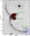 |
Fig. 1 Antennae as seen on the blue Digital Sky Survey, version 2. The light red and light blue boxes show the outer edges of the MUSE coverage as used in all further plots. The red contours mark arbitrary continuum levels derived from a smoothed HST ACS image in the F814W filter in the central interacting galaxy. The two galaxy nuclei can be used to relate their location in other figures in this paper. The blue contours are similarly derived from HST data in the region near the tip of the southern tidal tail, they mark mostly foreground stars and background objects. The two bright stars in this region can be used to relate the location of this field to the other figures in this paper. This region is sometimes called NGC 4038 S in the literature; here, we use the term south or southern to describe it. |
2 Data description
2.1 MUSE observations
The Antennae were observed during multiple nights in April and May 2015, and February and May 2016, with the MUSE instrument (Bacon et al. 2012, and in prep.). We employ the wide-field mode. This samples the sky at 0.′′2 and covers a field of view of about 1□′. The extended wavelength configuration (WFM-NOAO-E) was set up to attain a contiguous wavelength coverage from 4600 to 9350 Å. This mode incurs a faint and broad second-order overlap beyond ~8100 Å (see Weilbacher et al. 2015a,b) that is, however, not affecting our analysis.
The layout of the observations is indicated in Fig. 2. These maps display the relative weights used for the creation of the datacube (see below) which can be used to judge the relative depth of the data and is annotated with the MUSE field number of the pointings. Most pointings were taken with a spatial dither pattern at fixed position angle, with 1350 s per exposure. The shallow extra pointings (featuring an x in the name) were observed at two angles separated by 90°, Center02 was observed at position angles of 150, 240, and 2 × 330°. All observations in 2015 were interleaved with 200 s exposures of a blank sky field. This was skipped for the south pointings taken in 2016, since it was discovered that those fields offer enough blank sky already. Except for one pointing that was observed through moderate clouds (Center06x), all exposures were done in clear or photometric conditions. The seeing as measured by the autoguider probe of the VLT varied during the observations between about 0.′′5 and 1.′′2 but was generally in the sub-arcsec regime. A detailed timeline of the observations of the different fields is given in Table 1.
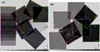 |
Fig. 2 Inverse gray-scale map of the relative weights of the data of the MUSE data of the Antennae. In this representation, the deepest regions appear black while those parts of the data only covered by exposures taken in poor conditions appear light gray. In color, boxes representing the MUSE fields (each approx. 1′× 1′ in size) are shown, with the annotated field designation and a cross marking the field center. The white contours are similar to the continuum levels shown in Fig. 1. Panel a: pointings of the central Antennae; panel b: pointings around the tip of the southern tidal tail are presented. Panel b: a removed satellite trail that decreased the effective exposure time is marked with a dashed cyan arrow. |
Layout of the observations.
2.2 Data processing
All data were consistently reduced using the public MUSE pipeline (Weilbacher et al. 2012, 2014, and in prep.)1 in v1.6.
Basic data reduction followed standard steps for MUSE data. Master calibrations were created from biases, lamp flat-fields, and arc exposures, and resulted in master biases, master flats, trace tables, and wavelength calibration tables. One set of arcs for each run was used to determine the line spread function (LSF) of each slice in the MUSE field of view. The twilight sky flats in extended mode were converted into three-dimensional corrections of the instrument illumination. These calibrations and extra illumination-flats were then applied to the on-sky exposures (standard stars, sky fields, and object exposures), using the calibration closest in time. The instrument geometry was taken from the master calibration created by the MUSE team for each corresponding run of guaranteed time observations (GTO).
We treated each extended-mode standard star exposure in the same way as Weilbacher et al. (2015a): two reductions were run, using circular flux integration and Moffat fits to extract the flux. The separate response functions were then merged at 4600 and 8300 Å, with the circular measurements for the central part of the wavelength range, equalizing the response level at the merging positions to the central part. This procedure reduces the effect of the second-order contamination in the very red and permits flux calibration even in the partially incomplete planes below 4600 Å. Next, all offset sky fields were processed, using response curve and telluric correction derived from the standard star closest in time. This produced an adapted list of sky line strengths and a sky continuum. If these sky properties needed to be applied to a science exposure taken in between two sky fields, both tables were averaged. For both sky and science fields, we used a modified initial sky line list, where all lines below 5197 Å were removed. This reduced broad artifacts near Hβ and in other regions in the blue spectral range where very faint OH bands, but no strong telluric emission lines, were present.
The science post-processing then used the closest-in-time or averaged sky properties, the LSF of the run, the response and telluric correction, as well as the astrometric solution that matches the geometry table for the respective run. To help the pipeline with the creation of an optimal sky spectrum, we used the approximate sky fraction as processing parameter. This was 10% for the central fields where the sky spectrum of the science exposure was simply used to adapt the sky line strengths, and 50% for the southern fields where at least half the field consisted of sky and hence both line adaptation and continuum computation were done using the science field itself. One exposure of the field South01 was affected by a satellite trail (visible as a lighter linear feature in Fig. 2b and indicated with an arrow); it was removed by masking the data within ± 5.5 pixels from the center of the trail.
To be able to combine all exposures, the spatial shifts of all individual MUSE cubes were computed against a corresponding HST exposure. For this, the MUSE data were integrated using the filter-function of the HST ACS F814W filter to create an image. The HST image was smoothed to approximately 0.′′6 full width at half maximum (FWHM). The centroid of the brightest compact object in each MUSE field was then measured in sky coordinates using IRAF IMEXAM and compared to the HST ACS F814W images (HST proposal ID 10188, Whitmore et al. 2010) to derive the effective offset. These were given to the pipeline for the final combination of all exposures. The positions of the few bright foreground stars in our final cube agree with positions given in the 2MASS catalog (Skrutskie et al. 2006) to better than 1.′′0 and to the positions in the Gaia DR1 (Gaia Collaboration 2016) catalog to within 0.′′3. As a result, our data have a good relative and absolute astrometric accuracy. The wavelengths of all exposures were shifted to the solar system barycenter.
We created separate cubes for the central and southern regions, each encompassing all relevant exposures. To optimize the spatial resolution of the cubes, we applied FWHM-based weighting offered by the pipeline. This uses the average seeing measured by the VLT autoguiding system during the exposure to create a weight inversely proportional to the FWHM of an exposure (similar to the procedure of Heidt et al. 2003). For the extra exposures (Center06x and Center07x) we reset the seeing in the FITS headers so that these were weighted approximately five times less than the other exposures. This ensures that these exposures only contribute significantly where other betterdata are absent. The short exposures (Center08s) were taken to cover part of the field where Hα was saturated; they contribute significantly only in the regions around the saturation, which were masked by hand in the longer exposures. We used the standard (linear) sampling of 0.′′2 × 0.′′2 × 1.25 Å voxel−1 but also created cubes in log-sampled wavelengths in the same spatial grid, where the sampling ranged from 0.82 Å pixel−1 in the blue to 1.72 Å pixel−1 at the red end; this corresponds to a velocity scale of 53.5070 km pixel−1. The pipeline also created weight cubes to show the relative contribution at each position. The wavelength-averaged version of these for the linear sampling is displayed in Fig. 2.
The effective seeing in the final cube is difficult to assess since many of the compact objects were not point sources and spatial variations remain. From the few foreground stars, we estimate a seeing at a wavelength of 7000 Å and find 0.′′59± 0.′′05 in the main central part (covered by Center01 to Center05), 0.′′76 ± 0.′′15 over the full central field, and 0.′′57 ± 0.′′07 in the southern field.
3 Structure of the ionized gas
We created initial, simple continuum-subtracted Hα flux maps from the original cubes employing two methods: (1) We summed the flux in the cubes between 6595 and 6604 Å and subtracted the continuum flux averaged over the two wavelength ranges 6552–6560 and 6641–6649 Å. These ranges were tailored to integrate as much flux as possible of the Hα line at the velocity of the Antennae without being influenced by the [N II] lines. This approach is similar to using very narrow filters matched to the redshift of the Antennae. (2) We ran a single-Gaussian fit over the whole field in the spectral region around Hα. As a first-guess for the Gaussian profiles we used the systemic velocity of 1705 km s−1 (as listed in NED2 with reference to the HIPASS survey) and the approximate instrumental FWHM of 2.5 Å; the fits used the propagated variance in the datacube. The latter approach has the advantage of integrating most of the flux of the Hα line for all spatial positions, independent of the actual gas velocity. However, it tends to overestimate the flux in regions of very low S/N. The narrow-band approach on the other hand integrates the Hα flux even in places where the emission line has broad wings or multiple components; it is also insensitive to the correlated noise in the MUSE datacubes that causes artifacts in some parts of the field. We present the results of the narrow-band technique in Fig. 3, while the Gaussian fit result for the central field is shown in Fig. 4. When accounting for the relative characteristics, the features visible in both types of maps are the same.
The line detection sensitivity of these simple approaches can be estimated using the noise near Hα. We did thatby measuring the standard deviation across two empty spectral regions of 6400–6570 Å and 6630–6705 Å. The resulting noise is overestimated in places where significant continuum exists (and hence contains stellar absorption), and it shows a pattern of correlated noise in several regions (which is normal in MUSE data), especially where single pointings or dither without rotation dominate the signal. The typical 1σ noise level in regions with four overlapping exposures is 3 × 10⁻²⁰ erg s−1 cm−2 spaxel−1 (variations from 2.4 to 3.6), equivalent to about 7.5 × 10⁻¹⁹ erg s−1 cm−2 arcsec−2. In regions with low-quality data or shorter, single exposures, the noise can reach 1.6 × 10⁻¹⁸ erg s−1 cm−2 arcsec−2. This can be compared to the 1σ limit of 4–5 × 10⁻¹⁸ erg s−1 cm−2 arcsec−2 of Lee et al. (2016, their Sect. 4), one of the deepest Hα studies of nearby galaxies to date, using a tunable filter adapted to each object. Even in the worst case, the MUSE data are still at least 2.5× more sensitive to Hα emission than the data of Lee et al., and 5× on average.
The resulting flux maps (Fig. 3) show strong Hα emission in the disks of the merging galaxies. This is highlighted in panel (a) by the light gray contours and corresponds to the well-known structures detected in previous narrow-band (Whitmore et al. 1999; Mengel et al. 2005) and Fabry–Perot (Amram et al. 1992; Zaragoza-Cardiel et al. 2014) observations of the Antennae. However, in the much deeper MUSE data, we also detect faint Hα emission around the central merger, out to the edge of the field covered by the MUSE data. This warm gas is easily visible by eye in the Hα flux map in panel (a) of Fig. 3, beyond the outermost contour. Simply summing up the detected flux in the complete Hα flux map and within the 5 × 10⁻¹⁶ erg s−1 cm−2 arcsec−2 contour – this corresponds approximately to the sensitivity limit of the Fabry-Perot data of Zaragoza-Cardiel et al. (2014) – suggests that up to 14% of the Hα flux of the central Antennae that forms the faint diffuse component has not been detected in previous studies.
The central Hα map shows several noteworthy characteristics in the faint component. Everywhere around the Hα emission of high surface brightness (beyond the 2.5 × 10⁻¹⁶ erg s−1 cm−2 arcsec−2 contour), one can see filaments reminiscent of ionized structures visible in edge-on galaxies (e.g., Rossa et al. 2004) and starbursts with outflows (Heckman et al. 1995; Lehnert & Heckman 1996). Such structures are frequently attributed to starburst events in the centers that through stellar winds and supernova explosions give rise to superbubbles and chimneys (Ferguson et al. 1996; Rossa & Dettmar 2003) and might provide pathways of low density to allow Lyman-continuum photons to travel into the surroundings (Lee et al. 2016, e.g., in UGC 5456). Further away, filaments in north-south direction dominate the MUSE data. These are oriented in the same way as the ridgeline3 of the (southern) tidal tail. These could be related to the stretching of the material by the tidal forces that form both tidal tails. A string of bright HII regions can be seen in the same regions. In the outskirts, away from the edge of the tidal tail, east–west filaments can be seen as well. A hint of another such feature is marginally visible in the data to the west of the merger.
In the targeted region near the end of the southern tidal tail, several HII regions are apparent (Fig. 3b). Some of the brighter ones are surrounded by diffuse emission, but unlike the central region there are large spatial gaps between the multiple Hα detections. FilamentaryHα of the same type as around the central region is not visible anywhere in this field. The regions detected already by Mirabel et al. (1992, denoted I, II, and III) can be associated with some of the brightest regions detected in the MUSE data. We show the positions as recovered by Hibbard et al. (2001)4 in Fig. 3b. If Fig. 1b of Mirabel et al. and Fig. 6 of Hibbard et al. are correct, then the slit of those observations was located just in between close pairs of HII regions. Their 1.′′5 slit was probably wide enough to integrate light from both components of each region. However, with that single slit, they missed the brightest regions, and with EFOSC on the ESO 3.6m telescope they were not able to detect any of the fainter regions. Of the compact Hα detections in the comparatively shallow Fabry-Perot data of Bournaud et al. (2004, their Table A.1 and Fig. A.8) only three (3, 4, and 6) can be matched to something in our data, after correcting their positions by an offset of 2.′′9. Two other detections (1 and 8) are outside the field of our data, three more (2, 5, and 7) are not present in our data, suggesting that they were spurious sources. None of the other similarly bright HII regions (such as the Mirabel sources II and III) were picked up in the FP data. The velocities measured by Bournaud et al. are higher than the estimate using our Gaussian fit by ~180 km s−1 (objects 3 and 4) and ~160 km s−1 (object 6), far outside the 1σ = 3…5 km s−1 measurement error of those bright regions in our data.
In the following two sections we characterize the diffuse emission and the HII regions.
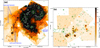 |
Fig. 3 Continuum-subtracted Hα flux maps for the central (panel a) and the southern (panel b) region, as produced by the narrow-band technique (see text). The common color scaling (color bar on the right) was chosen to highlight faint features. The black-to-gray contours denote the Hα flux levels, smoothed by a 3-pixel Gaussian, of 2.50 × 10⁻¹⁷, 1.25 × 10⁻¹⁶, 2.50 × 10⁻¹⁶, 1.25 × 10⁻¹⁵, 2.50 × 10⁻¹⁵, and 1.25 × 10⁻¹⁴ erg s−1 cm−2 arcsec−2; since the emission in the southern region is fainter, not all contours are visible in panel b. The green contours highlight continuum features and are identical to those shown in Fig. 1. In panel b, the blue circles and corresponding roman numerals denote the detections by Mirabel et al. (1992) with coordinates from Hibbard et al. (2001), while the red circles and arabic numerals are detections by Bournaud et al. (2004). |
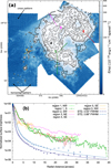 |
Fig. 4 Radial profiles of the Hα surface brightness compared to the point spread function (PSF) as derived from two typical standard star observations. Panel a: Hα flux map from Gaussian line fits to the emission line, comparable to Fig. 3a, but with radial extraction cuts marked and the corresponding Hα peaks numbered. Low-level patterns caused by the correlated noise in the MUSE cubes are marked with arrows. Panel b: radial flux distribution outwards from the HII regions. The markers in the map and the corresponding profiles are shown with the same color. The PSFs derived from the standard stars are shown as elliptical profiles with error bars and triple Moffat fits. |
4 Diffuse ionized gas
4.1 Verification of the visual appearance
To verify that the visual appearance in Fig. 3a is correct and that the diffuse outer Hα detection is not caused by the instrumental plus atmospheric point spread function (PSF, see discussion by Sandin 2014, 2015), we compared the extended emission to the PSF in two different ways, using a radial extraction of the data and by convolving the high surface-brightness data with the PSF.
Since the stars in the Antennae MUSE data are too faint to construct a PSF over more than a 1–2″ radius, we used two typical standard stars (LTT 3218, observed on 2015-05-21 in 0.′′88 seeing at ~6600 Å, and LTT 7987, of 2015-05-13, 0.′′53 FWHM) observed in the same mode as the Antennae data. These stars are bright and isolated enough to construct a PSF, using ellipse fitting, out to a radius of at least 30″. Both stars were observed in a four-position dither pattern, reduced as a science frame with the MUSE pipeline, and each combined into a deeper cube. The PSF was then determined on a two-dimensional (2D) image averaged from the wavelength range 6570–6634 Å, using the ELLIPSE task running in the IRAF/STSDAS environment, and subsequently also fitted with a triple Moffat function. As comparison, we extracted radial profiles, from the peak of a few of the brightest Hα peaks toward surface brightness minima of the Hα map. The radial cuts and the resulting radial profiles are shown in Fig. 4. The PSF as measured from the standard stars is well constrained out to about 20″ radius, that is, over 5 orders of magnitude. Beyond 25″ the variations are significant, since the standardstars are not bright enough5. The extracted Hα profiles in this normalized view are consistently above the PSF, up to 2 dex higher at 5″ , 1.5 dex at ~15″, and still 1 dex higher than the mean PSF at radii approaching 30″ and beyond. This and the presence of small-scale structure indicates that scattered light has only minor contributions to the extended emission.
As an alternative, we tested the Hα maps that would result when convolving the bright parts of the Hα emission with a MUSE PSF. We therefore set all pixels in the Hα map with a flux below 2.5 × 10⁻¹⁶ erg s−1 cm−2 arcsec−2 to zero and convolved the resulting image with both PSFs. Unsurprisingly, the resulting images show a smooth outer appearance, and no structure in the outskirts of the type that is visible in Fig. 3a. After subtracting the convolved images from the original Hα map, the features and especially the filamentary structure in the outskirts are even more enhanced. Tests with different cut-off levels (6.25 × 10⁻¹⁶ and 2.5 × 10⁻¹⁵ erg s−1 cm−2 arcsec−2) show that it is not possible to explain the observed faint features as wings of high-surface-brightness emission and a typical MUSE PSF.
Finally,we looked at the velocities measured from the Hα line. To derive them, we employed the p3d environment (Sandin et al. 2010, 2012) to fit a single Gaussian profile to the Hα line6 . We used the continuum-free cube (Appendix A.1) binned to a Hα-S/N of 30 as input. The resulting Hα velocity map is shown in Fig. 5. This map clearly shows variations of the measured velocity, also in the outskirts where the faint Hα filaments are detected. If they were due to scattered light, they would show a smooth distribution of velocity in radial direction.
We conclude that the faint filamentary structures seen in the Hα emission line are a real feature of the outskirts of the central Antennae field, and that scattered light only plays a secondary role.
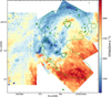 |
Fig. 5 Velocity derived from the Hα emission line in the central field of the Antennae. The velocities are corrected to the solar-system barycenter and are computed over bins of S∕N ~ 30 (see text). The green lines are the same HST broad-band contours as in Fig. 1. |
4.2 Properties of the diffuse ionized gas
Even at thedepth of the MUSE spectroscopy, the diffuse ionized gas (DIG) is too faint for us to derive physical properties with good spatial resolution. We therefore start measuring spectra of large integrated regions in the central merger. We divide the data into three surface brightness levels: bright (H α≥ 10−16 erg s−1 cm−2 spaxel−1), intermediate (10−17 ≤Hα < 10−16 erg s−1 cm−2 spaxel−1), and faint (H α< 10−17 erg s−1 cm−2 spaxel−1). To integratethe spectra we exclude the regions determined to be HII regions in Sect. 5. We then follow the pPXF analysis (Appendices A and A.2) to measure the average emission line fluxes over these regions. We correct for extinction using the Balmer decrement, and compute electron densities (using the [S II]6716.31 line ratio) and temperatures (from the [N II]6548,84 to [N II]5755 ratio), using PyNeb (version 1.0.26; Luridiana et al. 2015). The results are shown in Table 2. The errors quoted there are 68% confidence limits, computed using 100 Monte-Carlo iterations, using the flux measurement errors propagated from the lines involved in the cross-iteration of both quantities. The values indicate very low extinction, and subsequently lower densities and higher temperatures as we go to fainter Hα surface brightness. However, for all three diffuse spectra, the [S II] diagnostic ratio is close to the low-density limit.
Using these measurements, we can also position the faint Hα emitting gasin diagnostic diagrams, as presented in Fig. 6. For reference, we show the extreme photoionization line of Kewley et al. (2001), even though the mechanism in the DIG may be different. Except for the faintest level, the data lies within the Kewley et al. limit, for all three diagnostics.
It is well known that DIG often shows [S II]/Hα and [O I]/Hα ratios in regions of the diagnostic diagrams that usually indicate other types of ionization besides photoionization (e.g., Haffner et al. 2009; Kreckel et al. 2016). Several explanations for this are discussed in the literature. Shocks are an obvious candidate, but they cannot always explain all observed properties (see e.g., Fensch et al. 2016) at the same time. Zhang et al. (2017) find evolved stars to be the most likely candidate source of the ionizing photons. Hoopes & Walterbos (2003) and Voges & Walterbos (2006) suggest that this can be caused by ionization of the DIG by leaking HII regions where the UV spectrum is hardened bythe absorption inside the ionized nebulae. This then shifts the line ratio diagnostics beyond the usual photoionization limit.
In the case of the Antennae, the latter suggestion seems to fit the properties discussed here as well. Shocks have been reported in the Antennae (e.g., Campbell & Willner 1989) but they seem to be related to starburst activity in the denser regions (Haas et al. 2005). The low density of the gas in the outskirts, free of any density gradients at our spatial resolution as determined by the [S II]6716.31 line ratio, makes it unlikely for the high [O I]/Hα and [S II]/Hα ratios there to be caused by shocks. Our three-zone measurements suggest that the ionizing spectrum is still close to that of hot stars immediately surrounding the HII regions (the bright regions). Only in the faint regions, furthest away from the H II regions, are the line ratios beyond being photoionized, suggesting that the ionizing spectrum is harder there. This fits well with the models of Hoopes & Walterbos (2003), if we assume that to reach the gas to be ionized, the UV photons have to travel through even higher column densities of gas, resulting in even harder UV spectra7 . Although most studies focus on the young stellar populations in the Antennae, old stars with ages >10 Gyr exist in the disks of both interacting galaxies (Kassin et al. 2003). It may well be, therefore, that evolved stars contribute to the ionization ofthe DIG, however, as Zhang et al. (2017) point out, they are unlikely to be the dominating source in starburst galaxies. Wewill revisit the contribution of old stars in a future publication about the properties of the stellar populations. In the present paper, we focus on whether or not we can actually find evidence for Lyman-continuum leakage from the star-forming regions (see Sect. 5.5).
In Fig. 7a, we show [N II]6548.84/Hα, the line ratio with the highest S/N, in a spatially resolved manner. This map was computed using single Gaussians fit to Hα and both [N II] lines, using the p3d line-fitting tool, on the continuum-free cube discussed in Appendix A.1, after binning this cube to S∕N ≈ 30 in the Hα emission line. The faint ionized gas does not have uniform line ratios at given surface-brightness levels, but an overall trend is visible: an increase of [N II] with regard to Hα for fainter surface-brightness levels of the gas. The most striking features of this map can be seen in the eastern part, that is, the region of the tidal tail: along the ridge of the tail and around the HII regions detected there, the [N II] line is relatively weak ([N II]/Hα ≲ 0.8 or log10([N II]∕Hα) ≲−0.08). Next to this ridgeline, however, we see strongly increased [N II] emission ([N II]/Hα reaches values above 1.25, or log10([N II]∕Hα) ≳ 0.09). In the same way, at the south-western edge of the field, in the outer disk of NGC 4039, we also see a strong increase of [N II] with respect to Hα. These features are visible in a similar way in the map of [S II]6716.31/Hα which we show in Fig. 7b. To the east, around a declination of −18°52.′5, we see a broad, somewhat triangular region with weak [N II] (marked in Fig. 7a with a blue arrow), which lies slightly south of one of theeast–west filaments marked in Fig. 3a. This region coincides with a region of higher velocity gas as measured from the Hα line (Fig. 5) but is not remarkable in any way in the [S II]/Hα map. A similar region lies near the border of our field at the western edge, around a declination of −18°52.′7 (pointed to by the pale green arrow). Here, the velocity field suggests the presence of lower-velocity gas with regard to surrounding regions. Both regions counter the general trend of stronger [N II] emission in fainter gas. Given the velocity difference, it is tempting to think of these as outflows from more central regions. Since the Antennae do not contain AGN (Brandl et al. 2009) and no bright ionizing source is located near the eastern region, the source of such outflows remains unclear. The western [N II]-strong region lies close to the strong star-formation sites in the western spiral arm of NGC 4038 (regions R, S, and T; see Rubin et al. 1970) of which region S was as already found by Gilbert & Graham (2007) to be the source of an (local) outflow from line-width measurements of the Brγ line.
Properties of the diffuse ionized gas.
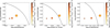 |
Fig. 6 Diagnostic diagrams showing the properties of the faint ionized gas. The radius of the three data points in each panel scales linearly to the square-root of the area, and the error bars aresmaller than the size of the points. The color is coded according to the average Hα surface brightness. The solid line indicates the nominal photoionization limit of Kewley et al. (2001). |
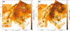 |
Fig. 7 Flux ratio maps; [N II]6548.84/Hα (panel a), [S II]6716.31/Hα (panel b). Both are Voronoi-binned to S∕NHα ~ 30. Overplotted are the same Hα contours as in Fig. 3a and broad-band levels as in Fig. 1. Features discussed in the text are marked with arrows. |
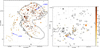 |
Fig. 8 H II regions detected in the Antennae using the ASTRODENDRO package. The common color-scale gives the Hα flux of each region. Left panel: central region; right panel: southern region. The contours are the same broad-band levels as in Fig. 1. H II regions whose spectra are displayed in Fig. 9 are marked. |
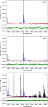 |
Fig. 9 Three example spectra of H II regions: c1665 is located near the NGC4038 nucleus, c349 is in the tidal tail of the central field, s9 is in the southern field. The corresponding regions are annotated in Fig. 8. In each upper panel, the black line shows the extracted data, the red line is the continuum fit and the blue lines represent the fit to gas emission. The green points with error bars in the lower panels show the residuals of the pPXF fit. |
5 The H II regions
To probe the possible origin of the diffuse ionized gas, we turn to the HII regions. Some of them are already directly visible in Fig. 3.
5.1 Spectral extraction
We extract peaks in the Hα flux maps using the dendrograms tool8. This tool detects local maxima and extracts them down to surface-brightness levels where the corresponding contours join. This is repeated in a hierarchical manner until a global lower limit is reached. The resulting tree structure can be used to track hierarchical relations between the individual detections. Here we only use the leaves of the structure, that is, the individual local peaks, which we take as defining the size of the HII regions to extract. Since contours at surface brightness levels below the limits of theleaves already encompass multiple peaks, other structures created by the dendrogram are ignored here.
As input to compute the dendrograms, we use continuum-subtracted Hα images computed directly from the MUSE cubes; see Sect. 3. To prevent the algorithm from identifying too many noise peaks, we process regions where only a single or poor-quality exposure dominated the data – these are the light-gray regions visible in Fig. 2 – with a spatial 3 × 3 median filter. We then filter the whole extent of the images with a 2D Gaussian of 0.′′6 FWHM to enhance compact sources, and configure astrodendro to find local maxima down to a level of 2.625 × 10⁻¹⁹ erg s−1 cm−2 spaxel−1 and require that all HII regions have at least seven spatially connected pixels. These parameters result in 42 901 dendrogram elements in the central field and 1501 in the southern field. From these, H II regionsare selected as those leaves which have a peak level over the background of at least 2.625 × 10⁻¹⁹ erg s−1 cm−2 spaxel−1. All parameters were found by trial and error, visually checking that both real peaks in the bright central region and faint ones in the outskirts were detected, but no diffuse regions or noise peaks. The resulting list comprises 556 for the central field and 63 for the southern region. The mask of each leaf is used to extract an average spectrum and associated variance from the original MUSE cubes.
5.2 Spectral analysis
To analyze the spectrum of each region, we use pPXF, with the setup described in Appendices A and A.2. This gives us emission line fluxes and error estimates. Through the stellar population fit, the Balmer lines were corrected for underlying absorption, with typical EW(Hα) in the range 1.7–2.7 Å. The data for all emission lines are dereddened for further analysis using the Balmer decrement of 2.86 and the parametrization of the starburst attenuation curve of Calzetti et al. (2000). We again compute this using the PyNeb tool. Regions with lower Balmer line ratios are not corrected, spectra with Hα/Hβ < 2 are discarded (5 and 8 for the central and southern regions, respectively); most of them are spectra with low S/N or dominated by foreground stars9 where the emission line fit does not work well.
The final sample of HII regions therefore consists of 551 in the central and 55 in the southern field. In Fig. 9, we present three typical spectra for the HII regions that we detect and analyze using the MUSE data; they are also annotated in Fig. 8. Of these, c1665 is one of the few regions, which show enough continuum features to give a reliable continuum fit. The region s9 is a fainter HII region where the sky line residuals become apparent in the spectrum. However, the lines relevant to this study are located in spectral regions without bright telluric emission lines, and hence the measurements are unaffected by these artifacts.
5.3 Basic properties of the HII regions
The first result of this procedure is displayed in Fig. 8, where the actual pixels of each extracted HII region are color-coded with the total Hα flux of each region before extinction correction. It is apparent that the brighter HII regions are located preferentially in the central part of the merger, and reach up to f(H α) = 4.9 × 10⁻¹³ erg s−1 cm−2, while the outskirts of the interacting center and the region in the southern tail show only fainter regions, up to f(H α) = 2.7 × 10⁻¹⁵ erg s−1 cm−2.
We show the Hα luminosity function (LF) of the detected regions in Fig. 10, for the central and southern fields. To derive the luminosity, we used the reddening-corrected fluxes, computed using the Balmer decrement, and assumed a distance of 22 Mpc (Schweizer et al. 2008). For comparison, we plot the LF derived from the table of HII regions based on GHαFaS Fabry-Perot observations, publicly released by Zaragoza-Cardiel et al. (2014) who used the same distance. It is apparent that we detect more regions in the luminosity range log10L(Hα) = 36…39 whereas the GHαFaS data show regions with log10L(Hα) > 39.5. Their most luminous regions are also detected in our data, but their flux determination is higher by up to one order of magnitude, owing to the extinction correction (J. Zaragoza Cardiel, priv. comm.). For the same regions we infer only moderate reddening from the Balmer decrement. Since our measurements are based on individual Balmer lines instead of correction through narrow-band filters – where the fluxes can be affected by neighboring emission lines and the relative absorption under each line can lead to an overestimate of the extinction10 – we believe that our estimates are more realistic. The difference in the medium to low luminosity range can be explained by the difference inatmospheric seeing (Pleuss et al. 2000; Scoville et al. 2001); in worse seeing conditions, more regions blend with each other and hence form fewer, brighter apparent regions, while more fainter regions remain undetected. Since the seeing in the GHαFaS data was ~0.′′9 while our effective seeing is around 0.′′6 this difference is not unexpected. We also have deeper data and can detect fainter regions, in the range below log 10L(Hα) ≲ 36.5. A more definitive HII region-LF for the bright end would require a wide-field IFS with HST-like spatial resolution. We also note that ongoing work on MUSE data from the nearby galaxy NGC 300 (distance 1.87 Mpc) is revealing even fainter compact H II regions (Roth et al. in prep.), below the detection threshold of our Antennae data.
We see again that the LF in the southern tidal tail is devoid of bright HII regions. While the most luminous region in the central part reaches  erg s−1, in the southern part we find only
  erg s−1. To investigate if this is just an effect of the different sizes of the two samples, we randomly drew one million samples of 55 H II regions from the 551 regions in the central merger. All of these samples contained at least three regions with
  erg s−1. Despite the small number of detections in the southern region, we also notice that the slope of both LFs is different: while we detect a similar number of regions in the histogram bin of
  , the central histogram shows a strong increase up to a turnover at
  . The numbers in the southern bins on the other hand decrease almost monotonically to the maximum lumonosity of
  , without any turnover. Using the same random sampling we find that the numbers of HII regions in the southern field in the luminosity bins at 36.125, 36.375, and 36.625 are 11.3σ, 5.7σ, and 6.3σ outside the expected range, if drawn from the same population as the HII regions in the central field. We conclude that the H II region samples in the central and the southern fields are of intrinsically different luminosity distribution.
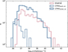 |
Fig. 10 Hα luminosity function for the HII regions detected in the Antennae using the astrodendro package. The bold blue lines (solid: central region, dashed: southern field) show the luminosity histogram in our MUSE data of the Antennae, after correction for internal extinction. The red solid line shows the luminosity function of Zaragoza-Cardiel et al. (2014). |
5.4 Diffuse gas fraction
We can now compare the Hα flux measured in the HII regions with the flux elsewhere to derive the fraction of the diffuse ionized gas in the Antennae. The flux of all H II regions is the sum of the flux inside the masks of the dendrogram leaves that are used as HII regions. By inverting the mask, we derive the flux of the diffuse gas.
In the simplest and most consistent way, we apply both masks on the narrow-band continuum-subtracted image of both fields as created at the beginning of this investigation (Sect. 3). This yields the fluxes presented in the “masking” row of Table 3 from which we derive the most direct estimate of the diffuse gas fraction of ~60% for the central merger and ~10% for the southern field11.
For the central field, we can derive the integrated flux using alternative approaches, using the spectra that we analyzed as detailed in Sects. 5.2 and 4.2. Summing the flux over all extracted spectra – once for all H II region measurements, and once for the three integrated spectra of the DIG, both before extinction correction – gives the value in the “spectral” row. This gives a comparable value for the central field, with about 60% DIG fraction.
To relate that to the amount of Lyman-continuum photons available in the HII regions, we also look at the Hα flux after extinction correction. Those measurements are given in table row speccor. Since the extinction in parts of the central merger is known to be high (e.g., Mengel et al. 2005; Whitmore et al. 2010) – a property that we can confirm with our measurements – this strongly affects the estimate of the total Hα flux. The corrected HII region flux is twice as high as without the correction. On the other hand, the extinction in the diffuse gas is very low, so the integrated flux in the DIG remains comparable. This results in a significantly lower speccor estimate of fDIG ≈ 45%.
Since the HII region measurements are affected by the underlying diffuse component (see e.g., Kreckel et al. 2016), we also performed a check using a spectral extraction routine that aims at subtracting the surrounding background around each region. For this, mask dilation is used to define a gap of approximately 2 pixels and then a background annulus with a width of about 3 pixels. This results in background regions that typically have the same sizes as the areas of the HII regions. To minimize the influence of other nearby Hα peaks, we subtract the median spectrum over this background annulus. However, for many regions this subtraction does not work very well, meaning that the resulting spectral properties vary in unphysical ways. We therefore only use this spectral extraction as a cross-check, for the sample as a whole. The integrated HII region flux estimated from this extraction is given in table row specsub. It is about 30% smaller than the spectral estimate. We then add this difference to the spectral DIG estimate and assume that the total Hα flux has not changed. This results in a moderate change to a fDIG ~ 70%.
For the southern region, the spectral estimates cannot be done in the same way. Integrating the data over everything outside the H II regions cannot work, since most of the data is filled either with residual noise, background galaxies, or foreground stars. Such a procedure would therefore need extensive manual editing of a spatial mask and rely on the information from the masking approach. To nevertheless give similar estimates for the DIG fraction, we correct the total flux by the difference in HII region flux, and re-use the DIG flux from the masking technique. For the southern field, we then estimate a spectral DIG fraction of about 13%. Since the extinction is very low in most HII regions in that field, the speccor fraction is very similar, roughly 12%. Both approximately agree with the basic masking estimate. For specsub we assign the Hα flux that the HII regions lost by subtracting the surrounding flux to the DIG which then results in a significantly higher fDIG ~ 27%.
To summarize, the fraction of diffuse Hα emission in the Antennae is about 60% for our central field and about 10% for the southern region. After trying to correct for diffuse emission underlying the HII regions, we estimate even higher DIG fractions of 70% and 27% for the central and southern fields, respectively.
Integrated Hα fluxes in the different components (in units of erg s−1 cm−2).
5.5 Search for leaking HII regions
As the observations of Hibbard et al. (2001) have shown, there is about 5× 10⁹ M⊙ in atomic hydrogen available in the Antennae, which would be ionized if a sufficient number of Lyman continuum (LyC) photons escaped from the star-forming regions and young star clusters. Indeed, Hibbard et al. suggested exactly this as explanation for the gap at the base of the northern tidal tail that is visible in the H I data, but not covered by the MUSE data. Using our sample of H II regions we therefore want to check the fraction of the diffuse gas that is detected in our data that could be due to leaking LyC photons from those star-forming regions.
We have estimated that after correction for extinction, 45% of the Hα flux is detected as diffuse gas in the central field and 12% in the southern field. These values should not be compared to LyC escape fractions of galaxies, which are typically estimated to be on the order of a few percent (Leitet et al. 2013; Leitherer et al. 2016). Instead, we need enough photons escaping from the HII regions into the surrounding medium that is still bound to the interacting galaxies and strongest in the high-surface brightness parts of the object, that is, close to the star-forming regions themselves. Further, for HII regions in nearby galaxies, several studies have found significant LyC escape fractions of 50% and more for some of the most luminous regions (Voges et al. 2008; Pellegrini et al. 2012). Whether the galaxy as a whole is then a LyC leaking object depends on the fraction of LyC radiation consumed to ionize the interstellar gas.
Our spectral fits using pPXF do not constrain the LyC flux. These fits were only created to approximate the absorption below the Balmer lines and hence take out the continuum slope using polynomials (see Appendix A). We postpone a full assessment of the stellar population using the MUSE data to a future publication. Instead, we compare to the analysis of the young star clusters by Whitmore et al. (2010) who used broad and medium-band HST data to estimate masses and ages of all compact sources that were detected with high-enough S/N. This analysis is based on several colors and does not rely on the identification of the spectral type of single stars as in the NGC 300 work of Niederhofer et al. (2016), who find that when assessing the stellar sources inside HII regions using only stellar broad-band data, constraining the escape fraction has a high degree of uncertainty. The Whitmore et al. analysis fits stellar populations to the multi-band (U to I and Hα) cluster data. The broad-band filter selection agrees with the recommendations of Anders et al. (2004) and Fouesneau & Lançon (2010) for the analysis of young clusters and provides a solid base for the analysis. Since the estimated masses of the young clusters with the strongest LyC flux are above 104 M⊙, and often beyond 106 M⊙, the initial mass function should be well-sampled, making the estimate of Q(H0) relatively insensitive to effects of stochasticity (Anders et al. 2013). Additionally, their use of the F658N filter effectively breaks the age-extinction degeneracy (see Fouesneau et al. 2012) and assigns realistic ages, especially for young ages <10 Myr which are important for our analysis. However, since it is a priori unclear which parts of the H II regionsare ionized by a given cluster and Whitmore et al. only integrated the fraction of Hα flux within the cluster aperture, the F658N filter cannot strictly help to distinguish between different young ages, as long as Hα emission is present. Another issue is that no UV data shortward of the F336W filter exists with sufficient spatial resolution over the full field; this would otherwise have better constrained the continuum slope and hence the age of the youngest population. The contribution of emission lines to broad-band filters is another source of uncertainty (Anders & Fritze-v. Alvensleben 2003); these emission lines might mask the appearance of the 4000 Å break in populations older than a few Myr and cause the mass to be overestimated. Fouesneau et al. (2012) thoroughly investigated the systematics involved in the determination of cluster populations from U, B, V , I, Hα filters, and found a standard deviation of 0.14 dex for the age determination. They also note that clusters with ages younger than ~5 Myr tend to be assigned older ages. Chandar et al. (2016), who used the same analysis technique and filter set as Whitmore et al. (2010), estimated the 1σ error bar on the age and mass estimates to be 0.3 dex. Since the LyC flux of a stellar population evolves nonlinearly, the ~0.2 dex uncertainty in age can be translated into uncertainties in the LyC rate between 1% and one order of magnitude (depending on the actual age estimate), but may be underestimated for individual star clusters. Despite the fact that the uncertainties are significant, we assume that masses and ages of the clusters as presented by Whitmore et al. are robust enough for our purpose – the assessment of LyC photon flux.
From the Whitmore catalog12 we first select all clusters with valid measurements in at least the F336W, F435W, and F814W filters. From these we further select those for which a valid mass estimate exists and where the logarithmic age estimate is between 6.0 and 7.8. These clusters should be responsible for the total LyC flux ionizing the HII regions in the Antennae. From the total catalog, 2162 clusters meet these criteria. We then match the position of the clusters to the extent of each HII region on the sky. We compute the LyC flux Q(H0) expected from each cluster by comparison to a solar-metallicity13 GALEV model (Kotulla et al. 2009), computed using the Geneva isochrones. To be consistent with the Whitmore et al. population analysis and the origin of the LyC-to-Hα conversion factor given by Kennicutt (1998) we used a Salpeter (1955) initial mass function with a mass range 0.1–100 M⊙. Then we compare the rate of LyC photons produced by the population of young clusters inside the region with the rate of ionizing photons computed from the Hα luminosity, using the conversion factor Q(H0) = 7.31 × 10¹¹L(Hα) (Kennicutt 1998), resulting in a LyC escape fraction fesc for each H II region.
Since the GALEV code uses the table of Schaerer & de Koter (1997) to compute the Lyman-continuum flux, which was shown to overestimate the UV flux in some early phases of young stellar evolution (Smith et al. 2002), we also cross-checked the results using Starburst99 (v7.0.1; Leitherer et al. 1999, 2010; Levesque et al. 2012) which implements a more modern treatment of the UV spectrum and also makes use of newer Geneva isochrones. In order to run Starburst99, we otherwise use inputs comparable to the GALEV models, especially using the fixed-mass instantaneous star-formation history.
The results are as follows: from comparison with the GALEV model, of the 551 HII regions, 108 leak LyC photons at a rate of Q(H0) = 2.7 × 1053 s−1 while 112 regions are optically thick to UV radiation. The results are presented in Fig. 11. Most of the HII regions with non-zero escape fraction are located in the inner parts of the merger, for example, in the overlap region and in the center of NGC 4038, the northern nucleus. But there are also a few regions in its outskirts, especially near the northern edge of our field of view, in the outer disk of NGC 4038. We note that there are 331 for which we cannot identify an ionizing source in the form of a young cluster in the sample of Whitmore et al. (2010) that spatially coincides. These were assigned a light gray color for the presentation in Fig. 11. As marked in this figure, 14 of the HII regions without ionizing source are located outside the limits of the HST multi-band coverage. The others might be the result of the sensitivity limits of the HST observations, possibly in conjunction with different extinction towards the region of line emission and the stellar location (see e.g., Heydari-Malayeri et al. 1999).
If the estimates computed with SB99 are taken to be more realistic, then 127 of the 551 HII regions are partially optically thin to Lyman continuum photons and leak an even higher number of Q(H0) = 3.2 × 1053 s−1 into the surrounding medium.
Since the Hα fluxes that we used in this section to estimate the LyC escape of every HII region were computed in the apertures without correcting for the diffuse background, the numbers given above might have been affected by the same diffuse ionized gas for which we are trying to find the origin. To test this hypothesis, we turn again to the background-subtracted H II region measurements that we already used as cross-check in Sect. 5.4. With this dataset and in comparison to the GALEV estimate, we find a total of 115 optically thin nebulae which appear to leak 2.9 × 1053 s−1 LyC photons; with SB99 we again find higher numbers of 3.4 × 1053 s−1 leaked by 137 HII regions.
Another effect that might influence our estimate is the reddening by dust. If the light of some of the HII regions is not only extinguished along the line of sight, but also into other directions, the LyC photons could be absorbed before reaching the surrounding neutral medium. To model this, we assumed that the extinction within the galaxies follows the same distribution of dust screens as towards the observer. We therefore reduced the summed LyC photons inside each region by the respective UV extinction, drawn randomly from the sample of reddening values. We created 100 Monte-Carlo iterations with this method and found a distribution around an average of  s−1. However, since star formation hidden from the observer but not necessarily from the rest of the central merger is known to exist (Mirabel et al. 1998; Mengel et al. 2005), the total number of LyC photons that do not get absorbed by dust is likely higher than this estimate. Since the dust reddening for each HII region within the galaxy cannot be made with any certainty, we keep the above GALEV analysis for further discussion, with the fiducial value of Q(H0) = 2.7 × 1053 s−1.
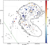 |
Fig. 11 H II regions detected in the central Antennae. Here, the color indicates the Lyman-continuum escape fraction fesc, estimated bycomparing Hα luminosity and illuminating young star cluster(s). All colored regions have a positive escape fraction, other regions are filled light gray. The contours are the same broad-band levels as in Fig. 1, and the dashed dark-green line shows the approximate limit of the HST imaging. |
5.5.1 LyC leakage and emission-line ratios
Several studies have recently used emission-line ratios composed of lines of different ionization energy to find HII regions (and whole galaxies) that are likely to leak significant amounts of ionizing photons. The ratio [O iii]/[O II] is frequently used, since it was found to be high ([O iii]/[O II] ≳ 5) in galaxies that were observed to leak LyC photons (Izotov et al. 2016a,b). Similarly, high ratios of [O iii]/[S II] (Pellegrini et al. 2012) are indicative of leakage of LyC photons.
Since MUSE is missing the blue wavelength coverage that would allow detection of the bright [O II]3727.29 doublet for such nearby galaxies, and the line ratio [O iii]/[S II] also depends on the relative abundances of oxygen and sulfur, one may prefer to use ionization-parameter-sensitive line ratios of the same elements, namely [S iii]/[S II] (Zastrow et al. 2013) and [O iii]/[O I] (Stasińska et al. 2015). In normal, ionization-bounded HII regions one expects a region of lower ionization gas on the outskirts (Osterbrock & Ferland 2005). So, if the low-ionization line exhibits unusually low flux compared to a high-ionization line in the same region, this would show a region to have an unusually thin or non-existing transition region, as one might expect in density-bounded, that is, LyC-leaking regions. However, since the size of the transition region or the ionization front depends strongly on the ionizing source (Osterbrock & Ferland 2005; Pellegrini et al. 2012), it is difficult to give an absolute limit for any of these line ratios. At a spatial resolution of about 60 pc, we lack the ability to carry out proper ionization parameter mapping (cf. Pellegrini et al. 2012) of the HII regions to find better indications of which of them is optically thin.
However, assuming that our approach with the cluster population analysis gives a good estimate of the real LyC escape fraction, we can check if there is a correlation of the line ratios with fesc . We show the results in Fig. 12, for all three line ratios that MUSE covers. We discuss these results quoting numbers based on the more conservative GALEV analysis (SB99 values differ typically by only 10%).
The plot with the [O iii]/[O I] ratio (in Fig. 12a) does not give a strong visual impression of a correlation. However, there are 12 regions with [O iii]/[O I] ratio above 30, with 10 of them showing positive LyC escape fractions of up to 90%, summing up to LyC rates of 1.3 × 1053 s−1 that are available to ionize H I outside the star-forming regions. The same picture emerges with the [S iii]/[S II] line ratio (Fig. 12b). There is again a broad range of escape fractions for low sulfur line ratios, without a strong correlation. However, of the HII regions with the highest [S iii]/[S II] ratio (>1.25), 9 of 11 are LyC leakers in accordance with the above criteria, producing 1.2 × 1053 s−1 ionizing photons. There are 8 regions that are above the given limits for both [O iii]/[O I] and [S iii]/[S II], and 7 of them are estimated to be at least partially density-bounded. For the line ratio [O iii]/[S II] as plotted in Fig. 12c, all 10 of the HII regions with [O iii]/[S II] > 2.5 appear to be optically thin, and leak 5.7 × 1052 s−1 LyC photons into their environment.
To conclude this section, we can say that the Lyman-continuum escape fraction is not directly correlated with the ionization-parameter-sensitive line ratios. Very high values of all three of the studied line ratios, above certain limits, on the other hand, are a clear sign that a HII region is density bounded, and seem to signify LyC leakage at a rate between about 20 and up to 90%.
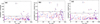 |
Fig. 12 Ionization-parameter-sensitive line ratios against Lyman-continuum escape fraction (fesc) for our sample of HII regions. Panel a: line ratio [O iii]5007/[O I]6300; panel b: [S iii]9068.9531/[S II]6716.31, and panel c: [O iii]5007//[S II]6716.31. In all plots, the blue points are the results using the GALEV model while the red points shows the escape fraction computed using SB99. 1σ ranges of the statistical error of both axes are plotted as gray lines for the GALEV results. Violet points at the left border are those regions which were found to be optically thick. Horizontal dashed lines denote lower limits of the line ratios with high escape fraction, as discussed in the text. |
5.5.2 Lyman-continuum photon budget
As we have shown above, MUSE data, in conjunction with HST cluster analysis, suggest that many HII regions in the central part of the Antennae merger are optically thin and leak LyC photons at a very high rate of Q(H0) = 2.7 × 1053 s−1, as the most conservative estimate without internal extinction.
If our computation of an Hα flux in the diffuse gas component of f(Hα, DIG) ≈ 6.02 × 10⁻¹² erg s−1 cm−2 (after extinction correction, see Sect. 5.4) is correct, a rate of 2.55 × 1053 s−1 LyC photons is needed to ionize the H I in the central Antennae. This now suggests that all photons necessary to ionize the diffuse medium can be provided by leakage from the star-forming regions.
Unfortunately, the catalog of Whitmore et al. (2010) only covers our central field; we cannot use it to run the same analysis for the southern part of the MUSE data. While some HST data exists over the MUSE pointings, the coverage is incomplete and consists of only a subset of the filters that are required to do a proper analysis of the stellar populations. Therefore, as an alternative approach, we use the 386 HII regions in the central field that have luminosities as low as those in the southern field (log 10L(Hα) ≤ 38.25, see Fig. 10). Of these nebulae, 38 have a significant, positive fesc with a mean of 72%14. This means that the overall LyC escape for all low-luminosity regions could be extrapolated to be about 7% on average.
Under the assumption that our estimate of the flux of the diffuse ionized gas from Sect. 5.4 is correct, we need 7.55 × 1049 s−1 LyC photons to ionize the neutral hydrogen. Converting the extinction-corrected Hα flux to an estimate of the LyC rate, we find that all HII regions in the southern part are ionized by Q(H0) = 5.3 × 1050 s−1 photons. (This corresponds to the speccor estimate in Table 3). If indeed 7% escape, as extrapolated above, this would leave roughly 3.7 × 1049 s−1 available to ionize the surrounding medium, about half the number of ionizing photons needed. If instead we use the more conservative specsub estimate that we derived in Sect. 5.4 by subtracting the background surrounding the HII regions, we still find that about 3.0 × 1049 s−1 LyC photons would be available to create a diffuse ionized component around the HII regions, only 2.5× smaller than the required number.
If we take only the five regions where our line measurements show valid [O iii] and [O I] flux values and a ratio [O iii]/[O I] > 30, we find that their combined Hα luminosity corresponds to Q(H0) ≈ 2.3× 1050 s−1 (in the case without background subtraction). Hence, these regions only need to have a moderate escape fraction of 23.3% to fill the gap.
As for the center of the interacting galaxies, this estimate for the HII regions at the end of the southern tidal tail of the Antennae suggests that there are enough LyC photons available through escape from star-forming regions to explain the amount of diffuse ionized gas that we detect in the MUSE data.
Since these estimates show that enough Lyman-continuum photons are available from the young star clusters in both the central and southern region to explain the observed ionized gas, and since it is likely that other sources of UV photons (such as shocks and hot evolved stars) are present in the Antennae, it is likely that overall, the NGC 4038/39 system is a Lyman-continuum leaker.
6 Summary and conclusions
In this paper we present a new set of data on the Antennae galaxy (NGC 4038/39), observed with the integral field spectrograph MUSE at the VLT. We have targeted two fields, a region arranged in an irregular pattern covering 7.5□′ at the location of the central merger and another irregular region of 5.8□′ near the tip of the southern tidal tail.
We show that these MUSE data are of unprecedented depth which enables us to detect Hα to considerably lower levels than before: ~14% of this faint diffused ionized gas was undetected in previous, less deep observations of the central region. Since the detected faint gas shows a filamentary morphology and different kinematics from the parts with high surface brightness, it represents a real detection and not an instrumental artifact. Similarly, we detect more and brighter HII regions in the southern field than were known before. These are also surrounded by diffuse gas. The diffuse gas fractions are about 60% in the central field and 10% in the southern region, but may be as high as 70% and 30% after accounting for diffuse emission underlying the H II regions.
We use a peak-detection algorithm on the continuum-subtracted Hα image to search for HII regions. From those locations we extract spectra of about 550 HII regions in the central and 50 in the southern field. We compare our detections with previous work and find reasonable agreement.
Using the existing HST catalog of young star clusters of Whitmore et al. (2010) we assess the Lyman-continuum photon production of the stellar populations inside each HII region in the central field. In comparison with our Hα luminosity measurements, we estimate that about 100 of them leak high fractions of the UV photons produced by the stars inside them. Summing up these escape fractions results in ionizing photon rates that are enough to explain the amount of diffuse ionized emission that we detect.
We compare three line ratios that are sensitive to the ionization parameter to this estimate of the Lyman-continuum escape fractions and find that in the environment of the central Antennae, [O iii]/[O I] = 30, [S iii]/[S II] = 1.25, and [O iii]/[S II] = 2.5 are limits above which most HII regions appear to be optically thin. However, no systematic trend between these line ratios and escape fraction is found, therefore it appears difficult to estimate LyC leakage from galaxies at the epoch of reionization from the measurement of these line ratios with JWST, as recently proposed (Jaskot & Oey 2013; Nakajima & Ouchi 2014; Faisst 2016). More preparatory work (models and observations) is required to better understand the link between LyC escape from HII regions and its impact on nebular line ratios.
By applying these results from the central region, we argue that the HII regions in the southern field also leak enough UV photons to explain the diffuse gas detected there.
The current paper only addresses one particular topic. Since the MUSE mosaic of the Antennae represents a much richer dataset, we plan to present further work on topics such as the interstellar medium, the stellar populations, as well as the kinematics of the system very soon. With this paper, we publicly release the Hα flux and velocity maps as FITS format images and also publish the measurements of the HII regions in electronic form.
Acknowledgements
We thank Brad Whitmore for sharing the full HST cluster catalog and are grateful to Jeremy Walsh for useful discussions about HII regions and analysis steps during visits to ESO Garching. We also thank the other members of the MUSE collaboration, especially Eric Emsellem and Anna Feltre, for help at various stages of this work. PMW, SK, and SD received support through BMBF Verbundforschung (project MUSE-AO, grants 05A14BAC and 05A14MGA). AMI acknowledges support from the Spanish MINECO through project AYA2015-68217-P. AV is supported by a Marie Heim Vögtlin fellowship of the Swiss National Foundation. SD received additional support through DFG (project DR281/35-1). Based on observationscollected at the European Organisation for Astronomical Research in the Southern Hemisphere under ESO programs 095.B-0042, 096.B-0017, and 097.B-0346. We thank Bill Joye who continues to make DS9 better for use with MUSE data. We also used AstroPy, APLpy, astrodendro, IRAF, STSDAS, MPDAF, and topcat, to mention only the tip of the iceberg of packages used, and are grateful to the communities producing such great software.
Appendix A Spectral analysis using pPXF
As described in the main text, we use a number of different techniques to derive properties from spectra, each adapted to the data from which we want to derive a measurement. One of the techniques involves stellar population fitting. Thisrequires a significant number of parameters and inputs. As this technique was finally only used for a subset of the analysis, we describe this in detail in this appendix and only refer to it from the main text, where needed.
We compute the stellar population fits with the pPXF tool (Python version 6.0.3; dated 2016-12-01, Cappellari & Emsellem 2004). This allows us to simultaneously measure the emission line fluxes while modeling the stellar continuum, mainly to correct for Balmer absorption below the emission lines. We use two sets of templates. The first set is used to model the stellar continuum and the second for the emission lines.
Our primary continuum library is made up of 75 simple stellar populations (SSPs) from the GALEV code (Kotulla et al. 2009) which we couple tothe synthetic stellar library of Munari et al. (2005) to get sufficient coverage of the Hertzsprung-Russell diagram at a resolution of R = 20 000. Since it is unknown a priori where in the Antennae a given stellar population dominates, we input a set of 15 ages (4–10 Gyr) and 5 metallicities ([Fe/H] = −1.7 to 0.4) into pPXF, so that the minimization routine can select from a broad set of possible spectra. We create the SSPs using a Kroupa (2002) initial mass function. The advantages of this library are that its spectral resolution is high enough to be applied to MUSE data and that its wavelength range covers the full MUSE range. It also provides stellar populations including young ages (starting at 4 Myr). However, since it is based on a theoretical library without broad-band contributions from predicted lines, the continuum shape may not be real. Hence, we have to use polynomials to model the medium-scale continuum shape.
We cross-check the continuum analysis with SSP templates from the MIUSCAT library (Vazdekis et al. 2012, version 10.0). These in general give less good fits with slightly larger χ2 values. The inferred absorption below the Balmer lines does not change significantly. But they lack the young stellar populations (the youngest SSP is 63.1 Myr old) and hence the GALEV models should be a better representation of large sections of the Antennae. We therefore select the GALEV SSPs for the continuum for our pPXF runs.
The other set of templates is made of the 36 brightest emission lines in the MUSE wavelength range; these are modeled as single Gaussian peaks. We use a multiplicative polynomial of 7th degree to take out medium-scale flux calibration residuals. To keep the relative variance of all pixels along the wavelength direction unaffected by an additional resampling step, we input observed spectra to pPXF that are taken from the log-sampled cubes, so that we only log-rebin and convolve the templates to the MUSE resolution. To do this we use the wavelength-dependent instrumental profile derived by the pipeline, average it over all spatial elements, and convolve it with a logarithmic sampling corresponding to a velocity scale of 53.5 km s−1. The wavelength dependence of the FWHM of the LSF can then be modeled by the polynomial
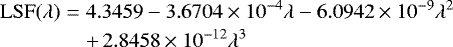 (A.1)
(A.1)
where λ is the wavelength in Å. This LSF has a minimum of 2.45 Å FWHM, narrower than the internal width of the MILES (Falcón-Barroso et al. 2011) and MIUSCAT spectral libraries.
As further input parameters we set starting values for the kinematics to have the central velocity value of the Antennae and a σcont = 75 km s−1 for the stars and σgas= 45 km s−1 for the emissionlines.
A.1 Full datacube analysis
When dealing with the full datacube of the central Antennae, we first improved the S/N to get reliable fits, and produced data with continuum S/N of 30, 50, 100, and 250 with the Voronoi binning technique (Cappellari & Copin 2003). We use the two high-S/N sets to compute initial velocities, and combined and spatially smooth the results, separately for stars and gas. Then we run pPXF on the lower S/N data, using the maps with initial velocities as input. In this case, the emission line templates are mainly used to improve the continuum fit, instead of masking the spectral regions around the emission lines. The stellar fit is then subtracted from the data to produce a cube that contains only the emission of ionized gas, and where the Balmer lines should be corrected for underlying absorption. We can then estimate S/N of the Hα emission line in this continuum-free cube and Voronoi-bin that to a S/N adapted to the strength of the gas emission. We note that this binning will have a different spatial layout than the continuum binning to the same target S/N.
As this sequence of analysis steps is complex and the resulting continuum-free cube is not free of artifacts, we aim to do as many analysis steps on the original cubes as possible, and only use the continuum-free cube where technically necessary, and to cross-check the results.
Since the southern region consists largely of sky background and contains several bright foreground stars as well as a number of background galaxies, and since the object itself is non-contiguous, the Voronoi scheme does not create a sensible two-dimensional grid. We therefore did not attempt to create a similar continuum-free cube for the southern field.
A.2 Individual spectra
When analyzing integrated spectra (e.g., the HII regions) instead, no extra spatial binning is required. The pPXF result then gives us the kinematical data of each spectrum, and the continuum-corrected best-fit emission line fluxes. To also derive corresponding error estimates, we use the fit residuals of the spectrum. To get a reasonable estimate of the total noise for each emission line, we compute the sliding standard deviation of the residuals over a width of 6 wavelength pixels (about 2 × FWHM)15. This noise array is then used to iterate 100 Monte-Carlo fits with pPXF, leaving the best-fit continuum and the kinematics constant but computing new emission line fluxes for every iteration.
References
- Alonso-Herrero, A., García-Marín, M., Rodríguez Zaurín J., et al. 2010, A&A, 522, A7 [NASA ADS] [CrossRef] [EDP Sciences] [Google Scholar]
- Amram, P., Marcelin, M., Boulesteix, J., & Le Coarer, E. 1992, A&A, 266, 106 [NASA ADS] [Google Scholar]
- Anders, P., & Fritze-v. Alvensleben, U. 2003, A&A, 401, 1063 [NASA ADS] [CrossRef] [EDP Sciences] [Google Scholar]
- Anders, P., Bissantz, N., Fritze-v. Alvensleben, U., & de Grijs, R. 2004, MNRAS, 347, 196 [NASA ADS] [CrossRef] [Google Scholar]
- Anders, P., Kotulla, R., de Grijs, R., & Wicker, J. 2013, ApJ, 778, 138 [NASA ADS] [CrossRef] [Google Scholar]
- Bacon, R., Accardo, M., Adjali, L., et al. 2010, in Ground-based and Airborne Instrumentation for Astronomy III, Proc. SPIE, 7735 [Google Scholar]
- Bacon, R., Accardo, M., Adjali, L., et al. 2012, The Messenger, 147, 4 [NASA ADS] [Google Scholar]
- Bastian, N., Emsellem, E., Kissler-Patig, M., & Maraston, C. 2006, A&A, 445, 471 [NASA ADS] [CrossRef] [EDP Sciences] [Google Scholar]
- Bastian, N., Trancho, G., Konstantopoulos, I. S., & Miller, B. W. 2009, ApJ, 701, 607 [NASA ADS] [CrossRef] [Google Scholar]
- Bigiel, F., Leroy, A. K., Blitz, L., et al. 2015, ApJ, 815, 103 [NASA ADS] [CrossRef] [Google Scholar]
- Bournaud, F., Duc, P.-A., Amram, P., Combes, F., & Gach, J.-L. 2004, A&A, 425, 813 [NASA ADS] [CrossRef] [EDP Sciences] [Google Scholar]
- Brandl, B. R., Clark, D. M., Eikenberry, S. S., et al. 2005, ApJ, 635, 280 [NASA ADS] [CrossRef] [Google Scholar]
- Brandl, B. R., Snijders, L., den Brok, M., et al. 2009, ApJ, 699, 1982 [NASA ADS] [CrossRef] [Google Scholar]
- Calzetti, D., Armus, L., Bohlin, R. C., et al. 2000, ApJ, 533, 682 [NASA ADS] [CrossRef] [Google Scholar]
- Campbell, A., & Willner, S. P. 1989, AJ, 97, 995 [NASA ADS] [CrossRef] [Google Scholar]
- Cappellari, M., & Copin, Y. 2003, MNRAS, 342, 345 [NASA ADS] [CrossRef] [Google Scholar]
- Cappellari, M.& Emsellem, E. 2004, PASP, 116, 138 [NASA ADS] [CrossRef] [Google Scholar]
- Chandar, R., Whitmore, B. C., Dinino, D., et al. 2016, ApJ, 824, 71 [NASA ADS] [CrossRef] [Google Scholar]
- Conselice, C. J. 2003, ApJS, 147, 1 [NASA ADS] [CrossRef] [Google Scholar]
- Dopita, M. A. & Sutherland, R. S. 1995, ApJ, 455, 468 [NASA ADS] [CrossRef] [Google Scholar]
- Faisst, A. L. 2016, ApJ, 829, 99 [NASA ADS] [CrossRef] [Google Scholar]
- Falcón-Barroso, J., Sánchez-Blázquez, P., Vazdekis, A., et al. 2011, A&A, 532, A95 [NASA ADS] [CrossRef] [EDP Sciences] [Google Scholar]
- Fensch, J., Duc, P.-A., Weilbacher, P. M., Boquien, M., & Zackrisson, E. 2016, A&A, 585, A79 [NASA ADS] [CrossRef] [EDP Sciences] [Google Scholar]
- Ferguson, A. M. N., Wyse, R. F. G., & Gallagher, J. S. 1996, AJ, 112, 2567 [NASA ADS] [CrossRef] [Google Scholar]
- Fouesneau, M., & Lançon, A. 2010, A&A, 521, A22 [NASA ADS] [CrossRef] [EDP Sciences] [Google Scholar]
- Fouesneau, M., Lançon, A., Chandar, R., & Whitmore, B. C. 2012, ApJ, 750, 60 [NASA ADS] [CrossRef] [Google Scholar]
- Gaia Collaboration (Brown, A. G. A., Vallenari, A., et al.) 2016, A&A, 595, A2 [NASA ADS] [CrossRef] [EDP Sciences] [Google Scholar]
- Gilbert, A. M., & Graham, J. R. 2007, ApJ, 668, 168 [NASA ADS] [CrossRef] [Google Scholar]
- Haas, M., Chini, R., & Klaas, U. 2005, A&A, 433, L17 [NASA ADS] [CrossRef] [EDP Sciences] [Google Scholar]
- Haffner, L. M., Dettmar, R.-J., Beckman, J. E., et al. 2009, Rev. Mod. Phys., 81, 969 [NASA ADS] [CrossRef] [Google Scholar]
- Heckman, T. M., Dahlem, M., Lehnert, M. D., et al. 1995, ApJ, 448, 98 [NASA ADS] [CrossRef] [Google Scholar]
- Heidt, J., Appenzeller, I., Gabasch, A., et al. 2003, A&A, 398, 49 [NASA ADS] [CrossRef] [EDP Sciences] [Google Scholar]
- Heydari-Malayeri, M., Charmandaris, V., Deharveng, L., Rosa, M. R., & Zinnecker, H. 1999, A&A, 347, 841 [NASA ADS] [Google Scholar]
- Hibbard, J., van der Hulst, J., Barnes, J., & Rich, R. 2001, AJ, 122, 2969 [NASA ADS] [CrossRef] [Google Scholar]
- Hibbard, J. E., Bianchi, L., Thilker, D. A., et al. 2005, ApJ, 619, L87 [NASA ADS] [CrossRef] [Google Scholar]
- Hoopes, C. G., & Walterbos, R. A. M. 2003, ApJ, 586, 902 [NASA ADS] [CrossRef] [Google Scholar]
- Ivison, R. J., Smail, I., Amblard, A., et al. 2012, MNRAS, 425, 1320 [NASA ADS] [CrossRef] [Google Scholar]
- Izotov, Y. I., Orlitová, I., Schaerer, D., et al. 2016a, Nature, 529, 178 [NASA ADS] [CrossRef] [Google Scholar]
- Izotov, Y. I., Schaerer, D., Thuan, T. X., et al. 2016b, MNRAS, 461, 3683 [NASA ADS] [CrossRef] [Google Scholar]
- Jaskot, A. E., & Oey, M. S. 2013, ApJ, 766, 91 [NASA ADS] [CrossRef] [Google Scholar]
- Karl, S. J., Naab, T., Johansson, P. H., et al. 2010, ApJ, 715, L88 [NASA ADS] [CrossRef] [Google Scholar]
- Kassin, S. A., Frogel, J. A., Pogge, R. W., Tiede, G. P., & Sellgren, K. 2003, AJ, 126, 1276 [NASA ADS] [CrossRef] [Google Scholar]
- Kehrig, C., Monreal-Ibero, A., Papaderos, P., et al. 2012, A&A, 540, A11 [NASA ADS] [CrossRef] [EDP Sciences] [Google Scholar]
- Kennicutt, R. 1998, ARA&A, 36, 189 [Google Scholar]
- Kewley, L. J., Dopita, M. A., Sutherland, R. S., Heisler, C. A., & Trevena, J. 2001, ApJ, 556, 121 [Google Scholar]
- Kotulla, R., Fritze, U., Weilbacher, P., & Anders, P. 2009, MNRAS, 396, 462 [NASA ADS] [CrossRef] [Google Scholar]
- Kreckel, K., Blanc, G. A., Schinnerer, E., et al. 2016, ApJ, 827, 103 [NASA ADS] [CrossRef] [Google Scholar]
- Kroupa, P. 2002, Science, 295, 82 [NASA ADS] [CrossRef] [PubMed] [Google Scholar]
- Lacey, C., & Cole, S. 1993, MNRAS, 262, 627 [NASA ADS] [CrossRef] [Google Scholar]
- Lardo, C., Davies, B., Kudritzki, R.-P., et al. 2015, ApJ, 812, 160 [NASA ADS] [CrossRef] [Google Scholar]
- Lee, J. C., Veilleux, S., McDonald, M., & Hilbert, B. 2016, ApJ, 817, 177 [NASA ADS] [CrossRef] [Google Scholar]
- Lehnert, M. D., & Heckman, T. M. 1996, ApJ, 462, 651 [NASA ADS] [CrossRef] [Google Scholar]
- Leitet, E., Bergvall, N., Hayes, M., Linné, S., & Zackrisson, E. 2013, A&A, 553, A106 [NASA ADS] [CrossRef] [EDP Sciences] [Google Scholar]
- Leitherer, C., Schaerer, D., Goldader, J., et al. 1999, ApJS, 123, 3 [NASA ADS] [CrossRef] [Google Scholar]
- Leitherer, C., Ortiz Otálvaro, P. A., Bresolin, F., et al. 2010, ApJS, 189, 309 [NASA ADS] [CrossRef] [Google Scholar]
- Leitherer, C., Hernandez, S., Lee, J. C., & Oey, M. S. 2016, ApJ, 823, 64 [NASA ADS] [CrossRef] [Google Scholar]
- Levesque, E. M., Leitherer, C., Ekstrom, S., Meynet, G., & Schaerer, D. 2012, ApJ, 751, 67 [NASA ADS] [CrossRef] [Google Scholar]
- Luridiana, V., Morisset, C., & Shaw, R. A. 2015, A&A, 573, A42 [NASA ADS] [CrossRef] [EDP Sciences] [Google Scholar]
- Madsen, G. J., Reynolds, R. J., & Haffner, L. M. 2006, ApJ, 652, 401 [NASA ADS] [CrossRef] [Google Scholar]
- Mathis, J. S. 2000, ApJ, 544, 347 [NASA ADS] [CrossRef] [Google Scholar]
- Mengel, S., Lehnert, M. D., Thatte, N., & Genzel, R. 2005, A&A, 443, 41 [NASA ADS] [CrossRef] [EDP Sciences] [Google Scholar]
- Mirabel, I., Dottori, H., & Lutz, D. 1992, A&A, 256, L19 [NASA ADS] [Google Scholar]
- Mirabel, I. F., Vigroux, L., Charmandaris, V., et al. 1998, A&A, 333, L1 [NASA ADS] [Google Scholar]
- Monreal-Ibero, A., Arribas, S., & [Google Scholar]
- Monreal-Ibero, A., Arribas, S., Colina, L., et al. 2010, A&A, 517, A28 [NASA ADS] [CrossRef] [EDP Sciences] [Google Scholar]
- Munari, U., Sordo, R., Castelli, F., & Zwitter, T. 2005, A&A, 442, 1127 [NASA ADS] [CrossRef] [EDP Sciences] [Google Scholar]
- Nakajima, K. & Ouchi, M. 2014, MNRAS, 442, 900 [NASA ADS] [CrossRef] [Google Scholar]
- Niederhofer, F., Hilker, M., Bastian, N., & Ercolano, B. 2016, A&A, 592, A47 [NASA ADS] [CrossRef] [EDP Sciences] [Google Scholar]
- Osterbrock, D. E. & Ferland, G. J. 2005, Astrophysics of Gaseous Nebulae and Active Galactic Nuclei, 2nd edn. (University Science Books) [Google Scholar]
- Papaderos, P., Gomes, J. M., Vílchez, J. M., et al. 2013, A&A, 555, L1 [NASA ADS] [CrossRef] [EDP Sciences] [Google Scholar]
- Pellegrini, E. W., Oey, M. S., Winkler, P. F., et al. 2012, ApJ, 755, 40 [NASA ADS] [CrossRef] [Google Scholar]
- Pleuss, P., Heller, C., & Fricke, K. 2000, A&A, 361, 913 [NASA ADS] [Google Scholar]
- Renaud, F., Bournaud, F., & Duc, P.-A. 2015, MNRAS, 446, 2038 [NASA ADS] [CrossRef] [Google Scholar]
- Rich, J. A., Kewley, L. J., & Dopita, M. A. 2011, ApJ, 734, 87 [NASA ADS] [CrossRef] [Google Scholar]
- Rossa, J., & Dettmar, R.-J. 2003, A&A, 406, 493 [NASA ADS] [CrossRef] [EDP Sciences] [Google Scholar]
- Rossa, J., Dettmar, R.-J., Walterbos, R. A. M., & Norman, C. A. 2004, AJ, 128, 674 [NASA ADS] [CrossRef] [Google Scholar]
- Rubin, V. C., Ford, Jr. W. K., & D’Odorico, S. 1970, ApJ, 160, 801 [NASA ADS] [CrossRef] [Google Scholar]
- Salpeter, E. 1955, ApJ, 121, 161 [Google Scholar]
- Sanders, D., & Mirabel, I. 1996, ARA&A, 34, 749 [NASA ADS] [CrossRef] [Google Scholar]
- Sandin, C. 2014, A&A, 567, A97 [NASA ADS] [CrossRef] [EDP Sciences] [Google Scholar]
- Sandin, C. 2015, A&A, 577, A106 [NASA ADS] [CrossRef] [EDP Sciences] [Google Scholar]
- Sandin, C., Becker, T., Roth, M. M., et al. 2010, A&A, 515, A35 [NASA ADS] [CrossRef] [EDP Sciences] [Google Scholar]
- Sandin, C., Weilbacher, P., Tabataba-Vakili, F., Kamann, S., & Streicher, O. 2012, in Proc. SPIE, 8451, Software and Cyberinfrastructure for Astronomy II [Google Scholar]
- Schaerer, D., & de Koter, A. 1997, A&A, 322, 598 [NASA ADS] [Google Scholar]
- Schaye, J., Crain, R. A., Bower, R. G., et al. 2015, MNRAS, 446, 521 [Google Scholar]
- Schirm, M. R. P., Wilson, C. D., Parkin, T. J., et al. 2014, ApJ, 781, 101 [NASA ADS] [CrossRef] [Google Scholar]
- Schweizer, F., Burns, C. R., Madore, B. F., et al. 2008, AJ, 136, 1482 [NASA ADS] [CrossRef] [Google Scholar]
- Scoville, N. Z., Polletta, M., Ewald, S., et al. 2001, AJ, 122, 3017 [NASA ADS] [CrossRef] [Google Scholar]
- Skrutskie, M. F., Cutri, R. M., Stiening, R., et al. 2006, AJ, 131, 1163 [NASA ADS] [CrossRef] [Google Scholar]
- Smith, L. J., Norris, R. P. F., & Crowther, P. A. 2002, MNRAS, 337, 1309 [NASA ADS] [CrossRef] [Google Scholar]
- Soto, K. T., Martin, C. L., Prescott, M. K. M., & Armus, L. 2012, ApJ, 757, 86 [NASA ADS] [CrossRef] [Google Scholar]
- Stasińska, G., Izotov, Y., Morisset, C., & Guseva, N. 2015, A&A, 576, A83 [NASA ADS] [CrossRef] [EDP Sciences] [Google Scholar]
- Steinmetz, M., & Navarro, J. F. 2002, New Astronomy, 7, 155 [NASA ADS] [CrossRef] [Google Scholar]
- Tacconi, L. J., Genzel, R., Smail, I., et al. 2008, ApJ, 680, 246 [NASA ADS] [CrossRef] [PubMed] [Google Scholar]
- Toomre, A., & Toomre, J. 1972, ApJ, 178, 623 [NASA ADS] [CrossRef] [Google Scholar]
- Vazdekis, A., Ricciardelli, E., Cenarro, A. J., et al. 2012, MNRAS, 424, 157 [NASA ADS] [CrossRef] [Google Scholar]
- Ventou, E., Contini, T., Bouché, N., et al. 2017, A&A, 608, A9 [NASA ADS] [CrossRef] [EDP Sciences] [Google Scholar]
- Vogelsberger, M., Genel, S., Springel, V., et al. 2014, MNRAS, 444, 1518 [NASA ADS] [CrossRef] [Google Scholar]
- Voges, E. S., & Walterbos, R. A. M. 2006, ApJ, 644, L29 [NASA ADS] [CrossRef] [Google Scholar]
- Voges, E. S., Oey, M. S., Walterbos, R. A. M., & Wilkinson, T. M. 2008, AJ, 135, 1291 [NASA ADS] [CrossRef] [Google Scholar]
- Weilbacher, P. 2015, in Science Operations 2015: Science Data Management – An ESO/ESA Workshop, ESO Garching, (https://www.eso.org/sci/ meetings/2015/SciOps2015.html) [Google Scholar]
- Weilbacher, P. M., Duc, P.-A., & Fritze-von Alvensleben, U. 2003, A&A, 397, 545 [NASA ADS] [CrossRef] [EDP Sciences] [Google Scholar]
- Weilbacher, P. M., Streicher, O., Urrutia, T., et al. 2012, in Proc. SPIE, 8451, Software and Cyberinfrastructure for Astronomy II [Google Scholar]
- Weilbacher, P. M., Streicher, O., Urrutia, T., et al. 2014, in ASP Conf. Ser., Astronomical Data Analysis Software and Systems XXIII, eds. N. Manset, & P. Forshay, 485, 451 [NASA ADS] [Google Scholar]
- Weilbacher, P. M., Monreal-Ibero, A., Kollatschny, W., et al. 2015a, A&A, 582, A114 [NASA ADS] [CrossRef] [EDP Sciences] [Google Scholar]
- Weilbacher, P. M., Monreal-Ibero, A., Mc Leod, A. F., et al. 2015b, The Messenger, 162, 37 [NASA ADS] [Google Scholar]
- White, S., & Rees, M. 1978, MNRAS, 183, 341 [NASA ADS] [CrossRef] [Google Scholar]
- Whitmore, B., Zhang, Q., Leitherer, C., et al. 1999, AJ, 118, 1551 [NASA ADS] [CrossRef] [Google Scholar]
- Whitmore, B. C., Gilmore, D., Leitherer, C., et al. 2005, AJ, 130, 2104 [NASA ADS] [CrossRef] [Google Scholar]
- Whitmore, B. C., Chandar, R., Schweizer, F., et al. 2010, AJ, 140, 75 [Google Scholar]
- Whitmore, B. C., Brogan, C., Chandar, R., et al. 2014, ApJ, 795, 156 [NASA ADS] [CrossRef] [Google Scholar]
- Zaragoza-Cardiel, J., Font, J., Beckman, J. E., et al. 2014, MNRAS, 445, 1412 [NASA ADS] [CrossRef] [Google Scholar]
- Zastrow, J., Oey, M. S., Veilleux, S., & McDonald, M. 2013, ApJ, 779, 76 [NASA ADS] [CrossRef] [Google Scholar]
- Zhang, K., Yan, R., Bundy, K., et al. 2017, MNRAS, 466, 3217 [NASA ADS] [CrossRef] [Google Scholar]
- Zurita, A., Beckman, J. E., Rozas, M., & Ryder, S. 2002, A&A, 386, 801 [NASA ADS] [CrossRef] [EDP Sciences] [Google Scholar]
Another operational update of the pipeline was discussed in Weilbacher (2015).
The NASA/IPAC Extragalactic Database (NED) is operated by the Jet Propulsion Laboratory, California Institute of Technology, under contract with the National Aeronautics and Space Administration.
By “ridge” we refer to the center of the tidal tail that in Fig. 3 is highlighted by the outermost Hα contours in the left of the map.
We assume that the vertical axis of Fig. 6 of Hibbard et al. (2001) is supposed to have coordinates −18°59′, −19°00′, −19°01′, and −19°02′, since the 10′ distances between the southern axis ticks do not make sense.
Since the exposure time of the standard stars is set to give optimal signal-to-noise ratio (S/N) without saturation, it is not surprising that we did not find any brighter, isolated point sources that were observed with MUSE in a similar setup and with higher S/N in the outer parts of the PSF. So we cannot currently derive any better PSF estimate.
p3d has the advantage of being able to fit line profiles on log-sampled spectra and can make use of Voronoi bins, while being extremely fast compared to other tools like pPXF. It is available from http://p3d.sourceforge.net/.
That leaking LyC photons from HII regions contribute to the DIG in the Antennae was already mentioned by Whitmore et al. (2005), but their argument seems to contradict what these photoionization models show. However, they were only referring to DIG immediately surrounding the brightest star cluster complexes.
Available as the astrodendro Python package from http://dendrograms.org
For bright stars, the continuum subtraction in the detection image was imperfect, so some of them were false HII region detections in the dendrogram.
The equivalent width of the stellar absorption is larger for Hβ than Hα. With narrow-band filters one cannot correct for this effect, hence this procedure underestimates the emission line fluxes, more so for Hβ. In regions where this absorption is significant relative to the emission line, this can lead to an overestimate of the extinction.
We note that since the dominant fraction of the southern field is blank sky and contains neither clumpy nor diffuse Hα line emission, the value given for this field depends strongly on how well the sky could be subtracted in the Hα wavelength region as well as on the level of artifacts left after continuum subtraction. The diffuse flux estimate and hence diffuse fraction therefore comes with a significant systematic error and should be understood as 10 ± 5%.
While the Whitmore et al. (2010) publication comes with a selection of tables of most noteworthy objects, the full table of 60 790 objects was sent to us by B. Whitmore by private mail. We corrected the coordinates in this table by Δα = −1.′′345 and Δδ = +1.′′607 to match the astrometric calibration of the MUSE data.
We use solar metallicity models for comparison, since Bastian et al. (2006) and Lardo et al. (2015) estimate approximately solar metallicity for the central part of the Antennae. As regions in the outskirts are likely to have lower metal abundances, the solar estimate of the LyC photon flux represents a lower limit to the real LyC flux.
Here, we use the conservative estimate using the GALEV code without dust reddening, since the extinction in the southern tail is very low. The standard deviation of fesc among these regions is 22%, the median 83%.
The MUSE data carries a variance estimate which provides a good estimate of the per voxel noise in the presence of significant background. However, this propagated variance is correlated to neighboring voxels due to the cube reconstruction, and therefore one cannot trust its absolute value when binning spectra over a region. Hence, the effective noise that we use here should provide a better error estimate.
All Tables
All Figures
|
Fig. 1 Antennae as seen on the blue Digital Sky Survey, version 2. The light red and light blue boxes show the outer edges of the MUSE coverage as used in all further plots. The red contours mark arbitrary continuum levels derived from a smoothed HST ACS image in the F814W filter in the central interacting galaxy. The two galaxy nuclei can be used to relate their location in other figures in this paper. The blue contours are similarly derived from HST data in the region near the tip of the southern tidal tail, they mark mostly foreground stars and background objects. The two bright stars in this region can be used to relate the location of this field to the other figures in this paper. This region is sometimes called NGC 4038 S in the literature; here, we use the term south or southern to describe it. |
| In the text | |
|
Fig. 2 Inverse gray-scale map of the relative weights of the data of the MUSE data of the Antennae. In this representation, the deepest regions appear black while those parts of the data only covered by exposures taken in poor conditions appear light gray. In color, boxes representing the MUSE fields (each approx. 1′× 1′ in size) are shown, with the annotated field designation and a cross marking the field center. The white contours are similar to the continuum levels shown in Fig. 1. Panel a: pointings of the central Antennae; panel b: pointings around the tip of the southern tidal tail are presented. Panel b: a removed satellite trail that decreased the effective exposure time is marked with a dashed cyan arrow. |
| In the text | |
|
Fig. 3 Continuum-subtracted Hα flux maps for the central (panel a) and the southern (panel b) region, as produced by the narrow-band technique (see text). The common color scaling (color bar on the right) was chosen to highlight faint features. The black-to-gray contours denote the Hα flux levels, smoothed by a 3-pixel Gaussian, of 2.50 × 10⁻¹⁷, 1.25 × 10⁻¹⁶, 2.50 × 10⁻¹⁶, 1.25 × 10⁻¹⁵, 2.50 × 10⁻¹⁵, and 1.25 × 10⁻¹⁴ erg s−1 cm−2 arcsec−2; since the emission in the southern region is fainter, not all contours are visible in panel b. The green contours highlight continuum features and are identical to those shown in Fig. 1. In panel b, the blue circles and corresponding roman numerals denote the detections by Mirabel et al. (1992) with coordinates from Hibbard et al. (2001), while the red circles and arabic numerals are detections by Bournaud et al. (2004). |
| In the text | |
|
Fig. 4 Radial profiles of the Hα surface brightness compared to the point spread function (PSF) as derived from two typical standard star observations. Panel a: Hα flux map from Gaussian line fits to the emission line, comparable to Fig. 3a, but with radial extraction cuts marked and the corresponding Hα peaks numbered. Low-level patterns caused by the correlated noise in the MUSE cubes are marked with arrows. Panel b: radial flux distribution outwards from the HII regions. The markers in the map and the corresponding profiles are shown with the same color. The PSFs derived from the standard stars are shown as elliptical profiles with error bars and triple Moffat fits. |
| In the text | |
|
Fig. 5 Velocity derived from the Hα emission line in the central field of the Antennae. The velocities are corrected to the solar-system barycenter and are computed over bins of S∕N ~ 30 (see text). The green lines are the same HST broad-band contours as in Fig. 1. |
| In the text | |
|
Fig. 6 Diagnostic diagrams showing the properties of the faint ionized gas. The radius of the three data points in each panel scales linearly to the square-root of the area, and the error bars aresmaller than the size of the points. The color is coded according to the average Hα surface brightness. The solid line indicates the nominal photoionization limit of Kewley et al. (2001). |
| In the text | |
|
Fig. 7 Flux ratio maps; [N II]6548.84/Hα (panel a), [S II]6716.31/Hα (panel b). Both are Voronoi-binned to S∕NHα ~ 30. Overplotted are the same Hα contours as in Fig. 3a and broad-band levels as in Fig. 1. Features discussed in the text are marked with arrows. |
| In the text | |
|
Fig. 8 H II regions detected in the Antennae using the ASTRODENDRO package. The common color-scale gives the Hα flux of each region. Left panel: central region; right panel: southern region. The contours are the same broad-band levels as in Fig. 1. H II regions whose spectra are displayed in Fig. 9 are marked. |
| In the text | |
|
Fig. 9 Three example spectra of H II regions: c1665 is located near the NGC4038 nucleus, c349 is in the tidal tail of the central field, s9 is in the southern field. The corresponding regions are annotated in Fig. 8. In each upper panel, the black line shows the extracted data, the red line is the continuum fit and the blue lines represent the fit to gas emission. The green points with error bars in the lower panels show the residuals of the pPXF fit. |
| In the text | |
|
Fig. 10 Hα luminosity function for the HII regions detected in the Antennae using the astrodendro package. The bold blue lines (solid: central region, dashed: southern field) show the luminosity histogram in our MUSE data of the Antennae, after correction for internal extinction. The red solid line shows the luminosity function of Zaragoza-Cardiel et al. (2014). |
| In the text | |
|
Fig. 11 H II regions detected in the central Antennae. Here, the color indicates the Lyman-continuum escape fraction fesc, estimated bycomparing Hα luminosity and illuminating young star cluster(s). All colored regions have a positive escape fraction, other regions are filled light gray. The contours are the same broad-band levels as in Fig. 1, and the dashed dark-green line shows the approximate limit of the HST imaging. |
| In the text | |
|
Fig. 12 Ionization-parameter-sensitive line ratios against Lyman-continuum escape fraction (fesc) for our sample of HII regions. Panel a: line ratio [O iii]5007/[O I]6300; panel b: [S iii]9068.9531/[S II]6716.31, and panel c: [O iii]5007//[S II]6716.31. In all plots, the blue points are the results using the GALEV model while the red points shows the escape fraction computed using SB99. 1σ ranges of the statistical error of both axes are plotted as gray lines for the GALEV results. Violet points at the left border are those regions which were found to be optically thick. Horizontal dashed lines denote lower limits of the line ratios with high escape fraction, as discussed in the text. |
| In the text | |
Current usage metrics show cumulative count of Article Views (full-text article views including HTML views, PDF and ePub downloads, according to the available data) and Abstracts Views on Vision4Press platform.
Data correspond to usage on the plateform after 2015. The current usage metrics is available 48-96 hours after online publication and is updated daily on week days.
Initial download of the metrics may take a while.