| Issue |
A&A
Volume 611, March 2018
|
|
|---|---|---|
| Article Number | A49 | |
| Number of page(s) | 12 | |
| Section | The Sun | |
| DOI | https://doi.org/10.1051/0004-6361/201628436 | |
| Published online | 22 March 2018 | |
Mass and energy supply of a cool coronal loop near its apex★
1
School of Earth and Space Sciences, Peking University,
100871 Beijing,
PR China
e-mail: This email address is being protected from spambots. You need JavaScript enabled to view it.
2
Max-Plank-Institut für Sonnensystemforschung,
Justus-von-Liebig-Weg 3,
37077 Göttingen,
Germany
3
Key Laboratory of Earth and Planetary Physics, Institute of Geology and Geophysics, Chinese Academy of Sciences,
Beijing 100029,
PR China
4
Shandong Provincial Key Laboratory of Optical Astronomy and Solar-Terrestrial Environment,
School of Space Science and Physics, Shandong University,
250100 Weihai,
PR China
Received:
5
March
2017
Accepted:
26
September
2017
Abstract
Context. Different models for the heating of solar corona assume or predict different locations of the energy input: concentrated at the footpoints, at the apex, or uniformly distributed. The brightening of a loop could be due to the increase in electron density ne, the temperature T, or a mixture of both.
Aim. We investigate possible reasons for the brightening of a cool loop at transition region temperatures through imaging and spectral observation.
Methods. We observed a loop with the Interface Region Imaging Spectrograph (IRIS) and used the slit-jaw images together with spectra taken at a fixed slit position to study the evolution of plasma properties in and below the loop. We used spectra of Si iv, which forms at around 80 000 K in equilibrium, to identify plasma motions and derive electron densities from the ratio of inter-combination lines of O IV. Additional observations from the Solar Dynamics Observatory (SDO) were employed to study the response at coronal temperatures (Atmospheric Imaging Assembly, AIA) and to investigate the surface magnetic field below the loop (Helioseismic and Magnetic Imager, HMI).
Results. The loop first appears at transition region temperatures and later also at coronal temperatures, indicating a heating of the plasma in the loop. The appearance of hot plasma in the loop coincides with a possible accelerating upflow seen in Si IV, with the Doppler velocity shifting continuously from ~−70 km s−1 to ~−265 km s−1. The 3D magnetic field lines extrapolated from the HMI magnetogram indicate possible magnetic reconnection between small-scale magnetic flux tubes below or near the loop apex. At the same time, an additional intensity enhancement near the loop apex is visible in the IRIS slit-jaw images at 1400 Å. These observations suggest that the loop is probably heated by the interaction between the loop and the upflows, which are accelerated by the magnetic reconnection between small-scale magnetic flux tubes at lower altitudes. Before and after the possible heating phase, the intensity changes in the optically thin (Si IV) and optical thick line (C II) are mainly contributed by the density variation without significant heating.
Conclusions. We therefore provide evidence for the heating of an envelope loop that is affected by accelerating upflows, which are probably launched by magnetic reconnection between small-scale magnetic flux tubes underneath the envelope loop. This study emphasizes that in the complex upper atmosphere of the Sun, the dynamics of the 3D coupled magnetic field and flow field plays a key role in thermalizing 1D structures such as coronal loops.
Key words: line: profiles / magnetic reconnection / Sun: corona / Sun: transition region / techniques: spectroscopic / Sun: UV radiation
An animation associated to Fig. 1 is available at https://www.aanda.org
© ESO 2018
1 Introduction
Coronal loops that appear as bright arc-like features with two footpoints located in opposite magnetic polarities are the basic building blocks of the solar corona. They are visible at a wide range of temperatures, from about 105 K up to a few 107 K, and usually carry denser material than the surrounding environment (Reale 2014).
The heating of coronal loops may occur at various places in magnetic loops: mainly at the loop apex or at the footpoint, but it can also be uniformly distributed. Early models of loop heating typically assumed a uniform heating along the loop (e.g., Rosner et al. 1978; Chiuderi et al. 1981). By comparing the temperature profile along the loop from observations with the profile obtained from theoretical models based on a different form of heating, Priest et al. (1998, 2000) tended to support the scenario of uniform heating for the observed loops.
However, other observations suggested different results. Kano & Tsuneta (1996) found that the loops were frequently heated at the apex,as inferred from the triangular temperature distribution along the loop. Reale (2002) compared the intensity profiles along the loops synthesized from loop models and those obtained from observations and found that the hot (≈ 4 MK) loops were preferentially heated at the loop apex.
Aschwanden et al. (2001) found that the heating of loops seen in the extreme ultraviolet (EUV) was probably restricted to the footpoint. They employed the observed flat temperature profiles as an argument. Aschwanden et al. (2007) and Klimchuk (2006) gave a collection of reasons why heating should be footpoint dominated. More recent 3D magnetohydrodynamic (MHD) models of the corona all show that the heating is concentrated at the footpoints (e.g., Hansteen et al. 2010; Bingert & Peter 2011). This is true not only on average, but also for individual field lines (van Wettum et al. 2013). As indicated by the simulations of Gudiksen & Nordlund (2002), the heating at the footpoints of loops is driven by magnetoconvection. As suggested by Buchlin et al. (2007), the expansion of the flux tube and the general drop in the average magnetic field with height are two reasons for enhanced heating at the footpoints. Still, if the magnetic field of a loop interacts with the surrounding structures, as in the case of an emerging-flux situation, the heating near the apex of the loop might also be significant (Chen et al. 2014). The role of 3D numerical experiments for understanding the spatial and temporal variability of coronal heating is summarized in Peter (2015).
Observations of the corona can only provide information on the flux and energy of the recorded photons. No direct information is available on the actual plasma properties, such as temperature or density, which have to be inferred from the observations. In general, the brightening of coronal loops could be due to the increase in the (electron) density ne or the temperatureT, or both. Under optical thin conditions, the emission is proportional to  and a contribution function, often named G(T), which depends on T and is (mainly) governed by atomic properties (e.g., Mariska 1992). Under optically thick conditions, the emission of a line is proportional to ne and again a contribution function depending on T (e.g., Athay 1966; Nagai 1980; Carlsson & Leenaarts 2012). As a rule of thumb, the transition from optically thick to optical thin occurs at around 104.6 K (Matsumoto & Suzuki 2014). However, self-absorption has recently also been observed in lines forming above this threshold, that is, in the Si IV line, which forms at around 104.8 K (Yan et al. 2015), but this may not be a widespread phenomenon at quiet times.
In terms of understanding the physics of the intensity variation, it is pivotal to understand whether, for instance, an increase in intensity is due to a density rise alone, a change of temperature alone, or due to a mixture of both. This can be investigated by deriving the density in the source region of a line and then comparing this to the variation of the line intensity. For example, if the intensity change of an optically thin line is proportional to the change in  , then this increasein brightness would most probably be due to a pure density increase without a noticeable temperature change.
In this study we investigate a small cool transition region loop that shows additional brightening near its apex as observed by the Interface Region Imaging Spectrograph (IRIS; De Pontieu et al. 2014). We selected this particular case because in addition to the interesting feature of the brightening occurring from the middle of the loop, we find very interesting line profiles of Si IV thatpromise to provide new insights. In addition, the simultaneously observed lines of O IV are bright enough to provide diagnostics for the (electron) density. Furthermore, the combination of optically thick (C II at ≈ 104.4 K) and thin lines (Si IV at ≈104.8 K, O IV at ≈105.2 K) gives further diagnostic capabilities to distinguish the roles of density and temperature in the brightening of the structure. This is only a single but very interesting case that requires follow-up studies of more cool loops.
2 Observations
IRIS provides high temporal and spatial resolution spectra and slit-jaw images (SJI) of the chromosphere and transition region (De Pontieu et al. 2014). In this study, we focus on an emerging active region observed by IRIS from 09:06 and 09:43 UT on December 06, 2013. During this observation, data were recorded in sit-and-stare mode (i.e., with the slit at a fixed position on the Sun), with an exposure time of 4.0 s, a spectral resolution of ~0.03 Å, and a spatial sampling of 0.167″ per pixel. The SJI, with an exposure time of 4.0 s and a field-of-view (FOV) of 121″ × 128″, are obtained at four wavelengths. For imaging we mainly used SJI at 1400 Å, which show a mixture of continuum emission and Si IV emission from the transition region. For the spectroscopic analysis we concentrated on the line profile of Si IV at 1394 Å and 1403 Å, the C II lines at 1334 Å and 1335 Å, and the intercombination lines of O IV at 1400 Å and 1401 Å to investigate the evolution of a brightening loop. The cadence was 5 s for the spectral observations and 17 s for the imaging. The line ratio of the two O IV lines was used to estimate the electron density.
We complemented these observations with data from AIA (Lemen et al. 2012) channels showing coronal plasma from 0.7 MK to 2 MK (131 Å, 171 Å, 193 Å, 211 Å) and even hotter plasma up to several MK (335 Å, 94 Å). A detailed description of the temperature coverage of AIA can be found in Boerner et al. (2012). The 94 Å channel is composed of a hot component contributed by Fe xviii 93.92 Å (7.1 MK) and a warm component. The contribution of Fe xviii 93.92 Å is obtained by I94 − I94w (Li et al. 2015), where I94w is estimated by an empirical correction (Warren et al. 2012; Ugarte-Urra & Warren 2014). In addition, we used the 1600 and 1700 Å channels. The 1700 channel contains continuum from near the temperature minimum (Vernazza et al. 1981). The 1600 channel also contains emission from the transition region lines of C IV at 1548 and 1550 Å. The cadence for 1600 and 1700 was approximately 24 s. Observations in the other wavelengths have the same cadence of 12 s. We used aia_prep.pro1 to align the observations obtained by AIA in different wavelengths. The line-of-sight (LOS) photospheric magnetic field obtained by HMI (Schou et al. 2012) was used to investigate the corresponding magnetic structure in the photosphere. These magnetograms have a spatial sampling of 0.5″ per pixel and a cadence of 45 s. The context of the observation is shown in Fig. 1 with the FOV of the IRIS SJI marked.
The spatial alignments of the spectra and SJI were obtained using the fiducial marks crossing the slit. The AIA 1600 Å images were used to achieve a coalignment between the IRIS and AIA data and a coalignment between the HMI and AIA data. All images were aligned to the IRIS SJI 1400 Å image obtained at 09:34:25 UT, at which time the profile of the Si IV lines showed a very special shape that we are interested in most.
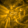 |
Fig. 1 Context of the active region as seen in AIA 193 Å, showing plasma around 1.5 MK. The FOV is 249.6″ × 249.6″ centered at solar X = 50″ and solar Y = −225″. The white dashed and solid rectangles indicate the full FOV of IRIS and the subregion shown in Fig. 2, respectively.See Sect. 2. |
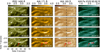 |
Fig. 2 Temporal evolution of the loop. The four rows show snapshots at the indicated times. The columns show the images obtained through the IRIS slit-jaw-images in 1400 Å, the AIA channels at 171 Å and 193 Å, and the Fe xviii (93.92 Å) emission extracted from the AIA channel at 94 Å. The images show plasma at increasing temperatures at below 0.1 MK, 1 MK, 1.5 MK, and at around 7 MK. The black dashed vertical lines indicate the slit position of the IRIS spectrometer. Red arrows point at the loop studied here. Red rectangles show the region of the differential emission measure (DEM) analysis, the result of which is shown in Fig. 7. The color tables shows the data number per pixel on a log 10 scale. The same color table is used for each wavelength channel at the different time steps. The field of view is indicated in Fig. 1 by the solid rectangle. See Sect. 3. A corresponding animation, Animation 1, is available in the online journal. |
3 Time evolution of a heated cool loop
To discuss the timing of the brightening loop, we give times in seconds with respect to 09:32:04 UT. Details of the timing that relate the features observed in various wavelength bands and spectral lines are given in Table A.1. The brightening of the loop starts at 09:32:46 UT and lasts for roughly 2 min in Si IV. The intensity and wing enhancement of the Si IV lines shows a short decrease at 09:33:43 UT, which separates the loop brightening into two main phases.
In phase 1 (from 09:32:46 UT to 09:33:43 UT), the brightening loop is obvious in the transition region emission in SJI 1400 Å, while only the right footpoint of the loop appears in the 0.7 to 2 MK channels of AIA (upper panel in Fig. 2). There is no corresponding feature from even hotter plasma (see Sect. 2). This suggests that the temperature of the loop in phase 1 is relatively low and constrained to below a few 105 K. The blue wing enhancement of Si IV profile is strong, while there is no significant enhancement in the red wing (dark blue profiles in Fig. 3). The profile of Si IV at 1394 Å shows a weak self-absorption feature.
In phase 2 (from 09:33:48 UT, it lasted about 1 min), the loop is visible in the 0.7 to 2 MK channels of AIA (the lower two panels in Fig. 2). The loop is now also visible in the hotter channels. Almost the whole loop appears in the hot component of AIA 94 Å from 09:34:15 to 09:34:51 UT. This suggests that the loop is heated, compared to the loop in phase 1. An individual brightening is also visible near the loop apex in SJI 1400 Å, especially at 09:34:25 UT. The blue and red wings of the Si IV are both strongly enhanced at this time (these profiles are indicated bythe black arrows in Fig. 3). A distinct blueshifted component with a Doppler velocity of ~ −250 km s−1 can easily be identified in the profile of Si IV. The profile of the two Si IV lines now also shows strong self-absorption features.
The brightening loop is visible in 1600 Å, but not in 1700 Å. This indicates that the radiation in 1600 Å is contributed by C IV (1548, 1550), which means that it is due to transition region emission and not to chromospheric continuum emission. As revealed by the LOS magnetic field from HMI, the loop apex is located above a mixed-polarity region (Fig. 7).
4 Filling of the cool loop
To investigate how the loop is filled with plasma, we studied the electron density estimated by the line ratio of O IV 1401 and 1400 Å. The estimation of electron density is based on the theoretical relation under optically thin conditions provided by the CHIANTI atomic database (Landi et al. 2013).
From 09:34:09 to 09:34:30 UT, the line profile of O IV 1401 Å is heavily blended by that of Si IV 1403 Å, which is extremely broad. During this period, we have to estimate the emission of O IV at 1401 Å by subtracting the contributionof the blue wing of Si IV 1403 Å. Only then can we calculate the line ratio of the two O IV lines (I1401∕I1400) for the density analysis. As shown in Appendix B, at these instances the line profile of O IV 1401 Å seems to be over subtracted. This will lead to an underestimation of the line ratio and consequently to an overestimation of the electron density. During this period, the estimated electron density increases and decreases sharply (see Fig. 4a, shaded region). Because it is practically impossible to determine whether the estimated electron density is real during this period, we ignored the estimated electron density during this short period. Instead, we concentrated on the variation in density outside this time frame (shaded in Fig. 4a) and focused on the main trend of the electron density, which is probably relatively reliable because it is mostly free of the heavy blending problems of the blue wing of the Si IV line.
Overall, the estimated electron density shows a clear trend, with a broad peak around the time of maximum brightness in C II, Si iv, and O IV (see Fig. 4). To characterize the time variation, we applied an inverse-parabola fit to lg 10 [ne] (i.e., a Gaussian fit to the density; see the red curve in the top panel in Fig. 4). The fitted curve describes the main trend of the estimated electron density. To ensure that the electron density is indeed increased compared to the density before the event, we estimated the electron density at 09:29:45 (–139 s) and 09:28:01 (–243 s) UT. The estimated electron densities are ~ 1010.5 cm−3 and ~ 109.9 cm−3 , respectively,indicating that the electron density indeed significantly increased during the event, by about a factor of 10.
In the absence of any heating (or cooling), the intensity of an optically thin line would be proportional to the density squared (cf. Sect. 1). This is just what we observe in the case of Si IV 1394 Å (panel (b) in Fig. 4), while in the case of the optically thick line of C II 1335 Å, the intensity follows the intensity in a linear fashion (panel (d) in Fig. 4). This indicates that the intensity variation is probably mainly governed by the density variation. However, the intensity variation of O IV 1400 Å (panel (c) in Fig. 4) is not fully consistent with that of the density squared, especially in phase 1. This may be due to the intercombination line nature of O IV 1400 Å, the emission of which may be suppressed by collision deexcitation due to the density enhancement. These results suggest that the loop is probably filled with plasma, which might be subject to compression or some other process. In principle, we could try to verify whether the loop undergoes compression by investigating the loop width and length and thus its volume. Unfortunately, the loops we investigated are not resolved. Their typical FWHM is around 100 km, which is on the order of the pixel size. It is therefore not possible to follow the changes of the loop width, and we can only estimate an upper limit for it.
Even though ne is estimated in the O IV source region, the intensity variation ( ) of the optically thin line Si IV and the optically thick line C II are roughly consistent with the variation of the density squared (
 ) and the density (
 ) , indicating that ne in the source region of Si IV and C II follows a similar trend as that of O IV. However, the profiles of Si IV, O IV, and C II are very different during the brightening, but are similar before the event, as shown in Fig. 5.
In phase 2, almost the whole loop appears in the AIA channels with temperatures ranging from from 0.7 to 2 MK or even higher, which enabled us to perform a differential emission measure (DEM) analysis. Based on this, we estimate the density through  , where t stands for time, EM is the emission measure
  , and dz is the column depth estimated through the loop width. Here, the DEM analysis was conducted based on six AIA EUV channels (171 Å, 193 Å, 211 Å, 131 Å, 335 Å, and 94 Å) (e.g., Schmelz et al. 2010, 2011b,a; Winebarger et al. 2011; Cheng et al. 2012; Cheung et al. 2015). From the beginning of phase 2 (at 105 s) to the maximum brightening (at 141 s), the DEM shows a significant increase in the temperature range between 105.7 −106.3 K and T > 106.7 K. Based on the response function of each AIA channel, the emission measure and the electron density were estimated individually for different AIA channels. The temperature range we used to derive the emission measure for 171 Å, 193 Å, and 211 Å is 105.7 −106.1 K, 106.05−106.3 K, and 106.15−106.35 K, respectively. The loop width ( ~500 km), which is defined as the FWHM of the intensity profile across the loop, is at the resolution limit. Therefore the loops are not resolved and it is not possible to follow the changes in column depth d z with time. Instead, the electron density was estimated by assuming a constant column depth of ~500 km. The resulting electron density is around 1010 cm−3 and shows an increase followed by a decrease.
 |
Fig. 3 Temporal evolution of the line profiles of Si IV, O IV, and C II. The three rows show spectral windows centered around Si IV 1394 Å (top), Si IV 1403 Å, including the nearby inter-combination lines of O IV (middle), and C II 1335 Å and 1336 Å (bottom). The wavelengths are given in Doppler-shift units relative to the rest wavelengths of Si IV 1394 Å, Si IV 1403 Å, andC II 1336 Å. Each panel shows the time evolution of the line profiles over 3.5 min starting at 09:32:40 UT. Different line colors represent different times, as indicated by the color bar showing the time in seconds since 09:32:04 UT. All spectra are taken at the location along the slit in the middle of the loop crossing the slit (see the arrow in the lower left panel of Fig. 2). See Sect. 3. |
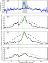 |
Fig. 4 Temporal evolution of the electron density and the line intensity. Panel a: the electron density in the source
region of OIV in the transition region derived from the ratio of the intercombination O IV lines at 1401 and
1400 Å including an error estimate. The black solid curve shows the fit to the density variation. For this fit the
time range indicated by the shaded area was ignored because these data points are flawed by the strong blending
of O IV 1401 Å by the excess emission in the far blue wing of Si IV 1403 Å. Panels b to d: the normalized intensity
|


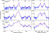 |
Fig. 5 Detailed look at the line profiles of O IV 1400 and 1401 Å, Si IV 1402 Å, and C II 1335 and 1336 Å before the event (top), at thefirst maximum brightening (middle), and the second maximum brightening (bottom). The red lines show the modified profiles of Si IV 1394 Å, which are shifted in wavelength and scaled in intensity to roughly match the target lines (Si IV 1402 Å, O IV 1400 and 1401 Å, and C II 1335 and 1336 Å). These are shown for a better comparison of the profiles of the different lines. The wavelengths are given in Doppler-shift units relative to the rest wavelength of Si IV 1403 Å and C II 1335 Å. We do not overplot the Si IV 1394 Å profile on O IV 1401 Å at 09:34:25 UT because of the strong blend by the blue wing of Si IV 1402 Å. See Sect. 4. |
5 Flows and structure in and below the loop
5.1 Spectroscopic properties
To investigate the flow structure at the location of the brightening, we investigated the line profile of Si IV in detail. Here we found several clearspectral components in the blue and in the red wing, indicating upward and downward motions along the LOS. This is the case mainly during the phase 2 of the brightening, and it applies to the Si IV 1394 Å and 1403 Å lines. Because thetwo Si IV lines are very similar, we only display the profile of Si IV 1394 Å in Fig. 6.
The Si IV profiles show three distinct components with changing Doppler shift in time, indicating a change in flow speed. In Fig. 6 we overplot a by-eye Gaussian fit on the spectra to highlight these distinct components (blue, green, and red profile).
The clearest and fastest flow component is in the far blue wing (blue Gaussian profiles in Fig. 6). As time progresses (from bottom to top), the Doppler shift of this component changes from ~ − 70 km s−1 (at 114 s) to ~ −265 km s−1 (at 141 s). This evolution of the spectral component in the blue wing suggests an accelerating upflow that reaches ~265 km s−1, which would be well above the sound speed and more comparable to the local Alfvén speed (depending on the assumption for the magnetic field). If this is indeed an accelerating upflow, it would travel ~5 Mm in total.
In addition to this most prominent upflow component, a slower upflow component is also visible, with a Doppler speed slower than 100 km s−1. This is highlighted with black arrows in Fig. 6. The slow upflow component starts later than the fast flow component. These observations of multiple upflow components suggest that there might be some activities, magnetic reconnection, for instance, that occur below the loop and launch the upflows.
In addition to the blueshifted components, a clear red component is visible (red Gaussian in Fig. 6). It appears after the high-speed upflow reaches a speed of more than ~200 km s−1, only seconds before the high-speed upflow ceases. The redshifted component is decelerated from about +160 km s−1 (at 136 s) to +120 km s−1 (at 151 s). This red component might be interpreted as the rebound flow of the upflow after it is stopped by an above-lying obstacle, which might be the overarching cool loop (see Sect. 6).
Throughout this event, we see a clear self-reversal of the Si IV line in all the spectra shown in Fig. 6. This self-reversion is visible not only in the 1394 Å line shown here, but also in the 1403 Å line of Si IV. This is similar to the spectra presented by Yan et al. (2015), who first reported such self-reversals of a transition region line.
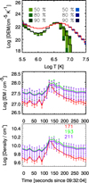 |
Fig. 6 Upper panel: the estimated DEM from six AIA EUV channels (171 Å, 193 Å, 211 Å, 131 Å, 335 Å, and 94 Å)
around 09:33:37 UT (at 93 s, black profile with green error bars) and 09:34:25 UT (at 141 s, red profile with blue error
bars) at theregion indicated with the red rectangles in Fig. 2. The colors from light to dark correspond
to the confidence interval with a confidence level of 50%, 80%, and 90%, respectively. Middle panel: the emission
measure of the 171 Å, 193 Å, and 211 Å channels obtained by integrating the DEM profile over the temperature range of
105.7 − 106.1 K,
106.05 − 106.3 K,
and 106.15−106.35 K,
respectively. The error bars are estimated from the confidence interval with a confidence level of
90%.
Lower panel:the electron density estimated by |
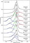 |
Fig. 7 Line profiles of Si IV 1394 Å during phase 2 of the brightening. These are stacked profiles, i.e., each time step is plotted with an intensity increased by 500 counts. These profiles are taken in the middle of the loop crossing the slit (see arrow in bottom left panel of Fig. 2). The colored Gaussian profiles indicate by-eye fits to the obvious spectral features in the line wings. Each set of the blue, green, and red profiles has the same width. The blue profiles are shifted by −70 km s−1 , −115 km s−1, −230 km s−1 , −250 km s−1 , −255 km s−1 , and −265 km s−1 , from bottom to top. The center of each blue Gaussian is marked by a black bar. The green profiles show the possible blueshifted components with lower speed, while the red profiles highlight a redshifted component. See Sect. 5.1. |
5.2 Relation to the magnetic field
To understand the cause of the accelerating upflow discussed in Sect. 5.1, we investigated the structure and evolution of the magnetic field at the solar surface below this brightening. For this we studied the LOS photospheric magnetic field from the HMI.
The middle part of the loop that shows the strong brightening is located above a mixed-polarity region between two sunspots (top panel in Fig. 8; the spectra discussed in Sect. 5.1 are located at the center of the red cross). Around the region of interest, the total magnetic flux shows a significant increase followed by a decrease (middle panel in Fig. 8). This is a clear indication that new magnetic flux emerges below the loop we investigate here before t = 0. When the magnetic flux fully emerges and begins to peter out, the rise in intensity of Si IV becomes significant. There might be a delay between the increase in Si IV with respect to the magnetic flux variation, which can be attributed to the Alfvén crossing time for the magnetic perturbation traveling from the photosphere to the Si IV source region. To estimate the Alfvén crossing time, we assumed a chromospheric Alfvén speed of V A ≈ 10 km s−1 (e.g., Hollweg 1978, 1981). The distance from the photosphere to the Si IV source region is roughly 2–3 Mm, therefore the Alfvén crossing time is 200–300 s. Here we assumed τA ≈ 250 s. When we consider the Alfvén crossing time, the intensity increase of Si IV is consistent with the flux increase, that is, with the emergence of the magnetic flux. The increased emission of Si IV might be due to heating related to reconnection during the emergence and/or the cancelation of the magnetic flux.
To investigate the magnetic topology near the loop apex, we employed a linear force-free field extrapolation (e.g., Seehafer 1978; Wiegelmann 2004; He et al. 2007) to the photospheric LOS magnetic field as obtained from the HMI. The extrapolated magnetic field lines near the loop apex show the signature of a dip in the middle part (marked in green in Fig. 9). Together with the appearance of the high-speed upflows, this magnetic field configuration indicates that there might be magnetic reconnection between the small-scale flux tubes (marked in blue in Fig. 9). This suggests that the heating of the cool loop is probably due to magnetic reconnection between the small-scale loops below the loop apex.
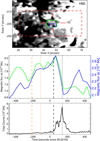 |
Fig. 8 Evolution of the magnetic flux below the loop apex and the total intensity of Si IV 1394 Å. Top panel: the magnetogram obtained by the HMI at 09:34:40 UT. The red dashed rectangle shows the field of view of Fig. 2. The red horizontal and vertical lines that form a cross indicate the location of the loop apex at the slit position. The green and blue rectangles indicate the region from which the total magnetic flux is obtained. Middle panel: the evolution of the total magnetic flux in the regions shown by green and blue rectangles in the top panel. Bottom panel: the evolution of the total intensity in Si IV 1394 Å. The black dashed and dotted lines show the onset of the brightening and the maximum brightening, respectively. The brown dashed and dotted lines show the corresponding time of the onset and maximum brightening subtracted by the Alfvén crossing time. See Sect. 5.2. |
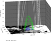 |
Fig. 9 Extrapolated 3D magnetic field lines overplotted on the photosheric magnetogram. Blue lines show the small-scale magnetic flux tubes connected to the small bipole region indicated with the blue rectangle in Fig. 8. Green lines indicate the magnetic field lines that show a dip near their middle part. White lines indicate the overlying large-scale loop. White lines are closed lines, only part of the lines is shown here in order to highlight the small-scale flux tubes. See Sect. 5.2. |
6 Discussion
Here we reported the singular case of a loop that was heated (from below) near the apex. The loop is visible in 1600 Å and invisible in 1700 Å, indicating that the signature in 1600 Å is due to transition region emission (the C IV doublet at 1548 Å and 1550 Å). The loop experienced two main phases of brightening. In phase 1, the temperature of the loop was relatively low and constrained to below a few 105 K. In phase 2, the appearance of almost the full loop in the 0.7 to 2 MK channels and in even hotter channels of AIA indicates that the loop was hotter than in phase 1.
In the second phase, a possible accelerating upflow whose Doppler velocity was shifted continuously from ~ − 70 km s−1 to ~ − 265 km s−1, was identified in the line profile of the two Si IV lines. The possible upflowing plasma roughly travels a distance of ~5 Mm. This strong upflow is associated with the appearance of the loop in the 0.7 to 2 MK channels and in even hotter channels of AIA. It is probably related to a magnetic flux emergence and the succeeding cancellation in the photosphere just below the loop apex. The extrapolated 3D magnetic field lines shows possible signatures of magnetic reconnection between two small-scale flux tubes below the loop apex, suggesting that the heating of the loop is probably due to the interaction between the overlying loop and the outflow from the magnetic reconnection between two small-scale flux tubes.
Except for the possible heating phase, in which the estimated electron density is not reliable, the relation between the intensity and density is consistent with the scenario that the intensity variation is mainly governed by the density variation, that is, the intensity variation of the optically thin line Si IV is consistent with the variation of the density squared and the intensity variation of the optically thick line C II is consistent with the density variation. The intensity variation of the optically thin line O IV 1400 Å is not fully consistent with that of the density squared owing to the intercombination line nature of O IV 1400 Å, whose emission may be suppressed by collision deexcitation that is due to the density enhancement. These results suggest that plasma fills the loop, which might be due to the compression or other processes.
During the loop brightening, the Si IV lines behave quite differently from O IV (middle and bottom panels in Fig. 5). The strong enhancement in the wings of the Si IV lines is not visible in O IV. We see at least three possible explanations: (1) the temperature of the plasma in the source region of the Si IVwings could be lower than the formation temperatureof O IV; (2) the density is so high that the intercombination lines of O IV are no longer visible, just like in the scenario described by Peter et al. (2014); (3) finally, the distribution function of the exciting electrons has an excess of high-energy electrons, which would also reduce the emission in the intercombination lines (cf. Dudík et al. 2014).
Based on our observations, we draw the following scenario (cf. Fig. 10). First there is a cool loop connecting the main polarities in the active region (uppermost field lines stretching from the far left to the right in Fig. 10). Between themain polarities of the active region, a small bipolar region then emerges that connects to the adjacent opposite-polarity region. This bipolar region shows an emerging and ceasing magnetic flux. While the flux emerges and ceases, some reconnection occurs that drives the fast upflow. This fast upflow occurs below the preexisting cool loop that causes self-absorption in the Si IV line (Yan et al. 2015). The fast upward flow of plasma then hits the overlying loop and significantly heats the envelope loop, which is therefore visible in the hot channels of AIA. After the strong upflow hits the overlying loop, the flow is in part reflected, causing the enhancement in the red wing of the Si IV line. When the upflow hits the overlying loop, two lateral flows would occur along the overlying loop. However, the lateral flows were not observed in this case owing to the sit-and-stare mode of the spectroscopic observation. This observational scenario is consistent with the previous numerical models of the emergence of magnetic fields (e.g., Syntelis et al. 2015; Archontis et al. 2007).
This scenario is probably too simple to truly catch the processes that underlie this observation. It still emphasizes that even a comparably simple loop, which might be considered to be well described by a 1D picture, might be more complex than thought initially. At least in the present case, where the brightening appeared at the apex, there is ample evidence that we need to consider thefull 3D nature of the atmosphere to describe this loop, which appeared to be 1D in the imaging observations. In this case, spectroscopy adds information that requires us to recognize the complexity of the solar atmosphere.
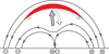 |
Fig. 10 Scenario for the event. The black lines indicate magnetic field lines, the plus and minus within an empty circle denote opposite magnetic polarities. The red cross shows a possible reconnection site between the small-scale magnetic flux tubes. The arrows indicate the flow patterns, and the red region represents the hot plasma that is heated near the loop apex by the interaction of the upflow with the above-lying magnetic loop. The gray solid arrow and the black dashed arrow stand for the upflow and possible rebound flow. The green arrows show the possible two lateral flows that have not been observed in this case, probably owing to the sit-and-stare mode of the spectral observation. See Sect. 6. |
Movie
Movie of Fig. 2 Access Supplementary Material
Acknowledgements
IRIS is a NASA Small Explorer mission developed and operated by LMSAL, with mission operations executed at NASA Ames Research Center and major contributions to downlink communications funded by the Norwegian Space Centre through a European Space Agency PRODEX contract. The Solar Dynamics Observatory (SDO) data that we used are provided courtesy of NASA/SDO and the Atmospheric Imaging Assembly and Helioseismic and Magnetic Imager science teams. The authorsthank the anonymous referee for suggestions. We thank Y. Chen, Z.J. Ning, Y. Li, and L.P. Yang for valuable discussions. The work at Peking University is supported by NSFC under contracts 41574168, 41231069, 41274172, 41474148, 41421003. LM Yan is supported by National Postdoctoral Program for Innovative Talents (grant BX201600159). J.S. H.E. is also supported by “National Youth Talent Support Program” of China. L.D. Xia is supported by NSFC under contracts 41274178 and 41474150.
Appendix A Additional table
Appendix B Estimating the electron density from IRIS spectral observations
We used theratio of the intercombination lines of O IV at 1401 Å and 1400 Å to estimate the electron density. To obtain the line ratio of the two O IV lines, we first estimated the total intensity of each O IV line after subtracting the continuum level.
When the O IV 1401 Å was heavily blended by the far blue wing of Si IV 1403 Å, we estimated the total intensity of O IV 1401 Å after subtracting the contribution of the wing of Si IV 1403 Å. This was done by using the (scaled and shifted) profile of Si IV 1394 Å.However, this process seems to overcorrect (oversubtract) the O IV line at 1401 Å when there is strong blending by the far wingof Si IV. This then leads to a too weak intensity of O IV 1401 Å and consequently to an underestimation of the line ratio and an overestimation of the electron density. In Fig. B.1 we show the line profile of the two O IV lines at four time steps, 09:32:04 UT (before the event), 09:33:07 UT (in phase 1), 09:34:25 UT (when the OIV 1401 Å is heavily blended by Si IV 1403 Å), and 09:35:21 UT (after the event) to illustrate this problem.
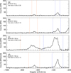 |
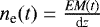
Fig. B.1 Spectral range around the intercombination O IV lines to estimate the electron density. The Si IV line is not part of this range and would peak around a Doppler shift of 0 km s−1 . The orange and blue lines show the Doppler-shift range we used to estimate the total intensity of O IV 1400 Å and the total intensity of O IV 1401 Å, respectively. The black dashed horizontal lines show the continuum level. |
Based on the theoretical relation between the line ratio and electron density obtained from the Chianti database (Landi et al. 2013), the electron density was estimated from the line ratio of O IV 1401 Å and 1400 Å (see Fig. B.2). The estimated electron density is reliable only when the line ratio is in the range between ~ 2.6 and ~ 5.5. The estimation of the electron density at the four time frames above is overplotted in Fig. B.2. by dots (with bars for the error estimates). The line ratio estimated at 09:34:25 UT is ~ 2.26 and thus too low to obtain a reliable electron density. We can therefore only set an upper limit on the electron density of 1013 cm−3.
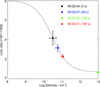 |
Fig. B.2 Example for the estimation of the electron density at the source region of O IV. The black solid curve shows the theoretical relation between the electron density and the line ratio of O IV 1401 Å and O IV 1400 Å obtained from the Chianti database. The colored dots show the line ratio and density for the four sample spectra in Fig. B.1. The horizontal and vertical bars show the uncertainty of the estimated electron density. |
References
- Archontis, V., Hood, A. W., & Brady, C. 2007, A&A, 466, 367 [NASA ADS] [CrossRef] [EDP Sciences] [Google Scholar]
- Aschwanden, M. J., Schrijver, C. J., & Alexander, D. 2001, ApJ, 550, 1036 [NASA ADS] [CrossRef] [Google Scholar]
- Aschwanden, M. J., Winebarger, A., Tsiklauri, D., & Peter, H. 2007, ApJ, 659, 1673 [NASA ADS] [CrossRef] [Google Scholar]
- Athay, R. G. 1966, ApJ, 146, 223 [NASA ADS] [CrossRef] [Google Scholar]
- Bingert, S., & Peter, H. 2011, A&A, 530, A112 [NASA ADS] [CrossRef] [EDP Sciences] [Google Scholar]
- Boerner, P., Edwards, C., Lemen, J., et al. 2012, Sol. Phys., 275, 41 [NASA ADS] [CrossRef] [Google Scholar]
- Buchlin, E., Cargill, P. J., Bradshaw, S. J., & Velli, M. 2007, A&A, 469, 347 [NASA ADS] [CrossRef] [EDP Sciences] [Google Scholar]
- Carlsson, M., & Leenaarts, J. 2012, A&A, 539, A39 [NASA ADS] [CrossRef] [EDP Sciences] [Google Scholar]
- Chen, F., Peter, H., Bingert, S., & Cheung, M. C. M. 2014, A&A, 564, A12 [NASA ADS] [CrossRef] [EDP Sciences] [Google Scholar]
- Cheng, X., Zhang, J., Saar, S. H., & Ding, M. D. 2012, ApJ, 761, 62 [NASA ADS] [CrossRef] [Google Scholar]
- Cheung, M. C. M., Boerner, P., Schrijver, C. J., et al. 2015, ApJ, 807, 143 [NASA ADS] [CrossRef] [Google Scholar]
- Chiuderi, C., Einaudi, G., & Torricelli-Ciamponi, G. 1981, A&A, 97, 27 [NASA ADS] [Google Scholar]
- De Pontieu, B., Title, A. M., Lemen, J. R., et al. 2014, Sol. Phys., 289, 2733 [NASA ADS] [CrossRef] [Google Scholar]
- Dudík, J., Del Zanna, G., Dzifčáková, E., Mason, H. E., & Golub, L. 2014, ApJ, 780, L12 [NASA ADS] [CrossRef] [Google Scholar]
- Gudiksen, B. V., & Nordlund, Å. 2002, ApJ, 572, L113 [Google Scholar]
- Hansteen, V. H., Hara, H., De Pontieu, B., & Carlsson, M. 2010, ApJ, 718, 1070 [Google Scholar]
- He, J.-S., Tu, C.-Y., & Marsch, E. 2007, A&A, 468, 307 [NASA ADS] [CrossRef] [EDP Sciences] [Google Scholar]
- Hollweg, J. V. 1978, Sol. Phys., 56, 305 [NASA ADS] [CrossRef] [Google Scholar]
- Hollweg, J. V. 1981, Sol. Phys., 70, 25 [NASA ADS] [CrossRef] [Google Scholar]
- Kano, R., & Tsuneta, S. 1996, PASJ, 48, 535 [NASA ADS] [CrossRef] [Google Scholar]
- Klimchuk, J. A. 2006, Sol. Phys., 234, 41 [NASA ADS] [CrossRef] [Google Scholar]
- Landi, E., Young, P. R., Dere, K. P., Del Zanna, G., & Mason, H. E. 2013, ApJ, 763, 86 [NASA ADS] [CrossRef] [Google Scholar]
- Lemen, J. R., Title, A. M., Akin, D. J., et al. 2012, Sol. Phys., 275, 17 [NASA ADS] [CrossRef] [Google Scholar]
- Li, L. P., Peter, H., Chen, F., & Zhang, J. 2015, A&A, 583, A109 [NASA ADS] [CrossRef] [EDP Sciences] [Google Scholar]
- Mariska, J. T. 1992, The Solar Transition Region (Cambridge: Cambridge Univ. Press) [Google Scholar]
- Matsumoto, T., & Suzuki, T. K. 2014, MNRAS, 440, 971 [NASA ADS] [CrossRef] [Google Scholar]
- Nagai, F. 1980, Sol. Phys., 68, 351 [NASA ADS] [CrossRef] [Google Scholar]
- Peter, H. 2015, Philos. Trans. Roy. Soc. Lond. Ser. A, 373, 20150055 [Google Scholar]
- Peter, H., Tian, H., Curdt, W., et al. 2014, Science, 346, C315 [NASA ADS] [CrossRef] [Google Scholar]
- Priest, E. R., Foley, C. R., Heyvaerts, J., et al. 1998, Nature, 393, 545 [NASA ADS] [CrossRef] [Google Scholar]
- Priest, E. R., Foley, C. R., Heyvaerts, J., et al. 2000, ApJ, 539, 1002 [NASA ADS] [CrossRef] [Google Scholar]
- Reale, F. 2002, ApJ, 580, 566 [NASA ADS] [CrossRef] [Google Scholar]
- Reale, F. 2014, Liv. Rev. Sol. Phys., 11, 4 [Google Scholar]
- Rosner, R., Tucker, W. H., & Vaiana, G. S. 1978, ApJ, 220, 643 [NASA ADS] [CrossRef] [Google Scholar]
- Schmelz, J. T., Kimble, J. A., Jenkins, B. S., et al. 2010, ApJ, 725, L34 [NASA ADS] [CrossRef] [Google Scholar]
- Schmelz, J. T., Rightmire, L. A., Saar, S. H., et al. 2011a, ApJ, 738, 146 [NASA ADS] [CrossRef] [Google Scholar]
- Schmelz, J. T., Worley, B. T., Anderson, D. J., et al. 2011b, ApJ, 739, 33 [NASA ADS] [CrossRef] [Google Scholar]
- Schou, J., Scherrer, P. H., Bush, R. I., et al. 2012, Sol. Phys., 275, 229 [Google Scholar]
- Seehafer, N. 1978, Sol. Phys., 58, 215 [NASA ADS] [CrossRef] [Google Scholar]
- Syntelis, P., Archontis, V., Gontikakis, C., & Tsinganos, K. 2015, A&A, 584, A10 [NASA ADS] [CrossRef] [EDP Sciences] [Google Scholar]
- Ugarte-Urra, I., & Warren, H. P. 2014, ApJ, 783, 12 [NASA ADS] [CrossRef] [Google Scholar]
- van Wettum, T., Bingert, S., & Peter, H. 2013, A&A, 554, A39 [NASA ADS] [CrossRef] [EDP Sciences] [Google Scholar]
- Vernazza, J. E., Avrett, E. H., & Loeser, R. 1981, ApJS, 45, 635 [NASA ADS] [CrossRef] [Google Scholar]
- Warren, H. P., Winebarger, A. R., & Brooks, D. H. 2012, ApJ, 759, 141 [NASA ADS] [CrossRef] [Google Scholar]
- Wiegelmann, T. 2004, Sol. Phys., 219, 87 [NASA ADS] [CrossRef] [Google Scholar]
- Winebarger, A. R., Schmelz, J. T., Warren, H. P., Saar, S. H., & Kashyap, V. L. 2011, ApJ, 740, 2 [NASA ADS] [CrossRef] [Google Scholar]
- Yan, L., Peter, H., He, J., et al. 2015, ApJ, 811, 48 [NASA ADS] [CrossRef] [Google Scholar]
Part of the SolarSoft package, http://www.lmsal.com/solarsoft/
All Tables
All Figures
|
Fig. 1 Context of the active region as seen in AIA 193 Å, showing plasma around 1.5 MK. The FOV is 249.6″ × 249.6″ centered at solar X = 50″ and solar Y = −225″. The white dashed and solid rectangles indicate the full FOV of IRIS and the subregion shown in Fig. 2, respectively.See Sect. 2. |
| In the text | |
|
Fig. 2 Temporal evolution of the loop. The four rows show snapshots at the indicated times. The columns show the images obtained through the IRIS slit-jaw-images in 1400 Å, the AIA channels at 171 Å and 193 Å, and the Fe xviii (93.92 Å) emission extracted from the AIA channel at 94 Å. The images show plasma at increasing temperatures at below 0.1 MK, 1 MK, 1.5 MK, and at around 7 MK. The black dashed vertical lines indicate the slit position of the IRIS spectrometer. Red arrows point at the loop studied here. Red rectangles show the region of the differential emission measure (DEM) analysis, the result of which is shown in Fig. 7. The color tables shows the data number per pixel on a log 10 scale. The same color table is used for each wavelength channel at the different time steps. The field of view is indicated in Fig. 1 by the solid rectangle. See Sect. 3. A corresponding animation, Animation 1, is available in the online journal. |
| In the text | |
|
Fig. 3 Temporal evolution of the line profiles of Si IV, O IV, and C II. The three rows show spectral windows centered around Si IV 1394 Å (top), Si IV 1403 Å, including the nearby inter-combination lines of O IV (middle), and C II 1335 Å and 1336 Å (bottom). The wavelengths are given in Doppler-shift units relative to the rest wavelengths of Si IV 1394 Å, Si IV 1403 Å, andC II 1336 Å. Each panel shows the time evolution of the line profiles over 3.5 min starting at 09:32:40 UT. Different line colors represent different times, as indicated by the color bar showing the time in seconds since 09:32:04 UT. All spectra are taken at the location along the slit in the middle of the loop crossing the slit (see the arrow in the lower left panel of Fig. 2). See Sect. 3. |
| In the text | |
|
Fig. 4 Temporal evolution of the electron density and the line intensity. Panel a: the electron density in the source
region of OIV in the transition region derived from the ratio of the intercombination O IV lines at 1401 and
1400 Å including an error estimate. The black solid curve shows the fit to the density variation. For this fit the
time range indicated by the shaded area was ignored because these data points are flawed by the strong blending
of O IV 1401 Å by the excess emission in the far blue wing of Si IV 1403 Å. Panels b to d: the normalized intensity
|
| In the text | |
|
Fig. 5 Detailed look at the line profiles of O IV 1400 and 1401 Å, Si IV 1402 Å, and C II 1335 and 1336 Å before the event (top), at thefirst maximum brightening (middle), and the second maximum brightening (bottom). The red lines show the modified profiles of Si IV 1394 Å, which are shifted in wavelength and scaled in intensity to roughly match the target lines (Si IV 1402 Å, O IV 1400 and 1401 Å, and C II 1335 and 1336 Å). These are shown for a better comparison of the profiles of the different lines. The wavelengths are given in Doppler-shift units relative to the rest wavelength of Si IV 1403 Å and C II 1335 Å. We do not overplot the Si IV 1394 Å profile on O IV 1401 Å at 09:34:25 UT because of the strong blend by the blue wing of Si IV 1402 Å. See Sect. 4. |
| In the text | |
|
Fig. 6 Upper panel: the estimated DEM from six AIA EUV channels (171 Å, 193 Å, 211 Å, 131 Å, 335 Å, and 94 Å)
around 09:33:37 UT (at 93 s, black profile with green error bars) and 09:34:25 UT (at 141 s, red profile with blue error
bars) at theregion indicated with the red rectangles in Fig. 2. The colors from light to dark correspond
to the confidence interval with a confidence level of 50%, 80%, and 90%, respectively. Middle panel: the emission
measure of the 171 Å, 193 Å, and 211 Å channels obtained by integrating the DEM profile over the temperature range of
105.7 − 106.1 K,
106.05 − 106.3 K,
and 106.15−106.35 K,
respectively. The error bars are estimated from the confidence interval with a confidence level of
90%.
Lower panel:the electron density estimated by |
| In the text | |
|
Fig. 7 Line profiles of Si IV 1394 Å during phase 2 of the brightening. These are stacked profiles, i.e., each time step is plotted with an intensity increased by 500 counts. These profiles are taken in the middle of the loop crossing the slit (see arrow in bottom left panel of Fig. 2). The colored Gaussian profiles indicate by-eye fits to the obvious spectral features in the line wings. Each set of the blue, green, and red profiles has the same width. The blue profiles are shifted by −70 km s−1 , −115 km s−1, −230 km s−1 , −250 km s−1 , −255 km s−1 , and −265 km s−1 , from bottom to top. The center of each blue Gaussian is marked by a black bar. The green profiles show the possible blueshifted components with lower speed, while the red profiles highlight a redshifted component. See Sect. 5.1. |
| In the text | |
|
Fig. 8 Evolution of the magnetic flux below the loop apex and the total intensity of Si IV 1394 Å. Top panel: the magnetogram obtained by the HMI at 09:34:40 UT. The red dashed rectangle shows the field of view of Fig. 2. The red horizontal and vertical lines that form a cross indicate the location of the loop apex at the slit position. The green and blue rectangles indicate the region from which the total magnetic flux is obtained. Middle panel: the evolution of the total magnetic flux in the regions shown by green and blue rectangles in the top panel. Bottom panel: the evolution of the total intensity in Si IV 1394 Å. The black dashed and dotted lines show the onset of the brightening and the maximum brightening, respectively. The brown dashed and dotted lines show the corresponding time of the onset and maximum brightening subtracted by the Alfvén crossing time. See Sect. 5.2. |
| In the text | |
|
Fig. 9 Extrapolated 3D magnetic field lines overplotted on the photosheric magnetogram. Blue lines show the small-scale magnetic flux tubes connected to the small bipole region indicated with the blue rectangle in Fig. 8. Green lines indicate the magnetic field lines that show a dip near their middle part. White lines indicate the overlying large-scale loop. White lines are closed lines, only part of the lines is shown here in order to highlight the small-scale flux tubes. See Sect. 5.2. |
| In the text | |
|
Fig. 10 Scenario for the event. The black lines indicate magnetic field lines, the plus and minus within an empty circle denote opposite magnetic polarities. The red cross shows a possible reconnection site between the small-scale magnetic flux tubes. The arrows indicate the flow patterns, and the red region represents the hot plasma that is heated near the loop apex by the interaction of the upflow with the above-lying magnetic loop. The gray solid arrow and the black dashed arrow stand for the upflow and possible rebound flow. The green arrows show the possible two lateral flows that have not been observed in this case, probably owing to the sit-and-stare mode of the spectral observation. See Sect. 6. |
| In the text | |
|
Fig. B.1 Spectral range around the intercombination O IV lines to estimate the electron density. The Si IV line is not part of this range and would peak around a Doppler shift of 0 km s−1 . The orange and blue lines show the Doppler-shift range we used to estimate the total intensity of O IV 1400 Å and the total intensity of O IV 1401 Å, respectively. The black dashed horizontal lines show the continuum level. |
| In the text | |
|
Fig. B.2 Example for the estimation of the electron density at the source region of O IV. The black solid curve shows the theoretical relation between the electron density and the line ratio of O IV 1401 Å and O IV 1400 Å obtained from the Chianti database. The colored dots show the line ratio and density for the four sample spectra in Fig. B.1. The horizontal and vertical bars show the uncertainty of the estimated electron density. |
| In the text | |
Current usage metrics show cumulative count of Article Views (full-text article views including HTML views, PDF and ePub downloads, according to the available data) and Abstracts Views on Vision4Press platform.
Data correspond to usage on the plateform after 2015. The current usage metrics is available 48-96 hours after online publication and is updated daily on week days.
Initial download of the metrics may take a while.