| Issue |
A&A
Volume 610, February 2018
|
|
|---|---|---|
| Article Number | A32 | |
| Number of page(s) | 20 | |
| Section | Extragalactic astronomy | |
| DOI | https://doi.org/10.1051/0004-6361/201731952 | |
| Published online | 22 February 2018 | |
VLBA polarimetric monitoring of 3C 111
1
Dr. Remeis-Sternwarte & Erlangen Centre for Astroparticle Physics, Universität Erlangen-Nürnberg,
Sternwartstrasse 7,
96049
Bamberg,
Germany
e-mail: This email address is being protected from spambots. You need JavaScript enabled to view it.
2
Lehrstuhl für Astronomie, Universität Würzburg,
Emil-Fischer-Str. 31,
97074
Würzburg,
Germany
3
Departament d’Astronomia i Astrofísica, Universitat de València C/ Dr. Moliner 50,
46100
Burjassot,
València,
Spain
4
Observatori Astronòmic, Universitat de València, Parc Científic, C. Catedrático José Beltrán 2,
46980
Paterna,
València,
Spain
5
Max-Planck-Institut für extraterrestrische Physik (MPE),
PO 1312,
85741
Garching,
Germany
6
Netherlands Institute for Radio Astronomy (ASTRON),
PO Box 2,
7990 AA
Dwingeloo,
The Netherlands
7
Instituto de Astrofísica de Andalucía-CSIC,
Apartado 3004,
18080
Granada,
Spain
8
Max-Planck-Institut für Radioastronomie,
Auf dem Hügel 69,
53121
Bonn,
Germany
9
Harvard-Smithsonian Center for Astrophysics,
60 Garden St.,
Cambridge,
MA
02138,
USA
10
Department of Physics, Denison University,
100 W College St.,
Granville,
OH
43023,
USA
11
Astro Space Center of Lebedev Physical Institute,
Profsoyuznaya 84/32,
117997
Moscow,
Russia
12
Moscow Institute of Physics and Technology, Dolgoprudny,
Institutsky per., 9,
141700
Moscow region,
Russia
13
Department of Physics and Astronomy, Purdue University,
525 Northwestern Avenue,
West Lafayette,
IN
47907,
USA
14
Anton Pannekoek Institute for Astronomy,
PO Box 94249,
1090 GE
Amsterdam,
The Netherlands
15
Crimean Astrophysical Observatory,
98409
Nauchny,
Crimea
16
Aalto University Department of Electronics and Nanoengineering, PL 15500,
00076
Aalto,
Finland
17
Aalto University Metsähovi Radio Observatory,
Metsähovintie 114,
02540
Kylmälä,
Finland
18
Instituto de Radio Astronomía Milimétrica, Avenida Divina Pastora,
7, Local 20,
18012
Granada,
Spain
Received:
14
September
2017
Accepted:
30
October
2017
Abstract
Context. While studies of large samples of jets of active galactic nuclei (AGN) are important in order to establish a global picture, dedicated single-source studies are an invaluable tool for probing crucial processes within jets on parsec scales. These processes involve in particular the formation and geometry of the jet magnetic field as well as the flow itself.
Aims. We aim to better understand the dynamics within relativistic magneto-hydrodynamical flows in the extreme environment and close vicinity of supermassive black holes.
Methods. We analyze the peculiar radio galaxy 3C 111, for which long-term polarimetric observations are available. We make use of the high spatial resolution of the VLBA network and the MOJAVE monitoring program, which provides high data quality also for single sources and allows us to study jet dynamics on parsec scales in full polarization with an evenly sampled time-domain. While electric vectors can probe the underlying magnetic field, other properties of the jet such as the variable (polarized) flux density, feature size, and brightness temperature, can give valuable insights into the flow itself. We complement the VLBA data with data from the IRAM 30-m Telescope as well as the SMA.
Results. We observe a complex evolution of the polarized jet. The electric vector position angles (EVPAs) of features traveling down the jet perform a large rotation of ≳180∘ across a distance of about 20 pc. As opposed to this smooth swing, the EVPAs are strongly variable within the first parsecs of the jet. We find an overall tendency towards transverse EVPAs across the jet with a local anomaly of aligned vectors in between. The polarized flux density increases rapidly at that distance and eventually saturates towards the outermost observable regions. The transverse extent of the flow suddenly decreases simultaneously to a jump in brightness temperature around where we observe the EVPAs to turn into alignment with the jet flow. Also the gradient of the feature size and particle density with distance steepens significantly at that region.
Conclusions. We interpret the propagating polarized features as shocks and the observed local anomalies as the interaction of these shocks with a localized recollimation shock of the underlying flow. Together with a sheared magnetic field, this shock-shock interaction can explain the large rotation of the EVPA. The superimposed variability of the EVPAs close to the core is likely related to a clumpy Faraday screen, which also contributes significantly to the observed EVPA rotation in that region.
Key words: galaxies: active / galaxies: jets / galaxies: individual: 3C 111 / galaxies: magnetic fields / radio continuum: galaxies / polarization
Now at Anton Pannekoek Institute for Astronomy, PO Box 94249, 1090 GE Amsterdam, The Netherlands.
© ESO 2018
1 Introduction
Collimated jet outflows have been observed in many active galactic nuclei (AGN). They may either be launched by magneto-centrifugal forces (Blandford & Payne 1982), by the extraction of energy from a Kerr black hole (Blandford & Znajek 1977), or by a combination of both. Both predict increasing magnetization of the produced jet towards the black hole. Modern GRMHD simulations extend on these formalisms and turn out to be good descriptions of observed jets (e.g., McKinney & Gammie 2004; Tchekhovskoy et al. 2011).
Such jets have been shown to be strong emitters across the electromagnetic spectrum (e.g., Clautice et al. 2016, for the kpc-scale jet of 3C 111). In the radio band, the technique of VLBI can resolve jets on parsec scales. In blazars, distinct features are typically found to be ejected at apparent superluminal velocities (e.g., Lister et al. 2013) and emit a non-thermal synchrotron spectrum, reflecting the presence of relativistic charged particles in a magnetic field that is at least partially ordered at the location of these features.
Polarization sensitive observations of parsec-scale jets have confirmed this notion and found many of these features to be significantly polarized (e.g., Homan 2005). The degree of polarization typically lies around a few percent in the subparsec-scale core region and increases to higher levels in the jet further downstream, often coinciding with propagating features that are commonly interpreted as relativistic shocks (Königl 1981; Marscher & Gear 1985), which can enhance the total and polarized flux density. Polarimetry is therefore a valuable tool to also study the magnetic field structure inside jets. Studies of large samples of blazars seem to confirm a quasi-bimodal distribution of electric vector position angles (EVPAs) with the majority of VLBI knots in BL Lac objects showing aligned EVPAs, while this picture is not as clear for quasars (Gabuzda et al. 1994, 2000; Lister & Smith 2000; Lister & Homan 2005; Pollack et al. 2003). Wardle (1998, 2013) and Homan (2005) emphasize a non-negligible fraction of oblique EVPA orientations, that is, “local anomalies” in quasar jets as opposed to clear bimodal distributions (Agudo et al. 2018b). For the simplified case of an underlying axisymmetric and helical magnetic field, these results would imply a dominance of toroidally dominated fields in the inner jet of BL Lac objects (Lyutikov et al. 2005), and a range of field directions in quasars, for example, due to oblique shocks (Marscher et al. 2002). At larger distances, this picture may change: FR II radio galaxies, the likely parent populations of quasars, in general tend to produce perpendicular EVPAs farther downstream (Bridle 1984; Cawthorne et al. 1993b; Bridle et al. 1994), favoring the interpretation with strong axial field components.
While surveys of the polarization properties are important for the bigger picture, dedicated studies of the dynamics of spatially resolved polarized parsec-scale jets are invaluable to gain more insight into the complex processes inherent to these systems. Steady-state (general relativistic) magnetohydrodynamical ((G,R)MHD) simulations predict the formation of recollimation shocks in overpressured jets (e.g., Gómez et al. 1997; Mimica et al. 2009; Roca-Sogorb et al. 2009; Fromm et al. 2016; Martí et al. 2016). Observations were able to confirm such recollimation shocks for BL Lac (Cohen et al. 2014; Gómez et al. 2016), CTA 102 (Fromm et al. 2013, 2016) and 3C 120 (León-Tavares et al. 2010; Agudo et al. 2012). Recollimation shocks have also been associated with stationary features observed in radio galaxies and blazars close to the radio core at millimeter wavelengths (Jorstad et al. 2001, 2005, 2013; Kellermann et al. 2004; Britzen et al. 2010).
The evidence for recollimations close to the radio core fits into the frame of an early paradigm of a “master” recollimation (Marscher 2006; Marscher et al. 2008, 2010) limiting the acceleration and collimation zone (Beskin et al. 1998; Beskin & Nokhrina 2006; Meier 2013). This paradigm goes back to work by Daly & Marscher (1988) and Impey & Neugebauer (1988), who show that the core at millimeter wavelengths may not only be the τ = 1 surface but a characteristic feature, coinciding with a standing shock.
Fromm et al. (2016) show for the case of CTA 102 that shocks propagating downstream will eventually interact with such a standing conical recollimation shock. As Cawthorne (2006) outlines, conical recollimation shocks themselves can reveal a characteristic structure of EVPAs, which matches observations of the core of the blazar S5 1803+784 (Cawthorne et al. 2013) as well as a downstream feature in 3C 120 (Agudo et al. 2012). The polarization signatures of shock-shock interactions are, however, unclear, and have not yet been consistently quantified.
Meanwhile, systematic observations of blazars and radio galaxies report smooth rotations of the EVPA with time (Agudo et al. 2018b). Sample studies of blazars at optical wavelengths (e.g., Blinov et al. 2016) show that the amplitude of the rotations is typically very large, reaching more than 180° on comparatively short time scales. Prominent examples are BL Lac (Marscher et al. 2008), PKS 1510−089 (Marscher et al. 2010), and 3C 279 (Larionov et al. 2008; Abdo et al. 2010; Kiehlmann et al. 2016). In the radio band, however, large rotations of more than 90° are rare (e.g., Aller et al. 2003) and only found in a few sources (e.g., Altschuler 1980; Aller et al. 1981; Homan et al. 2002; Myserlis et al. 2016, including BL Lac and PKS 1510−089). Marscher et al. (2010) explain the large EVPA swing in PKS 1510−089 in terms of a projected, geometrical rotation in the presence of an ordered, helical field observed at a shallow angle (Larionov et al. 2008; Nalewajko 2010). For the same source, Myserlis et al. (2016) also find consistency with transitions between an optically thin and thick state of the polarized ejecta. As Homan et al. (2002) show, the EVPA swings of the majority of the 12 selected blazars are overall limited by 90°, consistent with changes of the underlying magnetic field from toroidally dominated to poloidally dominated or vice versa. These observations demonstrate the ambiguity when attempting to interpret polarimetric data.
Here, we are studying the long-term evolution of the parsec-scale jet of the AGN of 3C 111 that shows particularly bright and highly polarized traveling features. Our immediate aim is to study the interaction of moving shocks with a stationary recollimation shock. 3C 111 (z ~ 0.048; Véron-Cetty & Véron 2010) is classified as a FR II radio galaxy (Sargent 1977). Its extended twin jet-structure (Linfield & Perley 1984; Leahy et al. 1997) is inclined with a PA of about 63°. Its radio core is exceptionally compact and bright. The parsec-scale jet reveals features that undergo apparent superluminal motion and appears as one-sided due to beamed emission (Jorstad et al. 2005; Kadler et al. 2008; Chatterjee et al. 2011). These blazar-like properties contrast the morphology on larger scales, which is reminiscent of a typical radio galaxy. Long-term VLBI monitoring at 15 GHz by MOJAVE1 reveals strong structural variability on parsec scales as it has been observed in total and polarized intensity by Kadler et al. (2008), hereafter K08, Großberger et al. (2012) and Lister et al. (2013). 3C 111 was also subject to monitoring with the VLBA at 43 GHz between 1998 and 2001 (Jorstad et al. 2005) and between 2004 and 2010 (Chatterjee et al. 2011). All these studies revealed individual ballistic components with apparent superluminal speeds of up to 6 c, most of which are significantly polarized.
At higher energies, however, multiwavelength studies (Chatterjee et al. 2011; Tombesi et al. 2012) reveal that the emission is more reminiscent of a Seyfert galaxy, which makes 3C 111 a unique source to study the disk-jet connection. Its broad-band spectral energy distribution (SED) shows double-humped emission up to GeV energies (Hartman et al. 2008, and Fig. 1 for a version that is compiled with radio, UV and X-ray data from within the time-interval considered in this paper). While the soft energy hump is consistent with synchrotron emission, the high-energy emission can be described with a power law resulting from thermal and/or non-thermal Comptonization in a compact corona (de Jong et al. 2012; Tombesi et al. 2013).
In the following, we study 36 MOJAVE epochs between 2007 and 2012, both in total and polarized intensity. This paper is structured as follows. In Sect. 2 we outline the observational techniques including single-dish instruments at millimeter wavelengths and VLBI data at 15 GHz. In Sect. 3 the results are described for the dynamics of the polarized parsec-scale jet, while Sect. 4 provides corresponding interpretations. A summary is presented in Sect. 5. Appendix A includes a discussion on the viewing angle and describes a toy model facilitating the interpretation on the complex processes taking place in the polarized parsec-scale jet of 3C 111. Appendix B complements the discussion with respect to the option of a helical field geometry threading the jet of 3C 111.
The mass of the central black hole (BH) has been derived to be  (Chatterjee et al. 2011). We use the latest cosmological parameters provided by the Planck Collaboration XIII (2016), that is, Ωm = 0.308, Ωλ = 0.692, and H0 = 67.8 km s−1 Mpc−1 and find a correspondence of 1 pc∕1 mas = 1.08.
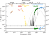 |
Fig. 1 Broad-band spectral energy distribution (SED) of 3C 111. The VLBA, IRAM, and SMA flux-density points are weighted averages over the time range probed in this paper (2007–2012). We show integrated core+jet flux densities from the VLBA and the SMA. The WISE (Wright et al. 2010) and 2MASS (Skrutskie et al. 2006) data are extracted from the All-Sky Source Catalog. The UV and X-ray data result from observations with Swift/UVOT and XRT (Burrows et al. 2005) on 2008-11-16. The hard X-ray INTEGRAL/IBIS/ISGRI spectrum has been obtained in the time-interval considered in this paper using the HEAVENS online tool (Walter et al. 2010). The black, solid curve represents a model of an incident power-law (upper dashed curve) that is being reprocessed in an accretion disk (lower dashed curve with prominent emission features). The residuals corresponding to the (hard) X-ray model are shown in the bottom panel. We can fit the XRT data well in combination with reflected emission from the accretion disk using xillver (García et al. 2013) and find χ (d.o.f.) = 47 (34). The statistics worsen when including the INTEGRAL data due to their scatter and systematic uncertainties that are not included here. |
2 Observations and data analysis
2.1 SMA
The 230 GHz and 350 GHz flux density data were obtained at the Submillimeter Array (SMA) near the summit of Mauna Kea (Hawaii). 3C 111 is included in an ongoing monitoring program at the SMA to determine flux densities of compact extragalactic radio sources that can be used as calibrators at millimeter wavelengths (Gurwell et al. 2007). Observations of available potential calibrators are from time to time observed for 3 to 5 min, and the measured source signal strength calibrated against known standards, typically solar system objects (Titan, Uranus, Neptune, or Callisto). Data from this program are updated regularly and are available at the SMA website2.
2.2 IRAM 30-m
We use data at 86 GHz and 230 GHz that were recorded with the correlation polarimeter XPOL (Thum et al. 2008) of the 30-m IRAM Telescope on Pico Veleta (Spain). Details on the instrumentation and observing technique are provided by Agudo et al. (2014). The data shown here are measured using the on-off technique with a wobbler of approximately 45′′. The data were taken in the framework of the POLAMI (Polarimetric Monitoring of AGN at Millimeter Wavelengths) program3 (Agudo et al. 2018a,b; Thum et al. 2018). The half-power beam widths are 28′′ and 11′′, respectively. The observations of the monitoring are spaced on the time-scale of weeks. In this paper we consider only data from mid 2010 until mid 2014.
2.3 MOJAVE
As part of the MOJAVE monitoring program, 3C 111 has been observed every few months at 15 GHz with the VLBA. K08 analyzed the first 17 epochs from 1995 to 2005. We are following up with the upcoming 36 epochs until mid-2012. The resulting interferometer visibilities were calibrated as described in Lister & Homan (2005). We desist from performing a detailed kinematic analysis and refer to Lister et al. (2013), Großberger (2014), and Homan et al. (2015) in that regard. The visibilities are naturally weighted and fitted in the (u, v)-plane using Gaussian model components. The fitted components are then interpreted with quasi-ballistical trajectories over as many epochs as possible. See Großberger (2014) for details.
We make use of the ModelFitPackage written for the Interactive Spectral Interpretation System (ISIS) (Houck & Denicola 2000; Großberger 2014). ISIS is designed for the spectral analysis of high-resolution X-ray data and provides a powerful and interactive tool for general astrophysical data analysis based on the S-Lang scripting language. Its programmability has turned ISIS into a tool well suited for fitting data of any kind. In particular, the isisscripts4 provide a pool of functions that are facilitating advanced data fitting and processing as well as analyzing astrophysical data in general. The ModelFitPackage interfaces between ISIS and difmap. In this way we are able to effectively explore the complex and multi-dimensional χ2 -space and to infer constraints on the model parameters. For a few prominent sources, Großberger (2014) calculates the statistical uncertainties for model component positions by probing the entire parameter space. When taking into account parameter degeneracies, we consider a conservative uncertainty of 0.05 mas. This value is consistent with the most probable uncertainty found by Lister et al. (2009), who analyze the deviations of the component positions from a common kinematic model and for the whole MOJAVE sample.
For deriving flux densities in the polarized channels Stokes Q and U, we use the total-intensity Gaussian model components provided by Großberger (2014). We freeze their positions and re-fit only the flux densities according to Lister & Homan (2005). This approach gives satisfactory results but we note that in extreme cases of rapid EVPA changes over core distance, the Q and U visibilities may not be properly approximated with Gaussian model components. We then calculate maps of linearly polarized intensity  and the EVPA = 0.5 arctan(U∕Q) for all 36 epochs treated in this publication. We show EVPAs uncorrected for Faraday rotation due to the lack of rotation measure (RM) information covering the entire parsec-scale jet as observed by MOJAVE. Similar to K08, we assume 15% uncertainties on the flux densities. In their Appendix, Homan et al. (2002) empirically derive distinct components to have flux uncertainties between 5% and 10% depending on the component strength. In our case, the uncertainties may be even higher due to relatively weak and closely spaced features, justifying the choice of 15%.
3 Revealing the polarized jet emission on pc scales
In recent years, 3C 111 showed three major outbursts, hereafter labeled A–C, starting in late 2005, 2007, and 2008, respectively. Figure 2 shows light curves taken by IRAM at 86 GHz and SMA at 230 GHz and 350 GHz. The most prominent outburst in late 2007 reached a maximum ≳13 Jy at 86 GHz, and the 2005 and 2008 outbursts reached only about half of that peak flux density. The outbursts can be associated with jet activity and the ejection of apparent superluminal components at 43 GHz (using archival data of the Boston University Blazar Group, hereafter BG5) and 15 GHz (MOJAVE). In the following, we study the evolution of the jet-plasma flow and its polarized emission on parsec scales.
3.1 Milliarcsecond-scale morphology and evolution
3.1.1 Image analysis
Figure 3 shows the evolution of the jet’s linearly polarized intensity as well as the EVPAs on top of the total intensity contours at 15 GHz as a result of MOJAVE (VLBA) observations. The images cover the range from 2007-01-06 through 2012-05-24 and are disjunct from the 1999–2006 period studied by K08. They reveal a number of distinct polarized patterns that can be described by a comparatively small number of model components close to the core and become increasingly complex further downstream. The polarized patterns are spatially coincident with features in total intensity that are propagating downstream. They originate from the most upstream stationary feature, the 15 GHz core that is mainly unpolarized. In the bottom panel of Fig. 4 all images are ordered along a common time-axis. We identify two distinct main features that originate in the major outbursts starting in late 2005 and 2007 plus a less dominant feature related to the outburst in late 2008. These features are hereafter labeled according to their related outbursts (Fig. 2), namely as features A (blue), B (green), and C (black) and show persistent polarized emission while evolving in the downstream direction. The feature labeled with“0” is the remainder of a previous outburst in 2004 (K08) and will therefore not be discussed in this work.
The upper panels of Fig. 4 show the epoch-wise integrated total and polarized flux density. The total intensity light curve at 15 GHz as measured by the VLBA peaks in the beginning of 2008 at a level of around 6 Jy and decreases in flux density towards 2–3 Jy in the subsequent years. The two features A and B become increasingly complex in structure with time and subsequently split into a number of sub-components (A 1–A 7 and B 1–B 9). In general, their total flux density decreases continuously also with core distance (Fig. 5, panel a). The flux density of feature A decreases from about 800 mJy at 1.5 mas down to about 60 mJy at 6–7 mas, and has two local maxima at ~4 mas and ≳5 mas. The feature B is very bright in total intensity near the core at a level of 6 Jy and falls rapidly until a distance of roughly 2 mas before it reaches a plateau at ~700 mJy between 3–6 mas. A similar behavior was seen for the main features related to the 1999 outburst by K08.
The evolution of the polarized flux density (Fig. 5, panel b) is more complex. Both features A and B showa common evolution and start off varying strongly around an average of about 10 mJy within the inner mas from the core. The polarized flux density of both features subsequently increases rapidly to 40 mJy at 2−3 mas, and shows asimilar evolution as in total intensity with an overall plateau and local maxima around 3–6 mas. In the end of 2010, the polarized flux density of feature A fades away and the feature B begins to dominate the polarized emission reaching a maximum of ~60 mJy in early 2012. The leading feature of pattern B describes a local brightening in polarized intensity between the epochs 2009-05-02 and 2010-03-10, which is blended with the polarized emission from the other patterns in the total light curve. The degree of polarization (Fig. 5, panel c) shows less sub-structure within the uncertainties, but a general increasing downstream trend starting off with nearly zero percent close to the core up to 15% beyond 6 mas.
Figure 5 (panel d) shows the EVPAs of the individual polarized patterns over core distance. In general, the average EVPAs of the polarized features A–C behave very similar with distance: a gradual increase of the alignment of their EVPAs is observed within each feature (see also Fig. 3) and causes the steady downstream increase of the degree of polarization. The strong EVPA variability between 1 and 3 mas contributes to the low degree of polarization close to the core due to the partial cancellation of misaligned EVPAs. Overall, the angles follow a large rotation of about 180° – a process that lasts up to four years for each of the spatially distinct features. The rotation starts around 2–3 mas at 10–40° towards being aligned with the jet around 3–4 mas. The alignment of the EVPAs of pattern B with the jet axis is coincident with the observed local brightening in polarized intensity. The swing performed by feature A between 2 and 4 mas is slower compared to feature B. During the brightening, the EVPAs shown in Fig. 3 evolve from being overall aligned within the feature B before epoch 2010-03-10 roughly towards a complex pattern of EVPAs between 2010-07-12 and 2010-12-24. This leads to some degree of cancelation of polarization within the beam in the center of this structure. Beyond 4 mas from the core, the EVPAs of both features A and B continue a consistent and smooth rotation of another 90° towards being transverse at about 150° during the final epochs at the end of 2012 featuring regions of up to 6 mas from the core. The averaged EVPAs of pattern C cover a much shorter range in time and distance but follow a similar behavior as those of the main patterns A and B.
The apparently similar behavior of the various polarized patterns with distance along the jet motivates an inspection of the stacked image of all individual observations between 2007.1 and 2012.5 as shown in Fig. 6. In such a stacked image of multiple observations of a jet with moving features, one expects effective depolarization unless the polarized emission of different features as a function of distance along the jet is strongly correlated. The stacked image indeed shows strong polarization with its EVPAs tracing a continuous rotation between 2 and 6 mas from the jet core accompanied by an increase of the net polarized intensity and the degree of polarization. The distribution of the (total intensity) model components (Fig. 6, panel b) appears as overall straight but tentatively traces a bend towards the south near a low-polarization region. The figure also shows that the edges of the jet flow become illuminated by a couple of jet components at different times.
 |
Fig. 2 Millimeter light curves of 3C 111 at 86 GHz (IRAM, black squares), 230 GHz, and 350 GHz (SMA, blue diamonds and dark-red triangles, respectively). The shaded regions mark the three major outbursts A–C. |
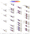 |
Fig. 3 Sequence of 15 GHz VLBA images from the MOJAVE program where we represent total intensity contours (3σ above background) with overlaid maps of polarized intensity (5σ above background) and corresponding EVPA information drawn as vectors on top. The length of the vectors is proportional to the polarized intensity. Gaussian model-component positions are indicated as orange crosses. The average size of the circular model components is ~0.3 mas for all epochs with a minimum size of zero mas at the core. |
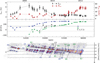 |
Fig. 4 Top panel: MOJAVE light curve with the total flux density (black triangles, for the most significant total flux density, 5σ above the background) and the total polarized flux density (dark red squares, integrating the flux densities of all model components with at least 1.4 mJy, which corresponds to the average baseline polarized flux density at 3σ above the background); middle panel: temporal evolution of the EVPAs of the polarized features A (blue), B (green), and C (black). The solid gray line at ~63° corresponds to the jet position angle derived from the average angle followed by all tracked components. The two thin gray lines at 63°–90° and 63°+90° mark anglesperpendicular to the jet axis. The EVPAs are flux-weighted averages for the corresponding feature; bottom panel: total intensity contours with overlaid color-coded maps of polarized intensity as shown in Fig. 3. Polarized model components forming the two main polarized features A and B and their near-ballistic trajectories are shown on top of the maps. Components that contribute to the extended most downstream polarized region of feature B but where no consistent kinematic model can be found are not labeled. |
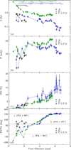 |
Fig. 5 Derived quantities of the total flux density (panel a), the polarized flux density (panel b), the degree of polarization (panel c) as well as the EVPAs (panel d) over core distance for the two major polarized features, A (blue) and B (green), together with the components C 1/C 2 (black). We use the mean flux-weighted core distance of all model components within each feature in a given epoch to describe the core distance of that feature. All quantities are averaged over the contained model components. The different EVPA evolutions are matched by occasional shifts of 180°. |
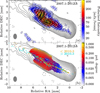 |
Fig. 6 Stacked images with polarimetry information for all involved epochs from early 2007.1 until mid 2012.5. We first stack the maps of the channels Q and U and then combine those to derive the shown maps. Panel a: color-coded distribution of the polarized intensity with overlaid EVPAs on top of total intensity contours in gray. White contours correspond to the polarized intensity. Panel b: distribution of the degree of polarization and overlaid Gaussian (total intensity) model components color-coded for components occurring before and after 2010.3 in orange and blue, respectively. |
3.1.2 Kinematic analysis
We can describe the dynamics of the polarized features A–C quantitatively by I) modeling the total intensity emission with a small number of Gaussian components (following Großberger 2014); II) measuring the linear polarization of these Gaussian components; and III) performing a kinematic study of components with significant polarization. For the latter, we constrain ourselves to components with a polarized flux density of at least 1.4 mJy, which, on average, corresponds to a 3σ detection with respect to the background. We reduce this lower threshold to 1 mJy, that is, 2σ only in case of model components that can be tracked over more than four epochs.
Most of these components follow near-ballistic trajectories with similar PAs (Fig. 4). Table 1 lists the polarized components with inferred proper motions on the sky. The distances of the selected polarized components and the unpolarized jet model components as a function of time are shown in Fig. 7. The leading components of the features A and B (A 1/A 2 and B 1/B 2, respectively) can be tracked over almost the full time range, and constantly dominate both the total and polarized flux densities of the parsec-scale jet (Fig. 8)6. The total flux density evolutions of the components A 1 and B 1 are considerably different. A 1 can be tracked over all 36 epochs and only slowly decreases in flux. The component B 1, in contrast, fades within seven epochs. The polarized flux density of both A 1 and A 2, as well as B 2, rapidly increase during their first epochs, which gives rise to the observed peaks in the integrated polarization light curve Fig. 5 (panel b) at around 2–3 mas. The components A 3 to A 7 and B 3 to B 11 form behind the leading components of both polarized features and their flux densities are overall lower. We therefore identify them as trailing components (Agudo et al. 2001) in the wake of the leading components similar to those observed by K08 after the 1996 outburst of 3C 111.
The leading components A 1 and B 1 are both found on ballistic trajectories in (x∕y)-space with position angles (PAs) of about 66° and 63°, and show comparable proper motions of 1.731 ± 0.016 mas∕yr and 1.67 ± 0.06 mas∕yr, respectively (see also Figs. C.1 and C.2). This is again similar to the speed of the leading component associated with the 1996 outburst (see K08). The components A 2 and B 2 follow PAs of about 68° and 64°, respectively. The PA of A 2 changes to about 58° after 3–4 mas. While we find a proper motion of 1.48 ± 0.01 mas/yr for B 2, A 2 cannot be described ballistically but shows signs of moderate acceleration in the longitudinal direction from 1.30 ± 0.14 mas/yr (<3 mas) to 1.56 ± 0.09 mas/yr (3−4.5 mas) before decelerating again to 1.28 ± 0.02 mas/yr (<3 mas). A similar behavior may be inherent to the component A 1, despite being statistically insignificant. We therefore remain with a ballistical description of A 1.
In both polarized features (A and B), we find components with slower proper motions being formed early on (A 3: 0.91 ± 0.16 mas/yr; B 3: 0.80 ± 0.12 mas/yr), both rapidlydecreasing in flux density (see Fig. 9). The component A 3 loses more than half of its flux density from ~200 mJy to ~80 mJy within less than half a year, while B 3 shows a more drastic decrease in flux density of a factor of five from ~900 mJy to ~250 mJy over four months. This is reminiscent of the similar behavior of component “F” in K08. The total flux density of both A 3 and B 3 starts off larger than that of the leading components A 1 and B 2, which increase in flux density during the decreasing evolution of A 3 and B 3.
In general, all components in the wake of A 1/A 2 and B 1/B 2 have lower proper motions than the leading components (between 0.8–1.4 mas/yr). Also, their inherent amount of variability both in total and polarized flux density is overall larger. Amongst these trailing components, the component A 4 forms immediately after 3 mas from the core with a proper motion of 1.40 ± 0.04 mas/yr and follows a trajectory with a PA of 68.3 ± 0.5°. It subsequently appears to split into A 5 and A 6 at around 4.5 mas from the core, which continue along different PAs of 59.3 ± 0.4° (A 5) and 62.8 ± 0.3° (A 6) at smaller velocities of about 1.0 mas/yr. If the components A 4–A 6 described the same underlying perturbation, we could put them into context with component A 2, which shows decelerating behavior downstream of approximately 4.5 mas. Their changing PAs, however, challenge this interpretation.
The polarized feature B describes the most stable polarized region that becomes increasingly complex in later epochs, eventually dominating the polarized intensity of the entire jet. The components B 2 and B 4seem to emerge out of a single unresolved component with an initial flux density of 1.15 Jy in epoch 2008.6, with B 2 becoming the more dominant and faster component in subsequent epochs (B2: ~1.5 mas/yr; B 4: ~1.1 mas/yr). Figure 10 shows the trajectories of both these components. The figure also includes two components that are observed and identified over the course of the 2007 outburst with help of higher-resolution observations with the Global Millimeter VLBI array by Schulz et al. (in prep.). The components B 2 and B 4 at 15 GHz appear as a continuation of these components at 86 GHz. Their velocity difference might reflect a shear within the plasma that we observe as feature B (cf. Discussion).
List of all polarized model components as part of the polarized features A and B with corresponding proper motions in units of mas/yr.
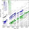 |
Fig. 7 Distances over time for all Gaussian model components required to fit the total intensity visibility data of all analyzed MOJAVE epochs (gray). In color, we only show model components describing the polarized features A (blue) and B (green), if their polarized flux density exceeds the given threshold of 1.4 mJy (3σ). In casesof components that are tracked over more than four epochs, we set a threshold of 1.0 mJy (2σ). The two leading components A 2 and B 2 are highlighted with large, filled squares. The two components A 3 and B 3 that form in the wake of these leading components during the first epochs of the features A and B, but fade quickly, are denoted as stars. We do not trace in detail the evolution of components in the wake of B 2 after 2011.4 due to the increased complexity of the polarized brightness distribution that cannot entirely be described by ballistic Gaussian model components. |
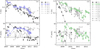 |
Fig. 8 Evolution of the total (panels a) and polarized flux density (panels b) for selected components of group A and B. For all components the total flux decreases with time. Components identified as trailing components are held in gray. The 2σ (3σ) thresholds for polarized components to be considered in Figs. 5 and 7 are denoted as solid (dashed) black lines. |
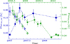 |
Fig. 9 Flux density evolution of the short-lived components A 3 (blue stars) and B 3 (green stars) together with the leading components A 1 (blue circles) and B 2 (green circles). Due to their different appearance times, the time axes of both components are different. |
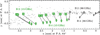 |
Fig. 10 (x, y)-plot emphasizing the components B 2 (triangles) and B 4 (diamonds) projected on a PA of 64° as observed at 15 GHz. The positions of all other model components at 15 GHz are drawn in gray. Solid gray lines connect the positions of B 2 and B 4 at the same epochs. Gray symbols resemble model components found at 86 GHz further upstream (Schulz, priv. comm.) that we relate with the components B 2 and B 4 at 15 GHz. |
3.2 Analysis of the brightness temperature distribution
We have shown above that the evolution of the EVPAs of both features A and B behave similarly with time and core distance. The consistent orientation parallel to the jet around 3–4 mas from the core and the foregoing drastic increase in polarized flux density lead us to further study this region. Figure 11 shows the dependence of the brightness temperature TB and the sizes of the circular Gaussian model components d on the core distance r.
The brightness temperature has been shown to follow a power law over core distance for samples of AGN jets (Kadler 2005; Pushkarev & Kovalev 2012), for the particular case of 3C 111 (K08) and for other individual sources (e.g., NGC 1052: Kadler et al. 2004; or S4 1030+61: Kravchenko et al. 2016). We note, however, that the RadioAstron Space VLBI resolution allows us to come even closer to the apparent jet base and delivers higher brightness temperatures as expected (e.g., Gómez et al. 2016; Kovalev et al. 2016). If the magnetic field B ∝ rb, the particle density N ∝ rn and the jet diameter d ∝ rl evolve like power laws with distance r from the core, the brightness temperature can be describedas TB ∝ rs (Blandford & Königl 1979, K08). The power-law index s (with s < 0) can then be expanded as
 (1)
(1)
where α is the spectral index, characterizing the flux-density spectrum via Sν ~ ν−α.
Figure 11 makes clear that this simplified ansatz can successfully describe the measured brightness temperature and jet diameter. We adopt uncertainties of 0.05 mas for r, 15% on TB and 0.01 mas on d, which corresponds to the scatter of all measured major axes. A sudden decrease of the model component sizes is apparent at a distance of around 3 mas from the core. This jump is accompanied by a jump in TB at that distance for the two components A 2 and B 2 that probe this transition region. We find the size of the component A 2 to decrease from 0.43 ± 0.03 mas to 0.352 ± 0.004 mas and for component B 2 from 0.43 ± 0.02 mas to 0.275 ± 0.003 mas when extrapolating the measured power-laws to the discontinuity at around 3 mas. The extrapolated brightness temperatures increase from  K to 1.03 ± 0.09 × 10¹⁰ K for A 2 and from
  K to
K to  K for B 2. For constant flux, two measurements of the brightness temperature, that is, TB,1 and TB,2, are related to the corresponding component sizes d1 and d2 by
  . We find TB,1∕TB,2 = 0.8 ± 0.3 and
  for component A 2 as well as TB,1∕TB,2 = 0.57 ± 0.16 and
  for B 2. Within the uncertainties, the sudden decrease of the component sizes is consistent with the increase of TB for adiabatic knots. The other plotted components have an insufficient number of traceable counterparts upstream or downstream of 3 mas and do not add further information to these results.
In Table 2 we list the measured indices l and (s − l) upstream and downstream of 3 mas. We exclude component B 8 from the fits. It describes an unrealistically steep power law, probably a result of its strongly variable flux density. Compared to a free expansion (l = 1), we find reduced expansion rates upstream of 3 mas. Beyond 3 mas, however, we find several components with indices as high as 1–3, averaging ~1.7. The index combination (s − l) is a measure of the gradients of the magnetic field and the gas density; it shows moderate values upstream of 3 mas and extremely steep values beyond.
To characterize the influence of α on s, we calculatespectral-index maps between 15 GHz and 43 GHz (BG data). We chose four separate epochs during which jet plasma components occupy the region beyond 3 mas and for which closely separated7 observations at 15 GHz and 43 GHz are available. We compare flux-weighted positions of optically thin regions of the total intensity maps to determine a core shift of RA = −0.22 and Dec = −0.09 between thetwo maps (cf., e.g., Kadler et al. 2004). Both maps are restored with a common beam enclosing the two single beams at 15 GHz and 43 GHz. The exemplary map in Fig. 12 reveals a pronounced gradient from an optically thick core with a flat power-law spectrum towards optically thin jet emission with α ~−1 downstream of 3 mas – a behavior that is observed in all four analyzed spectral index maps at different times. As a cross-check, we extract the integrated flux densities from the emission region downstream of 3 mas for both the restored 15 GHz and 43 GHz maps and calculate the averaged spectral index using the flux-density ratios. We derive consistent values of α ~−1 for all four tested epochs.
The parameter b describes the geometry of the magnetic field and cannot be directly measured with our data. In the idealized cases of a pure toroidal field, a value of b = −1 would apply. Similarly, b = −2 would describe a pure axial field. For these two cases, we can use the measurements of s − l and α to constrain the gradient of the particle density along the jet. We consistently find power laws rn with the index steepening at the distance of 3 mas from the core from n<3 mas ~−0.2 (1.8) to n>3 mas ~−2.1 (−0.1) for component A 2 and from n<3 mas ~−0.6 (1.4) to n>3 mas ~−3.6 (−1.6) for component B 2. The numbers consider a magnetic field with b = −1 (b = −2).
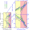 |
Fig. 11 Brightness temperature and major axis size against the core distance for all model components of all epochs (gray). The colored symbols correspond to model components that can be associated with the polarized features A and B. The components A 2 and B 2 probe the transition region at around 3 mas and are therefore emphasized with enlarged squares of white filling. Lines correspond to linear regression fits of data up- and downstream of 3 mas. |
Slopes for a power-law relation between the size of the major axis, d, and the brightness temperature TB against the core distance r (∝ rl and ∝ rs) in log–log space.
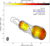 |
Fig. 12 Spectral index maps for quasi-simultaneous observations at 43 GHz (BG, epoch 2008-09-10) and 15 GHz (MOJAVE, 2008-09-12). Both maps are restored with a common beam shown on the bottom left and the spectral index α = log S1∕S2∕log ν2∕ν1 is computed accordingly for each pixel. The required shift of the 43 GHz map relative to the one at 15 GHz is − 0.22 mas in right ascension and − 0.09 mas in declination. The shift is determined by matching the flux-averaged mean x/y positions of the brightest components in both individual maps, excluding the core. |
4 Discussion
We have reported on the evolution of two features, A and B, both strong in total and polarized intensity through the VLBI jet in 3C 111. Their evolution follows a similar pattern for both groups of components between 2 and 6 mas, which is largely consistent with results from K08 and an independent study by Homan et al. (2015), who suggest a very similar velocity pattern with signs for accelerated motion upstream of 3–4 mas and decelerated motion beyond. In the following we discuss our results and describe possible scenarios that could explain these observed jet features, which most likely reflect shocked plasma. Therefore, the observed and derived jet-intrinsic quantities cannot be interpreted as those describing an unperturbed flow.
4.1 Inner 2 mas from the core
Schulz et al.(in prep.) report on very-high-angular-resolution GMVA observations of the inner 2 mas of the jet of 3C 111 during the outburst that has led to the ejection of the components associated with feature B. In Fig. 10, we show the positions of the 86 GHz model components that can be associated with the 15 GHz jet components B2 and B4 on the basis of their temporal evolution at both frequencies. The 86 GHz images show a highly complex structure and dynamical evolution of the individual jet components on these small scales.
4.1.1 Possible effects of Faraday rotation
The unresolved knots that emerge from the compact core region at 15 GHz become polarized while they propagate along the jet. Beyond 2–3 mas, the degree of polarization quickly rises to a level of about 5% as shown in Figs. 5 and 6. Such a steep transition is unlikely to arise from a smooth gradient in optical depth along the jet (see, e.g., Porth et al. 2011). Instead, the originally low degree of polarization can be understood as a result of depolarization upstream of 2–3 mas in a foreground Faraday screen (see, e.g., Gómez et al. 2008, for the case of 3C 120). In addition, beam depolarization due to multiple polarized components close to the unresolved core might play an important role given the complex and bent jet structure seen at 86 GHz (Schulz et al. 2012). Both possibilities are supported by the strongly variable EVPAs in the inner 2 mas with a dynamic range of as large as 90° over 2 mas (see Fig. 5, panel d).
Here, we test for the effects of Faraday rotation as a cause of those changes8. Figure 13 shows the polarized flux-density distribution for the same two quasi-simultaneous epochs at 15 GHz (MOJAVE) and 43 GHz (BG data) for which the spectral index distribution was calculated in Fig. 12. In both maps, we are sensitive to polarized intensity upstream of 2 mas.
Panels cand d of Fig. 13 show a strongly changing and double-peaked RM gradient along the jet ridge line (see the green open squares in panel d). The RM changes rapidly between the core and 2 mas distance with a maximum of ≈ − 8000 rad/m2 just before 1 mas. Following a dip down to 50–100 rad/m2, a second peak appears around 1 mas at ≈ − 5000 rad/m2. The RMs of the two peaks correspond to EVPA rotations of roughly 180° and 40°, respectively, where the first can be compensated with the ambiguity of π. The high values obtained for the RM within this region are consistent with recent results by Kravchenko et al. (2017) for a large sample of jets.
The strong variations in the EVPAs observed upstream of 2 mas (Fig. 5) also agree with the observed RM inhomogeneities in that region. The observed inhomogeneous RM map (see Fig. 13) could be related with an external Faraday screen (e.g., Gómez et al. 2000, 2008), for example, NLR clouds in the line of sight (O’Dea 1989; Wardle 1998).
Nevertheless, the tentative transverse RM gradient (e.g., Asada et al. 2002, 2010; Croke et al. 2010; Hovatta et al. 2012; Gabuzda et al. 2014) can also be an independent tracer for an underlying helical field. The detection of consistently negative circular polarization for the core of 3C 111 in MOJAVE data (Homan et al. 2006) gives an independent argument for the presence of an ordered magnetic field configuration at the core region.
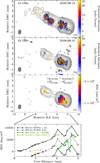 |
Fig. 13 RMmap (panel c) between two adjacent maps at 15 GHz/MOJAVE (panel a) and 43 GHz/BG (panel b) that have also been used to calculate the spectral index in Fig. 12. The polarized emission is overlaid in color on top of the total intensity contours, both at a baseline intensity of 3σ. We only calculate values of RM where we detect polarized emission >3σ both at 15 GHz and 43 GHz. We apply the same relative core shift between the maps at both frequencies as estimated for Fig. 12 and the identical envelope beam. Panel d shows RM cuts along the indicated ridge lines for our measurement upstream of 2 mas (green squares) and for a measurement by Zavala & Taylor (2002) between 3.5 mas and 4.5 mas (orange triangles). We also show as black solid and dashed lines the RM distribution along the jet that is required to explain the observed EVPA evolution of feature B (Fig. 5) with respect to either an intrinsically perpendicular or parallel field, respectively. The two RM distributions shown for an intrinsically perpendicular field reflect the ambiguity of π. |
4.1.2 Intrinsic magnetic-field orientation
Basic jet models typically predict EVPAs, which are either parallel or perpendicular to the overall jet flow. Intrinsically parallel EVPAs are allowed in cases with an axisymmetric helical magnetic field depending on the viewing angle and the pitch of the helix (Lyutikov et al. 2005; Lyutikov & Kravchenko 2017). Lyutikov et al. (2005) computed the expected EVPA configuration for jets being threaded by a helical field of decreasing pitch angle towards its fast spine. The larger spine emissivity causes observed EVPAs to be always perpendicular to the jet. Similar conclusions are drawn from RMHD simulations for the selected jet velocities, intrinsic pitch angles, and viewing angles, where a helical field is filled with plasma (e.g., Roca-Sogorb et al. 2009; Gómez et al. 2016).
Here, we investigate the implications of the measured RM for the intrinsic EVPAs in the inner jet region. We assume for simplicity that the RM shield is stable over time, and we can tentatively infer the intrinsic EVPAs (but see caveats discussed below). Figure 13 shows the RM that is needed to have the intrinsic EVPAs of feature B be aligned parallel to the jet and perpendicular to the jet, respectively. In the former scenario, we find a fairly good overall agreement with the measured RM values (the region of the dip in RM is not probed), while the scenario with perpendicular EVPAs predicts systematically overly high RM values upstream of ~5 mas from the core. Our measurements thus show that underlying parallel EVPAs can explain the observed RM gradient and the EVPA rotation over distance in the inner-jet region upstream of about 1.5 mas. The lack of a complete coverage with RM data, however, does not allow us to conclude on the bulk of the EVPA rotation at >2 mas.
At this point, we have to note several caveats with respect to the calculated RM values in Fig. 13. First, the use of only two frequencies introduces strong uncertainties on the measured RM values and the simple λ2 -law may be broken close to the core depending on the structure and geometry of the screen (Kravchenko et al. 2017). Furthermore, by measuring the RM coincident for the well polarized feature B, we are sensitive only to the shocked plasma of a single epoch and not the quiescent flow. We are therefore lacking sufficient RM information for the entire parsec-scale jet both in space and time. For these reasons, we abstain from attempting to directly correct the measured EVPAs in Fig. 5.
4.1.3 Component evolution and kinematics
The leading components of both features are divided into three sub-components in our modeling and show different behaviors: although B1 fades in brightness very quickly, A1 persists and maintains its brightness across most of the observing epochs. In both cases, the components A2 and B2 dominate in brightness further upstream. B2 becomes the leading component of the feature B after B1 disappears. In addition, the components A3 and B3 appear as bright features that fade rapidly and disappear after four epochs, which follows a similar behavior to that reported for component “F” in K08. The components E and F were studied in terms of the hydrodynamical structure of the perturbation by Perucho et al. (2008). These authors could successfully explain the evolution of those two components, which were the only ones used to model the region. Thus, although our current modeling shows a more complex system of components, it seems to indicate that components A1 and B2 would correspond to E, whereas components A3 and B3 would correspond to F in the interpretation given by Perucho et al. (2008). However, the richness of the structure revealed in this work suggests that more detailed numerical simulations should be performed, which is beyond the scope of this paper.
4.2 The region between 2 and 4 mas
Downstream of approximately 2 mas from the core, the jet is transversely resolved. Here, we observe a systematic smooth swing of the overall EVPAs of the polarized features A and B as they propagate with the jet flow. At the same time the jet overall structure is remarkably straight and individual components show only small deviations from their original trajectories (see Appendix A and the component positions shown in the bottom panel of Fig. 6): this, in principle, leaves the interpretation of the evolution in this region open to the possibility that some components follow bent trajectories. However, the amplitudes of these changes and their contribution to the polarized emission are small, and therefore we neglect their influence on the large observed EVPA rotation, which has been claimed to be an explanation for other sources (Agudo et al. 2007; Molina et al. 2014; Lyutikov & Kravchenko 2017). This also includes the intrinsic near-perpendicular viewing angle (see Appendix A), which makes a projected geometrical EVPA rotation unlikely in the present case. We cannot, however, exclude effects due to an inhomogeneous distribution of emitting plasma across the flow; Fig. 6 indicates that different areas of the jet cross-section are lighting up at different times. These areas also include component trajectories that do not follow the main stream. A discussion of related higher-order effects, however, lies beyond the scope of this paper. In the following subsection, we show that the results stated in this paper can be explained by a recollimation shock within this region plus shearing of the jet flow.
4.2.1 A possible recollimation shock
In Sect. 3.2 we showed evidence for unusual behavior at around 3–4 mas from the core, that is, a sudden decrease of the feature size d at a distance of about 3 mas, accompanied by an increase of the brightness temperature TB (similar to Roca-Sogorb et al. 2009) and the polarized flux density of individual model components. We recall that the power-law exponent describing the evolution of the jet radius over distance changes from values smaller than 1 to larger than 1 around 3 mas. These observations can be interpreted in terms of the presence of a recollimation shock at about this distance, which was already suggested by K08. Such recollimation shocks are naturally forming extended structures in overpressured jets as shown by numerical simulations (e.g., Gómez et al. 1997; Mizuno et al. 2015; Fromm et al. 2016; Martí et al. 2016).
In the analysis that we have presented in Sect. 3.2, we provide estimates of the parameters s, l, and α involved in the relation s − l = n + b (1 − α). Since we cannot constrain the index b, we provide estimates for the resulting particle density evolution in Sect. 3.2 for both a toroidal (b = −1) and an axial (b = −2) field in a conically expanding jet (Pushkarev et al. 2017). Independent of the choice for b, our results show a steepening of the particle density described by a power-law with the index n, possibly indicating the expected expansion after a recollimation.
4.2.2 The rotation of the EVPAs
The stacked polarization maps in Fig. 6 reveal a large swing of about 180° already starting in the inner jet region, related with the passage of the components. When assuming the presence of a conical recollimation shock, the rotation could thus be explained in terms of the bright features evolving into and out of the tip of the conical shock. Unfortunately, RMHD simulations that tackle this scenario are still missing.
Using calculations described in Cawthorne (2006), Agudo et al. (2012) could successfully explain the particular EVPA distribution of a standing feature (associated to a recollimation shock) in 3C 120 with a radial or Y-shaped pattern of EVPAs being aligned along the central ridge and oblique EVPAs towards the edges. Cawthorne et al. (2013) observe a similar pattern for the core of S5 1803+784, equally arguing for the presence of a recollimation shock from their modeling. In steady situations, that is, when there is no interaction with a traveling component, these results demonstrate the peculiar influence of conical shocks on the observed polarization signatures. For 3C 111 the situation is clearly more complex, probably involving a shock-shock interaction (see, e.g., Fromm et al. 2016, for a relativistic hydrodynamics study).
Contrary to the predictions by steady-state jets that form weak recollimation shocks (Roca-Sogorb et al. 2009; Gómez et al. 2016), our RM data favor intrinsically parallel EVPAs in the inner jet region (≲1.5 mas). Farther downstream in the jet, Zavala & Taylor (2002) also observed a gradient in RM, but at lower values smoothly ranging from − 800 rad/m2 to − 200 rad/m2 between 3 and 5 mas (see Fig. 13)9, which is consistent with typical values of RM obtained for the MOJAVE sample (Hovatta et al. 2012). Comparing with our measurement at 2 mas from the core, the RM appears to be rather flat and stable along the outer jet. When extrapolating RM found by Zavala & Taylor (2002) to 1.5 mas and 6 mas, Fig. 13 suggests intrinsically perpendicular EVPAs in these regions.
The flatness and structural stability of the RM in the 2–4 mas region is in contradiction with it causing the large EVPA rotation. We can tentatively address a simple explanation for this continuous rotation of the EVPAs.
-
Between ~1.5 and 2 mas, the RM departs from the one corresponding to an underlying parallel orientation of the EVPAs and approaches an intrinsically perpendicular orientation (see Fig. 13), because the measured RM translates into small rotations of the EVPAs. This initial rotation can be related to the shearing observed between components B2 and B4 between 1 mas and 3 mas (Fig. 10). The components are located at a central and peripheral position in the jet, respectively, and show different velocities, with the central component, B2, being faster. Observations at 86 GHz of the same flaring event leading to the B feature (Schulz et al., in prep.) show that these components are most probably individual ejections within the flare. These components are caught up by our observations, showing differential dynamics that possibly reveal a transverse structure of the jet velocity. The shearing of the jet plasma can explain the generation of a strong poloidal field component, resulting in a dominating perpendicular orientation of the EVPAs. This effect has previously been proposed by, for example, Laing (1980, 1981), Cawthorne et al. (1993a), and Wardle (1998). The frequent observation of perpendicular EVPAs at the jet boundary and aligned EVPAs at the center seems to confirm a scenario where the sheared-layer stretching of the field lines dominates (O’Dea & Owen 1986; Attridge et al. 1999; Giroletti et al. 2004; Pushkarev et al. 2005). Differential flows have also been observed in simulations of parsec-scale jets that show the stretching of lines at the jet shear layer (Roca-Sogorb et al. 2009), and in MHD simulations of kiloparsec-scale jets, which show this effect for the whole jet cross-section (Matthews & Scheuer 1990; Gaibler et al. 2009; Huarte-Espinosa et al. 2011; Hardcastle & Krause 2014).
-
If strong planar shocks are traveling along the spine, we expect them to appear as bright components, such as B2, and show increased polarized emission with parallel EVPAs. At the interaction with the conical standing shock, this region becomes even brighter and can therefore explain the observed alignment of the EVPAs around 3–4 mas.
-
Finally, downstream of the recollimation shock, the flow progressively returns to the pre-shock situation, in which the polarized emissivity is dominated by the sheared region, with dominant perpendicular EVPAs.
We note that in the picture of an unsheared axisymmetric helical field (e.g., Lyutikov et al. 2005), the observed intermediate EVPAs cannot be described solely by changes in the pitch angle of the helix (see Appendix B) but potentially by the interaction of the propagating shock with the recollimation shock – a question that future RMHD simulations need to answer. The dynamic nature and complexity of the process must therefore be disassociated from the toy model shown in Fig. B.1, which can successfully explain a dichotomy between a parallel and perpendicular orientation but not the continuous distribution of EVPAs.
4.2.3 Estimate of the Mach number and magnetization
If the change in the EVPA direction is caused by the presence of a recollimation shock, we can obtain valuable insight into the jet parameters by knowing the location of different standing shocks as well as their transverse extent (Martí et al. 2016). There are indications for standing features within the inner 0.5 mas of the jet (see Fig. Fig. 7). Both Schulz et al. (in prep.) and Jorstad et al. (2017) find similar standing features at 86 GHz and 43 GHz, respectively. The evidence collected indicates the presence of a first recollimation shock in close vicinity to the millimeter core and a second one at around 3 mas, that is, the detection of multiple recollimation shocks in 3C 111, similar to, for example, BL Lac (Gómez et al. 2016; Mizuno et al. 2015), CTA 102 (Fromm et al. 2013, 2016) or 3C 120 (León-Tavares et al. 2010; Roca-Sogorb et al. 2010; Agudo et al. 2012). Based on this evidence, we can estimate the magnetosonic Mach number and put qualitative constraints on the magnetization of the flow (see also Nokhrina et al. 2015, for independent estimates of the jet magnetization).
We can use the inferred distance of ~3 mas between the 15 GHz core and the downstream recollimation as an approximation to the distance between two shocks (see Fig. 14)10. The deprojected separation corresponds to 7.6–18.6 pc, depending on the jet viewing angle (see Appendix A). This translates to 2.2–5.3 × 10⁵ rs. Although this recollimation shock is likely not the first one along the jet, the order of magnitude compares well with distances of recollimation shocks of around 105 rs for the examples of M87, CTA 102 or BL Lac.
Martí et al. (2016) performed RMHD simulations to study the internal structure of overpressured jets that form a series of recollimation shocks, covering a wide range of the jet magnetization and internal energy. They report on the correlation between the magnetosonic mach number  and the half-opening angle of the flow
  (with R the jet radius at its maximum expansion and D the distance between two recollimation shocks). We find that the jet of 3C 111 is resolved at 3 mas (see Fig. 11) with a maximum FWHM of approximately ~1 mas. This value gives a lower limit to the jet expansion radius because 1) the jet flow can be wider than the visible radio jet, and 2) the location of the maximum jet expansion is unknown. Therefore, from this value and the distance between shocks, we obtain an upper limit of
  . The values that we obtain are
 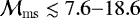 .
.
The magnetosonic Mach number itself is defined as
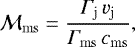 (2)
(2)
with Γj being the Lorentz factor of the jet, Γms the Lorentz factor associated with the magnetosonic speed cms, and vj, the jet speed. The observed superluminal components and the large internal jet speed estimated in Appendix A allow us to approximate vj ≃ c. Thus, using c = 1,  . The values obtained for the magnetosonic Mach number (≲7.6–18.6) allow us to approximate Γms ≃ 1 as otherwise the bulk Lorentz factor needs to be large (≤20). Finally, we obtain
  . Under these assumptions and considering Fig. 15 from Martí et al. (2016), the jet will be kinetically dominated for bulk Lorentz factors Γj ≳ 4.8−11.6 (depending on the deprojected distance between the shocks; see above). These values are of the order ofthose observed (see Appendix A). When we insert the lower limit on the jet speed vmin ~ 0.976 c close to the inclination angle of θmin = 10° and the corresponding upper limit on the Mach number
  into Eq. (2), we can establish a lower limit of cms,min = 0.23. Independentmeasurements of the jet speed and inclination angle by Jorstad et al. (2005) and Hovatta et al. (2009) result in magnetosonic speeds of cms = 0.38 and cms = 0.53, respectively,favoring a jet being kinetically dominated or just at the transition of being Poynting-flux dominated (Martí et al. 2016).
 |
Fig. 14 Illustration of the relevant observed features mixed with the theoretical prediction of a continuously expanding and recollimating flow (e.g., Daly & Marscher 1988; Gómez et al. 1997) with an entrained particle distribution of downstream decreasing density. The straight lines indicate Mach cones for different speeds of the flow. Standing features observed at 43 GHz and 86 GHz are interpreted as the first recollimation shock downstream of and in close vicinity to the cores atthese frequencies. Its distance to the black hole is unknown for 3C 111. At 15 GHz, we observe a second recollimation shock at a distance of 3 mas from the core component at that frequency. We detect no signs for further recollimations. Overlaid, we plot the EVPAs from the stacked image in Fig. 6. The orientation of these EVPAs appears to be perpendicular to the jet in absence of the recollimation and parallel on top of it. |
4.3 The jet beyond 4 mas
The region downstream of the recollimation is characterized by a smooth and consistent 90° eastward swing of the EVPAs of both features A and B from being aligned with the jet at the recollimation to a perpendicular orientation. This swing has been explained in the previous section with a helical field stretched out towards being poloidally dominated due to a velocity shear caused by the bulk flow of the jet. Such a field would give rise to EVPAs being predominantly oriented perpendicular to the jet, which is also predicted by numerical simulations (e.g., Huarte-Espinosa et al. 2011; Hardcastle & Krause 2014). Sample studies, moreover, have revealed transverse EVPAs to be typical features for FR II jets (Bridle 1984; Hardcastle et al. 1997; Gilbert et al. 2004). Also, results by Lister & Smith (2000) and Kharb et al. (2008) suggest thatoverall transverse EVPAs are found in presumable quiescent quasar jets, as opposed to shocked quasars, where a larger fraction of parallel EVPAs have been found. Furthermore, Perucho et al. (2005); Martí et al. (2016) have shown that the presenceof a shear layer slows down the growth of Kelvin-Helmholtz or current-driven instabilities, providing the jet with increased stability, as expected for FRII jets like 3C 111. Observational evidence is provided, for example, by Kharb et al. (2008); Gabuzda et al. (2014), and, in the case of 3C 111, by K08. This effect reinforces the dominance of transverse EVPAs (before and) after the interaction of the traveling features with the standing shock.
Beyond the suggested recollimation shock, the expansion rate increases to values larger than one (see Sect. 3.2). Also, the density gradient becomes steeper, as obtained from the evolution of the component diameter and brightness temperature with distance. These results seem to indicate a freely expanding jet, possibly because of a steepening of the ambient pressure profile, compatible with the interpretation of foregoing MOJAVE data by K08. We also find a number of new components that form in the wake of the leading components A 2 and B 2. These new components can be interpreted as trailing features (Agudo et al. 2001; Jorstad et al. 2005). The oscillation that is produced in the rear of the leading component can affect the entire jet cross-section and can be strong enough to produce conical shocks, which themselves propagate downstream and are sufficiently bright to be detected (Agudo et al. 2001; Mimica et al. 2009).
5 Summary and conclusions
We have investigated the complex evolution of the 3C 111 jet flow that originated from millimeter-wavelength outbursts just before 2006 (outburst A), 2008 (outburst B), and 2009 (outburst C). As part of the flow, individual apparent superluminal features were tracked and characteristic parameters were recorded both in time and core distance, namely, the (polarized) flux density, brightness temperature and feature size. This dedicated study was facilitated by the increased density of the MOJAVE monitoring of 3C 111 and the availability of polarization information for all epochs. We summarize our key observational results as follows:
-
Upstream of ~2 mas the EVPAs are strongly variable with time. This variability has a potential de-polarizing effect, which can naturally be explained by the observed strong and inhomogeneous RM distribution across that region. Also, beam depolarization plays a role in that regard. When accounting for possible rotation, we infer intrinsically parallel EVPAs upstream of ~1.5 mas.
Within ~1.5–2 mas the Faraday-corrected EVPAs become transverse to the jet. We interpret this as produced by a shear at the boundary layers of the jet flow, that is, a differential transverse velocity structure leading to a dominant axial magnetic field in this region. Such a shear is supported by the peculiar kinematics of the jet components B 2 and B 4, which appear as the continuation of two components observed at 86 GHz for this same flaring event (Schulz et al., in prep.).
At 2–4 mas we find indications for a recollimation shock based on a sudden increase of the brightness temperature accompanied with a decrease in feature size for individual components. Also, the polarized intensity reaches large values in this region. Beyond this region, the power-law index describing the growth of the components increases moderately, while the particle density gradient steepens significantly. Our estimates of the magnetosonic Mach number based on the distance between standing components (Martí et al. 2016) put the parsec-scale jet well into the kinetically dominated regime, or just at the transition to being Poynting-flux dominated. Based on archival information, we conclude on a low and relatively flat RM gradient downstream of ~2 mas. We can therefore not explain the bulk of the EVPA rotation with a changing Faraday screen. Instead, our observation of aligned EVPAs at the recollimation as well as intermediate angles in between could likely be the result of the interaction of shocked ejecta with a standing shock that may be able to further enhance the toroidal field component.
Beyond 4 mas the stacked polarized maps indicate an extended region with significant levels of polarization (associated to the passing components) with an overall trend of EVPAs turning back into a transverse orientation. Similar to the situationaround 2 mas, we propose a boundary layer interaction causing a dominant axial field component following the possible reacceleration of the jet flow at the spine with respect to that at the boundaries. 3C 111 therefore fits well into the common frame of (quiescent and unperturbed) FR II jets, where jets typically show a dominance of transverse EVPAs. Furthermore, we also detect trailing features in this region that may represent secondary pinch mode perturbations in the wake of the leading shock.
3C 111 turns out to be a source that is uniquely well suited to probing the physics of the innermost parsec-scale jet by carefully mapping the distribution and long-term evolution of (polarized) intensity over a distance of tens of parsecs downstream. We find that the peculiar behavior and large rotation of the EVPAs (~180° across a distance of 4 mas, i.e., ≲25 pc deprojected distance) may be related to a deviation from the quiescent situation of a sheared jet flow, that is, the passage of shocks through a recollimation shock. Such an interaction, however, lacks corresponding RMHD simulations with full radiative output including polarization. We therefore propose the presented results as observational reference for future simulations.
Acknowledgements
T.B. is grateful for fruitful discussions with M. Lyutikov and E. Kravchenko, and thanks D. Gabuzda for her input that helped to improve the paper. We thank the National Radio Astronomy Observatory, a facility of the National Science Foundation operated under cooperative agreement by Associated Universities, Inc.; this research has made use of data from the MOJAVE database that is maintained by the MOJAVE team (Lister et al. 2009) and IRAM, which is supported by INSU/CNRS (France), MPG (Germany) and IGN (Spain). This work has benefited from research funding from the European Community’s Seventh Framework Programme. The Submillimeter Array is a joint project between the Smithsonian Astrophysical Observatory and the Academia Sinica Institute of Astronomy and Astrophysics and is funded by the Smithsonian Institution and the Academia Sinica. We also thank J. E. Davis for the development of the slxfig module that has been used to prepare the figures in this work. We made use of ISIS functions provided by ECAP/Remeis observatory and MIT (http://www.sternwarte.uni-erlangen.de/isis/) as well as the NASA/IPAC Extragalactic Database (NED), which is operated by the Jet Propulsion Laboratory, California Institute of Technology, under contract with the National Aeronautics and Space Administration. M.P. acknowledges financial support from the Spanish Ministerio de Economìa, Industria y Competitividad (grants AYA2013-40979-P, and AYA2013-48226- C3-2-P) and from the local Valencian Government (Generalitat Valenciana, grant Prometeo-II/2014/069). I.A. acknowledges support by a Ramón y Cajal grant of the Ministerio de Economía y Competitividad (MINECO) of Spain. A.B.P. and Y.Y.K. acknowledge partial support by the Russian Foundation for Basic Research (grant 17-02-00197), by the government of the Russian Federation (agreement 05.Y09.21.0018), and by the Alexander von Humboldt Foundation. E.R. acknowledges partial support by the Spanish MINECO project AYA2012-38491-C02-01 and by the Generalitat Valenciana project PROMETEOII/2014/057. T.S. was funded by the Academy of Finland projects 274477 and 284495. The research at the IAA-CSIC was supported in part by the MINECO through grants AYA2016-80889-P, AYA2013-40825-P, and AYA2010-14844, and by the regional government of Andalucía through grant P09-FQM-4784.
Appendix A: Constraints on the viewing angle and the intrinsic speed
We estimatethe viewing angle θ and the intrinsic jet speed β′ using the relation for the apparent speed
 (A.1)
(A.1)
We choose the observables measured for the components B 1−B 4 that describe the jet just downstream of the core in 2008. Their average apparent proper motion is 1.27 mas/yr, translating to βapp = 4.5 with 1 mas = 1.08 pc when applying the latest cosmological parameters from Planck Collaboration XIII (2016). We insert βapp in Eq. (A.1) and plot the solution for θ (β′) in Fig. A.1 as solid, black line. This line both defines the lower limit on the jet speed  , that is, β′ ≥ 0.976 and the upper limit on the viewing angle
 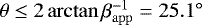 . Independent estimates of the viewing angle were derived by also measuring the Doppler factor via the decline time of ejected knots in addition to their apparent speed (Jorstad et al. 2005). They equally state a possible range of θ ~ 10−25° for a number of observed knots with a weighted average of 18.1°. This range is consistent with an upper limit of 20° found by Oh et al. (2015). We adopt the lower limit of 10° estimated by Lewis et al. (2005) for the large-scale morphology, although lower values cannot be excluded based on parsec-scale kinematics. Extending on the method used by Jorstad et al. (2005), Hovatta et al. (2009) estimate the Doppler factor based on Tb variability and find an inclination of about 15.5° when considering an apparent component speed of βapp ~ 5.9. Both proposed viewing angles are well consistent with our estimate.
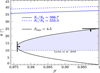 |
Fig. A.1 Constraints on the intrinsic jet velocity β′ and the inclination angle θ based on the average measured apparent speed βapp = 4.5 for the leading components B 1–B 4 of feature B. Two estimates for the jet-to-counterjet flux-density ratio S1 ∕S2 define further constraints drawn as blue lines. The blue-shaded region highlights the allowed parameter space, and the thick lines with corresponding arrows define the lower and upper limits on the jet speed and the inclination angle. |
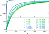 |
Fig. A.2 Constraints on the intrinsic viewing angle θ′ based onprevious estimates of the viewing angle in the observers frame and the intrinsic speed β′. We plot the relation θ′(θ) for a range of allowed values of β′. The lower limit of θ = 10° at a speed of β′~ 0.976 sets the lower limit on θ′. |
Figure A.1 also shows upper limits based on two estimates of the jet-to-counterjet ratio
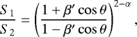 (A.2)
(A.2)
where α is the spectral index, which is calculated for the components B 1–B 4 between two MOJAVE epochs at 2008-09-12 and 2009-01-30 as well as quasi-simultaneous archival observations at 43 GHz. We find values of α = −0.75 and α = −0.92, respectively. The integrated flux density of these components at both epochs are S1 = 2.2 Jy and S1 = 1.4 Jy with corresponding estimates on the counter-jet flux density of S2 = 6.0 mJy and S2 = 4.2 mJy, respectively,when assuming an unresolved counter-jet, if it was detected. Both values of S2 are upper limits and correspond to 10σ of the background rms, which is a rather conservative choice. Our estimates using the flux ratios exclude viewing angles above ~35°, while better constraints on the counter-jet flux density could help to further constrain the maximum viewing angle of about 25° set by the measured apparent speed.
Using the estimate on θ, we can also constrain the intrinsic viewing angle to θ′ by using theLorentz-transformation
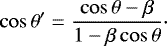 (A.3)
(A.3)
In Fig. A.2 we plot this function for a number of values of β′ ≳ 0.976. The lower limit on the viewing angle of 10° at a speed of β′~ 0.976 establishes the lower limit of θ′≳ 76.8°. When instead inserting the estimates by Jorstad et al. (2005) and Hovatta et al. (2009), who additionally constrain the Doppler factor from flux and TB-variability arguments, we find θ′~ 108° for Γ = 4.4, θ = 18.1° (Jorstad et al. 2005), and θ′~ 129° for Γ = 7.7 and θ = 15.5° (Hovatta et al. 2009).
Appendix B: Polarization signatures and a possible helical magnetic field
The lack of numerical simulations that tackle the interactions between moving and stationary shocks in a RMHD setup, forces us to discuss our results using simplifying assumptions. Lyutikov et al. (2005) consider an axisymmetric magnetic field constraining a hollow cylindrical jet and infer corresponding polarization properties.
Figure B.1 shows the expected, integrated degree of polarization for such an axisymmetric helical field in a hollow-jet geometry. We plot multiple solutions for a range of intrinsic pitch angles ψ′ between 20°–90° (from the bottom to the top). In the expression given by Lyutikov et al. (2005) negative and positive values correspond to orthogonal and aligned EVPAs, respectively.Above ψ′ = 50°, the field is getting toroidally dominated featuring EVPAs aligned with the jet. The degree of polarization will be maximal for a pure toroidal field with ψ′ = 90° a pure axial field for very low pitch angles. In summary, the EVPA distribution would appear as bimodal, depending on the dominant component, that is, the pitch angle of the field.
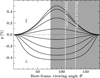 |
Fig. B.1 Degree of polarization for a range of rest-frame viewing angles θ′ onto axial-symmetric helical magnetic fields in a hollow cylindrical geometry. The estimated range of θ′ for 3C 111 is highlighted as gray-shaded region with two independent estimates as white, dashed lines based on inclination angles stated in the literature. Negative values of p correspond to an integrated EVPA perpendicular to the jet axis, positive values result in parallel EVPAs. The figure shows a range of intrinsic pitch angles ψ′ with steps of10° between 20°–90° from the bottom to the top. This example corresponds to the analytical expression provided for a particle distribution N(E) d E ~ Ep dE with p = 3 in Eq. (21) by Lyutikov et al. (2005). |
A 90° swing in theobserved EVPA can thus occur by changes in the intrinsic pitch angle. We warn the reader that this result is obtained using a determinate electron distribution exponent that allows for an analytical solution of the equations. Changes in the EVPA orientation can also occur with changing viewing angle only for a particle distribution of lower index (p < 3) and for a small range of pitch angles (Lyutikov & Kravchenko 2017). In addition, studies of large samples of blazars seem to confirm this quasi-bimodal distributions of EVPAs (Bridle 1984) with the majority of VLBI knots in BL Lac objects showing aligned EVPAs (Gabuzda et al. 1994, 2000; Lister & Smith 2000).
In Appendix A, we determine a lower limit on the intrinsic viewing angle of θ′ = 76.8° based on the range of viewing angles in theobservers frame of θ = 10−25.1°. The allowed range for θ′ with respectto our kinematics is shown as gray-shaded region in Fig. B.1. The independent estimates of θ′ ~ 108° and θ′ ~ 129° based on inclination angles proposed by Jorstad et al. (2005) and Hovatta et al. (2012) are marked as white dashed lines. Our observationsof a polarization degree of around 10–20% would be consistent with this model for pitch angles around 60–70° in case of a toroidal field or for pitch angles around 40–50° in case of an axial field.
Appendix C: Evolution of the model components in x∕y-space
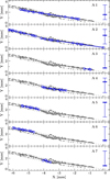 |
Fig. C.1 Model component positions in x/y-space for the feature A. In each panel, all model components are shown as gray circles in the background. The colored bar on the right of each panel denotes the average polarized flux of each component within the minimum/maximum fluxes of all components of the feature A, that is, 2.2/11.2 mJy. |
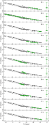 |
Fig. C.2 Model component positions in x/y-space for the feature B. In each panel, all model components are shown as gray circles in the background. The colored bar on the right of each panel denotes the average polarized flux of each component within the minimum/maximum fluxes of all components of the feature B, that is, 4.6/17.8 mJy. |
References
- Abdo, A. A., Ackermann, M., Ajello, M., et al. 2010, Nature, 463, 919 [NASA ADS] [CrossRef] [PubMed] [Google Scholar]
- Agudo, I., Gómez, J.-L., Martí, J.-M., et al. 2001, ApJ, 549, L183 [NASA ADS] [CrossRef] [Google Scholar]
- Agudo, I., Bach, U., Krichbaum, T. P., et al. 2007, A&A, 476, L17 [NASA ADS] [CrossRef] [EDP Sciences] [Google Scholar]
- Agudo, I., Gómez, J. L., Casadio, C., Cawthorne, T. V., & Roca-Sogorb, M. 2012, ApJ, 752, 92 [NASA ADS] [CrossRef] [Google Scholar]
- Agudo, I., Thum, C., Gómez, J. L., & Wiesemeyer, H. 2014, A&A, 566, A59 [NASA ADS] [CrossRef] [EDP Sciences] [Google Scholar]
- Agudo, I., Thum, C., Ramakrishnan, V., et al. 2018a, MNRAS, 473, 1850 [NASA ADS] [CrossRef] [Google Scholar]
- Agudo, I., Thum, C., Molina, S. N., et al. 2018b, MNRAS, 474, 1427 [NASA ADS] [CrossRef] [Google Scholar]
- Aller, H. D., Hodge, P. E., & Aller, M. F. 1981, ApJ, 248, L5 [NASA ADS] [CrossRef] [Google Scholar]
- Aller, M. F., Aller, H. D., & Hughes, P. A. 2003, ApJ, 586, 33 [NASA ADS] [CrossRef] [Google Scholar]
- Altschuler, D. R. 1980, AJ, 85, 1559 [NASA ADS] [CrossRef] [Google Scholar]
- Asada, K., Inoue, M., Uchida, Y., et al. 2002, PASJ, 54, L39 [NASA ADS] [Google Scholar]
- Asada, K., Nakamura, M., Inoue, M., Kameno, S., & Nagai, H. 2010, ApJ, 720, 41 [NASA ADS] [CrossRef] [Google Scholar]
- Attridge, J. M., Roberts, D. H., & Wardle, J. F. C. 1999, ApJ, 518, L87 [NASA ADS] [CrossRef] [Google Scholar]
- Beskin, V. S., & Nokhrina, E. E. 2006, MNRAS, 367, 375 [NASA ADS] [CrossRef] [Google Scholar]
- Beskin, V. S., Kuznetsova, I. V., & Rafikov, R. R. 1998, MNRAS, 299, 341 [NASA ADS] [CrossRef] [Google Scholar]
- Blandford, R. D., & Königl, A. 1979, ApJ, 232, 34 [NASA ADS] [CrossRef] [Google Scholar]
- Blandford, R. D., & Payne, D. G. 1982, MNRAS, 199, 883 [NASA ADS] [CrossRef] [Google Scholar]
- Blandford, R. D., & Znajek, R. L. 1977, MNRAS, 179, 433 [NASA ADS] [CrossRef] [Google Scholar]
- Blinov, D., Pavlidou, V., Papadakis, I. E., et al. 2016, MNRAS, 457, 2252 [NASA ADS] [CrossRef] [Google Scholar]
- Bridle, A. H. 1984, AJ, 89, 979 [NASA ADS] [CrossRef] [Google Scholar]
- Bridle, A. H., Hough, D. H., Lonsdale, C. J., Burns, J. O., & Laing, R. A. 1994, AJ, 108, 766 [NASA ADS] [CrossRef] [Google Scholar]
- Britzen, S., Kudryavtseva, N. A., Witzel, A., et al. 2010, A&A, 511, A57 [NASA ADS] [CrossRef] [EDP Sciences] [Google Scholar]
- Burrows, D. N., Hill, J. E., Nousek, J. A., et al. 2005, Space Sci. Rev., 120, 165 [NASA ADS] [CrossRef] [Google Scholar]
- Cawthorne, T. V. 2006, MNRAS, 367, 851 [NASA ADS] [CrossRef] [Google Scholar]
- Cawthorne, T. V., Wardle, J. F. C., Roberts, D. H., & Gabuzda, D. C. 1993a, ApJ, 416, 519 [NASA ADS] [CrossRef] [Google Scholar]
- Cawthorne, T. V., Wardle, J. F. C., Roberts, D. H., Gabuzda, D. C., & Brown, L. F. 1993b, ApJ, 416, 496 [NASA ADS] [CrossRef] [Google Scholar]
- Cawthorne, T. V., Jorstad, S. G., & Marscher, A. P. 2013, ApJ, 772, 14 [NASA ADS] [CrossRef] [Google Scholar]
- Chatterjee, R., Marscher, A. P., Jorstad, S. G., et al. 2011, ApJ, 734, 43 [Google Scholar]
- Clautice, D., Perlman, E. S., Georganopoulos, M., et al. 2016, ApJ, 826, 109 [NASA ADS] [CrossRef] [Google Scholar]
- Cohen, M. H., Meier, D. L., Arshakian, T. G., et al. 2014, ApJ, 787, 151 [NASA ADS] [CrossRef] [Google Scholar]
- Croke, S. M., O’Sullivan, S. P., & Gabuzda, D. C. 2010, MNRAS, 402, 259 [NASA ADS] [CrossRef] [Google Scholar]
- Daly, R. A., & Marscher, A. P. 1988, ApJ, 334, 539 [NASA ADS] [CrossRef] [Google Scholar]
- de Jong, S., Beckmann, V., & Mattana, F. 2012, A&A, 545, A90 [NASA ADS] [CrossRef] [EDP Sciences] [Google Scholar]
- Fromm, C. M., Ros, E., Perucho, M., et al. 2013, A&A, 551, A32 [NASA ADS] [CrossRef] [EDP Sciences] [Google Scholar]
- Fromm, C. M., Perucho, M., Mimica, P., & Ros, E. 2016, A&A, 588, A101 [NASA ADS] [CrossRef] [EDP Sciences] [Google Scholar]
- Gabuzda, D. C., Mullan, C. M., Cawthorne, T. V., Wardle, J. F. C., & Roberts, D. H. 1994, ApJ, 435, 140 [NASA ADS] [CrossRef] [Google Scholar]
- Gabuzda, D. C., Pushkarev, A. B., & Cawthorne, T. V. 2000, MNRAS, 319, 1109 [NASA ADS] [CrossRef] [Google Scholar]
- Gabuzda, D. C., Reichstein, A. R., & O’Neill, E. L. 2014, MNRAS, 444, 172 [NASA ADS] [CrossRef] [Google Scholar]
- Gaibler, V., Krause, M., & Camenzind, M. 2009, MNRAS, 400, 1785 [NASA ADS] [CrossRef] [Google Scholar]
- García, J., Dauser, T., Reynolds, C. S., et al. 2013, ApJ, 768, 146 [NASA ADS] [CrossRef] [Google Scholar]
- Gilbert, G. M., Riley, J. M., Hardcastle, M. J., et al. 2004, MNRAS, 351, 845 [NASA ADS] [CrossRef] [Google Scholar]
- Giroletti, M., Giovannini, G., Feretti, L., et al. 2004, ApJ, 600, 127 [NASA ADS] [CrossRef] [Google Scholar]
- Gómez, J. L., Martí, J. M., Marscher, A. P., Ibáñez, J. M., & Alberdi, A. 1997, ApJ, 482, L33 [NASA ADS] [CrossRef] [Google Scholar]
- Gómez, J.-L., Marscher, A. P., Alberdi, A., Jorstad, S. G., & García-Miró, C. 2000, Science, 289, 2317 [NASA ADS] [CrossRef] [Google Scholar]
- Gómez, J. L., Marscher, A. P., Jorstad, S. G., Agudo, I., & Roca-Sogorb, M. 2008, ApJ, 681, L69 [NASA ADS] [CrossRef] [Google Scholar]
- Gómez, J. L., Lobanov, A. P., Bruni, G., et al. 2016, ApJ, 817, 96 [NASA ADS] [CrossRef] [Google Scholar]
- Großberger, C. 2014, Ph.D. Thesis, Universität Erlangen-Nürnberg, Erlangen, Germany [Google Scholar]
- Großberger, C., Kadler, M., Wilms, J., et al. 2012, Acta Polytechnica, 52, 18 [Google Scholar]
- Gurwell, M. A., Peck, A. B., Hostler, S. R., Darrah, M. R., & Katz, C. A. 2007, in From Z-Machines to ALMA: (Sub)Millimeter Spectroscopy of Galaxies, eds. A. J. Baker, J. Glenn, A. I. Harris, J. G. Mangum, & M. S. Yun, ASP Conf. Ser., 375, 234 [NASA ADS] [Google Scholar]
- Hardcastle, M. J., & Krause, M. G. H. 2014, MNRAS, 443, 1482 [NASA ADS] [CrossRef] [Google Scholar]
- Hardcastle, M. J., Alexander, P., Pooley, G. G., & Riley, J. M. 1997, MNRAS, 288, 859 [NASA ADS] [CrossRef] [Google Scholar]
- Hartman, R. C., Kadler, M., & Tueller, J. 2008, ApJ, 688, 852 [NASA ADS] [CrossRef] [Google Scholar]
- Homan, D. C. 2005, in Future Directions in High Resolution Astronomy, eds. J. Romney, & M. Reid, ASP Conf. Ser., 340, 133 [NASA ADS] [Google Scholar]
- Homan, D. C., Ojha, R., Wardle, J. F. C., et al. 2002, ApJ, 568, 99 [NASA ADS] [CrossRef] [Google Scholar]
- Homan, D. C., Kovalev, Y. Y., Lister, M. L., et al. 2006, ApJ, 642, L115 [NASA ADS] [CrossRef] [Google Scholar]
- Homan, D. C., Lister, M. L., Kovalev, Y. Y., et al. 2015, ApJ, 798, 134 [Google Scholar]
- Houck, J. C., & Denicola, L. A. 2000, in Astronomical Data Analysis Software and Systems IX, eds. N. Manset, C. Veillet, & D. Crabtree (San Francisco: Astron. Soc. Pacific), ASP, 216, 591 [NASA ADS] [Google Scholar]
- Hovatta, T., Valtaoja, E., Tornikoski, M., & Lähteenmäki, A. 2009, A&A, 494, 527 [NASA ADS] [CrossRef] [EDP Sciences] [Google Scholar]
- Hovatta, T., Lister, M. L., Aller, M. F., et al. 2012, AJ, 144, 105 [NASA ADS] [CrossRef] [Google Scholar]
- Huarte-Espinosa, M., Krause, M., & Alexander, P. 2011, MNRAS, 417, 382 [NASA ADS] [CrossRef] [Google Scholar]
- Impey, C. D., & Neugebauer, G. 1988, AJ, 95, 307 [NASA ADS] [CrossRef] [Google Scholar]
- Jorstad, S. G., Marscher, A. P., Mattox, J. R., et al. 2001, ApJS, 134, 181 [NASA ADS] [CrossRef] [Google Scholar]
- Jorstad, S. G., Marscher, A. P., Lister, M. L., et al. 2005, AJ, 130, 1418 [NASA ADS] [CrossRef] [Google Scholar]
- Jorstad, S. G., Marscher, A. P., Smith, P. S., et al. 2013, ApJ, 773, 147 [NASA ADS] [CrossRef] [Google Scholar]
- Jorstad, S. G., Marscher, A. P., Morozova, D. A., et al. 2017, ApJ, 846, 98 [NASA ADS] [CrossRef] [Google Scholar]
- Kadler, M. 2005, Ph.D. Thesis, Rheinische Friedrich-Wilhelms Universität Bonn, Bonn, Germany [Google Scholar]
- Kadler, M., Ros, E., Lobanov, A. P., Falcke, H., & Zensus, J. A. 2004, A&A, 426, 481 [NASA ADS] [CrossRef] [EDP Sciences] [Google Scholar]
- Kadler, M., Ros, E., Perucho, M., et al. 2008, ApJ, 680, 867 [NASA ADS] [CrossRef] [Google Scholar]
- Kellermann, K. I., Lister, M. L., Homan, D. C., et al. 2004, ApJ, 609, 539 [NASA ADS] [CrossRef] [Google Scholar]
- Kharb, P., Lister, M. L., & Shastri, P. 2008, Int. J. Mod. Phys. D, 17, 1545 [NASA ADS] [CrossRef] [Google Scholar]
- Kiehlmann, S., Savolainen, T., Jorstad, S. G., et al. 2016, A&A, 590, A10 [NASA ADS] [CrossRef] [EDP Sciences] [Google Scholar]
- Königl, A. 1981, ApJ, 243, 700 [NASA ADS] [CrossRef] [Google Scholar]
- Kovalev, Y. Y., Kardashev, N. S., Kellermann, K. I., et al. 2016, ApJ, 820, L9 [NASA ADS] [CrossRef] [Google Scholar]
- Kravchenko, E. V., Kovalev, Y. Y., Hovatta, T., & Ramakrishnan, V. 2016, MNRAS, 462, 2747 [NASA ADS] [CrossRef] [Google Scholar]
- Kravchenko, E. V., Kovalev, Y. Y., & Sokolovsky, K. V. 2017, MNRAS, 467, 83 [NASA ADS] [Google Scholar]
- Laing, R. A. 1980, MNRAS, 193, 439 [NASA ADS] [Google Scholar]
- Laing, R. A. 1981, ApJ, 248, 87 [NASA ADS] [CrossRef] [Google Scholar]
- Larionov, V. M., Jorstad, S. G., Marscher, A. P., et al. 2008, A&A, 492, 389 [NASA ADS] [CrossRef] [EDP Sciences] [Google Scholar]
- Leahy, J. P., Black, A. R. S., Dennett-Thorpe, J., et al. 1997, MNRAS, 291, 20 [NASA ADS] [Google Scholar]
- León-Tavares, J., Lobanov, A. P., Chavushyan, V. H., et al. 2010, ApJ, 715, 355 [NASA ADS] [CrossRef] [Google Scholar]
- Lewis, K. T., Eracleous, M., Gliozzi, M., Sambruna, R. M., & Mushotzky, R. F. 2005, ApJ, 622, 816 [NASA ADS] [CrossRef] [Google Scholar]
- Linfield, R., & Perley, R. 1984, ApJ, 279, 60 [NASA ADS] [CrossRef] [Google Scholar]
- Lister, M. L., & Homan, D. C. 2005, AJ, 130, 1389 [NASA ADS] [CrossRef] [Google Scholar]
- Lister, M. L., & Smith, P. S. 2000, ApJ, 541, 66 [NASA ADS] [CrossRef] [Google Scholar]
- Lister, M. L., Cohen, M. H., Homan, D. C., et al. 2009, AJ, 138, 1874 [NASA ADS] [CrossRef] [Google Scholar]
- Lister, M. L., Aller, M. F., Aller, H. D., et al. 2013, AJ, 146, 120 [NASA ADS] [CrossRef] [Google Scholar]
- Lyutikov, M., & Kravchenko, E. V. 2017, MNRAS, 467, 3876 [NASA ADS] [CrossRef] [Google Scholar]
- Lyutikov, M., Pariev, V. I., & Gabuzda, D. C. 2005, MNRAS, 360, 869 [NASA ADS] [CrossRef] [Google Scholar]
- Marscher, A. P. 2006, in Relativistic Jets: The Common Physics of AGN, Microquasars, and Gamma-Ray Bursts, eds. P. A. Hughes, & J. N. Bregman, AIP Conf. Ser., 856, 1 [NASA ADS] [CrossRef] [Google Scholar]
- Marscher, A. P., & Gear, W. K. 1985, ApJ, 298, 114 [NASA ADS] [CrossRef] [Google Scholar]
- Marscher, A. P., Jorstad, S. G., Gómez, J.-L., et al. 2002, Nature, 417, 625 [NASA ADS] [CrossRef] [PubMed] [Google Scholar]
- Marscher, A. P., Jorstad, S. G., D’Arcangelo, F. D., et al. 2008, Nature, 452, 966 [NASA ADS] [CrossRef] [PubMed] [Google Scholar]
- Marscher, A. P., Jorstad, S. G., Larionov, V. M., et al. 2010, ApJ, 710, L126 [NASA ADS] [CrossRef] [Google Scholar]
- Martí, J. M., Perucho, M., & Gómez, J. L. 2016, ApJ, 831, 163 [NASA ADS] [CrossRef] [Google Scholar]
- Matthews, A. P., & Scheuer, P. A. G. 1990, MNRAS, 242, 616 [NASA ADS] [Google Scholar]
- McKinney, J. C., & Gammie, C. F. 2004, ApJ, 611, 977 [NASA ADS] [CrossRef] [Google Scholar]
- Meier, D. L. 2013, in The Innermost Regions of Relativistic Jets and Their Magnetic Fields, ed. J. L. Gomez, EPJ Web Conf., 61, 1001 [CrossRef] [EDP Sciences] [Google Scholar]
- Mimica, P., Aloy, M.-A., Agudo, I., et al. 2009, ApJ, 696, 1142 [NASA ADS] [CrossRef] [Google Scholar]
- Mizuno, Y., Gómez, J. L., Nishikawa, K.-I., et al. 2015, ApJ, 809, 38 [NASA ADS] [CrossRef] [Google Scholar]
- Molina, S. N., Agudo, I., Gómez, J. L., et al. 2014, A&A, 566, A26 [NASA ADS] [CrossRef] [EDP Sciences] [Google Scholar]
- Myserlis, I., Angelakis, E., Kraus, A., et al. 2016, Galaxies, 4, 58 [NASA ADS] [CrossRef] [Google Scholar]
- Nalewajko, K. 2010, Int. J. Mod. Phys. D, 19, 701 [NASA ADS] [CrossRef] [EDP Sciences] [Google Scholar]
- Nokhrina, E. E., Beskin, V. S., Kovalev, Y. Y., & Zheltoukhov, A. A. 2015, MNRAS, 447, 2726 [NASA ADS] [CrossRef] [Google Scholar]
- O’Dea, C. P. 1989, A&A, 210, 35 [NASA ADS] [Google Scholar]
- O’Dea, C. P., & Owen, F. N. 1986, ApJ, 301, 841 [NASA ADS] [CrossRef] [Google Scholar]
- Oh, J., Trippe, S., Kang, S., et al. 2015, J. Korean Astron. Soc., 48, 299 [NASA ADS] [CrossRef] [Google Scholar]
- Perucho, M., Martí, J. M., & Hanasz, M. 2005, A&A, 443, 863 [NASA ADS] [CrossRef] [EDP Sciences] [Google Scholar]
- Perucho, M., Agudo, I., Gómez, J. L., et al. 2008, A&A, 489, L29 [NASA ADS] [CrossRef] [EDP Sciences] [Google Scholar]
- Planck Collaboration, XIII 2016, A&A, 594, A13 [NASA ADS] [CrossRef] [EDP Sciences] [Google Scholar]
- Pollack, L. K., Taylor, G. B., & Zavala, R. T. 2003, ApJ, 589, 733 [NASA ADS] [CrossRef] [Google Scholar]
- Porth, O., Fendt, C., Meliani, Z., & Vaidya, B. 2011, ApJ, 737, 42 [Google Scholar]
- Pushkarev, A. B., & Kovalev, Y. Y. 2012, A&A, 544, A34 [NASA ADS] [CrossRef] [EDP Sciences] [Google Scholar]
- Pushkarev, A. B., Gabuzda, D. C., Vetukhnovskaya, Y. N., & Yakimov, V. E. 2005, MNRAS, 356, 859 [NASA ADS] [CrossRef] [Google Scholar]
- Pushkarev, A. B., Kovalev, Y. Y., Lister, M. L., & Savolainen, T. 2017, MNRAS, 468, 4992 [NASA ADS] [CrossRef] [Google Scholar]
- Roca-Sogorb, M., Perucho, M., Gómez, J. L., et al. 2009, in Approaching Micro-Arcsecond Resolution with VSOP-2: Astrophysics and Technologies, eds. Y. Hagiwara, E. Fomalont, M. Tsuboi, & M. Yasuhiro, ASP Conf. Ser., 402, 353 [NASA ADS] [Google Scholar]
- Roca-Sogorb, M., Gómez, J. L., Agudo, I., Marscher, A. P., & Jorstad, S. G. 2010, ApJ, 712, L160 [NASA ADS] [CrossRef] [Google Scholar]
- Sargent, W. L. W. 1977, ApJ, 212, L105 [NASA ADS] [CrossRef] [Google Scholar]
- Schulz, R., Kadler, M., Ros, E., et al. 2012, in Proc. 11th European VLBI Network Symposium and Users Meeting, PoS011 [Google Scholar]
- Skrutskie, M. F., Cutri, R. M., Stiening, R., et al. 2006, AJ, 131, 1163 [NASA ADS] [CrossRef] [Google Scholar]
- Tchekhovskoy, A., Narayan, R., & McKinney, J. C. 2011, MNRAS, 418, L79 [NASA ADS] [CrossRef] [Google Scholar]
- Thum, C., Wiesemeyer, H., Paubert, G., Navarro, S., & Morris, D. 2008, PASP, 120, 777 [NASA ADS] [CrossRef] [Google Scholar]
- Thum, C., Agudo, I., Molina, S. N., et al. 2018, MNRAS, 473, 2506 [NASA ADS] [CrossRef] [Google Scholar]
- Tombesi, F., Sambruna, R. M., Marscher, A. P., et al. 2012, MNRAS, 424, 754 [NASA ADS] [CrossRef] [Google Scholar]
- Tombesi, F., Reeves, J. N., Reynolds, C. S., García, J., & Lohfink, A. 2013, MNRAS, 434, 2707 [NASA ADS] [CrossRef] [Google Scholar]
- Véron-Cetty, M.-P., & Véron, P. 2010, A&A, 518, A10 [NASA ADS] [CrossRef] [EDP Sciences] [Google Scholar]
- Walter, R., Rohlfs, R., Meharga, M. T., et al. 2010, in Eighth Integral Workshop. The Restless Gamma-ray Universe (INTEGRAL 2010), PoS, 162 [Google Scholar]
- Wardle, J. F. C. 1998, in IAU Colloq. 164, Radio Emission from Galactic and Extragalactic Compact Sources, eds. J. A. Zensus, G. B. Taylor, & J. M. Wrobel, ASP Conf. Ser., 144, 97 [NASA ADS] [Google Scholar]
- Wardle, J. F. C. 2013, in The Innermost Regions of Relativistic Jets and Their Magnetic Fields, ed. J. L. Gomez, EPJ Web Conf., 61, 6001 [Google Scholar]
- Wright, E. L., Eisenhardt, P. R. M., Mainzer, A. K., et al. 2010, AJ, 140, 1868 [NASA ADS] [CrossRef] [Google Scholar]
- Zavala, R. T., & Taylor, G. B. 2002, ApJ, 566, L9 [NASA ADS] [CrossRef] [Google Scholar]
We exclude the polarized fluxes before 2009.2 of component A 7 for further calculations due to their questionable detectability.
The separation is given by 2–4, and 6 days for the 43 GHz (15 GHz) epochs 2008-09-10 (2008-09-12), 2011-07-24 (2011-07-21), 2011-02-27 (2011-03-01), and 2009-01-30.
See Schulz et al. (in prep.), for a discussion of the influence of the complex bent jet structure within the inner 2 mas on the EVPA changes reported here.
These values correspond to a rotation of about 5–16° and describe a gradient of around 10° rotation over 2 mas distance in contrast to the much higher observed EVPA rotation rate of around 90° per 2 mas in the region upstream of 2 mas.
The shift between the cores at 43 GHz/86 GHz and 15 GHz due to synchrotron self-absorption is negligible (see Fig. 12).
All Tables
List of all polarized model components as part of the polarized features A and B with corresponding proper motions in units of mas/yr.
Slopes for a power-law relation between the size of the major axis, d, and the brightness temperature TB against the core distance r (∝ rl and ∝ rs) in log–log space.
All Figures
|
Fig. 1 Broad-band spectral energy distribution (SED) of 3C 111. The VLBA, IRAM, and SMA flux-density points are weighted averages over the time range probed in this paper (2007–2012). We show integrated core+jet flux densities from the VLBA and the SMA. The WISE (Wright et al. 2010) and 2MASS (Skrutskie et al. 2006) data are extracted from the All-Sky Source Catalog. The UV and X-ray data result from observations with Swift/UVOT and XRT (Burrows et al. 2005) on 2008-11-16. The hard X-ray INTEGRAL/IBIS/ISGRI spectrum has been obtained in the time-interval considered in this paper using the HEAVENS online tool (Walter et al. 2010). The black, solid curve represents a model of an incident power-law (upper dashed curve) that is being reprocessed in an accretion disk (lower dashed curve with prominent emission features). The residuals corresponding to the (hard) X-ray model are shown in the bottom panel. We can fit the XRT data well in combination with reflected emission from the accretion disk using xillver (García et al. 2013) and find χ (d.o.f.) = 47 (34). The statistics worsen when including the INTEGRAL data due to their scatter and systematic uncertainties that are not included here. |
| In the text | |
|
Fig. 2 Millimeter light curves of 3C 111 at 86 GHz (IRAM, black squares), 230 GHz, and 350 GHz (SMA, blue diamonds and dark-red triangles, respectively). The shaded regions mark the three major outbursts A–C. |
| In the text | |
|
Fig. 3 Sequence of 15 GHz VLBA images from the MOJAVE program where we represent total intensity contours (3σ above background) with overlaid maps of polarized intensity (5σ above background) and corresponding EVPA information drawn as vectors on top. The length of the vectors is proportional to the polarized intensity. Gaussian model-component positions are indicated as orange crosses. The average size of the circular model components is ~0.3 mas for all epochs with a minimum size of zero mas at the core. |
| In the text | |
|
Fig. 4 Top panel: MOJAVE light curve with the total flux density (black triangles, for the most significant total flux density, 5σ above the background) and the total polarized flux density (dark red squares, integrating the flux densities of all model components with at least 1.4 mJy, which corresponds to the average baseline polarized flux density at 3σ above the background); middle panel: temporal evolution of the EVPAs of the polarized features A (blue), B (green), and C (black). The solid gray line at ~63° corresponds to the jet position angle derived from the average angle followed by all tracked components. The two thin gray lines at 63°–90° and 63°+90° mark anglesperpendicular to the jet axis. The EVPAs are flux-weighted averages for the corresponding feature; bottom panel: total intensity contours with overlaid color-coded maps of polarized intensity as shown in Fig. 3. Polarized model components forming the two main polarized features A and B and their near-ballistic trajectories are shown on top of the maps. Components that contribute to the extended most downstream polarized region of feature B but where no consistent kinematic model can be found are not labeled. |
| In the text | |
|
Fig. 5 Derived quantities of the total flux density (panel a), the polarized flux density (panel b), the degree of polarization (panel c) as well as the EVPAs (panel d) over core distance for the two major polarized features, A (blue) and B (green), together with the components C 1/C 2 (black). We use the mean flux-weighted core distance of all model components within each feature in a given epoch to describe the core distance of that feature. All quantities are averaged over the contained model components. The different EVPA evolutions are matched by occasional shifts of 180°. |
| In the text | |
|
Fig. 6 Stacked images with polarimetry information for all involved epochs from early 2007.1 until mid 2012.5. We first stack the maps of the channels Q and U and then combine those to derive the shown maps. Panel a: color-coded distribution of the polarized intensity with overlaid EVPAs on top of total intensity contours in gray. White contours correspond to the polarized intensity. Panel b: distribution of the degree of polarization and overlaid Gaussian (total intensity) model components color-coded for components occurring before and after 2010.3 in orange and blue, respectively. |
| In the text | |
|
Fig. 7 Distances over time for all Gaussian model components required to fit the total intensity visibility data of all analyzed MOJAVE epochs (gray). In color, we only show model components describing the polarized features A (blue) and B (green), if their polarized flux density exceeds the given threshold of 1.4 mJy (3σ). In casesof components that are tracked over more than four epochs, we set a threshold of 1.0 mJy (2σ). The two leading components A 2 and B 2 are highlighted with large, filled squares. The two components A 3 and B 3 that form in the wake of these leading components during the first epochs of the features A and B, but fade quickly, are denoted as stars. We do not trace in detail the evolution of components in the wake of B 2 after 2011.4 due to the increased complexity of the polarized brightness distribution that cannot entirely be described by ballistic Gaussian model components. |
| In the text | |
|
Fig. 8 Evolution of the total (panels a) and polarized flux density (panels b) for selected components of group A and B. For all components the total flux decreases with time. Components identified as trailing components are held in gray. The 2σ (3σ) thresholds for polarized components to be considered in Figs. 5 and 7 are denoted as solid (dashed) black lines. |
| In the text | |
|
Fig. 9 Flux density evolution of the short-lived components A 3 (blue stars) and B 3 (green stars) together with the leading components A 1 (blue circles) and B 2 (green circles). Due to their different appearance times, the time axes of both components are different. |
| In the text | |
|
Fig. 10 (x, y)-plot emphasizing the components B 2 (triangles) and B 4 (diamonds) projected on a PA of 64° as observed at 15 GHz. The positions of all other model components at 15 GHz are drawn in gray. Solid gray lines connect the positions of B 2 and B 4 at the same epochs. Gray symbols resemble model components found at 86 GHz further upstream (Schulz, priv. comm.) that we relate with the components B 2 and B 4 at 15 GHz. |
| In the text | |
|
Fig. 11 Brightness temperature and major axis size against the core distance for all model components of all epochs (gray). The colored symbols correspond to model components that can be associated with the polarized features A and B. The components A 2 and B 2 probe the transition region at around 3 mas and are therefore emphasized with enlarged squares of white filling. Lines correspond to linear regression fits of data up- and downstream of 3 mas. |
| In the text | |
|
Fig. 12 Spectral index maps for quasi-simultaneous observations at 43 GHz (BG, epoch 2008-09-10) and 15 GHz (MOJAVE, 2008-09-12). Both maps are restored with a common beam shown on the bottom left and the spectral index α = log S1∕S2∕log ν2∕ν1 is computed accordingly for each pixel. The required shift of the 43 GHz map relative to the one at 15 GHz is − 0.22 mas in right ascension and − 0.09 mas in declination. The shift is determined by matching the flux-averaged mean x/y positions of the brightest components in both individual maps, excluding the core. |
| In the text | |
|
Fig. 13 RMmap (panel c) between two adjacent maps at 15 GHz/MOJAVE (panel a) and 43 GHz/BG (panel b) that have also been used to calculate the spectral index in Fig. 12. The polarized emission is overlaid in color on top of the total intensity contours, both at a baseline intensity of 3σ. We only calculate values of RM where we detect polarized emission >3σ both at 15 GHz and 43 GHz. We apply the same relative core shift between the maps at both frequencies as estimated for Fig. 12 and the identical envelope beam. Panel d shows RM cuts along the indicated ridge lines for our measurement upstream of 2 mas (green squares) and for a measurement by Zavala & Taylor (2002) between 3.5 mas and 4.5 mas (orange triangles). We also show as black solid and dashed lines the RM distribution along the jet that is required to explain the observed EVPA evolution of feature B (Fig. 5) with respect to either an intrinsically perpendicular or parallel field, respectively. The two RM distributions shown for an intrinsically perpendicular field reflect the ambiguity of π. |
| In the text | |
|
Fig. 14 Illustration of the relevant observed features mixed with the theoretical prediction of a continuously expanding and recollimating flow (e.g., Daly & Marscher 1988; Gómez et al. 1997) with an entrained particle distribution of downstream decreasing density. The straight lines indicate Mach cones for different speeds of the flow. Standing features observed at 43 GHz and 86 GHz are interpreted as the first recollimation shock downstream of and in close vicinity to the cores atthese frequencies. Its distance to the black hole is unknown for 3C 111. At 15 GHz, we observe a second recollimation shock at a distance of 3 mas from the core component at that frequency. We detect no signs for further recollimations. Overlaid, we plot the EVPAs from the stacked image in Fig. 6. The orientation of these EVPAs appears to be perpendicular to the jet in absence of the recollimation and parallel on top of it. |
| In the text | |
|
Fig. A.1 Constraints on the intrinsic jet velocity β′ and the inclination angle θ based on the average measured apparent speed βapp = 4.5 for the leading components B 1–B 4 of feature B. Two estimates for the jet-to-counterjet flux-density ratio S1 ∕S2 define further constraints drawn as blue lines. The blue-shaded region highlights the allowed parameter space, and the thick lines with corresponding arrows define the lower and upper limits on the jet speed and the inclination angle. |
| In the text | |
|
Fig. A.2 Constraints on the intrinsic viewing angle θ′ based onprevious estimates of the viewing angle in the observers frame and the intrinsic speed β′. We plot the relation θ′(θ) for a range of allowed values of β′. The lower limit of θ = 10° at a speed of β′~ 0.976 sets the lower limit on θ′. |
| In the text | |
|
Fig. B.1 Degree of polarization for a range of rest-frame viewing angles θ′ onto axial-symmetric helical magnetic fields in a hollow cylindrical geometry. The estimated range of θ′ for 3C 111 is highlighted as gray-shaded region with two independent estimates as white, dashed lines based on inclination angles stated in the literature. Negative values of p correspond to an integrated EVPA perpendicular to the jet axis, positive values result in parallel EVPAs. The figure shows a range of intrinsic pitch angles ψ′ with steps of10° between 20°–90° from the bottom to the top. This example corresponds to the analytical expression provided for a particle distribution N(E) d E ~ Ep dE with p = 3 in Eq. (21) by Lyutikov et al. (2005). |
| In the text | |
|
Fig. C.1 Model component positions in x/y-space for the feature A. In each panel, all model components are shown as gray circles in the background. The colored bar on the right of each panel denotes the average polarized flux of each component within the minimum/maximum fluxes of all components of the feature A, that is, 2.2/11.2 mJy. |
| In the text | |
|
Fig. C.2 Model component positions in x/y-space for the feature B. In each panel, all model components are shown as gray circles in the background. The colored bar on the right of each panel denotes the average polarized flux of each component within the minimum/maximum fluxes of all components of the feature B, that is, 4.6/17.8 mJy. |
| In the text | |
Current usage metrics show cumulative count of Article Views (full-text article views including HTML views, PDF and ePub downloads, according to the available data) and Abstracts Views on Vision4Press platform.
Data correspond to usage on the plateform after 2015. The current usage metrics is available 48-96 hours after online publication and is updated daily on week days.
Initial download of the metrics may take a while.