| Issue |
A&A
Volume 695, March 2025
|
|
|---|---|---|
| Article Number | L3 | |
| Number of page(s) | 5 | |
| Section | Letters to the Editor | |
| DOI | https://doi.org/10.1051/0004-6361/202553689 | |
| Published online | 25 February 2025 | |
Letter to the Editor
A shocking outcome: Jet dynamics and polarimetric signatures of the multi-band flare in blazar OJ 248
Max-Planck-Institut für Radioastronomie, Auf dem Hügel 69, D-53121 Bonn, Germany
⋆ Corresponding author; This email address is being protected from spambots. You need JavaScript enabled to view it.
Received:
7
January
2025
Accepted:
14
February
2025
Abstract
The connection between γ-ray flares and blazars is a topic of active research. Few sources exhibit outbursts distinct enough to be conclusively connected with features in their jet morphology. Here we present an investigation of the sole γ-ray flare of the blazar OJ 248 to date and how it is associated with its jet structure, as revealed by very long baseline interferometry (VLBI). We find that throughout the course of the γ-ray flare, the fractional linear polarisation increases in the jet of OJ 248, and the VLBI electric vector position angles (EVPAs) rotate to become perpendicular to the bulk jet flow. We interpret this behaviour as a moving shock, travelling through a recollimation shock, up-scattering photons via the inverse Compton scattering process, and producing a γ-ray flare. Our hypothesised shock-shock interaction scenario is a viable mechanism for inducing such EVPA rotations in both optical and radio bands.
Key words: techniques: high angular resolution / techniques: interferometric / galaxies: active / galaxies: individual: OJ 248 / galaxies: jets
© The Authors 2025
 Open Access article, published by EDP Sciences, under the terms of the Creative Commons Attribution License (https://creativecommons.org/licenses/by/4.0), which permits unrestricted use, distribution, and reproduction in any medium, provided the original work is properly cited.
This article is published in open access under the Subscribe to Open model.
Open Access funding provided by Max Planck Society.
1. Introduction
The flat spectrum radio quasar OJ 248 (0827+243), located at z = 0.939 (Hewett & Wild 2010), is a bright, γ-ray-loud blazar (Abdo et al. 2010). Its powerful radio jet, propelled by a central supermassive black hole (Mdyn ∼ 8 × 10⁸ M⊙; Zhang et al. 2024), has been resolved on multiple scales with very long baseline interferometry (VLBI). On parsec scales the OJ 248 jet exhibits superluminal motion (Jorstad et al. 2001; Piner et al. 2006), while on larger scales (Price et al. 1993) its bent morphology coincides with X-ray emission detected with the Chandra X-ray Observatory (Jorstad & Marscher 2004, 2006).
Variability has also been observed in OJ 248, both in total intensity optical and near-IR light curves (in terms of flaring activity; e.g. Villata et al. 1997; Raiteri et al. 1998; Enya et al. 2002; Marchesini et al. 2016), as well as on VLBI scales (in terms of morphological changes; e.g. Marscher & Broderick 1983). Such VLBI-detected structural changes in the jet morphology are thought to be caused by the dominating magnetic fields, which directly influence the jet collimation and evolution. Most recently, a prominent multi-band flare, reported in Carnerero et al. (2015), peaked in 2013, spanning from radio wavelengths to γ rays; this was followed by a prolonged period of quiescence (McCall et al. 2024). The delay between optical bands and γ rays was marginal, whereas a two-month delay was found between γ rays and the millimetre radio band. In parallel, the optical polarisation percentage rose sixfold during the multi-band flare onset (Carnerero et al. 2015). Here we explore the connection between this multi-band flare and structural changes in its parsec-scale jet, manifested in linear polarisation and electric vector position angle (EVPA) rotations, seeking a better understanding of the underlying driving mechanisms. In Sect. 2 we briefly present the observations and expand on our results. In Sect. 3 we discuss a possible explanation of the flaring event, and in Sect. 4 we summarise our findings.
2. Methods
2.1. Observations and data analysis
For this work we utilised publicly available VLBI data obtained with the Very Long Baseline Array (VLBA) at 43 GHz as part of the VLBA-BU-BLAZAR programme1. A detailed description of the observations and how the data that we used were calibrated in total intensity and polarisation is reported in Jorstad et al. (2017). During the time frame we review here, corresponding to modified Julian dates (MJDs) between 56152 and 56349, OJ 248 was observed eight times. For these epochs, we extracted total intensity, linear polarisation, and EVPA information using the geometrical model-fitting capability of the eht-imaging framework (Chael et al. 2016; Roelofs et al. 2023). In a nutshell, geometrical model-fitting describes the structural and morphological properties of the observed emission, typically using simple parametric components such as Gaussian functions. The advantage of this approach lies in the fact that the jet can be decomposed into such Gaussian components and for each component all relevant measurables are identifiable. This makes it easier to track the connection between jet activity and light curve variability as manifested through multi-band flares. Details about our modelling approach can be found in Paraschos et al. (2024b) and Paraschos et al. (2024c). The accompanying weekly binned γ-ray light curve was obtained from the Fermi Large Area Telescope (LAT) Collaboration (see Atwood et al. 2009; Ajello et al. 2020) repository2, which contains publicly available daily, weekly, and monthly binned data.
2.2. Results
Our analysis reveals that the OJ 248 jet is best approximated by two components in the time frame of interest, labelled ‘C’ (core, which we assumed to be stationary) and ‘Q1’. In this framework, C corresponds to the compact, optically thick region near the jet base and Q1 to the more extended jet emission. Figure 1 displays the evolution of the overall jet morphology, with the parameters of the two components listed in Table 1. The parameters include the component identification, observation date, flux density (F0), the full width at half maximum (FWHM) of each component, the position of Q1 relative to C, their fractional polarisation (m), and their EVPAs. Our results show that the extended jet (Q1) started out in a quiescent state (with mC > mQ1), and then mQ1 increased during the entirety of the γ-ray flare event (reaching a peak of mQ1 ∼ 15%) before returning to its quiescent state again in the last epoch. Simultaneously, mC was ∼10% before and after the flare but decreased by approximately half during it. Interestingly, the EVPAs in C appear aligned to the bulk jet flow before and after the γ-ray flare event, while turning perpendicular to it during the event. Furthermore, the overall flux density seemed to increase during the event and then remain at these higher levels. Finally, the distance between Q1 and C slowly increased (μ = 0.17 ± 0.06 mas/yr, which is lower than the velocity of the source reported in the 1990s; see Jorstad et al. 2001).
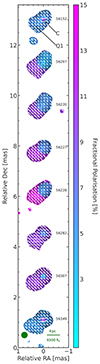 |
Fig. 1. Stokes I image (contours) and fractional polarisation geometrical model-fit (colour) of OJ 248 showcasing the epochs close in time to the MJD 56152–56349 (year: 2012−2013) γ-ray flare. The colour scale is linear, and the units are in percent. The dark green ellipse in the lower-left corner shows the common convolving circular beam size of 0.24 mas. The green bar (bottom right) corresponds to a projected distance of 6500 RS (Schwarzschild radius). Superimposed are the EVPAs (white sticks), showcasing the direction of the electric field and by extension that of the magnetic field (perpendicular). Their length is proportional to the fractional polarisation values. The lowest Stokes I contour cutoff at 5σI was implemented to only include high-S/N areas (with σI = 0.71 mJy/beam). The contour levels are at 0.25, 0.5, 1, 2, 4, 8, 16, 32, and 64% of the total intensity peak per epoch, the MJDs of which are denoted next to each observation. The core (C) and component Q1 are denoted in the first epoch. The EVPAs in C start out along the bulk jet flow (south-east direction). As the shock front progresses downstream, they exhibit a clear turn, becoming perpendicular to the bulk jet flow and aligned to the EVPAs in Q1. |
Summary of the component parameters
Simultaneously, the γ-ray light curve shown in the top panel of Fig. 2 exhibited a very bright flare, the prominence of which has not been repeated since. In parallel, a multi-band flare was also reported in the optical, near-IR, and millimetre radio bands by Carnerero et al. (2015), who also found an increase in the polarised flux and rotations in the optical EVPAs (although a clear trend was lacking). In the middle and bottom panels of Fig. 2 we overplot the radio wavelength EVPAs and flux density of C and Q1 during the flaring event. We can clearly observe that the γ-ray flare is accompanied by an EVPA rotation in the radio as well, which in turn is accompanied by a flux increase.
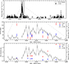 |
Fig. 2. OJ 248 component EVPAs and flux density, and the Fermi-LAT γ-ray light curve. In the top panel, the grey-shaded area marks the period in question, when the prominent γ-ray flare occurred. In the years since, the source has remained quiescent. The middle panel shows a zoomed-in view of the γ-ray flare time frame (grey-shaded area of the top panel), revealing a multi-peak profile. Additionally, the EVPAs in C (red) and Q1 (blue) were perpendicular to each other immediately before and after the γ-ray flare, but then rotated to be aligned during the flaring event. The bottom panel shows the same zoomed-in region but with the flux density of C denoted in red and that for Q1 in blue. We see an increasing trend in C. |
3. Discussion
The true nature of γ-ray flares is one of the fundamental open questions related to jet activity. To produce such a flare, a region of internal photons must be present for synchrotron self-Compton (Königl 1981) scattering (inverse Compton scattering) to occur: the so-called blazar zone (see e.g. Hovatta & Lindfors 2019, for a review). The exact location of this flare origin region with regard to the radio core observed with VLBI remains unclear. Both upstream (near the central engine) and downstream (extended jet) locations of the VLBI core have recently been proposed as the possible origin of flares, and this includes blazars (e.g. Rani et al. 2018) and, interestingly, radio galaxies (e.g. Paraschos et al. 2023), with the latter also showing evidence of a connection to jet feature ejections (Agudo 2013; Paraschos et al. 2022). Furthermore, jets could be transversely stratified, for example exhibiting a so-called spine-sheath geometry, where a fast inner plasma flow is surrounded by a slower moving one (Sol et al. 1989; Laing et al. 1996; Paraschos et al. 2024a). In this case, the blazar zone might be connected to either the spine or the sheath (see e.g. Blandford et al. 2019, for a review).
A common strategy of localising the blazar zone is to study the correlation between the onset and duration of a multi-band flare in different frequency bands. Interestingly, as discussed in Carnerero et al. (2015), the OJ 248 multi-band light curves recorded in γ-ray, optical, IR, and radio bands have exhibited a significant correlation over time when the source’s past main flaring events are taken into account. Such a manifestation is commonplace for blazars like OJ 248 (León-Tavares et al. 2011). The simultaneity of this multi-band flare and the activity in the jet dynamics found in our work strongly indicates a connection between them. A natural explanation of this phenomenon is that the blazar region is optically thin to radio wavelengths. The increase in the fractional polarisation in Q1 and the EVPAs’ rotation in C can be explained by a moving shock front, as reported, for example, in Liodakis et al. (2022). This shock front then appears to be ripping through a standing recollimation shock in the vicinity of the VLBI core (Daly & Marscher 1988), resulting in the observed peak multiplicity of the γ rays (see the middle and bottom panels of Fig. 2). Such activity has also been reported for the case of PKS 1510-089 in H.E.S.S. Collaboration (2021). We note with interest that a similar morphology has also been reported in other sources (e.g. Larionov et al. 2013; Liodakis et al. 2020).
We considered two alternative scenarios for the observed behaviour, namely a kink instability (Nalewajko 2017) and geometric effects. For the former we would expect a decrease in optical polarisation, which is not reported in Carnerero et al. (2015). A swinging nozzle model, in which abrupt changes to the viewing angle result in the flux density increase in all bands, has been proposed by Jorstad & Marscher (2004) to explain the latter scenario for OJ 248. The expected accompanying intra-night variability, however, has been lacking (as reported in Marchesini et al. 2016).
Another ansatz is the commonly invoked shock-in-jet model (Marscher & Gear 1985), which offers a convincing explanation for the increase in both the optical polarisation and fractional polarisation in the time frame of the γ-ray flare. In that case, the travelling shock front is expected to compress the magnetic field component perpendicular to the outflow and cause a rotation of the optical EVPAs (Blinov et al. 2018). However, similar to the cases of the radio sources 3C 454.3 (Liodakis et al. 2020) and S4 0954+65 (Kouch et al. 2025), in OJ 248 the EVPAs are directed perpendicular to the jet flow direction, which means that the magnetic field lines are parallel to it. Therefore, with the addition of the case of OJ 248 to the above two, there is now mounting evidence of the scenario described in Marscher et al. (2002). In that work, the authors postulate that ambient magnetic field lines parallel to the jet axis are possibly amplified by shearing processes or interactions with the surrounding medium. A passing shock front would then result in increased particle acceleration, which would lead to the observed geometry of the EVPAs in C. We propose that this description fits the observed phenomenology in our case: the shock propagates through and beyond C, which harbours an area of magnetic field lines parallel to the bulk jet flow. Particles are accelerated and then cool down, causing the γ-ray flare in this region of magnetic field lines streamlined to the jet axis. Furthermore, in this interpretation the magnetic field is not amplified (no compression to amplify the magnetic flux takes place), explaining the lower fractional polarisation values of C during the γ-ray flare. Finally, at the decay phase of the γ-ray flare, the magnetic field that the shock interacts with becomes more turbulent. This results in the compression of the field, providing order and restoring the EVPA orientation parallel to the bulk jet flow (see Kouch et al. 2025), which explains the observed rise in the fractional polarisation in C after the flare.
Overall, the rotation of the EVPAs in the central region (C) being simultaneous with the increase in the polarisation of the jet (Q1) is evidence in favour of the blazar region of OJ 248 being in the vicinity of the 43 GHz VLBI core. According to our present understanding of blazar jets (e.g. Marscher et al. 2008), this corresponds to an approximately parsec-scale distance to the central engine. Below, we also consider sub-parsec-scale distances for the blazar zone. Specifically, the dusty torus, a possible source of the seed electrons needed to cause the γ-ray flare (Saito et al. 2015; Ahnen et al. 2017), would be located too far upstream, close to the central engine. Similarly, a blazar region supported by photons from the broad line region, as suggested by Ghisellini & Madau (1996), would require the γ-ray flare to lag the optical one, which is not conclusively observed in Carnerero et al. (2015). Finally, if the blazar zone is located even farther downstream (a few parsecs away from the central engine), as indicated by the evolution of the jet seen in Fig. 1, the origin of the seed photons could be within a surrounding jet sheath (e.g. Attridge et al. 1999; MacDonald et al. 2015). This scenario, which particularly works for flat spectrum radio quasars such as OJ 248, has reportedly been able to produce the observed γ-ray flares (MacDonald et al. 2017), albeit in a suppressed magnetic field strength regime. In that case, we can also make a prediction about future γ-ray flares in the source based on the work presented by Blinov et al. (2021). The authors show that condensation rings within the jet sheath, surrounding the inner spine, can provide the necessary seed photons. Under these model assumptions, future γ-ray flares are predicted to exhibit a pattern similar to the one found here (i.e. multiple peaks).
4. Conclusions
In this work we investigated the connection between the polarisation properties of the OJ 248 jet and a prominent γ-ray flare detected in the same source. Our findings can be summarised as follows:
-
The OJ 248 jet exhibits remarkable morphological changes through the course of the flaring event, detected in γ-ray, optical, near-IR, and radio bands, as well as in polarised emission. Specifically, the VLBI fractional linear polarisation of its extended emission (component Q1) is heightened during the γ-ray outburst, while being in lower states immediately before and after. The EVPAs appear to also be affected; during the γ-ray flare they are perpendicular to the bulk jet flow, whereas before and after they are not.
-
This behaviour is consistent with a moving shock front travelling through a recollimation shock that causes the photons to be inverse Compton up-scattered and leads to γ-ray flare.
Our work showcases the importance of monitoring blazars with both VLBI and individual telescopes in multiple bands for gaining insights into their underlying physical mechanisms. Future higher-sensitivity instruments, such as the next-generation Very Large Array (ngVLA), will enable us to image fainter sources, such as OJ 248, in greater detail and thus leverage the possibilities that multi-messenger astronomy has ushered in.
Acknowledgments
We thank I. Liodakis and an anonymous referee for their valuable comments which greatly improved this manuscript and L. Debbrecht for the insightful discussions. This research is supported by the European Research Council advanced grant “M2FINDERS – Mapping Magnetic Fields with INterferometry Down to Event hoRizon Scales” (Grant No. 101018682). This study makes use of VLBA data from the VLBA-BU Blazar Monitoring Program (BEAM-ME and VLBA-BU-BLAZAR; http://www.bu.edu/blazars/BEAM-ME.html), funded by NASA through the Fermi Guest Investigator Program. The VLBA is an instrument of the National Radio Astronomy Observatory. The National Radio Astronomy Observatory is a facility of the National Science Foundation operated by Associated Universities, Inc. This research has made use of the NASA/IPAC Extragalactic Database (NED), which is operated by the Jet Propulsion Laboratory, California Institute of Technology, under contract with the National Aeronautics and Space Administration. This research has also made use of NASA’s Astrophysics Data System Bibliographic Services. Finally, this research made use of the following python packages: numpy (Harris et al. 2020), scipy (Virtanen et al. 2020), matplotlib (Hunter 2007), astropy (Astropy Collaboration 2013, 2018) and Uncertainties: a Python package for calculations with uncertainties.
References
- Abdo, A. A., Ackermann, M., Ajello, M., et al. 2010, ApJ, 716, 835 [NASA ADS] [CrossRef] [Google Scholar]
- Agudo, I. 2013, European Physical Journal Web of Conferences, 61, 04002 [NASA ADS] [CrossRef] [EDP Sciences] [Google Scholar]
- Ahnen, M. L., Ansoldi, S., Antonelli, L. A., et al. 2017, A&A, 603, A25 [NASA ADS] [CrossRef] [EDP Sciences] [Google Scholar]
- Ajello, M., Angioni, R., Axelsson, M., et al. 2020, ApJ, 892, 105 [NASA ADS] [CrossRef] [Google Scholar]
- Astropy Collaboration (Robitaille, T. P., et al.) 2013, A&A, 558, A33 [NASA ADS] [CrossRef] [EDP Sciences] [Google Scholar]
- Astropy Collaboration (Price-Whelan, A. M., et al.) 2018, AJ, 156, 123 [Google Scholar]
- Attridge, J. M., Roberts, D. H., & Wardle, J. F. C. 1999, ApJ, 518, L87 [NASA ADS] [CrossRef] [Google Scholar]
- Atwood, W. B., Abdo, A. A., Ackermann, M., et al. 2009, ApJ, 697, 1071 [CrossRef] [Google Scholar]
- Blandford, R., Meier, D., & Readhead, A. 2019, ARA&A, 57, 467 [NASA ADS] [CrossRef] [Google Scholar]
- Blinov, D., Pavlidou, V., Papadakis, I., et al. 2018, MNRAS, 474, 1296 [CrossRef] [Google Scholar]
- Blinov, D., Jorstad, S. G., Larionov, V. M., et al. 2021, MNRAS, 505, 4616 [NASA ADS] [CrossRef] [Google Scholar]
- Carnerero, M. I., Raiteri, C. M., Villata, M., et al. 2015, MNRAS, 450, 2677 [NASA ADS] [CrossRef] [Google Scholar]
- Chael, A. A., Johnson, M. D., Narayan, R., et al. 2016, ApJ, 829, 11 [Google Scholar]
- Daly, R. A., & Marscher, A. P. 1988, ApJ, 334, 539 [Google Scholar]
- Enya, K., Yoshii, Y., Kobayashi, Y., et al. 2002, ApJS, 141, 31 [NASA ADS] [CrossRef] [Google Scholar]
- Ghisellini, G., & Madau, P. 1996, MNRAS, 280, 67 [CrossRef] [Google Scholar]
- Harris, C. R., Millman, K. J., van der Walt, S. J., et al. 2020, Nature, 585, 357 [NASA ADS] [CrossRef] [Google Scholar]
- H.E.S.S. Collaboration (Abdalla, H., et al.) 2021, A&A, 648, A23 [NASA ADS] [CrossRef] [EDP Sciences] [Google Scholar]
- Hewett, P. C., & Wild, V. 2010, MNRAS, 405, 2302 [NASA ADS] [Google Scholar]
- Hovatta, T., & Lindfors, E. 2019, New Astron. Rev., 87, 101541P [Google Scholar]
- Hunter, J. D. 2007, Computing in Science& Engineering, 9, 90 [NASA ADS] [CrossRef] [Google Scholar]
- Jorstad, S. G., & Marscher, A. P. 2004, ApJ, 614, 615 [NASA ADS] [CrossRef] [Google Scholar]
- Jorstad, S. G., & Marscher, A. P. 2006, Astronomische Nachrichten, 327, 227 [NASA ADS] [CrossRef] [Google Scholar]
- Jorstad, S. G., Marscher, A. P., Mattox, J. R., et al. 2001, ApJ, 556, 738 [NASA ADS] [CrossRef] [Google Scholar]
- Jorstad, S. G., Marscher, A. P., Morozova, D. A., et al. 2017, ApJ, 846, 98 [Google Scholar]
- Königl, A. 1981, ApJ, 243, 700 [Google Scholar]
- Kouch, P. M., Liodakis, I., Fenu, F., et al. 2025, A&A, in press, https://doi.org/10.1051/0004-6361/202453127 [Google Scholar]
- Laing, R. A. 1996, in Energy Transport in Radio Galaxies and Quasars, eds. P. E. Hardee, A. H. Bridle, & J. A. Zensus, ASP Conf. Ser., 100, 241 [NASA ADS] [Google Scholar]
- Larionov, V. M., Jorstad, S. G., Marscher, A. P., et al. 2013, ApJ, 768, 40 [NASA ADS] [CrossRef] [Google Scholar]
- León-Tavares, J., Valtaoja, E., Tornikoski, M., Lähteenmäki, A., & Nieppola, E. 2011, A&A, 532, A146 [NASA ADS] [CrossRef] [EDP Sciences] [Google Scholar]
- Liodakis, I., Blinov, D., Jorstad, S. G., et al. 2020, ApJ, 902, 61 [NASA ADS] [CrossRef] [Google Scholar]
- Liodakis, I., Marscher, A. P., Agudo, I., et al. 2022, Nature, 611, 677 [CrossRef] [Google Scholar]
- MacDonald, N. R., Marscher, A. P., Jorstad, S. G., & Joshi, M. 2015, ApJ, 804, 111 [Google Scholar]
- MacDonald, N. R., Jorstad, S. G., & Marscher, A. P. 2017, ApJ, 850, 87 [Google Scholar]
- Marchesini, E. J., Andruchow, I., Cellone, S. A., et al. 2016, A&A, 591, A21 [NASA ADS] [CrossRef] [EDP Sciences] [Google Scholar]
- Marscher, A. P., & Broderick, J. J. 1983, AJ, 88, 759 [NASA ADS] [CrossRef] [Google Scholar]
- Marscher, A. P., & Gear, W. K. 1985, ApJ, 298, 114 [Google Scholar]
- Marscher, A. P., Jorstad, S. G., Mattox, J. R., & Wehrle, A. E. 2002, ApJ, 577, 85 [NASA ADS] [CrossRef] [Google Scholar]
- Marscher, A. P., Jorstad, S. G., D’Arcangelo, F. D., et al. 2008, Nature, 452, 966 [Google Scholar]
- McCall, C., Jermak, H. E., Steele, I. A., et al. 2024, MNRAS, 528, 4702 [NASA ADS] [CrossRef] [Google Scholar]
- Nalewajko, K. 2017, Galaxies, 5, 64 [Google Scholar]
- Paraschos, G. F., Krichbaum, T. P., Kim, J. Y., et al. 2022, A&A, 665, A1 [NASA ADS] [CrossRef] [EDP Sciences] [Google Scholar]
- Paraschos, G. F., Mpisketzis, V., Kim, J. Y., et al. 2023, A&A, 669, A32 [NASA ADS] [CrossRef] [EDP Sciences] [Google Scholar]
- Paraschos, G. F., Debbrecht, L. C., Kramer, J. A., et al. 2024a, A&A, 686, L5 [NASA ADS] [CrossRef] [EDP Sciences] [Google Scholar]
- Paraschos, G. F., Kim, J. Y., Wielgus, M., et al. 2024b, A&A, 682, L3 [NASA ADS] [CrossRef] [EDP Sciences] [Google Scholar]
- Paraschos, G. F., Wielgus, M., Benke, P., et al. 2024c, A&A, 687, L6 [NASA ADS] [CrossRef] [EDP Sciences] [Google Scholar]
- Piner, B. G., Bhattarai, D., Edwards, P. G., & Jones, D. L. 2006, ApJ, 640, 196 [NASA ADS] [CrossRef] [Google Scholar]
- Price, R., Gower, A. C., Hutchings, J. B., et al. 1993, ApJS, 86, 365 [NASA ADS] [CrossRef] [Google Scholar]
- Raiteri, C. M., Ghisellini, G., Villata, M., et al. 1998, A&AS, 127, 445 [NASA ADS] [CrossRef] [EDP Sciences] [Google Scholar]
- Rani, B., Jorstad, S. G., Marscher, A. P., et al. 2018, ApJ, 858, 80 [Google Scholar]
- Roelofs, F., Johnson, M. D., Chael, A., et al. 2023, ApJ, 957, L21 [NASA ADS] [CrossRef] [Google Scholar]
- Saito, S., Stawarz, Ł., Tanaka, Y. T., et al. 2015, ApJ, 809, 171 [Google Scholar]
- Sol, H., Pelletier, G., & Asseo, E. 1989, MNRAS, 237, 411 [NASA ADS] [Google Scholar]
- Villata, M., Raiteri, C. M., Ghisellini, G., et al. 1997, A&AS, 121, 119 [NASA ADS] [CrossRef] [EDP Sciences] [Google Scholar]
- Virtanen, P., Gommers, R., Oliphant, T. E., et al. 2020, Nature Methods, 17, 261 [CrossRef] [Google Scholar]
- Zhang, X., Xiong, D.-R., Gao, Q.-G., et al. 2024, MNRAS, 529, 3699 [NASA ADS] [CrossRef] [Google Scholar]
All Tables
All Figures
|
Fig. 1. Stokes I image (contours) and fractional polarisation geometrical model-fit (colour) of OJ 248 showcasing the epochs close in time to the MJD 56152–56349 (year: 2012−2013) γ-ray flare. The colour scale is linear, and the units are in percent. The dark green ellipse in the lower-left corner shows the common convolving circular beam size of 0.24 mas. The green bar (bottom right) corresponds to a projected distance of 6500 RS (Schwarzschild radius). Superimposed are the EVPAs (white sticks), showcasing the direction of the electric field and by extension that of the magnetic field (perpendicular). Their length is proportional to the fractional polarisation values. The lowest Stokes I contour cutoff at 5σI was implemented to only include high-S/N areas (with σI = 0.71 mJy/beam). The contour levels are at 0.25, 0.5, 1, 2, 4, 8, 16, 32, and 64% of the total intensity peak per epoch, the MJDs of which are denoted next to each observation. The core (C) and component Q1 are denoted in the first epoch. The EVPAs in C start out along the bulk jet flow (south-east direction). As the shock front progresses downstream, they exhibit a clear turn, becoming perpendicular to the bulk jet flow and aligned to the EVPAs in Q1. |
| In the text | |
|
Fig. 2. OJ 248 component EVPAs and flux density, and the Fermi-LAT γ-ray light curve. In the top panel, the grey-shaded area marks the period in question, when the prominent γ-ray flare occurred. In the years since, the source has remained quiescent. The middle panel shows a zoomed-in view of the γ-ray flare time frame (grey-shaded area of the top panel), revealing a multi-peak profile. Additionally, the EVPAs in C (red) and Q1 (blue) were perpendicular to each other immediately before and after the γ-ray flare, but then rotated to be aligned during the flaring event. The bottom panel shows the same zoomed-in region but with the flux density of C denoted in red and that for Q1 in blue. We see an increasing trend in C. |
| In the text | |
Current usage metrics show cumulative count of Article Views (full-text article views including HTML views, PDF and ePub downloads, according to the available data) and Abstracts Views on Vision4Press platform.
Data correspond to usage on the plateform after 2015. The current usage metrics is available 48-96 hours after online publication and is updated daily on week days.
Initial download of the metrics may take a while.