| Issue |
A&A
Volume 610, February 2018
|
|
|---|---|---|
| Article Number | A16 | |
| Number of page(s) | 17 | |
| Section | Interstellar and circumstellar matter | |
| DOI | https://doi.org/10.1051/0004-6361/201630271 | |
| Published online | 19 February 2018 | |
Dust models compatible with Planck intensity and polarization data in translucent lines of sight
1
Institut d’Astrophysique Spatiale, CNRS, Univ. Paris-Sud, Univ. Paris-Saclay,
Bât. 121,
91405 Orsay Cedex,
France
e-mail: This email address is being protected from spambots. You need JavaScript enabled to view it.
2
Laboratoire Univers et Particules de Montpellier, Université de Montpellier, CNRS/IN2P3, CC 72, Place Eugène Bataillon,
34095 Montpellier Cedex 5,
France
3
LERMA, Observatoire de Paris, PSL Research University, CNRS, Sorbonne Universités, UPMC Univ. Paris 06,
École normale supérieure,
75005 Paris,
France
4
CNRS, IRAP,
9 Av. colonel Roche,
BP 44346,
31028 Toulouse Cedex 4,
France
Received:
16
December
2016
Accepted:
24
October
2017
Abstract
Context. Current dust models are challenged by the dust properties inferred from the analysis of Planck observations in total and polarized emission.
Aims. We propose new dust models compatible with polarized and unpolarized data in extinction and emission for translucent lines of sight (0.5 < AV < 2.5).
Methods. We amended the DustEM tool to model polarized extinction and emission. We fit the spectral dependence of the mean extinction, polarized extinction, total and polarized spectral energy distributions (SEDs) with polycyclic aromatic hydrocarbons, astrosilicate and amorphous carbon (a-C) grains. The astrosilicate population is aligned along the magnetic field lines, while the a-C population may be aligned or not.
Results. With their current optical properties, oblate astrosilicate grains are not emissive enough to reproduce the emission to extinction polarization ratio P353∕pV derived with Planck data. Successful models are those using prolate astrosilicate grains with an elongation a∕b = 3 and an inclusion of 20% porosity. The spectral dependence of the polarized SED is steeper in our models than in the data. Models perform slightly better when a-C grains are aligned. A small (6%) volume inclusion of a-C in the astrosilicate matrix removes the need for porosity and perfect grain alignment, and improves the fit to the polarized SED.
Conclusions. Dust models based on astrosilicates can be reconciled with Planck data by adapting the shape of grains and adding inclusions of porosity or a-C in the astrosilicate matrix.
Key words: polarization – dust, extinction – submillimeter: ISM – methods: numerical
© ESO 2018
1 Introduction
Dust emission is an important tracer of the interstellar medium (ISM), be it Galactic or extra-Galactic; it traces the star formation activity and provides estimates of the gas mass (Hildebrand 1983). Dust polarized emission allows one to measure the orientation of the magnetic field and estimate its strength (Chandrasekhar & Fermi 1953). Dust emission is a nuisance for the study of the primorial physics of the universe (CMB B-Modes, BICEP2/Keck and Planck Collaborations 2015; Planck Collaboration Int. L 2017) or of external galaxies, as no field in our galaxy can be considered as free of dust. The characterization of dust properties and their variations through the ISM is therefore an important goal for both galactic physics and cosmology.
Dust properties vary from one line of sight to the other (Martin et al. 2012), tracing the proper history of interstellar matter in its lifecycle (Jones et al. 2013; Zhukovska et al. 2016). These variations are well characterized in extinction in the diffuse ISM (Fitzpatrick & Massa 2007). The Planck mission, providing a full-sky survey of the dust total and polarized emission in the submillimeter, has greatly improved our knowledge of dust optical properties in emission, polarized and unpolarized, and allowed us to quantify their variations through the diffuse ISM (Planck Collaboration XI 2014; Planck Collaboration Int. XXII 2015; Fanciullo et al. 2015; Planck Collaboration XXIX 2016). Lately, the balloon-borne observations by BLASTPol characterized the variations of dust polarization properties in higher-density regions like the Vela C cloud (Fissel et al. 2016; Gandilo et al. 2016; Santos et al. 2017; Ashton et al. 2017).
The growing amount of available and upcoming dust observations in emission, extinction, and polarization on the same lines of sight offers the possibility of a consistent analysis of the full spectrum of dust observables. Differences in, for example, beam size and path length probed along the line of sight must be carefully taken into account in the line of sight selection and correlation analysis phases. If those effects are properly taken into account, one can provide new constraints for dust models (e.g., Planck Collaboration Int. XXI 2015). At high column densities, radiation transfer effects also appear, an effect which can only be solved with a dedicated three-dimensional (3D) model (Ysard et al. 2012; Reissl et al. 2016).
Existing dust models (e.g., Zubko et al. 2004; Draine & Li 2007; Draine & Fraisse 2009; Compiègne et al. 2011; Jones et al. 2013; Siebenmorgen et al. 2014) are calibrated on the mean extinction curve and the pre-Planck mean spectral energy distribution (SED) observed at high Galactic latitude. They are consistent with cosmic abundances. Some of them (Draine & Fraisse 2009; Siebenmorgen et al. 2014) also comply to the mean spectral dependence of polarization in the optical (Serkowski et al. 1975). These models now need to be updated utilizing the new observational constraints extracted from Planck observations of dust polarized and unpolarized emission. Planck Collaboration XXIX (2016) demonstrated that the Draine & Li (2007) dust model is not emissive enough per unit extinction, by a factor ~ 2, to explain the observed dust SED per AV at high Galactic latitude. A similar factor was found independently by Dalcanton et al. (2015) when comparing dust extinction and emission in M31. In Planck Collaboration Int. XXI (2015, hereafter Paper I), we showed that the Draine & Fraisse (2009) dust model, adapted from Draine & Li (2007), does not emit enough polarized emission at 353 GHz, by a factor 2.5, compared to its counterpart in polarization in the optical toward stars on translucent lines of sight (0 < AV < 2.5). These new observational constraints all point to the need for more strongly emissive dust grains, especially for the silicate component that is known to be aligned with the magnetic field and therefore responsible for much, and possibly all, of the polarization of dust emission and extinction.
The Jones et al. (2013) dust model, which was built upon theoretical considerations and laboratory data, includes strongly emissive core-mantle grains that can successfully reproduce the dust SED observed by Planck in the diffuse ISM (Fanciullo et al. 2015). This model is part of a more global renewal of our approach of grain physics (the THEMIS framework, see Jones et al. 2017), which attempts to provide a consistent set of physically motivated predictions for observed variations in dust emission, extinction and scattering from the diffuse to the dense ISM phases (Köhler et al. 2015; Ysard et al. 2015, 2016; Jones et al. 2016). Defining and calculating the properties of THEMIS grains for polarization is a difficult andlong task, owing to their complex structure and composition. This ongoing work will be published elsewhere.
There is a need for a simple dust model that fits Planck polarized and unpolarized data. In this paper, we amend the Compiègne et al. (2011) model for polarization. The shape and composition of dust grains are adapted to fit observational constraints in extinction and emission. Such a model can help to analyze polarization data and disentangle between the various physical effects (magnetic field structure, dust alignment, and dust evolution) that contribute to the observed variations of dust polarization properties (Fanciullo et al. 2017).
Our paper is structured as follows: Sect. 2 presents the way polarization is implemented in our dust modeling tool, DustEM. Section 3 details the calculation of the grain absorption and scattering cross-sections for spheroidal grains, and their averaging over the grain spinning dynamics. Section 4 presents the observational data to be fitted by our models. In Sect. 5, we detail our dust populations and the methods by which we can adapt the shape and porosity of the grains to fit Planck data. Section 6 presents four models compatible with Planck polarized and unpolarized data, with or without carbon grains aligned, and with porous or composite silicate grains. A short discussion of our resultsfollows in Sect. 7, and we conclude with a summary of our results in Sect. 8.
2 Modeling dust polarization with the DustEM tool
DustEM1 (Compiègne et al. 2011) is a fortran code to physically model dust emission and extinction. Combined with its IDL wrapper2, it can also fit extinction curves and SEDs. We have amended the DustEM and wrapper codes to also model and fit polarization in extinction and in emission.
2.1 Modeling of dust alignment in DustEM
The polarization of starlight results from the dichroic extinction of light by interstellar dust grains, which are aspherical and aligned along the magnetic field lines (Davis & Greenstein 1951). The spectral dependence of polarization in the optical shows that while large (a ≥ 0.1 μm) grains are preferentially aligned, small grains (a ≪ 0.1 μm) are not (Kim & Martin 1995). Dust emission is also polarized (Stein 1966), with a direction of polarization that is orthogonal to that in extinction.
Interstellar grains behave like spinning tops, gyrating around their axis of maximal inertia. This spin axis precesses around magnetic field lines due to the magnetic moment of the grains. Two main physical processes have been proposed to explain the alignment of grains in the ISM (for a recent review on dust alignment, see Andersson et al. 2015): by magnetic dissipation (Davis & Greenstein 1951), or by radiative torques (RATs, Draine & Weingartner 1996, 1997; Lazarian & Hoang 2007). A recent revision of the RAT paradigm shows that magnetic dissipation and radiative torques are both necessary to explain to level of polarization observed in the diffuse ISM (Hoang & Lazarian 2016).
A physical alignment model must predict the grain dynamics around magnetic field lines as a function of the grain size and of the physical conditions in the environment. This is the case for the alignment process by magnetic dissipation (Davis & Greenstein 1951; Siebenmorgen et al. 2014), but not yet for the RATs, though this is a work in progress (Hoang & Lazarian 2016).
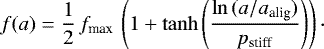
The DustEM tool uses a parametric model for dust alignment. For each grain population, grains of a given size a are divided into two components: the grains of the first component are aligned with the magnetic field, while those of the second component have a random orientation and are therefore not polarizing. The fraction of mass of the aligned component, f(a), is a function of the grain radius through three parameters fmax, aalig and pstiff :
 (1)
(1)
The fractionf(a) increases with a from 0 to fmax, with a transition at a = aalig characterized by a stiffness pstiff. For a stiffness pstiff = 1, f(aalig∕2) = 0.2 and f(2 aalig) = 0.8. This expression, which gives satisfactory results for all our purposes, also mimics the size dependence of grain alignment expected from RATs (Hoang & Lazarian 2016) or from superparamagnetic Davis-Greenstein alignment (Voshchinnikov et al. 2016).
2.2 Polarization observables with DustEM
The polarization properties of grains do not only depend on the dust alignment efficiency, but also on the magnetic field orientation and its variations along the line of sight. In this article, we model the highest polarization fraction observed in extinction on translucent lines of sight, which most probably corresponds to a situation where the magnetic field B lays in the plane of the sky and is uniform along the line of sight (Martin 2007). To remain general however, we note Bpos the projection of B onto the plane of the sky.
For each grain population, DustEM uses tabulated values in size a and wavelength λ of the grain absorption, Cabs, scattering, Csca and extinction, Cext = Cabs + Csca, cross-sections. Different tables are needed; for the unaligned component, DustEM uses the cross-sections C<abs>, C<sca> and C<ext> calculated for grains in random orientation; and for the aligned component, cross-sections were calculated for two directions of the E component of an incident electromagnetic wave:
- 1.
C1, abs, C1, sca and C1, ext: E along Bpos,
- 2.
C2, abs, C2, sca and C2, ext: E perpendicular to Bpos.
The detailed calculation of those cross-sections is described in Sect. 3. For simplicity, we assumed in this article that the grains of the aligned component are in perfect spinning alignment (that is, that the grain spin axis remains fixed along B ), though our detailed calculations of the grain cross-sections would allow for any grain dynamics.
The dust total polarization cross-section is the sum of all the contributions of grain size ai over all grain populations j. This yields
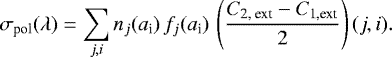 (2)
(2)
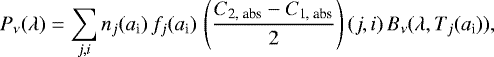
The total polarized intensity Pν(λ) is:
 (3)
(3)
where Tj(ai) is the temperature of a grain of size ai from population j, as calculated by DustEM, and Bν(λ, T) is the associated Planck function.
2.3 Extinction and emission
When dust grains are aspherical, their emission and extinction cross-sections depend in principle on the magnetic field orientation and grain alignment efficiency (e.g., Hong & Greenberg 1980; Das et al. 2010). However, when the spectral dependence in extinction and in emission are mean values averaged out over many lines of sight at all longitudes, as is the case in this paper (Sect. 4), dust grains have no preferred orientation. We therefore assume that grains are all in random orientation for the fitting of the extinction and emission curves:

3 Calculation of the cross-sections of spinning spheroidal grains
Unlike polarization by scattering, which can be produced by non-aligned spherical grains, grains must be both aspherical and at least partially aligned to produce polarization in extinction and in emission.
3.1 Grain shape
From a modeling point of view, the most simple non-spherical shape is the spheroid, which is obtained by rotating an ellipse around one of its axes. If the axis of revolution of the grain is its minor axis, the grain is said to be oblate; if the axis of revolution is its major axis, the grain is said to be prolate.
We note  the axis of revolution of the grain, of length 2a. The two other axes have a length 2b. We define the grain axis ratio ϵ = b∕a: ϵ > 1 for oblate grains and ϵ < 1 for prolate grains. The radius of the sphere that has the same volume as this spheroid is
 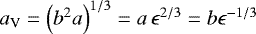 .
.
To help comparing the properties of oblate and prolate grains, an oblate grain with ϵ = 2 and a prolate grain with ϵ = 1∕2 will be said to have the same elongation, equal to 2.
3.2 Grain cross-sections for any inclination angle ψ
In the common view, grains are similar to spinning tops: they spin around their minor axis, which is precessing around magnetic field lines with a nutation angle that can vary with time (Davis & Greenstein 1951). The grain cross-sections must therefore be calculated for any orientation of the grain with respect to the line of sight. For symmetry reasons, the grain cross-sections will only depend on the inclination angle, ψ, of the grain symmetry axis  with respectto the line of sight.
Let us consider a spheroidal grain of equivalent radius aV and axis ratio ϵ, built in a material that has a complex refractive index m = n + ik at a given wavelength λ. Following the approach of Das et al. (2010), we calculate the grain cross-sections for 31 values of ψ from 0 to 90° in steps of 3degrees. To that end, we use the T-MATRIX code in its extended precision version amplq.lp.f. This is a numerical adaptation of the Extended Boundary Condition Method (Waterman 1971) for non-spherical particles in a fixed orientation (Mishchenko 2000). The code proceeds in two steps: 1) it calculates the T matrix for this particular spheroidal grain characterized by aV, ϵ and m. This is the longest step; 2) knowing T, the code can derive the 2 × 2 complex amplitude matrix S for any orientation of the grain in the laboratory frame (as specified by two Euler angles α and β), any direction (θi, ϕi) of the incident beam, and any direction (θs, ϕs) of the scattered beam. This last step, which allows for the calculation of the grain cross-sections, is computationally fast.
Let us detail this second step. We calculate the grain cross-sections for two different orientations of the incident polarization, with either the E or H component of the incident electromagnetic wave in the plane containing  and the line of sight (Hong & Greenberg 1980). The extinction cross-sections can be derived from the complex extinction matrix S, that is, the amplitude matrix when the incident and scattered beams are directed toward the observer (Eqs. (31) and (33) from Mishchenko et al. 2000):

where ℑ is the imaginary part of the complex.
The grain scattering cross-section Csca is obtained by averaging some components of S over all directions (θs, ϕs) of the scattered beams (Mishchenko et al. 2000):

The scattering directions are extracted from a HEALPix3 map with Nside = 8 (Gorski et al. 2005). This provides the zenith and azimuth angles (θs, ϕs) for N = 768 directions uniformly distributed in space; a sampling good enough for our calculations.
The absorption cross-sections for E and H polarizations are given by:
 (10)
(10)
3.3 Extrapolation in the geometric limit
The T-MATRIX fortran code (Mishchenko 2000) fails in the ultraviolet for elongated particles with large aV ∕λ ratios4. The calculation time also increases rapidly with aV∕λ. To limit the calculation time, we stop our calculations at aV∕λ = 4 for all grains. In case the code fails, we note λ0 the shortest wavelength for which the calculation was still successful. To estimate the absorption and scattering cross-sections at wavelengths shorter than λ0, we interpolate between the value calculated at λ = λ0 and the value predicted by geometric optics.
In geometric optics (aV ≫ λ), the grain geometrical cross-section, Cgeo, is a function ofthe inclination angle ψ between the grain’s axis of symmetry and the line of sight (Binggeli 1980):
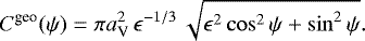 (11)
(11)
To calculatethe absorption and scattering cross-section in the geometric limit, we follow Min et al. (2003) and assume that the grain albedois independent of the grain shape:

where  is the grain albedo of a sphere of radius aV, as calculated by the Mie Theory.
We finally interpolate the absorption and scattering cross-sections between λ0 and the Lyman continuum using the linear expression:
 (14)
(14)
Resulting cross-sections are presented in Sect. 5.4.
3.4 Averaging cross-sections over the grain spinning dynamics
The grain cross-sections must be averaged over the grain dynamics around magnetic field lines. As this article aims at modeling the highest polarization fraction observed in extinction and in emission, it is reasonable to assume that this corresponds to the case of optimal alignment, that is, grains in perfect spinning alignment. Therefore, we ignore the possible nutation and precession of the grain around magnetic field lines, and assume that the spin axis of the grain remains constantly aligned with B.
The spinning of the grain can be ignored for oblate grains because the spin axis, which is also the axis of symmetry, remains parallel to the magnetic field. With the notations from Sects. 2.2 and 3.2, this yields:

This is not the case for prolate grains for which the cross-sections must be integrated over the grain spinning dynamics around its minor axis. For prolate grains, the grain symmetry axis is perpendicular to the magnetic field during its spinning. Therefore:

Appendix B gives the expressions for C1 and C2 when the magnetic field is inclined with respect to the plane of the sky, still with perfect spinning alignment.
3.5 Grain absorption and scattering cross-sections for random orientations
Not all grains are aligned with the magnetic field lines. For these grains, the absorption and scattering cross-sections must be calculated in a random orientation. Moreover, grains even perfectly aligned with the magnetic field have no preferred orientation with respect to the photons of the interstellar radiation field (ISRF) that heat them. The grain absorption cross-section used to derive the dust temperature must therefore be calculated with no preferred orientation.
For each direction k of the N = 768 directions provided by the HEALPix Nside = 8 map, we calculate the inclination angle ψk of the grain’s axis of symmetry with the line of sight and interpolate the E and H components of the grain absorption cross-section on our library of 31 values for ψ between 0 and 90° (see Sect. 3.2).
The resulting cross-sections for random orientation are given by:
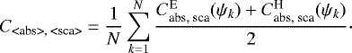 (19)
(19)
3.6 Absorption, scattering, and extinction coefficients Q
From the calculated grain cross-sections we define the grain absorption, scattering, extinction, and polarization coefficients, Qabs, Qsca, Qext, Qpol, respectively,as the ratio of the corresponding cross-section to the cross-section of the volume of the equivalent sphere  .
.
4 Observational constraints for dust in translucent lines of sight
The spectral data usually used to constrain dust model parameters do not all relate consistently to a specific interstellar environment. On the one hand, the extinction curves of Mathis (1990) and Fitzpatrick (1999), the spectral dependence of the starlight polarization degree (Serkowski et al. 1975), and the amount of extinction per H, AV ∕NH, (Bohlin et al. 1978; Rachford et al. 2009), have been measured toward stars at low Galactic latitude and moderate interstellar extinction (AV ~ 1). On the other hand, the normalization per H, or per AV, of the dust SED has only been calculated at high Galactic latitude and low extinction through the correlation with the HI 21-cm emission (Boulanger et al. 1996; Planck Collaboration Int. XVII 2014; Planck Collaboration XI 2014) or with the extinction to QSOs (Planck Collaboration XXIX 2016). For the moment, we lack the spectral information at high Galactic latitude in extinction and in polarization by extinction to present a consistent dust model for this particular ISM.
In Paper I, we selected 206 suitable lines of sight to stars, at all Galactic longitudes and low Galactic latitude (|b| ≤ 30°), to correlate the Planck polarization measures at 353 GHz with starlight polarization in the optical taken from the compilation of polarization catalogs of Heiles (2000). The V band extinction toward those stars spanned a range 0.5–2.5 mag, with a mean of 1.5 mag. These lines of sight, which are not diffuse, should rather be called translucent. They do not always cross a translucent cloud however (Rachford et al. 2009). For these lines of sight, we found tight correlations between the starlight polarization degree, pV, and the polarized intensity at 353 GHz, P353, as well as between the polarization fraction in extinction, pV∕τV, and that in emission at 353 GHz, P353∕I353. Paper I provides the emission to extinction ratios needed to normalize the SEDs of polarized (resp. unpolarized) intensity in units of polarized (resp. unpolarized) extinction:
- 1.
RP∕p = P353∕pV = [5.4 ± 0.5] MJysr−1,
- 2.
Rs/V = (P353∕I353)∕(pV∕τV) = 4.2 ± 0.5,
- 3.
and consequently, I353∕AV = [1.2 ± 0.1] MJysr−1.
4.1 Extinction τ(λ)
As in Compiègne et al. (2011), we use the extinction curve τ(λ) of Fitzpatrick (1999) for the ultraviolet (UV) and optical (assuming RV = 3.1), and that of Mathis (1990) for the near-infrared (NIR) down to 4 μm. The normalization of the total extinction τ(λ) per H, needed to compare the mass of dust used in the model with cosmic abundances, is done using NH ∕AV = 1.87 × 1021 cm−2 (Rachford et al. 2009).
4.2 Optical and near-infrared polarization degree p(λ)
The UV-to-NIR polarization curve5, p(λ), is the traditional Serkowski et al. (1975) curve, reviewed by Draine & Allaf-Akbari (2006) with λmax = 0.55 μm and K = 0.92
 (20)
(20)
followed by a power-law extension from λ = 1.39 μm up to 4 μm with an index of − 1.7 (Martin et al. 1992; Draine & Fraisse 2009). The value of p(λ) at λ = λmax, pmax, is set using the maximal observed starlight polarization degree in the optical per unit reddening, pV ∕E(B − V ) = 9% (Serkowski et al. 1975). This yields pV∕τV = 3.15% or equivalently pV∕AV = 2.9%.
4.3 Dust total emission Iν(λ)
We derive a new reference SED, Iν(λ), for the translucent lines of sight studied in Paper I. We use the High Frequency Instrument (HFI) Planck maps in their PR2 release available from the Planck Legacy Archive (Planck Collaboration VIII 2016), together with IRIS and DIRBE maps (Miville-Deschênes & Lagache 2005; Hauser et al. 1998). Deriving a mean SED per H in translucent lines of sight is a difficult task. In this range of column densities, the 21-cm HI emission is not a good proxy for the total gas column density because of the presence of undetected molecular hydrogen. Instead, we use the 857 GHz Planck channel, which has the best signal-to-noise ratio (S/N) (instrumental as well as generated by CIB fluctuations), to obtain a SED normalized at 857 GHz. We compute the linear regression of each dust emission channel with the Planck intensity at 857 GHz using the regress IDL code, for those lines of sight with 5 < I857 < 20 MJysr−1, corresponding to the range 0.5–2.5 mag of V band extinction studied in Paper I. Cosmic microwave background (CMB) and cosmic infrared background (CIB) fluctuations, which are uncorrelated with dust emission, are removed by the correlation analysis, and integrated in the derived statistical uncertainty. The resulting SED, which is normalized at 857 GHz, is presented in Table 1, with its uncertainty σI (λ) extracted from the correlation.
The normalized SED is converted into a SED per unit extinction Iν (λ)∕AV using the ratio I353 ∕AV = (1.2 ± 0.1) MJysr−1 of Paper I. The uncertainty of 0.1 MJysr−1, being systematic, is not included in our error bars. The resulting SED is presented in Fig. 1, together with the mean SED from Planck Collaboration XXIX (2016) characteristic of the high Galactic latitude ISM, and the Compiègne et al. (2011) model SED. All SEDs look very similar in shape, especially in the submillimeter, but the normalization per unit extinction emphasizes systematic differences. At high Galactic latitude, I353 ∕AV = 0.9 ± 0.1MJysr−1 (Planck Collaboration XXIX 2016), a value which is well accounted for by the Jones et al. (2013) dust model, but not by the Compiègne et al. (2011) and Draine & Li (2007) dust models (Fanciullo et al. 2015). The present SED, with its higher emission-to-extinction ratio, I353 ∕AV = 1.2 MJysr−1, characteristic of translucent lines of sight at low Galactic latitude, can neither be reproduced by the Compiègne et al. (2011), nor by the Jones et al. (2013) or Draine & Li (2007) dust models, even taking into account the systematic error on I353 ∕AV of 0.1 MJysr−1.
Finally, Iν(λ)∕AV is converted into an emission per H using NH ∕AV = 1.87 × 1021 cm−2 (Rachford et al. 2009).
Mean dust SED per unit I857 for the lines of sight with 5 < I857 < 20 MJysr−1.
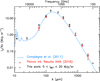 |
Fig. 1 (Black) New reference SED for translucent lines of sight (5 < I857 < 20 MJysr−1), converted into a SED per AV assuming I353∕AV = 1.2 MJysr−1. Errors bars include statistical and gain uncertainties, but not the systematic uncertainty of 0.1 MJysr−1 on I353 ∕AV from Paper I (see Sect. 4.3). (Red) SED measured in the high Galactic latitude ISM by Planck Collaboration XXIX (2016). (Blue) Dust SED from the Compiègne et al. (2011) model. |
4.4 Polarized SED Pν(λ)
The wavelength dependence of polarized emission was characterized with Planck HFI data at intermediate, not low, Galactic latitude (Planck Collaboration Int. XXII 2015). Variations in the spectral dependence of Iν (λ) are observed between the diffuse ISM and dense clouds (Ysard et al. 2013), and are therefore expected in Pν (λ). In the submillimeter, both polarized and unpolarized emission are dominated by the thermal emission of large grains. It is therefore not unreasonable to assume that the ratio of these two quantities, P∕I, may be less affected by these variations. As a proxy, we therefore assume that the mean wavelength dependence of the dust polarization fraction P∕I (Tables 3 and 6 from Planck Collaboration Int. XXII 2015) is the same at intermediate and low Galactic latitude.
From the wavelength dependence of P∕I, we obtain Pν(λ), the dust polarized emission per H, by multiplying P∕I by the Iν(λ) from Sect. 4.3. From the value of Rs/V = (P353∕I353)∕(pV∕τV = 4.2 (Sect. 4) and pV∕τV = 3.15% (Sect. 4.2), we infer a maximal polarization fraction P353∕I353 = 13%. This is indeed close to the maximal observed polarization fraction in emission at these column densities (Planck Collaboration Int. XIX 2015, see their Fig. 19 for NH ~ 3 × 1021 cm−2, corresponding to our mean AV ~ 1.5).
4.5 Error bars and fitting procedure
We use the DustEM wrapper based on MPFIT (Markwardt 2009) to simultaneously fit four curves: the extinction curve τ(λ), the polarization curve in extinction p(λ), the total SED Iν(λ), and the polarized SED in emission, Pν(λ), which have nτ = 43, np = 22, nI = 12 and nP = 4 data points, respectively, and hence a total of n = 81 data points.
Error bars are set uniformly to 10% of the data for τ(λ) and p(λ), except at the V band where it is set at 1% because Iν(λ) and Pν(λ) are normalized per AV and pV, respectively. For Iν(λ), we use the uncertainties derived from our correlation analysis (Sect. 4.3), with a lower limit of 1% set to avoid excessive weight from 353 down to 100 GHz. Signal-to-noise ratio for Pν (λ) is that from Planck Collaboration Int. XXII (2015).
We choose to give equal weights to each curve i in the fit, that is, we decide that the fit is equally constrained by each of the four curves. However, for a given curve, data points with a better S/N (e.g., from Planck) will still have a stronger weight during the fit. To obtain this behaviour, the χ2 driving the fit is the pondered sum of the four individual  of each curve:

where Mi,j, Di,j and σi,j are the model value, the data value and the uncertainty of the data point j from the curve i (ni data points), respectively. With this definition,  is independent of ni. The resulting fit will neither depend on the number of data points, nor on the particular value of the S/N (10% here), chosen for p(λ) and τ(λ).
5 Dust modeling
The submillimeter dust emission probed by Planck HFI, the one we want to model here, is dominated by the emission of large grains (~ 0.1 μm), which are also responsible for the polarization of dust extinction and emission. The UV portion of the extinction and polarization curves, together with the mid-infrared emission, are of secondary importance in this article. We therefore decide to simplify the Compiègne et al. (2011) description of the grain size distributions in order to limit the number of free parameters and allow for an easier and clearer study of the influence of relevant parameters.
5.1 Dust populations
As the thermal emission of polycyclic aromatic hydrocarbons (PAHs) is not central to this work, we change the modeling of PAHs in Compiègne et al. (2011) from two populations, neutral and positively charged, to one single, neutral, population. The size distribution of the two populations of large grains, amorphous carbon (hereafter a-C), and astrosilicate, which were modeled in Compiègne et al. (2011) by power laws with an exponential decay, are now replaced by power laws. The Very Small Grains (VSG) population is removed and incorporated in the power-law description of the large carbon grain population. Our model therefore entails only three distinct dust populations:
- 1.
a population of PAHs, with a log-normal size distribution defined by its adjustable total mass mPAH, and its fixed mean radius aPAH = 0.5 nm and width σPAH = 0.4 (Draine & Li 2007);
- 2.
a population of a-C grains (ρ = 1.81 g cm−3), with a power-law size distribution; and
- 3.
a population of astrosilicate grains (ρ = 3.5 g cm−3), with a power-law size distribution.
PAHs do not generally produce a significant polarization feature in the UV, except on two lines of sight (Clayton et al. 1992; Wolff et al. 1993, 1997; Hoang et al. 2013). We therefore assume that PAHs are not aligned.
The optical properties of the a-C population (the BE sample from Zubko et al. 1996, obtained through the burning of benzene in air) were not measured beyond 2 mm, and begin to deviate from a power-law at λ = 1 mm. As in Compiègne et al. (2011), we extrapolate cross-sections from 800 μm to 1 cm with a power-law fitted in the range 800–1000 μm. We also present and discuss in Appendix A the strange behavior of these optical properties when they are applied to small grains in the UV (λ < 0.15 μm). This has some implications on the size distribution of small carbon grains, but is of minor importance for this article.
The astrosilicates that were used in Compiègne et al. (2011) results from the modification by Li & Draine (2001, hereafter LD01) of the traditional Draine & Lee (1984) astrosilicates. Li & Draine (2001) decreased the spectral index of astrosilicates from β = 2 to β = 1.6 for 800 μm < λ < 1 cm to increase the emissivity of astrosilicate grains. Such an adhoc modification of the optical properties of astrosilicates is not needed to fit FIR and submm data when one uses amorphous carbon instead of graphite (Jones et al. 2013). We therefore prefer to use the unmodified pre-2001 description of astrosilicates (Weingartner & Draine 2001, hereafter WD01) with its uniform far-infrared and submillimeter spectral index β = 2.0. Still, one of our models (model B) will use the LD01 modified astrosilicates for the purpose of comparison.
5.2 Radiation field intensity G0
The mean radiation field intensity on translucent lines of sight may differ from the one in the diffuse ISM.To derive an estimate for the radiation field intensity, namely its scaling factor G0, we proposed a method in Fanciullo et al. (2015) which combines the dust SED with a measure of the dust extinction in the V band, that detail below. The dust radiance,  , is the total energy (unit W m−2 sr−1) emitted by dust at thermal equilibrium.
  can be calculated by direct numerical integration of the dust SED, or from the observed temperature Tobs, spectral index βobs, and optical depth at the frequency ν0 = 353 GHz obtained through a fit to the SED (Planck Collaboration XI 2014):
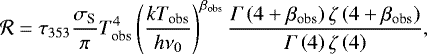 (24)
(24)
where σS is the Stefan-Boltzmann constant, k is the Boltzmann constant, h is the Planck constant, and Γ and ζ are the Gamma and Riemann zeta functions, respectively,
Through the conservation of the energy,  is also equal to the radiative energy absorbed by the same dust grains on the line of sight, and is therefore proportional, for a uniform medium in a uniform and anistropic radiation field, to G0, to the total amount of dust on the line of sight estimated from the dust extinction AV in the V band6, and to the dust albedo
  :
:
 (25)
(25)
Following our approach in Fanciullo et al. (2015), we use the radiance per unit extinction,  , as a proxy for the radiation field intensity. For the total V band extinction on the line of sight, we use the cumulative reddening map,
  , based on Pan-STARRS 1 and 2MASS photometry toward a few hundred million stars (Green et al. 2015). For the radiance map, we use improved versions of Planck maps of the dust temperature Tobs, spectral index βobs, opacity at 353 GHz τ353, where the contamination of galactic dust thermal emission by CIB anisotropies has been removed (Planck Collaboration XLVIII 2016). The radiance map derived from Eq. (24) is then converted to a reddening,
  , by correlation with the observed interstellar reddening to 2 00 000 QSOs, as per Planck Collaboration XI (2014).
If we make the reasonable assumption that the average radiation field toward QSOs is the ISRF (G0 = 1), we can define the following estimator of G0:
 (26)
(26)
By construction, Ĝ0 should be close to 1 in the diffuse ISM if the Planck  and Pan-STARRS
  maps agree. This comparison was done in Green et al. (2015) for the Planck Collaboration XI (2014) radiance map: a good agreement was found betwen
  and
and  below a reddening of 0.3. This can again be checked for our improved radiance map by controlling the value of Ĝ 0 on lines of sight through the diffuse ISM.
Figure 2 presents how the dust temperature Tobs correlates with our estimator Ĝ0. Color indicates the mean reddening, as derived from the dust optical depth τ353 at 353 GHz. The high latitude diffuse ISM (with an equivalent reddening lower than 0.02) has a Ĝ 0 close to 1, as expected. Most of the lines of sight to the 206 stars from Paper I also fall around Ĝ 0 = 1. Only two lines of sight from our sample cross dense clouds (shown in red, with an equivalent reddening of ~ 1). The blue line indicates the expected trend  , assuming that the dust optical properties were uniform in the ISM (β = 1.6) and fixing T = 18.5 K for
  . Our sample follows this trend line: some lines of sight probe colder dust, some other warmer dust (up to Ĝ 0 ≃ 4–5 and Tobs ≃ 23–24 K), but the mean value for the sample is not significantly different from that in the diffuse ISM. Furthermore, we showed in Paper I that the dust properties on those lines of sight with warmer dust did not differ signficantly from the rest of the sample.
We therefore decide to fix the radiation field intensity in our models to its reference value, G0 = 1, as in Compiègne et al. (2011).
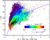 |
Fig. 2 Planck dust temperature, T, as a functionof our estimate for the radiation field intensity, |

5.3 Calculation of the refractive indices for porous and composite grains
The introduction of porosity in a grain tends to greatly increase the far-infrared and submillimeter emissivity of grains while only slightly decreasing the optical properties in the optical (Jones 1988). Porosity therefore tends to increase the amount of dust emission per proton or per unit extinction. We will see in Sects. 5.5 and 5.6 that this is needed. Such introduction of porosity in the grain can be done in a simplified way with the Effective Medium Theory (EMT) that modifies the refractive index of the material by mixing it with that of another material (here the vacuum). When both components are in comparable volume (we use porosities of 10 to 30%), the symmetric Bruggeman mixing rule is recommended (Bohren & Huffman 1983). Let m = n + ik be the original complex refractive index of the material. We expand the sphere with inclusions of vacuum representing a fraction fvac of the final volume of the grain, which is then 1∕(1 − fvac) times that of the original grain. The mass of the grain is conserved, and so is the radius of the mass equivalent sphere, 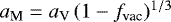 . Therefore, the material heat capacity is assumed to be unchanged.
The effective refractive index meff of the porous grain, from which we can calculate the cross-sections of the porous grain, satisfies the equation (Bohren & Huffman 1983):
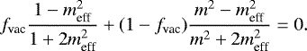 (27)
(27)
Calculations of grain cross-sections are made for porosities of 10, 20 and 30%. To derive the Q coefficients for the porous grains, the calculated cross-sections were normalized by the geometrical cross-section  of the compactsphere of the same mass.
In order to better fit the spectral index of Planck polarization data, we will also present a model where the homogeneous astrosilicate population is replaced by a matrix of astrosilicate (refractive index mm ) with inclusions of a-C (refractive index mi). The resulting refractive index meff is obtained using the Maxwell Garnett rule, better suited than the Bruggeman rule when the volume fraction of a-C inclusions, fi, is small (Bohren & Huffman 1983):
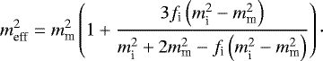 (28)
(28)
5.4 Absorption and scattering coefficients of our dust populations
For each population of astrosilicate and a-C grains, the absorption and scattering coefficients are calculated for grains in perfect spinning alignment with the magnetic field (see Sect. 3), for 70 grain sizes equally spaced in log between a = 3 nm and a = 2 μm, for prolate and oblate grains of various elongations (between 1.5 and 4), and for 800 wavelengths between λ = 0.09 μm and λ = 1 cm.
Figure 3 presents the calculated absorption, extinction, and polarization coeffcients of prolate (ϵ = 1∕3) astrosilicategrains with inclusions of 20% porosity, and different sizes from 0.05 to 2 μm. For the larger grains, the wavelength λ0 below whichcoefficients had to be extrapolated down to the geometric regime are indicated with diamonds (see Sect. 3.3). Figure 4 is the same as Fig. 3, but for prolate (ϵ = 1∕3) a-C grains. The impact of our extrapolation down to the Lyman continuum ought to be modest. First, the heating of big grains by the ISRF is dominated by the optical and NIR radiation, not by the UV radiation. Second, the FUV portion of the polarization curve (λ < 0.15 μm) is ignored in our analysis. Numerical failures described in Sect. 3.3 happen outside of this wavelength range only for grains larger than 0.5 μm, which are absent from our size distributions.
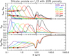 |
Fig. 3 Dust absorption (Qabs), extinction (Qext), and polarization (Qpol) coefficients, as well as the polarization efficiency (Qpol∕Qext), as a function of wavelength, for prolate astrosilicate grains with 20% porosity and an axis ratio ϵ = 1∕3. The radii aV of thevolume-equivalent spheres are indicated. Black diamonds indicate the wavelength λ0 below whichcoefficients had to be extrapolated (see Sect. 3.3). |
5.5 Constraining the shape and composition of the aligned population
Polarization measures provide a direct constraint on the aligned grain population alone. In particular, if silicate grains are aligned, and not carbon grains, the polarization curve in extinction provides some insight into the size distribution of aligned silicate grains (Kim & Martin 1995). In this section, we attempt to adapt the shape and the optical properties of the astrosilicate population to reproduce the RP∕p = P353∕pV polarizationratio. We first test how the grain shape (oblate, prolate) and the axis ratio ϵ affect RP∕p. With the DustEM wrapper, we fit the spectral dependence p(λ) alone for prolate and oblate grains with elongations of 1.5, 2, 3 and 4. The size distribution of astrosilicate grains is a power-law, with adjustable mass per H mdust, slope α and maximal size amax, and a fixed minimal size amin = 3 nm. The alignment parameters, aalig and pstiff, are also adjustable to fit the spectral shape of the curve, while fmax is fixed to 1. At this stage, no a-C nor PAH populations are added, and we voluntarily ignore other dust observational curves (extinction, total emission, polarized emission). The ratio RP∕p is calculated for a mean radiation field intensity (G0 = 1).
Our results are shown in bold in Fig. 5. For oblate grains, we find no effect of the grain elongation on RP∕p: RP∕p ≃ 2.3 MJysr−1 for all elongations up to 4. For prolate grains, we find larger values of RP∕p, increasing from 3 to 5 MJysr−1 when the elongation increases from 1.5 to 4. The reason for this different behaviour between oblate and prolate shapes is illustrated in Fig. 6. This figure shows the polarization cross-sections of prolate and oblate grains of the same size (0.2 μm, typical size of aligned grains), for two values of the elongation, 1.5 and 3. For a given elongation, prolate grains polarize less than oblate grains. This difference is more pronounced in the optical than in the submillimeter (hence the higher values of RP∕p for prolate than for oblate), and tends to increase with the elongation. Concerning the effect of porosity, Fig. 5 also shows that it significantly increases the polarization ratio RP∕p grains by a comparable factor for prolate and oblate grains. This effect is almost independent of the grain axis ratio.
From Fig. 5 we conclude that prolate astrosilicate with elongations between 2 and 4, and porosities between 10 and 30%, are able to reproduce the observed RP∕p polarization ratio, while oblate grains with elongations from 1.5 to 4, even with porosities as high as 30%, are not. Prolate grains with lower elongation and higher porosities would not allow to achieve the maximal polarization in extinction pV ∕AV = 3%.
We also tested the influence of the introduction of a-C inclusions into the astrosilicate matrix. Carbon inclusions tend to flatten the spectral index of the astrosilicate component, and to increase its emissivity, as needed. Our results for 6% of a-C inclusions in volume are presented in Fig. 5 as blue triangles. With a-C inclusions, the same value of RP∕p can be achieved by the astrosilicate population without the need for porosity, and with a smaller elongation of 2.5. We note that our choice for the volume fraction of a-C inclusions is in agreement with the Jones et al. (2013) dust model, where the amorphous silicate component is covered by an aromatic a-C coating that makes up 6% of the total silicate mass.
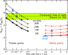 |
Fig. 5 Ratio RP∕p between the polarized emission at 353 GHz, P353, and the polarization degree, pV, measured in extinction in the V band, as a function of the grain axis ratio ϵ, for astrosilicates. Labels indicate the grain porosity. The mean value of RP∕p in translucent lines of sight (Paper I), together with its range of uncertainty, is indicated. Blue triangles correspond to an astrosilicate matrix with a-C inclusions (6% in volume). Blue squares correspond to the Draine & Fraisse (2009) dust models (oblate grains with ϵ = 1.4 and ϵ =1.6). |
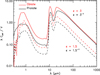 |
Fig. 6 Polarization cross-section per unit volume of the corresponding sphere, λ Cpol ∕V, as a functionof wavelength, for spheroidal grains of equivalent radius aV = 0.2 μm. Results are shown in black for prolate grains, and in red for oblate grains, for an elongation of 3 (solid) and 1.5 (dashed). |
5.6 Dust models
It has been demonstrated that the polarization curve in extinction (pλ) can be fitted with aligned silicate grains alone, or with both aligned silicate and carbon grains (Draine & Fraisse 2009; Siebenmorgen et al. 2014). We present models for both cases:
- 1.
Model A: astrosilicate grains are aligned, a-C grains have a random orientation.
- 2.
Model B: like A, but with the optical properties of Li & Draine (2001) for astrosilicate grains (see Sect. 5.1).
- 3.
Model C: both astrosilicate and a-C grains are aligned, with the same alignment parameters aalig, pstiff and fmax for both populations.
- 4.
Model D: like C, with the homogeneous astrosilicate population replaced by an astrosilicate matrix with 6% of a-C inclusions, in volume.
The question of whether carbon grains are aligned or not is still debated. From the observational point of view, the absence of polarization of the aliphatic 3.4 μm band (Adamson et al. 1999; Chiar et al. 2006) indicates that aliphatic carbon matter (whether as mantles onto silicategrains, or as an independent population) is not or weakly polarizing. However there are no observational constraints in polarization on aromatic carbon grains; the kind that we use here. As demonstrated in Jones et al. (2013), small aromatic carbon mantles would not produce a spectroscopic signature at 3.3 μm because of the small carbon mass involved in the mantle compared to the silicate core. We cannot therefore exclude that aromatic carbon grains could be aligned and polarizing, or that silicate grains could be covered by an aromatic carbonaceous mantle like in the Jones et al. (2013) dust model. To be aligned, carbon grains would need some magnetic properties, at least paramagnetic, to precess around magnetic field lines.
Here weassume, for simplicity, that a-C grains have the same shape and elongation as astrosilicates. As we have seen in Sect. 5.5, prolate astrosilicate grains with an elongation between 2 and 4 are compatible with the observed value for RP∕p, provided that the astrosilicate matrix is made porous. Another constraint on the elongation of grains, both astrosilicate and a-C, is the observed emission per unit extinction. To achieve the high observed value of the total intensity per unit extinction I353 ∕AV = 1.2MJysr−1 found in Paper I, the increased emissivity of our porous and elongated astrosilicate population is not enough: we must also increase the emissivity of the a-C population. The elongation of grains, which is necessary to produce polarization when these grains are aligned, can also provide this emissivity increase. We find that, for models A, B and C, prolate astrosilicate and a-C grains with an elongation of 3 (and an inclusion of 20% porosity for astrosilicates) yield the required emissivity7, while grains with an elongation of 2 and 2.5 are not emissive enough to achieve the observed I353 ∕AV. For model D, an elongation of 2.5 is enough. We further discuss this choice of highly elongated and porous grains in Sect. 7.4.
6 Results
In this section, we compare the best-fit of our four models to the data. We recall that the intensity of the radiation field, G0, is not8 a free parameter: G0 = 1 (see Sect. 5.2). Each model has ten free parameters, including three for dust alignment. Each fit was obtained assuming that none of the four curves should dominate over the others during the fit (see Sect. 4.5). Any other assumption would have lead to different solutions. The  for each curve i, together with the characteristic ratios RV, RP∕p, Rs/V, I353 ∕AV, P353∕I353 and pV ∕τV are given for all models in Table 2. All models reproduce the observational emission-to-extinction ratios within the uncertainties (see Sect. 4).
Reduced χ2 for dust models A, B, C, and D, together with their characteristic ratios.
6.1 Size distributions and elemental abundances
Figure 7 presents the size distribution of PAHs, a-C, and astrosilicate grains for our four models, and compares them to the grain size distribution of the Compiègne et al. (2011) dust model. The maximal size for astrosilicate grains ranges from 0.3 to 0.5 μm depending on the model, with a slope similar to that of Compiègne et al. (2011). The PAH component is larger, as justified in Sect. 5.1. The a-C size distribution is very different from that of Compiègne et al. (2011). It is very steep, with an index close to − 4.5. This is due to the combination of 3 factors: 1) our models do not include any VSG population (Compiègne et al. 2011) to reproduce the IRAS mid-IR emission bands; 2) the 60 to 100 μm color ratio of our SED is higher by a factor ~50% than in Compiègne et al. (2011, see Fig. 1 and Table 1); 3) our a-C population, with its prolate shape (elongation of 3), is more emissive than a-C spheres, and therefore colder.
The resulting parameters for each model are listed in Table 3. The elemental abundances consumed by our models are between 30 and 38 ppm for Si, Mg and Fe. These values are of the order of the recommended solar abundances by Lodders (2003) of 41.7, 40.7 and 34.7, respectively. This is also much less than in the Compiègne et al. (2011) dust model which uses 45 ppm of Si, Mg, and Fe. This is primarily a consequence of the porosityintroduced in the astrosilicate matrix, and of the prolate elongated shape of a-C and astrosilicate grains.
In translucent lines of sight, depletions are observed to increase with the local average density (Jenkins 2009), so the elemental reservoir available for dust is higher in translucent lines of sight than in the diffuse ISM. This is particularly true for carbon (Parvathi et al. 2012). Our models consume between 165 and 188 ppm of carbon, less than the Compiègne et al. (2011) model (200 ppm). Models C and D, where a-C grains are aligned, necessitate less silicium, iron and magnesium, but more carbon, than modelsA and B.
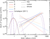 |
Fig. 7 Grain size distribution for each population of our four models: PAH (dot-dashed), a-C (dotted) and astrosilicate (dashed). See Table 3 for the corresponding model parameters. The grain size distribution of the Compiègne et al. (2011) dust model is shown for comparison. |
6.2 Extinction and emission
The extinction curve (Fig. 8) is reasonably well reproduced (χ2 (τ(λ))∕nτ ≪ 1 with 10% error bars), with an extinction-to-reddening ratio RV close to its standard value for the diffuse ISM (RV = 3.1, Fitzpatrick & Massa 2007), except for model C which uses more a-C and less astrosilicate in mass than models A, B and D.
Figure 9 shows the albedo for each model and compares it to observational data and predictions from current models. Ourmodels clearly have too low an albedo, in the optical and in the NIR. This is a problem we could not solve with the particular a-C material used here, the BE sample of Zubko et al. (1996). See Appendix A for a comparison of the extinction properties of the BE sample with other carbonaceous material.
Our models are severely constrained by the dust SED shown in Fig. 10, especially by its 1% error bars in the submillimeter (see Table 1). Model B fails to fit the submillimeter emission: the spectral index of a-C grains (β ~ 1.5) and of the Li & Draine (2001) astrosilicates (β ~ 1.6) are too low to get a good fit. All models fail to reproduce the dust SED at the DIRBE 140 and 240 micron bands. This was already a limitation of the Compiègne et al. (2011) model, that we do not intend to correct here.
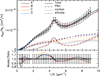 |
Fig. 8 Extinction cross-section per H for our four models as a function of inverse wavelength, with the contribution of each component. Error bars are of 10%, except around the V band where it is 1%. The lower panel represents a normalized version of the upper panel, where each model has been divided by the data value at each frequency of measure to emphasize the difference between models. |
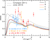 |
Fig. 9 Albedo for our four models as a function of inverse wavelength, compared to existing dust models (Compiègne et al. 2011; Jones et al. 2013). Observational data: red triangles (Lillie & Witt 1976), orange diamonds (Morgan 1980), blue squares(Laureijs et al. 1987). |
6.3 Polarization
The polarization curve in extinction is shown in Fig. 11. Models A and B, where a-C grains are not aligned, do not reproduce well the NIR polarization like models C and D, for which a-C grains are aligned. Kim & Martin (1995) had already demonstrated that, by aligning only astrosilicates, the NIR polarization can only be fitted by adding a population of very large (a ~ 1 μm) grains. Thiscomponent, which is not a simple extension of the power-law to large grain sizes, cannot be accommodated by our parametrization. In Sect. 7.1, we discuss the possible contribution of large (a ~ 1 μm) astrosilicate grains to the NIR polarization curve by adding an exponential tail to our power-law description of the grain size distribution.
The peaking wavelength of the 9.7 μm polarization band is an interesting information to constrain the shape and composition of aligned silicates (Lee & Draine 1985; Hildebrand & Dragovan 1995). We did not intend to fit the profile of this band, but we present their predicted profiles in Fig. 11. We notice that the a-C inclusions in the astrosilicate matrix tend to slightly shift the band to lower wavelengths.
The polarized SED, shown in Fig. 12, is either too steep compared to the data (model A with its spectral index β =2.0 for astrosilicates) or too flat (model B with β = 1.6 for astrosilicates), hence the bad χ2∕n values in Table 2. Aligning a-C grains (Model C) helps to reconcile our model with the low spectral index of the polarized emission observed by Planck, though only partly. Model D, with its composite grains mixing astrosilicate with 6% in volume of a-C, performs the best because, in that particular case, all aligned grains have a low β.
Figure 13 presents the polarization fraction in emission. Model B, with a β =1.6 spectral index for astrosilicate, yields a reasonable profile, but at the expense of a bad fit to the spectral dependence of the total, Iν (λ), and polarized, Pν(λ), intensities (Figs. 10 and 12). Model D is the closest to the data, but still not flat enough. With their aligned a-C grains, models C and D produce higher polarization fractions in the Wien part of the spectrum (e.g., at 100 μm) than model A and B where carbon grains are randomly aligned. This is simply due to the fact that a-C grains and astrosilicate grains with a-C inclusions are warmer than pure astrosilicate grains.
The corresponding grain alignment functions are presented in Fig. 14. The characteristic size for grain alignment (aalig) is close to 0.1 μm in all models, as expected (Kim & Martin 1995; Draine & Fraisse 2009; Voshchinnikov et al. 2016).
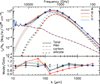 |
Fig. 10 Dust emission SED as a function of wavelength, for our four models, with the contribution of each component. Data points and error bars are from Table 1, with a lower limit of 1% on error bars (see Sect. 4.3). Diamonds indicate for each model the color-corrected value of the modeled SED in each band of Table 1 (approximately + 12% at 353 GHz). |
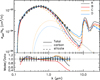 |
Fig. 11 Polarization cross-section per H from the UV to the mid-IR, as a function of wavelength, for our four models. Carbon grains produce negative polarization in the UV (that is, polarization rotated by 90°). |
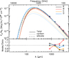 |
Fig. 12 Dust polarized SED as a function of wavelength, for our four models, with the contribution of each component. The derivation of data points with their error bars is detailed in Sect. 4.4. Diamonds indicate for each model the color-corrected value of the modeled SED in each Planck HFI polarized band. |
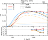 |
Fig. 13 Polarization fraction in emission P∕I as a function of wavelength, for our four models. Data points and error bars are from Planck Collaboration Int. XXII (2015). |
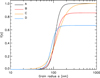 |
Fig. 14 Grain alignment efficiency f(a), as a functionof grain radius a, for our four models. See Eq. (1) for the expression of f and Table 3 for the corresponding alignment parameters. |
7 Discussion
In this section, we discuss to what extent our results constrain the size, shape, composition and alignment efficiency of grains.
7.1 Could large astrosilicate grains also explain the high value of RP∕p = P353∕pV?
We did not explore the possible presence of a population of very large astrosilicate grains (a ~ 1 μm). Such large and cold grains would increase the polarization ratio RP∕p by contributing significantly to the polarized emission at 353 GHz, while producing polarization in the NIR (Kim & Martin 1995) but not so much in the optical.
We model such a population of large astrosilicate grains by an exponential decay attached to the power-law, as per Compiègne et al. (2011), up to aV = 2 μm. This adds three new parameters to the size distribution: ac, at and γ (for a description of those parameters, see Compiègne et al. 2011). Following the same approach as in Sect. 5.5, we use DustEM to fit the p(λ) polarizationcurve with this single aligned population. We obtain a very good fit (χ2 (p(λ))∕np = 0.09) with a size distribution similar to that of Kim & Martin (1995). The polarization ratio is however almost unchanged: RP∕p = 5.9 MJysr−1. We conclude that very large astrosilicate grains (aV ~ 1 μm) do help fitting the NIR polarization curve, but do not contribute significantly to the observed large value of the polarization ratio RP∕p.
7.2 What is the maximal grain alignment efficiency in translucent lines of sight?
The maximal and mean polarization fractions in extinction and in emission are known to decrease with increasing column density (e.g., Whittet et al. 2008; Planck Collaboration Int. XX 2015; Fissel et al. 2016). Two interpretations are usually favoured: 1) the grain alignment efficiency, which depends on the environment, may decrease when entering dense clouds due to the extinction of UV photons by dust grains (Andersson & Potter 2007); 2) the magnetic disorder along the line of sight may induce depolarization, an effect which increases with the column density (Jones et al. 1992; Planck Collaboration Int. XX 2015). Those effects may combine (Jones et al. 2015). We could also mention a third interpretation, supported by observations in unpolarized extinction and emission: 3) the grains composition and shape, and therefore their polarizing efficiencies, could be modified between the diffuse ISM and translucent lines of sight, by accretion and/or coagulation (Jones et al. 2017). This third option, which greatly increases the complexity of the picture in polarization, is further discussed in Sect. 7.4. Here, for simplicity, we restrict our analysis to the first two interpretations.
On translucent lines of sight, the column density is high enough for depolarization to occur, and high enough to limit the efficiency of radiative torques. If this interpretation is complete, the instrinsic dust polarization fraction, defined as the polarization fraction that would be observed without loss of grain alignment nor depolarization along the line of sight (and therefore, impossible to measure in this medium), must be higher than the one we modeled here, of 3% in extinction and 13% in emission. As a consequence, a dust model for translucent lines of sight should also be able to produce a higher polarization fraction than the one observed in that medium, may be up to 20% in emission – the upper limit observed by Planck at low column densities (Planck Collaboration Int. XIX 2015). This condition would exclude models that already necessitate a perfect grain alignment to reproduce the maximal polarization fractions observed in translucent lines of sight, like models A and C, but not the composite model D. In model D, polarization fractions up to P353∕I353 = 20% in emission and pV∕AV = 4.5% in the optical can be achieved9 by increasing fmax from 0.67 up to 1. Such a high polarization fraction in extinction, never observed yet, could only happen at very low column densities (AV ≪ 0.5).
7.3 The dependence of P/I with the wavelength: models versus observations
Figure 15 presents our predictions for the wavelength dependence of P∕I in models A and D, for a radiation field intensity ranging from G0 = 10−1 to G0 = 103. Next to Planck observations, we have added the polarization spectrum recently measured by the BLASTPol balloon experiment in the translucent part (AV ~ 2.5) of the Vela C molecular cloud (Ashton et al. 2017). We note that, due to the combined effect of the variation in grain alignment and magnetic field direction, we can directly compare the spectral dependence of P∕I between models and observations, but not its amplitude. The trend observed by BLASTPol between 250 and 850 μm is compatible with flatness (Ashton et al. 2017). If we normalize BLASTPol and Planck observations at 850 μm, we get a flat, possibly slightly decreasing trend over a decade in wavelength, from 250 μm to 3 mm. With G0 = 1, model D is here again the closest to observations, while model A departs from those data both at short and large wavelengths.
This flat trend does not seem to be limited to translucent lines of sight. In a previous work (Gandilo et al. 2016), the BLASTPol collaboration already observed a flat spectrum between 250 and 850 microns in the high-density regions (NH ≃ 2 × 1022 cm−2, corresponding to AV = 5–10) of the same cloud, heated by the interstellar radiation field (G0 = 1). At even higher column densities, using airborne observations of dust polarized emission in dense regions (among them M17 and M41), Hildebrand et al. (1995) found a maximal polarization fraction at 100 μm of 9% (for the 99 percentile) for a range τ100 μm = 0.02–0.2 of the dust optical depth (or equivalently a range 5–50 in AV). A polarization fraction of 9% is obtained with a radiation field G0 ~ 10 for model D, and with G0 ~ 100 for model A, which is not unrealistic as those observations were focused on bright regions. This peak of P∕I at 9% at 100 μm is also not so far from what is observed at 353 GHz (850 μm) at the same column densities (Planck Collaboration Int. XIX 2015), and does not therefore exclude the possibility of a flatness of the P∕I spectrum from the far-infrared to the millimeter.
In the frame of the astrosilicate-graphite model of Draine & Hensley (2013), the slightly decreasing trend of P∕I with the wavelength has been interpreted as an indication of magnetic dipole emission from iron nano-domains embedded in the silicate matrix. In our models, the polarization fraction in emission P∕I decreases with the wavelength because the astrosilicate population has a much steeper spectral index (β = 2) than the a-C population (β ~ 1.5), that is not compensated by the lower astrosilicate temperature.
More generally, a dust model with a single (or dominating) homogeneous dust population at thermal equilibrium will have a flat P∕I spectrum. In a dust model with two populations of large grains, the decrease of P∕I with λ in the submillimeter may indicate that the population with the highest spectral index is more polarizing (that is, better aligned or intrinsically more polarizing) than the one with the lowest spectral index, akin to the case in all our models. A flat spectrum would indicate that both populations have the same flat spectrum (that is, the same constant P∕I) and different spectral indices, or different flat spectra (that is, different constant P∕I) but the same spectral index. After Ashton et al. (2017), our modeling also confirms that the flatness of the P∕I spectrum in the far-infrared probably indicates that the equilibrium temperature of the aligned population does not differ too much from the equilibrium temperature of the unaligned population, unlike models where only silicates are aligned.
All these observations in translucent lines of sight and dense clouds go against the natural predictions of most dust models, which were designed for the diffuse ISM and based upon two separate dust populations of large grains with distinct optical properties and alignment efficiencies, like carbon and silicate grains. In the following section, we discuss some hints on the composition of dust grains in translucent lines of sight, and how they will need to be related to the evolution of dust properties from the diffuse to the dense ISM.
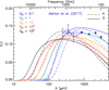 |
Fig. 15 Polarization fraction P∕I in emission for models D (solid) and A (dot-dashed), for various ISRF intensities G0. The spectral shape of the radiation was not changed, just the scaling factor G0, as indicated.Data points combine Planck (λ ≥ 850 μm, Planck Collaboration Int. XXII 2015) and BLASTPol (λ ≤ 850 μm, Ashton et al. 2017) observations, normalized at 850 μm. We cut our spectrum at 5 cm because of the rising contribution to Iν(λ) of the thermal emission of PAH and other components not modeled here (synchrotron emission, anomalous microwave emission, see Planck Collaboration Int. XXII 2015). |
7.4 Can we constrain the shape and composition of aligned grains?
The shape of interstellar grains is constrained by the spectral dependence of the 9.7 μm polarization band (Lee & Draine 1985). Hildebrand & Dragovan (1995) calculated the profile of this band for oblate and prolate astrosilicates and concluded that grains are oblate with an axis ratio ϵ < 3, confirming Lee & Draine (1985) results, in clear contradiction with our models. However, our results do not demonstrate that grains are necessarily porous, prolate, and highly elongated. We did not intend in this paper to determine the shape of interstellar grains, but simply to adapt it to our goal: update the Compiègne et al. (2011) dust model to reproduce dust polarized and unpolarized extinction and emission properties on translucent lines of sight, characterized by increased emissivities. This revision of dust opacity is supported by recent laboratory works. Demyk et al. (2017) measured the opacity of amorphous silicate from the NIR to the submillimeter, and found it much higher (with a mean factor close to 5) than that of astrosilicates. With such highly emissive material, grains of oblate shape will also be able to reproduce the value of the polarization ratios of Paper I.
Our results also provide new insight into the composition of aligned grains. Models with aligned a-C grains (models C and D) have the same number of parameters as models A and B with only astrosilicate grains aligned, and perform better in polarization, both in the NIR and in the submillimeter. This is probably indicating that a-C grains may be aligned or that astrosilicate grains may be contaminated by a-C material (in the form of coating or composite aggregates), at least on our translucent lines of sight (Jones et al. 2013; Köhler et al. 2015). Model D also gives a possible hint in the same direction: models where aligned grains are composite do not need to invoke perfect spinning alignment (fmax = 0.67, see Fig. 14), neither very elongated shapes (elongation 2.5), nor porosity to explain observations.
A physically realistic dust model for polarization should be built on highly emissive, weakly elongated, possibly imperfectly aligned, grains. This approach mixing physically motivated grain shape and composition with optical properties from laboratory data will be pursued in a future work on dust polarization based on the THEMIS approach. The philosophy of the THEMIS framework (Jones et al. 2017) is not to fit new observations, but to provide a consistent physical framework and a set of laboratory data to relate the observed variations of the dust optical properties to the physical processes affecting interstellar grains during their life-cycle through the various phases of the ISM. The THEMIS framework successfully explains the variations of dust emissivity and spectral index from the diffuse to the dense ISM through carbon accretion onto the surface of grains and grain-grain coagulation processes (Köhler et al. 2015; Ysard et al. 2015). It also proposes interesting alternatives to grain growth to explain the phenomenon of coreshine (Jones et al. 2016; Ysard et al. 2016). Calculating the predictions of the THEMIS model in polarization is not a straightfoward task. First, the calculation of the optical properties of THEMIS core-mantle and aggregate grains takes a few months with DDSCAT (Köhler et al. 2015), and even longer when one needs to repeat this work for different grain shapes, a key ingredient for polarization. Second, the evolution of the shape and composition of dust grains should be determined in relation to the physical evolutionary processes affecting dust grains through the ISM, particularly from the diffuse to the dense phase, consistently with polarization observations. This is a work in progress that will be published elsewhere.
8 Summary
DustEM, a modeling tool for dust extinction and emission (Compiègne et al. 2011), was amended to model dust polarization in extinction and in emission. The modeling of grain alignment in DustEM is parametric: the fraction of aligned grains is a function of the grain size through three parameters. Grains cross-sections were calculated for spheroids of prolate and oblate shape, in perfect spinning alignment when they are aligned, and in random alignment when they are not aligned.
We gathered a consistent set of observational data characterizing the spectral dependence of the mean dust extinction, maximal polarization in extinction, mean SED, and maximal polarized SED on translucent lines of sight (AV = 0.5–2.5). Polarized (resp. total) emission curves were normalized per unit polarized (resp. total) extinction in the optical using the submillimeter-to-optical ratios measured in Paper I: P353∕pV = [5.4 ± 0.5]MJysr−1 (resp. I353 ∕AV = [1.2 ± 0.1]MJysr−1). Combining the Planck radiance map (Planck Collaboration XLVIII 2016) and the Pan-STARRS reddening map (Green et al. 2015), we estimated the radiation field intensity in our sample, and found it compatible with the insterstellar standard radiation field. We therefore assumed G0 = 1 in our modeling.
Our models, derived from the Compiègne et al. (2011) dust model, use PAHs, amorphous carbon (BE, Zubko et al. 1996) and astrosilicates (Weingartner & Draine 2001). In the particular case where only astrosilicates are aligned, we demonstrated that the modeled polarization ratio P353∕pV increases with the grain elongation in the case of prolate grains, but remains constant at P353∕pV ≃ 2.3MJysr−1 in the case of oblate grains. The inclusion of porosity in the silicate matrix increases the P353∕pV ratio in a similar manner for prolate and oblate grains, independently of the grain elongation. We found that porous prolate astrosilicate grains, of elongation a∕b between 2 (with a porosity of 30%) and 4 (with a porosity of 10%), could reproduce the high polarization ratio P353∕pV from Paper I, while oblate grains could not. This result applies to all dust models using aligned astrosilicates, independently of the particular material chosen for the other dust populations. Conclusions for other aligned materials may differ in grain shape, elongation, and porosity. We also showed that the presence of a population of very large (a ≥ 1 μm) astrosilicate grains only marginally affects this polarization ratio, while the alignment of a-C grains makes it decrease slightly.
The observed submillimeter-to-optical ratios P353∕pV and I353∕AV can be both reproduced if the grain shape of a-C and astrosilicate is prolate with an elongation a∕b = 3, and astrosilicates are made porous with 20% of porosity. We presented four models compatible with our data set and with cosmic abundance constraints, with a-C grains aligned or not. The spectral dependencies of the extinction curve, of the polarization curve in extinction, and of the total SED, are well reproduced. All models however generally suffer from an overly low albedo in the optical. The polarized SED is not well reproduced when only astrosilicates are aligned. Models perform slightly better when a-C grains (with their spectral index β ~ 1.5) are also aligned. A composite model where the astrosilicate component is mixed with a small fraction of a-C inclusions (6% in volume) performs even better, while necessitating less elongated (a∕b = 2.5), and less efficiently aligned grains. These new insights into the properties of dust support the scenario of a dominant dust component of carbon-coated silicates as proposed by Jones et al. (2013).
The value and wavelength dependencies of P∕I in our models are globally consistent with far-infrared and submillimeter observations in translucent and dense regions (Hildebrand et al. 1995; Gandilo et al. 2016; Ashton et al. 2017), with a better agreement for our composite model with a-C grains aligned. Because of the lower spectral index of the amorphous carbon population (β ~ 1.5), models reproduce the decrease of the polarization fraction in emission P∕I with the wavelength, without the need for the magnetic dipole emission of metallic domains in the silicate matrix proposed by Draine & Hensley (2013).
The DustEM code, documentation, and input files for our models are available online10. With their simple power-law size distributions, and reduced number of free parameters, our models can be used to analyze multiwavelength polarized and unpolarized data, and study the influence of relevant parameters (Fanciullo et al. 2017).
Acknowledgements
The research leading to these results has received funding from the European Research Council under the European Union’s Seventh Framework Programme (FP7/2007-2013)/ERC grant agreement No. 267934. V. Guillet thanks the anonymous referee for helpful remarks, and N. Voshchinnikov, R. Siebenmorgen, B. Hensley, P. G. Martin and G. Green for useful discussions. This research has made use of NASA’s Astrophysics Data System.
Appendix A: Inconsistency in the use of the BE sample for very small grains
The absorption coefficient of very small carbon grains must present an increase in the UV characteristic of the carbon σ to σ* transition at 13 eV (Jones 2012). This is not the case for the BE sample from Zubko et al. (1996).
Figure A.1 compares the extinction curves for four different types of carbon grains: the BE and ACH2 samples from Zubko et al. (1996), graphite (Draine & Lee 1984) and the amorphous carbon a-C(:H) from Jones et al. (2013). Extinction curves were calculated for a 0.1% of gas mass in dust, and a power-law distribution from 3 and 100 nm with an index α =−4.5 similar to the ones used in the present article for carbon grains. The extinction curves differ one from another: ACH2 and BE samples absorb more than graphite and a-C(:H) in the optical; only graphite presents the π to π* transition at 4.6 μm−1. Still, all samples except BE present an increase in the UV.
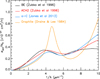 |
Fig. A.1 Extinction cross-section per H as a function of inverse wavelength, for 0.1% of the gas mass in the form of carbon, distributed in a power-law from 3 to 100 nm with an index α = −4.5. Four opticalproperties for carbon are compared: BE and ACH2 (Zubko et al. 1996), a-C(:H) (Jones et al. 2013) and graphite (Draine & Lee 1984). |
Becauseof this inconsistency, the BE sample is probably not the best carbon sample to be used for small carbon grains. This is however of secondary importance in the present article dedicated to the polarized and unpolarized emission of dust grains dominated by large grains. Work is in progress to amend the Jones et al. (2013) dust model for polarization, which will not suffer from this inconsistency.
Appendix B: Cross-sections for perfect spinning alignment with an inclined magnetic field
Let us now consider the general case where the magnetic field is inclined by an angle γ with respect to the plane of the sky, and grains are still in perfect spinning alignment. The cross-section for oblate grains are simply those corresponding to an inclination angle ψ = π∕2 − γ. For prolate grains, we must define the geometry of the problem (Fig. B.1). In the laboratory frame ( ),
),  is directed toward the observer and B lies in the
  plane making an angle γ with
  . The grain is spinning around B. We note α the spin angle between the symmetry axis of the grain and the
  axis. Starting with
  parallel to the
  axis, the orientation of the symmetry axis
  of the grain with respect to the observer can be obtained with two successive Euler transformations:
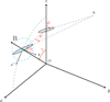 |
Fig. B.1 Geometry of the problem for a prolate grain (here in cyan) spinning around B in perfect alignment. The axis |


- 1.
spinning:
 is rotated by an angle α
around
is rotated by an angle α
around  ;
; - 2.
inclination:
 is rotated by the angle γ
around
is rotated by the angle γ
around  to bring the grain spin axis parallel to B.
After these two rotations, the coordinates of  are ax = −sinα cosγ, ay = cosα, and az = sinα sinγ. The projection of
  onto the plane of the sky makes an angle ϕ with
  :
:
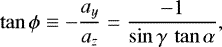 (B.1)
(B.1)
where we follow the IAU sign convention. The grain symmetry axis  makes an angle ψ with the line of sight:
 (B.2)
(B.2)
Integrating over α on the spinning dynamics of the grain, we find the time-averaged cross-sections (Hong & Greenberg 1980):

References
- Adamson, A. J., Whittet, D. C. B., Chrysostomou, A., et al. 1999, ApJ, 512, 224 [NASA ADS] [CrossRef] [Google Scholar]
- Andersson, B.-G., & Potter, S. B. 2007, ApJ, 665, 369 [NASA ADS] [CrossRef] [Google Scholar]
- Andersson, B.-G., Lazarian, A., & Vaillancourt, J. E. 2015, ARA&A, 53, 501 [NASA ADS] [CrossRef] [Google Scholar]
- Ashton, P. C., Ade, P. A. R., Angilè, F. E., et al. 2017, ApJ, submitted [arXiv:1707.02936] [Google Scholar]
- BICEP2/Keck and Planck Collaborations, Ade, P. A. R., Aghanim, N et al. 2015, Phys. Rev. Lett., 114, 101301 [NASA ADS] [CrossRef] [PubMed] [Google Scholar]
- Binggeli, B. 1980, A&A, 82, 289 [NASA ADS] [Google Scholar]
- Bohlin, R. C., Savage, B. D., & Drake, J. F. 1978, ApJ, 224, 132 [NASA ADS] [CrossRef] [Google Scholar]
- Bohren, C. F., & Huffman, D. R. 1983, Absorption and scattering of light by small particles (New York: Wiley) [Google Scholar]
- Boulanger, F., Abergel, A., Bernard, J. P., et al. 1996, A&A, 312, 256 [NASA ADS] [Google Scholar]
- Chandrasekhar, S., & Fermi, E. 1953, ApJ, 118, 113 [NASA ADS] [CrossRef] [Google Scholar]
- Chiar, J. E., Adamson, A. J., Whittet, D. C. B., et al. 2006, ApJ, 651, 268 [CrossRef] [Google Scholar]
- Clayton, G. C., Anderson, C. M., Magalhaes, A. M., et al. 1992, ApJ, 385, L53 [NASA ADS] [CrossRef] [Google Scholar]
- Compiègne, M., Verstraete, L., Jones, A., et al. 2011, A&A, 525, A103 [NASA ADS] [CrossRef] [EDP Sciences] [Google Scholar]
- Dalcanton, J. J., Fouesneau, M., Hogg, D. W., et al. 2015, ApJ, 814, 3 [NASA ADS] [CrossRef] [Google Scholar]
- Das, H. K., Voshchinnikov, N. V., & Il’in, V. B. 2010, MNRAS, 404, 265 [NASA ADS] [Google Scholar]
- Davis, L., & Greenstein, J. L. 1951, AJ, 114, 206 [NASA ADS] [CrossRef] [Google Scholar]
- Demyk, K., Meny, C., Lu, X.-H., et al. 2017, A&A, 600, A123 [NASA ADS] [CrossRef] [EDP Sciences] [Google Scholar]
- Draine, B. T.,& Allaf-Akbari, K. 2006, ApJ, 652, 1318 [NASA ADS] [CrossRef] [Google Scholar]
- Draine, B. T.,& Fraisse, A. A. 2009, ApJ, 696, 1 [NASA ADS] [CrossRef] [Google Scholar]
- Draine, B. T.,& Hensley, B. 2013, ApJ, 765, 159 [NASA ADS] [CrossRef] [Google Scholar]
- Draine, B. T.,& Lee, H. M. 1984, ApJ, 285, 89 [Google Scholar]
- Draine, B. T.,& Li, A. 2007, ApJ, 657, 810 [NASA ADS] [CrossRef] [Google Scholar]
- Draine, B. T.,& Weingartner, J. C. 1996, ApJ, 470, 551 [NASA ADS] [CrossRef] [Google Scholar]
- Draine, B. T.,& Weingartner, J. C. 1997, ApJ, 480, 633 [NASA ADS] [CrossRef] [Google Scholar]
- Fanciullo, L., Guillet, V., Aniano, G., et al. 2015, A&A, 580, A136 [NASA ADS] [CrossRef] [EDP Sciences] [Google Scholar]
- Fanciullo, L., Guillet, V., Boulanger, F., & Jones, A. P. 2017, A&A, 602, A7 [NASA ADS] [CrossRef] [EDP Sciences] [Google Scholar]
- Fissel, L. M., Ade, P. A. R., Angilè, F. E., et al. 2016, ApJ, 824, 134 [NASA ADS] [CrossRef] [Google Scholar]
- Fitzpatrick, E. L. 1999, PASP, 111, 63 [NASA ADS] [CrossRef] [Google Scholar]
- Fitzpatrick, E. L., & Massa, D. 2007, ApJ, 663, 320 [NASA ADS] [CrossRef] [EDP Sciences] [Google Scholar]
- Gandilo, N. N., Ade, P. A. R., Angilè, F. E., et al. 2016, ApJ, 824, 84 [Google Scholar]
- Gorski, K. M., Hivon, E., Banday, A. J., et al. 2005, ApJ, 622, 759 [NASA ADS] [CrossRef] [Google Scholar]
- Green, G. M., Schlafly, E. F., Finkbeiner, D. P., et al. 2015, ApJ, 810, 25 endrefcommentnewpage [NASA ADS] [CrossRef] [Google Scholar]
- Hauser, M. G., Arendt, R. G., Kelsall, T., et al. 1998, ApJ, 508, 25 [NASA ADS] [CrossRef] [Google Scholar]
- Heiles, C. 2000, AJ, 119, 923 [NASA ADS] [CrossRef] [Google Scholar]
- Hildebrand, R. H. 1983, QJRAS, 24, 267 [NASA ADS] [Google Scholar]
- Hildebrand, R. H., & Dragovan, M. 1995, ApJ, 450, 663 [NASA ADS] [CrossRef] [Google Scholar]
- Hildebrand, R. H., Dotson, J. L., Dowell, C. D., et al. 1995, PASP, 73, 97 [Google Scholar]
- Hoang, T., & Lazarian, A. 2016, ApJ, 831, 159 [NASA ADS] [CrossRef] [Google Scholar]
- Hoang, T., Lazarian, A., & Martin, P. G. 2013, ApJ, 779, 152 [NASA ADS] [CrossRef] [Google Scholar]
- Hong, S. S., & Greenberg, J. M. 1980, A&A, 88, 194 [NASA ADS] [Google Scholar]
- Jenkins, E. B. 2009, ApJ, 700, 1299 [NASA ADS] [CrossRef] [Google Scholar]
- Jones, A. P. 1988, MNRAS, 234, 209 [NASA ADS] [Google Scholar]
- Jones, A. P. 2012, A&A, 540, A2 [NASA ADS] [CrossRef] [EDP Sciences] [Google Scholar]
- Jones, T. J., Klebe, D., & Dickey, J. M. 1992, ApJ, 389, 602 [NASA ADS] [CrossRef] [Google Scholar]
- Jones, A. P., Fanciullo, L., Köhler, M., et al. 2013, A&A, 558, A62 [NASA ADS] [CrossRef] [EDP Sciences] [Google Scholar]
- Jones, T. J., Bagley, M., Krejny, M., Andersson, B.-G., & Bastien, P. 2015, AJ, 149, 31 [NASA ADS] [CrossRef] [Google Scholar]
- Jones, A. P., Köhler, M., Ysard, N., et al. 2016, A&A, 588, A43 [NASA ADS] [CrossRef] [EDP Sciences] [Google Scholar]
- Jones, A. P., Köhler, M., Ysard, N., Bocchio, M., & Verstraete, L. 2017, A&A, 602, A46 [NASA ADS] [CrossRef] [EDP Sciences] [Google Scholar]
- Kim, S.-H., & Martin, P. G. 1995, ApJ, 444, 293 [NASA ADS] [CrossRef] [Google Scholar]
- Köhler, M., Ysard, N., & Jones, A. P. 2015, A&A, 579, A15 [NASA ADS] [CrossRef] [EDP Sciences] [Google Scholar]
- Laureijs, R. J., Mattila, K., & Schnur, G. 1987, A&A, 184, 269 [NASA ADS] [Google Scholar]
- Lazarian, A., & Hoang, T. 2007, MNRAS, 378, 910 [Google Scholar]
- Lee, H. M., & Draine, B. T. 1985, ApJ, 290, 211 [NASA ADS] [CrossRef] [Google Scholar]
- Li, A., & Draine, B. T. 2001, ApJ, 554, 778 (LD01) [Google Scholar]
- Lillie, C. F., & Witt, A. N. 1976, AJ, 208, 64 [NASA ADS] [CrossRef] [Google Scholar]
- Lodders, K. 2003, ApJ, 591, 1220 [NASA ADS] [CrossRef] [Google Scholar]
- Markwardt, C. B. 2009, Astronomical Data Analysis Software and Systems XVIII, ASP Conf. Ser., 411, 251 [Google Scholar]
- Martin, P. G. 2007, EAS Pub. Ser., 23, 165 [Google Scholar]
- Martin, P. G., Adamson, A. J., Whittet, D. C. B., et al. 1992, ApJ, 392, 691 [NASA ADS] [CrossRef] [Google Scholar]
- Martin, P. G., Roy, A., Bontemps, S., et al. 2012, ApJ, 751, 28 [NASA ADS] [CrossRef] [Google Scholar]
- Mathis, J. S. 1990, ARA&A, 28, 37 [NASA ADS] [CrossRef] [Google Scholar]
- Min, M., Hovenier, J. W., & de Koter A. 2003, A&A, 404, 35 [NASA ADS] [CrossRef] [EDP Sciences] [Google Scholar]
- Mishchenko, M. I. 2000, Appl. Opt., 39, 1026 [NASA ADS] [CrossRef] [Google Scholar]
- Mishchenko, M. I., Hovenier, J. W., & Travis, L. D. 2000, Light scattering by nonspherical particles: theory, measurements, and applications (San Diego: Academic Press) [Google Scholar]
- Miville-Deschênes, M.-A., & Lagache, G. 2005, ApJS, 157, 302 [NASA ADS] [CrossRef] [Google Scholar]
- Morgan, D. H. 1980, MNRAS, 190, 825 [NASA ADS] [Google Scholar]
- Parvathi, V. S., Sofia, U. J., Murthy, J., & Babu, B. R. S. 2012, ApJ, 760, 36 [NASA ADS] [CrossRef] [Google Scholar]
- Planck Collaboration XI. 2014, A&A, 571, A11 [NASA ADS] [CrossRef] [EDP Sciences] [Google Scholar]
- Planck Collaboration Int. XVII. 2014, A&A, 566, A55 [NASA ADS] [CrossRef] [EDP Sciences] [Google Scholar]
- Planck Collaboration Int. XIX. 2015, A&A, 576, A104 [NASA ADS] [CrossRef] [EDP Sciences] [Google Scholar]
- Planck Collaboration Int. XX. 2015, A&A, 576, A105 [NASA ADS] [CrossRef] [EDP Sciences] [Google Scholar]
- Planck Collaboration Int. XXI. 2015, A&A, 576, A106 (Paper I) [NASA ADS] [CrossRef] [EDP Sciences] [Google Scholar]
- Planck Collaboration Int. XXII. 2015, A&A, 576, A107 [NASA ADS] [CrossRef] [EDP Sciences] [Google Scholar]
- Planck Collaboration VIII. 2016, A&A, 594, A8 [NASA ADS] [CrossRef] [EDP Sciences] [Google Scholar]
- Planck Collaboration XXIX. 2016, A&A, 586, A132 [NASA ADS] [CrossRef] [EDP Sciences] [Google Scholar]
- Planck Collaboration XLVIII. 2016, A&A, 596, A109 [NASA ADS] [CrossRef] [EDP Sciences] [Google Scholar]
- Planck Collaboration Int. L. 2017, A&A, 599, A51 [NASA ADS] [CrossRef] [EDP Sciences] [Google Scholar]
- Rachford, B. L., Snow, T. P., Destree, J. D., et al. 2009, ApJS, 180, 125 [NASA ADS] [CrossRef] [Google Scholar]
- Reissl, S., Wolf, S., & Brauer, R. 2016, A&A, 593, A87 [NASA ADS] [CrossRef] [EDP Sciences] [Google Scholar]
- Santos, F. P., Ade, P. A. R., Angilè, F. E., et al. 2017, ApJ, 837, 161 [NASA ADS] [CrossRef] [Google Scholar]
- Serkowski, K., Mathewson, D. S., & Ford, V. L. 1975, ApJ, 196, 261 [NASA ADS] [CrossRef] [Google Scholar]
- Siebenmorgen, R., Voshchinnikov, N. V., & Bagnulo, S. 2014, A&A, 561, A82 [NASA ADS] [CrossRef] [EDP Sciences] [Google Scholar]
- Stein, W. 1966, ApJ, 144, 318 [NASA ADS] [CrossRef] [Google Scholar]
- Voshchinnikov, N. V., Il’in, V. B., & Das, H. K. 2016, MNRAS, 462, 2343 [NASA ADS] [CrossRef] [Google Scholar]
- Waterman, P. C. 1971, Phys. Rev. D, 3, 825 [Google Scholar]
- Weingartner, J. C., & Draine, B. T. 2001, ApJ, 548, 296 (WD01) [NASA ADS] [CrossRef] [Google Scholar]
- Whittet, D. C. B., Hough, J. H., Lazarian, A., & Hoang, T. 2008, ApJ, 674, 304 [NASA ADS] [CrossRef] [Google Scholar]
- Wolff, M. J., Clayton, G. C., & Meade, M. R. 1993, ApJ, 403, 722 [NASA ADS] [CrossRef] [Google Scholar]
- Wolff, M. J., Clayton, G. C., Kim, S.-H., Martin, P. G., & Anderson, C. M. 1997, ApJ, 478, 395 [NASA ADS] [CrossRef] [Google Scholar]
- Ysard, N., Juvela, M., Demyk, K., et al. 2012, A&A, 542, A21 [NASA ADS] [CrossRef] [EDP Sciences] [Google Scholar]
- Ysard, N., Abergel, A., Ristorcelli, I., et al. 2013, A&A, 559, A133 [NASA ADS] [CrossRef] [EDP Sciences] [Google Scholar]
- Ysard, N., Köhler, M., Jones, A., et al. 2015, A&A, 577, A110 [NASA ADS] [CrossRef] [EDP Sciences] [Google Scholar]
- Ysard, N., Köhler, M., Jones, A., et al. 2016, A&A, 588, A44 [NASA ADS] [CrossRef] [EDP Sciences] [Google Scholar]
- Zhukovska, S., Dobbs, C., Jenkins, E. B., & Klessen, R. S. 2016, ApJ, 831, 147 [NASA ADS] [CrossRef] [Google Scholar]
- Zubko, V., Mennella, V., Colangeli, L., & Bussoletti, E. 1996, MNRAS, 282, 1321 [NASA ADS] [CrossRef] [Google Scholar]
- Zubko, V., Dwek, E., & Arendt, R. G. 2004, ApJS, 152, 211 [NASA ADS] [CrossRef] [Google Scholar]
The version of DustEM with polarization can be downloaded from http://www.ias.u-psud.fr/DUSTEM
For more information, see http://healpix.jpl.nasa.gov and http://healpix.sourceforge.net
For ϵ = 1∕3, this happens when aV∕λ ≃ 3. For ϵ = 1∕4, this happens when aV∕λ ≃ 1.7.
The starlight polarization degree, p, a percentage, is not to be confused with the polarization fraction of dust extinction, also often noted as p (here denoted as p∕τ).
Like thermal emission in the far-infrared and submillimeter, extinction in the V band is mainly sensitive to the amount of large (a ~ 0.1 μm) dust grains on the line of sight.
The submillimeter absorption cross-section of a-C grains of prolate shape and elongation increase by a factor 3.4 with respect to spheres. WD01 prolate astrosilicate grains of elongation 3 with 20% porosity, by a factor 2.4. This is in contrast with the optical: their extinction cross-sections are almost unchanged for a-C grains, and decrease only by 20% for astrosilicates.
Fixing G0, we give ourselves less flexibility in fitting the shape of the total and polarized SEDs. This is done on purpose, to directly test the optical properties of our dust populations against emission data.
This linearity between the polarization in extinction and in emission is a consequence of our parametric modeling of dust alignment (see Sect. 2.1). The limits of this hypothesis will be studied in a dedicated paper.
All Tables
Reduced χ2 for dust models A, B, C, and D, together with their characteristic ratios.
All Figures
|
Fig. 1 (Black) New reference SED for translucent lines of sight (5 < I857 < 20 MJysr−1), converted into a SED per AV assuming I353∕AV = 1.2 MJysr−1. Errors bars include statistical and gain uncertainties, but not the systematic uncertainty of 0.1 MJysr−1 on I353 ∕AV from Paper I (see Sect. 4.3). (Red) SED measured in the high Galactic latitude ISM by Planck Collaboration XXIX (2016). (Blue) Dust SED from the Compiègne et al. (2011) model. |
| In the text | |
|
Fig. 2 Planck dust temperature, T, as a functionof our estimate for the radiation field intensity, |
| In the text | |
|
Fig. 3 Dust absorption (Qabs), extinction (Qext), and polarization (Qpol) coefficients, as well as the polarization efficiency (Qpol∕Qext), as a function of wavelength, for prolate astrosilicate grains with 20% porosity and an axis ratio ϵ = 1∕3. The radii aV of thevolume-equivalent spheres are indicated. Black diamonds indicate the wavelength λ0 below whichcoefficients had to be extrapolated (see Sect. 3.3). |
| In the text | |
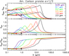 |
Fig. 4 Same as Fig. 3, for prolate (ϵ = 1∕3) a-C grains. |
| In the text | |
|
Fig. 5 Ratio RP∕p between the polarized emission at 353 GHz, P353, and the polarization degree, pV, measured in extinction in the V band, as a function of the grain axis ratio ϵ, for astrosilicates. Labels indicate the grain porosity. The mean value of RP∕p in translucent lines of sight (Paper I), together with its range of uncertainty, is indicated. Blue triangles correspond to an astrosilicate matrix with a-C inclusions (6% in volume). Blue squares correspond to the Draine & Fraisse (2009) dust models (oblate grains with ϵ = 1.4 and ϵ =1.6). |
| In the text | |
|
Fig. 6 Polarization cross-section per unit volume of the corresponding sphere, λ Cpol ∕V, as a functionof wavelength, for spheroidal grains of equivalent radius aV = 0.2 μm. Results are shown in black for prolate grains, and in red for oblate grains, for an elongation of 3 (solid) and 1.5 (dashed). |
| In the text | |
|
Fig. 7 Grain size distribution for each population of our four models: PAH (dot-dashed), a-C (dotted) and astrosilicate (dashed). See Table 3 for the corresponding model parameters. The grain size distribution of the Compiègne et al. (2011) dust model is shown for comparison. |
| In the text | |
|
Fig. 8 Extinction cross-section per H for our four models as a function of inverse wavelength, with the contribution of each component. Error bars are of 10%, except around the V band where it is 1%. The lower panel represents a normalized version of the upper panel, where each model has been divided by the data value at each frequency of measure to emphasize the difference between models. |
| In the text | |
|
Fig. 9 Albedo for our four models as a function of inverse wavelength, compared to existing dust models (Compiègne et al. 2011; Jones et al. 2013). Observational data: red triangles (Lillie & Witt 1976), orange diamonds (Morgan 1980), blue squares(Laureijs et al. 1987). |
| In the text | |
|
Fig. 10 Dust emission SED as a function of wavelength, for our four models, with the contribution of each component. Data points and error bars are from Table 1, with a lower limit of 1% on error bars (see Sect. 4.3). Diamonds indicate for each model the color-corrected value of the modeled SED in each band of Table 1 (approximately + 12% at 353 GHz). |
| In the text | |
|
Fig. 11 Polarization cross-section per H from the UV to the mid-IR, as a function of wavelength, for our four models. Carbon grains produce negative polarization in the UV (that is, polarization rotated by 90°). |
| In the text | |
|
Fig. 12 Dust polarized SED as a function of wavelength, for our four models, with the contribution of each component. The derivation of data points with their error bars is detailed in Sect. 4.4. Diamonds indicate for each model the color-corrected value of the modeled SED in each Planck HFI polarized band. |
| In the text | |
|
Fig. 13 Polarization fraction in emission P∕I as a function of wavelength, for our four models. Data points and error bars are from Planck Collaboration Int. XXII (2015). |
| In the text | |
|
Fig. 14 Grain alignment efficiency f(a), as a functionof grain radius a, for our four models. See Eq. (1) for the expression of f and Table 3 for the corresponding alignment parameters. |
| In the text | |
|
Fig. 15 Polarization fraction P∕I in emission for models D (solid) and A (dot-dashed), for various ISRF intensities G0. The spectral shape of the radiation was not changed, just the scaling factor G0, as indicated.Data points combine Planck (λ ≥ 850 μm, Planck Collaboration Int. XXII 2015) and BLASTPol (λ ≤ 850 μm, Ashton et al. 2017) observations, normalized at 850 μm. We cut our spectrum at 5 cm because of the rising contribution to Iν(λ) of the thermal emission of PAH and other components not modeled here (synchrotron emission, anomalous microwave emission, see Planck Collaboration Int. XXII 2015). |
| In the text | |
|
Fig. A.1 Extinction cross-section per H as a function of inverse wavelength, for 0.1% of the gas mass in the form of carbon, distributed in a power-law from 3 to 100 nm with an index α = −4.5. Four opticalproperties for carbon are compared: BE and ACH2 (Zubko et al. 1996), a-C(:H) (Jones et al. 2013) and graphite (Draine & Lee 1984). |
| In the text | |
|
Fig. B.1 Geometry of the problem for a prolate grain (here in cyan) spinning around B in perfect alignment. The axis |
| In the text | |
Current usage metrics show cumulative count of Article Views (full-text article views including HTML views, PDF and ePub downloads, according to the available data) and Abstracts Views on Vision4Press platform.
Data correspond to usage on the plateform after 2015. The current usage metrics is available 48-96 hours after online publication and is updated daily on week days.
Initial download of the metrics may take a while.