| Issue |
A&A
Volume 606, October 2017
|
|
|---|---|---|
| Article Number | A36 | |
| Number of page(s) | 13 | |
| Section | Extragalactic astronomy | |
| DOI | https://doi.org/10.1051/0004-6361/201629519 | |
| Published online | 05 October 2017 | |
Light breeze in the local Universe
1 Excellence Cluster Universe, Boltzmannstr. 2, 85748 Garching, Germany
e-mail: This email address is being protected from spambots. You need JavaScript enabled to view it.
2 Dipartimento di Fisica e Astronomia, Universitá degli Studi di Bologna, V. le Berti Pichat, 6/2 – 40127 Bologna, Italy
3 INAF-Osservatorio Astronomico di Bologna, via Ranzani 1, 40127 Bologna, Italy
4 European Southern Observatory, Karl-Schwarzschild-str. 2, 85748 Garching, Germany
Received: 11 August 2016
Accepted: 22 March 2017
Abstract
We analyze a complete spectroscopic sample of galaxies (~600 000) drawn from Sloan Digital Sky Survey (SDSS, DR7) to look for evidence of galactic winds in the local Universe. We focus on the shape of the [OIII]λ5007 emission line as a tracer of ionizing gas outflows. We stack our spectra in a fine grid of star formation rate (SFR) and stellar mass to analyze the dependence of winds on the position of galaxies in the SFR versus mass diagram. We do not find any significant evidence of broad and shifted [OIII]λ5007 emission line which we interpret as no evidence of outflowing ionized gas in the global population. We have also classified these galaxies as star-forming or AGN-dominated according to their position in the standard BPT diagram. We show how the average [OIII]λ5007 profile changes as a function of the nature of the dominant ionizing source. We find that in the star-forming dominated source the oxygen line is symmetric and governed by the gravitational potential well. The AGN or composite AGN\star-formation activity objects, in contrast, display a prominent and asymmetric profile that can be well described by a broad Gaussian component that is blue-shifted from a narrow symmetric core. In particular, we find that the blue wings of the average [OIII]λ5007 profiles are increasingly prominent in the LINERs and Seyfert galaxies. We conclude that, through the identification of strong bulk motion as traced by the warm ionized gas, in the low-redshift Universe, “pure” star-formation activity does not seem capable of driving ionized-gas outflows, while, the presence of optically selected AGN seems to play a primary role. We discuss the implications of these results for the role of the quenching mechanism in the present-day Universe.
Key words: Galaxy: evolution / intergalactic medium / galaxies: star formation / quasars: emission lines / ISM: jets and outflows / ISM: kinematics and dynamics
© ESO, 2017
1. Introduction
The most striking feature of the history of our Universe is a drastic decrease in the star-formation activity of the galaxy population by almost an order of magnitude over the last 10 Gyr, after a phase of high and rather constant activity (e.g., Lilly et al. 1996; Madau et al. 1998; Madau & Dickinson 2014, for a comprehensive review). Which process or which combination of processes, leading to the so called “quenching” of the star formation activity, causes such a decrease is still a matter of intensive debate. It is apparent that identifying the quenching process(es) is crucial to establishing a complete view of how galaxies evolve across cosmic time.
According to the most accredited galaxy formation models, from the semi-analytical (SAM) ones to the more recent mass-abundance-matching models, in the central galaxies, the efficiency in converting the gas fraction into stars reaches a maximum at halo mass ~1012M⊙ with only ~20% of their baryons currently locked up in stars (see for example Croton et al. 2006; Guo et al. 2011, based on the Millennium Simulation, and Moster et al. 2010; Behroozi et al. 2010; Yang et al. 2012, among the mass-abundance-matching models). The efficiency drops down steeply towards both sides of this mass threshold (e.g., Madau et al. 1996; Baldry et al. 2008; Conroy & Wechsler 2009; Guo et al. 2010; Moster et al. 2010, 2013; Behroozi et al. 2010, 2013). There is an overall agreement, from the theoretical point of view, that below halo masses of 1012M⊙, the decreasing SF efficiency is likely to be due to gas eating and removal associated with the star-formation activity. Indeed, galactic winds driven by the energy and momentum imprinted by massive stars to the surrounding ISM, are believed to be sufficiently energetic to eject the gas away from the galaxy potential well and quench the star formation (see for instance Chevalier 1977 for energy-driven outflows, Murray et al. 2005 for momentum-driven outflows, and to Hopkins et al. 2014 for effect of multiple stellar feedback in cosmological simulations). Above stellar masses of 1012M⊙, instead, more powerful outflows are required to let the gas escape from the deeper galaxy potential well. The energy and radiation generated by accretion onto the massive black hole (BH), in the most massive galaxies, exceeds the binding energy of the gas by a large factor (see Fabian 2012, for a complete review). Therefore, energetic feedback from active galactic nuclei (AGN) is believed to provide an important and effective mechanism to eject the gas away by powerful winds, stop the growth of the galaxy and stifle accretion onto the BH (Di Matteo et al. 2005; De Lucia et al. 2006; Croton et al. 2006; Hopkins et al. 2006, 2014; Bower et al. 2006; Henriques et al. 2017).
However, although these models are very successful in reproducing a large variety of observational evidence, in particular, the evolution of the stellar mass function (e.g., Henriques et al. 2017), they still lack a clear observational confirmation. Indeed, a lot of effort has been made in the last decade from the observational point of view to observe the presence of such outflows at any mass scale and to study their effect on the evolution of the galaxy star-formation activity to identify a possible relation of cause and effect. Steidel et al. (2010) observe blue-shifted Lyman-α emission in most of the star-forming (SF) galaxy population at redshift ~2 and associate such emission line disturbance to star-formation-induced outflow (see also Erb 2015, for different emission line study). At somewhat lower redshift, but in a large redshift window (0.5 <z< 1.5), Martin et al. (2012) use UV rest-frame absorption features to identify blue-shifted components as indication of outflow and find evidence of outflowing material in massive, highly star-forming galaxies (see also Rubin et al. 2014, for similar studies).
Powerful AGN-driven outflows have recently been observed both at low (e.g., Feruglio et al. 2010; Villar-Martín et al. 2011; Rupke & Veilleux 2011; Rupke & Veilleux 2013; Greene et al. 2012; Mullaney et al. 2013; Rodríguez Zaurín et al. 2013; Cicone et al. 2014) and high redshift (e.g., Maiolino et al. 2012; Tremonti et al. 2007; Brusa et al. 2015; Perna et al. 2015; Cresci et al. 2015). However, it is not clear yet if the AGN feedback, in the form of galactic flows, is a specific property of the bulk of the AGN population or if it concerns only a subclass of these objects (Brusa et al. 2015). In addition, it is unclear if they cause a quenching or an enhancement of the galaxy SF activity (e.g., Cresci et al. 2015).
Furthermore, new observations are revealing the ubiquity of SF-induced outflows in very actively star-forming galaxies at all cosmic epochs (see Veilleux et al. 2005 and Erb 2015, for a comprehensive overview). They are usually associated with energetic starburst phenomena (e.g., Heckman et al. 1990; Pettini et al. 2000; Shapley et al. 2003; Rupke et al. 2002, 2005a,b; Martin 2005, 2006; Hill & Zakamska 2014), while their impact in the normal star-forming galaxies (Chen et al. 2010; Martin et al. 2012; Rubin et al. 2014; Cicone et al. 2016) and their global effect on the baryon cycle is still debated (Steidel et al. 2010).
These studies have traditionally been carried out with relatively small samples of galaxies. The availability of large spectroscopic data sets such as the SDSS (York et al. 2000), allows us to dramatically extend such studies in size. Significant improvement has recently been made in this regard (e.g., Greene & Ho 2005; Chen et al. 2010; Mullaney et al. 2013; Cicone et al. 2016). However, all these resent works have only focused on a particular category of galaxy. For example, the optically-selected AGN in Mullaney et al. (2013) and Greene & Ho (2005) and the star-forming galaxies without AGN contribution in Chen et al. (2010) and Cicone et al. (2016).
The aim of this paper is to explore the global proprieties of galactic winds in the local Universe a) by analyzing their incidence in the galaxy population; b) by identifying the powering mechanism: star formation, AGN or a mixed contribution of the two; and c) by clarifying what impact they might have on the galaxy SF activity. For this purpose we investigate the outflow signatures in a large sample of optical spectra at redshift z< 0.3, drawn from the Sloan Digital Sky Survey (SDSS; Abazajian et al. 2009), by using the ionized gas as traced by the [OIII]λ5007 emission line. The [OIII]λ5007 emission line is one of the strongest features in the rest-frame optical 1D spectrum of both active star-forming and AGN-dominated galaxies. This line is produced through a forbidden transition emitted by low-density and warm gas (T ~ 104 K). Thus, any disturbed kinematic, such as a broadening and asymmetry of the [OIII] line, is only due to the presence of strong bulk motions of ionized interstellar gas (e.g., for local galaxies Heckman et al. 1990; Veilleux et al. 1995; Lehnert & Heckman 1996; Soto et al. 2012; Westmoquette et al. 2012; Mullaney et al. 2013; Rodríguez Zaurín et al. 2013; Bellocchi et al. 2013; Rupke & Veilleux 2013; Liu et al. 2013; Harrison et al. 2014; Zakamska & Greene 2014; Cazzoli et al.2014; Arribas et al. 2014; Cicone et al. 2016, and at high redshift Shapiro et al. 2009; Newman et al. 2012; Harrison et al. 2012; Cano-Díaz et al. 2012; Genzel et al. 2014; Förster Schreiber et al. 2014; Brusa et al. 2015; Perna et al. 2015; Carniani et al. 2015). Also, [OIII]λ5007 emission is expected to lie in spectral regions free from strong stellar atmospheric absorptions. In this respect, it is expected that the [OIII]λ5007 emission line can be used with great success to identify or confirm galactic winds. We explore how the emission line profile changes as a function of key physical parameters: stellar mass, star formation rate (SFR), and primary photoionization processes (SF, AGN). In doing so, we analyze both the presence of a second broader Gaussian component and non-parametric variation of the line-profile.
This work is organized as follows. In Sect. 2, we present our sample selection and physical properties. In Sect. 3, we describe the method used to extract and analyze the [OIII]λ5007 emission line from our stacked spectra. We present and discuss the main results in Sect. 4 and finally we summarize our findings in Sect. 5. Throughout this paper, we assume the following cosmological parameters: H0 = 70 km s-1 Mpc-1, ΩM = 0.3 and ΩΛ = 0.7.
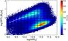 |
Fig. 1 SFR-M⋆ plane for DR7 SDSS galaxies. The black boxes represent the fine grid used for the stacking of the total sample.The white line shows the position of the so-called “main sequence” (MS) of star−forming galaxies. The MS is computed as the mode and the dispersion of the SFR distribution in stellar mass bins following the example of Renzini & Peng (2015). |
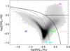 |
Fig. 2 Distribution of the galaxies in our sample in the BPT line-ratio diagram. The solid curve is the theoretical demarcation of Kewley et al. (2001) , that separates star-forming galaxies and composites from AGN. The dashed (Kauffmann et al. 2003a ) and dotted Stasinska et al. (2006) curves indicate the empirical division between composite SF-AGN and AGN-SF and the pure star-forming galaxies, respectively (see text for more details). The horizontal line at log ([OIII]/Hβ) = 0.5 is the demarcation criteria between TYPE 2 (or Seyfert, Sy) and LINERs galaxies showed in Kewley et al. (2006). |
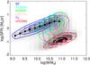 |
Fig. 3 Location of SF, SF−AGN, AGN−SF, LINERs, TYPE 2 (or Sy) and unClass galaxies in the SFR-M⋆ plane. From outside to inside, the contours encompass 25, 50, and 75 per cent of the data points. The black line shows the mode and dispersion of the MS. |
2. Data sample
2.1. SDSS spectra
The galaxy sample analyzed in this paper is drawn from the Sloan Digital Sky Survey, (SDSS, York et al. 2000). In particular, we use the spectroscopic catalog containing ~930 000 spectra belonging to the seventh data release (DR7, Abazajian et al. 2009). We use only objects included in the Main Galaxy Sample (MGS, Strauss et al. 2002) which have Petrosian magnitude r< 17.77 and redshift distribution extending from 0.005 to 0.30, with a median z of 0.10. The spectra cover a wavelength range from 3800 to 9200 Å. They are obtained with 3′′ diameter aperture fibers that, in the adopted cosmology, corresponds to ≈0.31 − 13.36 kpc for the redshift range z = 0.005 − 0.3. The instrumental resolution is R ≡ λ/δλ ~ 1850 − 2200 with a mean dispersion of 69 km s-1. Further details concerning the DR7 spectra can be found online1.
2.2. Star-formation rates and stellar masses
We adopt the star formation – stellar mass plane (hereafter SFR-M⋆) in order to classify galaxies in their fundamental properties. In order to define the position for each galaxy in the SFR-M⋆ plane, we use the SFR and M⋆ measurements taken from the MPA-JHU catalog2. The stellar masses are obtained from a fit to the spectral energy distribution (SED) by using the SDSS broad-band optical photometry (see Kauffmann et al. 2003b for more exhaustive details). The SFR measurements are based on the Brinchmann et al. (2004) approach. They use the Hα emission line luminosity to determine the SFRs for the star-forming galaxies. For all other galaxies, which have emission lines contaminated by AGN activity or unmeasurable emission lines, the SFRs are inferred by D4000-SFR relation (e.g., Kauffmann et al. 2003b). All SFR measurements are corrected for the fiber aperture following the approach proposed by Salim et al. (2007).
We apply a stellar mass cut at log (M/M⊙) ≥ 9.0 to limit the incompleteness in the low-mass regime (see also Morselli et al. 2017). In this way, we ended up with a global sample of ~600 000 galaxies.
The galaxy sample is shown in the SFR-stellar mass plane in Fig. 1. The color-code accords with the number density of galaxies per bin of SFR and stellar mass. We overplot also the main sequence of star forming galaxies (MS hereafter) estimated as the peak (mode) of the distribution in the star forming galaxy region, similarly to Renzini & Peng (2015).
2.3. BPT classification
Emission line diagnostic diagrams are a powerful way to probe the nature of the dominant ionizing source in galaxies. Baldwin et al. (1981, BPT), and after them, Veilleux & Osterbrock (1987) demonstrate that it is possible to distinguish normal star-forming- from AGN-dominated galaxies by considering two pairs of emission lines ratios. The MPA-JHU catalog also includes, for each single spectrum, the flux measurements of [OIII]λ5007, Hβ, Hα and [NII]λ6584 emission lines. As showed in Stasinska et al. (2006), the galaxies that lie on the left side of the Kauffmann et al. (2003a) demarcation line also include objects that have an AGN contamination. In order to better segregate the purely star forming galaxies from AGN hosts, we refine the BPT classification of our sample instead of using the selection criteria performed by Brinchmann et al. (2004). By using the two optical line ratios:[OIII]λ5007/Hβ and [NII]λ6584/Hα, then, we define new galaxy subsamples on the basis of the prevalence of different photoionization processes. All galaxies with no or very weak emission lines (S/N< 4) are not classified in the BPT diagram and we refer to these objects as “unClass” (332911 galaxies, 53.5% of the total sample). For the lines with S/N> 4 (289 079 galaxies, 46.5% of the total sample), we adopted the following classes of emission line nebulae:
-
SF
Pure star-forming galaxies, objects with emission line ratio below the Stasinska et al. (2006) curve (128258 galaxies, 20.6% of the total sample).
-
SF−AGN
The objects whose emission lines are due primarily to star formation activity but that also have a second minor component due to AGN presence; they are located between the Stasinska et al. (2006) and Kauffmann et al. (2003a) demarkation lines (46081 galaxies, 7.4% of the total sample).
-
AGN−SF
The composite transition region objects that lie inside the region defined by Kauffmann et al. (2003a) and Kewley et al. (2001) curves (69 421 galaxies, 11.2% of the total sample).
-
TYPE 2 (or Seyfert galaxy, Sy) AGN and LINERs
All the objects located above the diagnostics outlined of Kewley et al. (2001) and separated in Seyfert galaxies and low-ionization nuclear emission-line regions (LINERs) with the demarcation criteria shown in Kewley et al. (2006), log ([OIII]/Hβ) = 0.5 (34640 and 10679 galaxies, 5.6% and 1.7% of the total sample for LINERs and TYPE 2, respectively).
Throughout the paper we also compare the above BPT classes with all the SDSS TYPE1 AGN defined in Mullaney et al. (2013, cf. Table 1, see Sect. 2.4 in Mullaney et al. 2013, for more details). Due to the dominating AGN contribution, a measurement of the SFR and stellar mass derived from the spectra and optical broad band photometry is not available for this class of galaxies. Therefore, they cannot be placed in the SFR-stellar mass plane.
Basic data of the subsamples discussed in the text.
3. Method
In this section, we describe how we measure the properties of the [OIII]λ5007 emission line.
3.1. Stacked spectra
The auroral [OIII]λ5007 emission line can be very faint and typically undetectable in most SDSS galaxy spectra. To reduce the contribution of random fluctuations in the measured flux and then improve the signal-to-noise ratio (S/N) we perform our analysis in stacked optical spectra. In particular, we use the median stacked spectra taken from Concas et al. (in prep.) In brief, we divide the SFR-M⋆ parameter space into small bins, shown in Fig. 1. The boundaries of this grid, together with the abundance of sources per bin, are chosen to provide a fine sampling of the SFR-M⋆ plane and at the same time to have good statistics in each bin. We adopt bins of Δlog (M/M⊙) = 0.2 and Δlog (SFR) = 0.2 dex for the total sample and larger bins for the analysis of the individual BPT classes, where the statistics is reduced. We request a minimum of 50 galaxies in each bin. The galaxy spectra are first corrected for the foreground Galactic reddening using the extinction values from Schlegel et al. (1998) then they are transformed from vacuum wavelengths to air and shifted to the rest frame. We normalize each spectrum to the stellar continuum with the mean flux from 6400 Å to 6450 Å, where the spectrum is free of strong emission and absorption lines. Finally, the rest-frame spectra in each bin are stacked together to produce a single median spectrum. We obtain 148 galaxy-stacked spectra for the total sample and 88, 81, 119, 99, 77, 132 and 1 for the subclasses described in Sect. 2.3 (SF, SF−AGN, AGN−SF, LINERs, TYPE 2, unClass and TYPE 1 respectively).The different numbers of stacked spectra between the total sample and the subsamples is due to the fact that towards the quiescent region less and less galaxies can be classified in the BPT diagram. In such a region of the SFR-M⋆ plane, we analyze the [OIII]λ5007 profile only in the stacked spectrum of the total sample. As mentioned in the previous section, for the TYPE 1 AGNs, the SFR and M⋆ measurements are not available from the optical spectra and broad band photometry. In this case we collect all the single TYPE 1 spectra in one single stacked spectrum.
The error of the stacked spectra is obtained through a bootstrapping analysis. The statistical error obtained in this way depends on the number of spectra used in the stacking analysis in each bin. However, we check that the error is very stable from the most populated bins (~4000 galaxy spectra) to the less populated ones (50 galaxies).
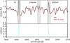 |
Fig. 4 Example of our continuum fit and subtraction performed for the stacked spectrum with SFR = 100.2M⊙ yr-1 and M⋆ = 1010.5M⊙. The top panel shows the observed stacked spectrum (black line) and our best-fit stellar continuum model (red line). The light-gray-shaded regions indicate the wavelength range where the Hβ, [OIII]λ4959 and [OIII]λ5007 emission lines are located. The bottom panel shows the residual spectrum (cyan line) and the level of fluctuations in the fit residuals (dashed line). |
3.2. Fitting the stellar continuum
In order to also reliably measure the weak emission lines emitted by the ionized gas, the stellar continuum must be properly removed. To this end, we use the penalized pixel-fitting (pPXF) algorithm, which is a publicly available IDL code, developed by Cappellari & Emsellem (2004) to find the best fit stellar continuum and separate the nebular emission lines in each stacked spectrum. In brief, pPXF is able to parameterize the line-of-sight velocity distribution (LOSVD) through a Gauss-Hermite expansion of the absorption-line profile by fitting the stellar continuum with a linear combination of simple stellar population (SSP) input model spectra. In the pPXF analysis, we adopt a library of template spectra based on the stellar population models from Bruzual & Charlot (2003), hereafter BC03. BC03 models are available at a resolution of 3 Å FWHM in the wavelength range between 3200 and 9500 Å, which is very similar to the one of SDSS spectra (≈1800 − 2000 between 3800 and 9200 Å). Our templates include a simple stellar population with ages 0.01 ≤ t ≤ 14 Gyr and four different metallicities, Z/Z⊙ = 0.2,0.4,1,2.5 by assuming a Chabrier (2003) initial mass function (IMF). We perform the pPXF analysis for each stacked spectrum in the wavelength range: [4800,5050] Å, where the Hβ, [OIII]λ4959,5007 emission lines are located. The results are a best-fit stellar continuum. For each galaxy bin, we subtract the best-fit stellar continuum from the observed stacked spectrum. This “residual” spectrum is used for any analysis of [OIII]λ5007 emission line features. An example of the fitting procedure result is shown in Fig. 4, which shows the very good agreement of the observed and the model continuum over a large wavelength range in the [OIII] emission line region. In order to check the stability of the fitting procedure and to estimate the error of the residual spectrum, we apply a bootstrapping technique by performing the fit on the sample of bootstrapped stacked spectra in each SFR-stellar mass bin (see previous paragraph). The stability of the procedure is confirmed by the fact that the error of the residual spectrum is consistent or only slightly larger (at maximum 30%) with respect to the error of the stacked spectra. As an example, the panel a) of Fig. 5 shows the residual spectrum in the [OIII]λ5007 emission line region. The quality of our continuum fit is guaranteed by the low level of fluctuations in the fit residuals (dashed lines in Fig. 5). The error of the residual spectrum is then used to estimate the S/N of the emission line in the residual stacked spectra.
For comparison, we also show the result of the continuum subtraction method applied by Mullaney et al. (2013, Fig. 5, panel b). They use, in particular, the single continuum subtracted spectra provided by the SDSS pipeline. While this method turns out to be reasonable for AGN spectra where the emission line has a very high S/N with respect to the continuum, it is not applicable to galaxy spectra with lower S/N emission lines, as in the case considered here.
3.3. Measuring [OIII]λ5007 emission line profiles
We analyze the oxygen line shape with two different approaches: a) By fitting the line with a single and a double Gaussian to identify a possible second broader component with respect to the systemic one; and b) by adopting a non-parametric analysis. The two methods are complementary. The first one allows us to separately study the various components that determine the observed line, while the second procedure is independent to the particular fitting function and is relatively insensitive to the quality of the data (see Perna et al. 2015; Zakamska & Greene 2014; Liu et al. 2013).
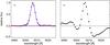 |
Fig. 5 Average [OIII]λ5007 profile of the galaxy subsample with SFR = 100.2M⊙ yr-1 and M⋆ = 1010.5M⊙. In panel a: we show the emission line derived with our method, obtained with the fit and remove of the stellar continuum by pPXF algorithm (see the text for more details). In panel b: we show the emission line for the same SFR and M⋆ galaxies obtained by the continuum-subtracted spectra provided by the SDSS pipeline as shown by Mullaney et al. (2013). Our method is more efficient at modeling and removing the stellar features in the proximity of the [OIII] line. The black symbols are the observed flux. The magenta lines illustrate the two-Gaussian component and the blue curve shows the combined fit. The level of scatter in the residuals of our fit is shown with the horizontal dashed lines. The vertical gray line marks the rest-frame position of the [OIII] line. |
3.3.1. Profile fitting
We fit the [OIII] line profile in the residual spectrum with one and two Gaussian components by using an IDL MPFIT fitting code. In both cases we fit the line center, width and amplitude.
The single Gaussian fit allows us to estimate the global line width, σ[ OIII ], and the S/N of the line. The observed σobs of the line is the convolution of the real width of the emitted line and the instrumental resolution. To remove the instrumental effects, we correct the σobs with ![Mathematical equation: \hbox{$\sigma_{\rm [OIII]}=\sqrt{\sigma_{\rm obs}^{2} - \sigma_{\rm inst}^2}$}](/articles/aa/full_html/2017/10/aa29519-16/aa29519-16-eq93.png) , where
, where  is the instrumental dispersion. For SDSS data, the σinst change as a function of wavelength, and it varies with the location of the object on the plate and the temperature on the night of the observations. Therefore, in order to use the correct σinst for all our stacked spectra, we use the instrumental resolution measured for each single spectrum from the ARC lamps provided by the MPA-JHUgroup (σARC). The final σinst applied in each stacked spectrum isthe median value of the singles σARC. The mean σinst in the [OIII] wavelength range for our sample is ~60 km s-1.
The double Gaussian fit allows us to estimate the significance of a second component and its line profile. We take the double Gaussian profile as the best fit for the [OIII] line profile when it leads to a reduction of the reduced χ2 value by more than 30%. This is to avoid a misidentification of a second component when the double Gaussian fit provides two Gaussian components with consistent width and center and different amplitude. Indeed, in this case the sum of the two Gaussian would lead anyhow to a single Gaussian component. We check that a reduction of the χ2 value by at least 30% is a good threshold to distinguish the need of a double Gaussian fit.
We check the reliability of our multi Gaussian fit by using an additional statistical criterion. To avoid overfitting and allow for the correct number of Gaussian used in each [OIII] line fit, we employed the Bayesian Information Criterion (BIC, Liddle 2007): BIC = χ2 + p ∗ ln(n), where χ2 is the chi squared of the fit, p is the number of free parameters (3 and 6 for one and two Gaussian components, respectively) and n is the number of flux points used in the fit. We measured the BIC value by using the one single Gaussian fit and the double Gaussian fit. The model with the smallest value of the BIC was chosen as the preferred model for the data. We find that the BIC method is perfectly in agreement with the previous method. In the following section, we discriminate between a single or double Gaussian fit on the basis of the BIC.
When the double Gaussian fit is retained as the best fit, we use it to estimate a) the S/N of the second component to check its significance; b) to compare the flux percentage of the second component with respect to the systemic contribution; c) to estimate the velocity shift of the centroid with respect to the systemic redshift; and d) to estimate the line width of the second and systemic component.
The errors on all measured quantities are obtained with a bootstrapping technique. The fit is repeated on the bootstrapping sample (see previous paragraph) to obtain the distribution of all measured quantities, and hence the dispersion as an estimate of the error.
3.3.2. Non-parametric analysis
To have a model-independent measurement of emission line profiles, we also apply a non-parametric approach. This approach is commonly used in AGN outflow studies (Liu et al. 2013; Rupke & Veilleux 2013; Zakamska & Greene 2014; Harrison et al. 2014; Brusa et al. 2015; Perna et al. 2015). Briefly, we construct the cumulative flux of the line as a function of velocity: 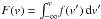 , in the observed spectrum without using any particular fitting function. Then, we describe the velocity width, asymmetry and the wings prominence of the [OIII] line by using the following non-parametric quantities:
- 1.
Velocity width. The velocity width, W80, is the velocity range that encloses 80% of the total flux. It is defined by W80 = v90 − v10, where v90 and v10 are the velocities at which 90% and 10% of the line flux accumulates, respectively. For a purely Gaussian velocity profile the W80 is proportional to the standard deviation (σ) and full width at half maximum (FWHM), as shown in the following equation, W80 = 2.563 × σ = 1.088 × FWHM. Values of W80 are given in km s-1.
- 2.
Asymmetry. The dimensionless parameter R = ((v95 − v50) − (v50 − v05)) / (v95 − v05) gives a measure of the asymmetry of the velocity profile relative to the median velocity. In a perfectly symmetric profile R is R = 0
- 3.
Line wings. The prominence of the line wings in the profile is the non-parametric analog of the kurtosis, with r9050 = W90 /W50, where W90 and W50 are the width comprising 90% and 50% of the flux, W90 = v95 − v05 and W50 = v75 − v25. In a Gaussian profile r9050 is equal to 2.4389 and the r9050 increases in profiles with more extended wings.
The error on each of the quantities is estimated, as in the previous case, via bootstrapping analysis. Each quantity is measured in the bootstrapping sample related to each residual spectrum in order to estimate the dispersion of the distribution as a measure of the error. This is done, in particular, to check if each quantity deviates more than 3σ from the value corresponding to a Gaussian distribution with the same width of the observed line. For this purpose, we use the measure of the global line width estimated with the single Gaussian line profile, as explained in the previous paragraph.
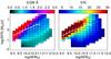 |
Fig. 6 EQW (left panel) and total line-signal-to-noise ratio, (right panel) in the SFR-M⋆ diagram for the total sample. The white line shows the mode and dispersion of the MS. The galaxy bins with total emission line S/N< 8 are plotted in gray. |
4. Results
In this section we first show our results for the total sample (621990 galaxies), then we focus on the results obtained for the six BPT classes: SF, SF−AGN, AGN−SF, LINERs, TYPE2 AGNs (289079 galaxies) and unClass (332911 galaxies). We also show the comparison with the TYPE1 AGN sample of Mullaney et al. 2013; 10 548 galaxies). See Table 1 for percentage values and number of stacked spectra in each sample.
4.1. [OIII] line in the global sample
We analyze the line flux and shape of the total sample, stacked in 148 median spectra (see Sect. 3.1), as a function of position in the SFR-M⋆ diagram. Figure 6 shows the distribution of the [OIII]λ5007 equivalent width (EQW, left panel) and corresponding (S/N, right panel), of the total emission line in the SFR-M⋆ plane. As expected, the MS region is populated by the higher EQW values and higher S/N, while towards the passive region, the line is intrinsically weak, with EQW ≤ 1 Å and low S/N, S/N ≤ 8. In order to ensure a robust and accurate measurement of the total emission line shape, we impose a S/N limit on the [OIII] line of 8. The stacked spectra with [OIII] line detected with S/N> 8 are 94, which correspond to 366 133 galaxies. The median spectra with a low S/N level (54, obtained from 255 857 single galaxies) are preferentially unClass objects, mainly located in the quiescent region, as can be seen from the distribution of different BPT classes in Fig. 3. In the remaining figures here, all bins with total emission line S/N< 8 are plotted in gray and are not considered in the analysis.
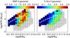 |
Fig. 7 Signal-to-noise ratio and flux enclosed in the second broader Gaussian component (left and right panel) in the SFR-M⋆ diagram for the total sample. The white line shows the mode and dispersion of the MS. The galaxy bins with total emission line S/N< 8 are plotted in gray. |
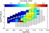 |
Fig. 8 Prominence of the line wings r9050 in the SFR-M⋆ diagram for the total sample. The white line shows the mode and dispersion of the MS. The bins below M⋆ = 1010.5M⊙ have r9050 values consistent with 2.44 within 3σ. The galaxy bins with total emission line S/N< 8 are plotted in gray. |
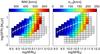 |
Fig. 9 Non-parametric w80 and σ[ OIII ] (left and right panels, respectively) in the SFR-M⋆ diagram for the total sample. The white line shows the mode and dispersion of the MS. |
We use the results of the best Gaussian fit, single or double, to check the significance of the second Gaussian component. When a single Gaussian turns out to be the best fit, we set the S/N of the second component to zero. When the best fit is provided by a double Gaussian, we estimate the S/N of the second component as the ratio between the flux encapsulated in this component and the noise in the region of the line profile. This is done in each bin of the SFR-stellar mass plane. The left panel of Fig. 7 shows the S/N of the second Gaussian component, while the right panel shows the percentage of flux encapsulated in it. Despite the very high S/N of the global [OIII] line (Fig. 6 right panel), the second broad Gaussian component is only marginally detected with a S/N ~ 2.5 − 3 at masses above ~1010M⊙ and in a large range of SFR (Fig. 7 left panel). Al lower masses, the [OIII] line is perfectly consistent with a single Gaussian and no additional component is needed to fit the line profile. The flux encapsulated in the second broad component, though, is less than 10% most of the MS region, with the exception of the highest mass bins, where it reaches a value of 20%; it reaches a similar percentage (20−25%) in the valley between the MS and the quiescent region also.
This is also confirmed by the non-parametric analysis. The values of the line wings parameter, r9050, as a function of the position in the SFR-M⋆ plane, is shown in Fig. 8. The r9050 parameter is consistent with the value of a Gaussian function (r9050 ~ 2.44) along and around the MS relation, up to stellar masses of 1010.5M⊙. The kurtosis is exceeding, with poor significance (~2σ), the Gaussian value up to values of 2.9−3 in the mass range 1010.5 − 11M⊙, where the percentage of flux encapsulated in the broader component is of 20−25%. For comparison, the kurtosis of a Lorentzian profile, with strong wings, is 6.31. In all bins, the [OIII] line appears to be symmetrical, with typical R values always consistent with 0 within 3σ of significance.
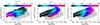 |
Fig. 10 Left panel: σ[ OIII ]/σ⋆ in the SFR-M⋆ plane. At high stellar mass, the gas kinematics follows the velocity dispersion of the stellar component. Central panel: B/T median values in the SFR-M⋆ diagram. The bulge-disk decomposition is taken from the Simard et al. (2011) catalog. We use the values calculated with the r filter. Right panel: σ⋆ distribution in the SFR-M⋆ plane. At low stellar masses the σ⋆ is below to the instrumental resolution. In all panels, the white line shows the mode and dispersion of the MS. |
Figure 9 shows the distribution of the line width in the SFR-M⋆ plane, estimated either with the dispersion σ[ OIII ] and the analogous non-parametric W80 (right and left side, respectively). We observe a progressive increase in the line width with the galaxy stellar mass M⋆, irrespective of SFR. This is expected since the [OIII] emission traces the galaxy potential well. We compare the value of σ[ OIII ] in any bin of the plane with the mean galaxy velocity dispersion, estimated from the absorption features due to the stellar component provided by the MPA-JHU public catalog. The left panel of Fig. 10 shows that at high stellar masses, the ratio between σ[ OIII ] and the galaxy velocity dispersion is consistent with 1. Only at lower masses (<1010.5M⊙) does the ratio increase to higher values. However in this region, none of the previous indicators (flux enclosed in the second broader component, asymmetry R or the kurtosis r9050) show signature of a non Gaussian line profile. Thus, we ascribe such an increase to two factors: a) the galaxies in this region tend to be pure disks, as shown by the mean B/T of ~0.1 as derived from Simard et al. (2011, central panel of Fig. 10), thus the gas could show a different kinematics than the stellar component; b) in this region of the diagram, the MPA-JHU public catalog provides values of the stellar velocity dispersion lower than the SDSS resolution of 70 km s-1, which we assume to be a lower limit (see right panel of Fig. 10).
Thus, we conclude that there is only marginal evidence for a broad component in the [OIII]λ5007 emission line profile and only in a specific locus of the SFR-stellar mass plane. When detected, such a component is centered at the systemic redshift and there is no evidence of a blueshift, as indication of wind, as for the more symmetrical profiles of TYPE 2 AGNs shown in Mullaney et al. (2013). Most of the MS region is well represented by galaxies with [OIII] profile well fitted by a single Gaussian component with no asymmetry and with low kurtosis values. Only at high masses (1010.5 − 1011M⊙) do we observe a marginally higher kurtosis and therefore the presence of line wings. However, for these galaxies, we do not find an excess of the line [OIII] width with respect to the galaxy velocity dispersion provided by the stellar component. Indeed, only a small percentage of the [OIII] flux is encapsulated in the wings. This indicates that likely a low percentage of the gas in these galaxies is moving away in a very low velocity wind.
4.2. Trends with AGN and SF activity
The absence of significant outflow signature in the global population does not exclude the possibility that strong winds might be observed in specific classes of objects. In order to investigate this possibility, in this section we analyze the [OIII] line profile in the BPT subclasses, and so as a function of different ionization sources. As described in Sect. 2 we split our sample into: SF, SF−AGN, AGN−SF, LINERs, TYPE 2, and unClass galaxies. We perform a first analysis on the stacked spectra of each subclass and then we study the stacked spectra as a function of the position in the SFR-M⋆ plane for each subclass separately.
Figure 11 shows our multicomponent emission line fit to the stacked [OIII] line profile of each subclass. It is immediately apparent, that the significance of a second broad and slightly blueshifted component is remarkably increasing with the increase of the AGN contribution. While the star forming galaxy population shows a symmetric Gaussian [OIII] line profile, the increase of the nuclear activity in the SF-AGN and AGN-SF leads to the raise of significant line wings. LINERs, TYPE 2, and TYPE 1 AGN, in particular, also show a more prominent and slightly blueshifted broader component (characterized by a velocity dispersion of 470.1 ± 110.0, 363.1 ± 14.0 and 363.1 ± 14.0 km s-1, respectively) with respect to the systemic velocity (ΔV< 70 km s-1) and corresponding negative values in the asymmetry parameter (R). The flux enclosed in the second Gaussian component goes from 0% in the SF galaxies to 48% in the TYPE 1 AGN, consistently with the result obtained for the TYPE 1 in Mullaney et al. (2013), as shown in Fig. 12.
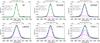 |
Fig. 11 Emission-line profile fits to composite spectra in different classes of photoionization processes: SF, SF−AGN, AGN−SF, LINERs, TYPE 2 and TYPE 1. The black symbols are the observed flux. The flux errors, in each point, are shown in red. The green line shows the single-Gaussian fit. The magenta line illustrates the two-Gaussian component and the blue curve shows the combined fit. The level of scatter in the residuals of our fit is shown with the horizontal dashed red lines. The significance of a second broad and blue-shifted component (magenta curves) is remarkably increasing with the increase of the AGN contribution. In each panel we show the derived values of flux enclosed in the second broader Gaussian component, asymmetry R, prominence of the line wings r9050 and w80. |
The study of the [OIII] line profile of the individual BPT classes as a function of the location in the SFR-stellar mass plane shows the following aspects:
-
SF galaxies, dominating the MS region up to masses of1010M⊙, are characterized by a purely Gaussian [OIII] line profile with no evidence of a second broader component. This is confirmed by the fitting procedure and by the non-parametric method that indicates values of asymmetry and line wings consistent with the Gaussian values within 1.5σ.
-
SF galaxies with a small contribution from the central AGN (SF-AGN) show evidence of a second broader component only at the 2σ level. Such galaxies, as shown in Fig. 3, are mainly located in the MS region at stellar masses >1010M⊙.
-
galaxies with a dominating AGN contribution (AGN-SF) show evidence of a second broader component at more than 3σ only on and above the MS.
-
LINERs and TYPE2 galaxies show a high S/N (>3) second broader component independently of their location on the SFR-stellar mass plane. We refer to Fig. 3 for their distribution in the plane.
-
the results are confirmed by the non-parametric method. The analysis of the asymmetry R shows that for the SF object, the line tends to be symmetrical (R ~ 0) while in the LINERs and TYPE 2, we observe R ~ − 0.1, consistent with the results of Zakamska & Greene (2014) for a sample of SDSS obscured quasars.
An example of the AGN effect on the [OIII] line profile is shown in one mass bin above (left panel), on (central panel) and below (right panel) the MS in Fig. 13.
The location of the AGN-SF, LINERs, and TYPE2 AGNs perfectly matches the location of the plane where we observe in the global population a line wings value slightly larger than the Gaussian value. This is also confirmed by the BPT analysis applied to the stacked spectra, as a function of the location in the SFR-stellar mass plane. As shown in Fig. 14, SF-AGN are preferentially located at high SFR and stellar masses, while AGN-SF and LINERs dominate the valley between the MS and the quiescent region. Indeed, after removing such galaxies from the global sample, the value of the line wings parameter becomes consistent with the Gaussian value all over the plane. This indicates that the deviation from the pure Gaussian behavior observed in Fig. 8 is due to galaxies dominated by the AGN contribution. In turn, this suggests that, if the second broader component is interpreted as an indication of galactic wind, such wind is likely driven by the AGN, while SF does not seem capable of driving any wind at any mass or SFR value.
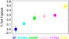 |
Fig. 12 Mean values of the flux percentage enclosed in the second Gaussian component for all the BPT classes: SF,SF-AGN, AGN-SF, LINERs, TYPE 2 and TYPE 1. The flux increases with the increase of the AGN contribution. The error bars show the dispersion around the mean values. |
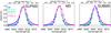 |
Fig. 13 Variation of the observed [OIII] emission line profile as a function of the SF and AGN contribution for galaxies located in different SFR bins. In the left, middle, and right panels we show the galaxy bins located above (SUPMS), inside (MS) and below (SUBMS) the MS, respectively, with ΔSFR = 0.4, 0.0 and − 0.4 dex. The galaxy bins shown have M⋆ = 1010.5M⊙. The [OIII] emission line appears at any M⋆ and SFR. |
In order to better compare the [OIII] line width with respect to the galaxy velocity dispersion in the different subclasses, we show in Fig. 15 the [OIII] line width measured by the standard deviation σ[ OIII ] as a function of stellar velocity dispersion σ⋆ for all the ionization classes: SF, SF−AGN, AGN−SF, LINERs, and TYPE 2. Given that the median instrumental resolution of SDSS spectra is ~70 km s-1 we restrict the analysis to the bins with σ⋆ above this limit. For clarity, we collect our σ[ OIII ] values in bins of σ⋆, with Δσ⋆ = 20 km s-1. The different ionization sources are indicated with different colors as labeled in the figure. At fixed σ⋆, we find that the velocity dispersions measured for the ionized gas increases with the increase of the AGN activity from the “pure” SF to the TYPE 2 galaxies.
As mentioned in Sect. 2.3, the unClass subsample includes a large amount of galaxies (53.5% of the total sample) that are impossible to classify individually using the BPT diagram. In order to take into account this large fraction of galaxies, we decided to perform the BPT analysis in the median stacked spectra. Following the approach of Concas et al. (in prep.) we used a combination of the publicly available codes pPXF (Cappellari & Emsellem 2004) and GANDALF (Sarzi et al. 2006) to fit and remove the stellar continuum and to derive emission line fluxes of the four emission lines used in the BPT diagram (i.e., Hβ, [OIII]λ5007, [NII], Hα). As expected, the majority of the stacked spectra show very weak emission lines. These galaxies are mainly located in the so-called quiescent region as shown in Fig. 3. At higher SFR values, all the unClass stacked spectra show all the four emission lines (Hβ, [OIII]λ5007, [NII] and Hα) with S/N> 4 to classify them in the BPT diagram. We verified that these galaxies follow the same trend shown by the rest of the sample. The prominence of the second broader component increases in parallel to an increase of the nuclear activity contribution, as we can see by the increase of velocity dispersion of the ionized gas with respect to the increase of AGN activity at any stellar velocity dispersion (see triangles in Fig. 15).
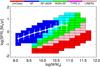 |
Fig. 14 BPT classification for the total sample in the SFR–M⋆ plane. |
5. Discussion and conclusions
In this work we investigate the presence of galactic winds in a large spectroscopic sample of ~600 000 local galaxies drawn from the spectroscopic SDSS DR7 database. In particular, we use the deviation of the forbidden [OIII]λ5007 emission line profile from a Gaussian as a proxy for the galactic winds. We use the spectral stacking technique to increase the S/N of the spectra and to determine how the average [OIII]λ5007 profile changes as a function of the key galaxy physical parameters, such as SFR and M⋆. We also explore how the line profiles relate to the particular photoionization mechanisms: SF or AGN activity. We analyze the oxygen emission line profile by performing a line fit and a non-parametric analysis. Our main results can be summarized as follows:
-
In the global galaxy population, we find no evidence of a second Gaussian broader component in most of the SFR-stellar mass plane. A marginal detection, at the ~2σ level, is obtained only at stellar masses >1010.5M⊙ in a large range of SFR. This is confirmed by the observation of a line width parameter slightly larger (again at the ~2σ level) than the value predicted for a pure Gaussian line profile in the same region of the plane. The line profile appears to be always symmetric, even when a second broader component might contribute. The flux percentage enclosed in the broader component, when detected, is approximately 10% in most of the plane and reaches values of 20−25% at very high masses and SFR and in the valley between the MS and the quiescent region.
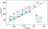
Fig. 15 σ[ OIII ] plotted against σ⋆ MPA-JHU mean values for the five ionization classes (SF, SF−AGN, AGN−SF, LINERs and TYPE 2). We show the median and dispersion values of σ[ OIII ] and σ⋆ in bins of σ⋆, with Δσ⋆ = 20 km s-1. Filled symbols are the objects in the main SF, SF−AGN, AGN−SF, LINERs, and TYPE 2 subsamples. Open triangles are the unClass objects. The solid black line denotes σ[ OIII ] = σ⋆.
-
The comparison of the line width of the [OIII] with the velocity dispersion obtained from the absorption stellar features reveals a good agreement in most of the plane, indicating that the [OIII] traces the underlying galaxy potential well as the stellar component. Only in few very low SFR and stellar mass bins do we observed a disagreement, that we ascribe to spectral resolution issues and differences in the stellar and gas kinematics in purely disk galaxies.
-
The analysis of the [OIII] line profile as a function of the BPT classification reveals that for the “pure” SF galaxies, the ionized interstellar gas traced by the [OIII]λ5007 line never appears to be outflowing. The line profile is perfectly fitted by a single Gaussian without need for a second component. This holds in all the regions of the SFR-stellar mass plane dominated by SF galaxies, such as the MS.
-
The significance of a second broader Gaussian component increases with a clear trend with the increase of the AGN contribution to the galaxy spectrum, with a maximum for the AGN TYPE1 of Mullaney et al. (2013). The flux enclosed in the second component rises steadily from 0% in pure SF galaxies to ~48% in the TYPE1 AGNs.
-
The analysis of the [OIII] line profile of each BPT class in the SFR-stellar mass diagram shows that galaxies with an increasing AGN contribution occupy preferentially the region of the diagram where the global population shows a marginal deviation from the Gaussian line profile: at high mass and SFR and in the valley between the MS and the quiescent region. If AGN hosts are removed from the global sample, such deviations disappear in any locus of the SFR-stellar mass digram. The preferential location of AGN hosts, distinguished in different BPT classes, is also analyzed by performing the BPT analysis on the stacked spectra. We clearly observe a preferential location of galaxies in the diagram as a function of their nuclear activity. In particular, SF-AGN galaxies occupy the region at high stellar mass and SFR, while AGN-SF and LINERs are located preferentially in the valley between the MS and the quiescent region.
-
The comparison of the velocity dispersion obtained from the [OIII] line width with the velocity dispersion derived from the absorption features imprinted by the stellar component shows that the ionized gas traces the galaxy potential well as the stellar component for the pure SF galaxies. The ratio between the two velocity dispersions increases with the increase of the AGN contribution at any bin of stellar velocity dispersion. This, once again, confirms the role of the AGN contribution in leading to a larger [OIII] line width, and so to the presence of winds, independently of the galaxy mass or SFR.
Our results clearly indicate that, when using the low-density ionized gas emission lines as wind indicators, the SF activity itself, in the local Universe, is not capable of driving galactic winds at any value of the instantaneous SF rate or stellar mass. We point out that this outcome is not directly in disagreement with previous findings of outflow signatures in SF galaxies with much higher levels of SF activity, as ULIRGS or high redshift MS star forming galaxies (e.g., Heckman et al. 1990; Pettini et al. 2000; Shapley et al. 2003; Rupke et al. 2002, 2005a,b; Martin 2005, 2006; Hill & Zakamska 2014). Indeed, such systems exhibit SFR level at least one order of magnitude higher than the level of activity in the local average star forming galaxies. Thus, we cannot exclude that star formation might be capable of driving outflow when feedback is sufficiently energetic to induce motion. Our results indicate, however, that, at the level of activity observed in the local Universe, SF feedback is not capable of inducing significant gas bulk motions. A direct comparison with a similar sample of galaxies at higher redshift, and so with a higher level of SF activity, must be carried out to determine the SF threshold, above which SF might eventually lead to systematic galactic winds.
This result, however, contrasts the findings of Cicone et al. (2016), who detect signatures of ionized outflows in local SDSS star forming galaxies at high SFR. They also find an increase of the line width with increasing SFR at fixed mass, and interpret this as evidence of SF driven outflow. We ascribe such discrepancy to the differences in the sample selection. Cicone et al. (2016) analyze a sample of ~160 000 local star forming galaxies classified in the BPT diagram according to Kauffmann et al. (2003a). As shown in Stasinska et al. (2006), these selection criteria may introduce a significant bias in the SF galaxy sample, due to the inclusion of a large percentage of systems with an AGN contribution. This effect may be particularly strong at high SFRs where the number of composite SF−AGN is high. In order to investigate this issue, we perform our analysis on the “HII” sample of star forming galaxies as defined in Cicone et al. (2016). As Cicone et al. (2016), we do not find any significant broad second Gaussian component for the galaxies located at low SFR and M⋆, while we note a weak increase of this second component (~10% of the total line flux, ~2σ level) at SFR ≥ 1 M⊙/yr and stellar masses M⋆ ≥ 1010M⊙ (Fig. 16). However, by classifying the Cicone et al. (2016) “HII” sample with the Stasinska et al. (2006) BPT classification, as done for our sample, we see (Fig. 17) that
-
pure SF galaxies consistently show a pure Gaussian profile withconstant width at fixed stellar mass;
-
SF−AGN galaxies show a more prominent second Gaussian component, although of low significance (<2σ), a larger width with respect to pure SF galaxies of the same mass and SFR, and an increase of the width with increasing SFR at fixed stellar mass.
We, thus, conclude that the effect observed by Cicone et al. (2016) is likely due to the contamination by systems with an AGN contribution. The larger width of the [OIII] profile at high SFR in such galaxies could be due to availability of a large quantity of cold gas, which favors at the same time the SF activity and accretion onto the central black hole, eventually leading to stronger BH feedback. We also point out that the transition between pure SF galaxies and AGN-contaminated galaxies takes place in the region of the diagram that starts to be dominated by bulgier sources (see central panel of Fig. 10). This is a further indication that the central activity might be a bias in the analysis performed by Cicone et al. (2016).
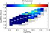 |
Fig. 16 S/N of the second broader Gaussian component for the “HII” galaxy sample in the SFR-M⋆. The white line shows the mode and dispersion of the MS. At high SFR and M⋆ the S/N shows a slight increase. The galaxy bins with total emission line S/N< 8 are plotted in gray. |
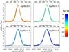 |
Fig. 17 Comparison in four different stellar mass bins of the observed [OIII] line profile of pure SF (gray curves) and SF-AGN galaxies (color curves) in the HII sample, classified according to the BPT classification of Stasinska et al. (2006). The line profile of the pure SF galaxies does not change as a function of the SF level. For this reason, in each mass bin, we only show a single curve concerning one level of SFR. The line profile of the SF-AGN galaxies tends to increase in width at increasing SFR as indicated by the several curves color-coded as a function of the SFR. |
Our results confirm the role of AGN feedback in leading to galactic wind, at least of ionized gas, in the local Universe. This result is in agreement with many recent findings in a large redshift window. At low redshift, we find very good agreement with the results of Mullaney et al. (2013), that observe a prominent blueshifted and broader Gaussian component in addition to the systemic one for TYPE 1 and TYPE 2 AGNs. Our analysis extends this result to a lower level of nuclear activity also. While the use of the fiber SDSS spectra does not allow us to have any spatial information on the origin and the location of the wind, by using the optical integral field unit (IFU) observations of sixteen TYPE 2 AGN selected from the Mullaney et al. (2013) parent sample. Harrison et al. (2014) demonstrate that this particular [OIII] emission line feature is due to the kiloparsec scale outflows, extended over ≥6−16 kpc.
At higher redshift, Harrison et al. (2016) find a high prevalence of extreme ionized gas velocities in high-luminosity X-ray AGN. Moreover, Brusa et al. (2015) and Cresci et al. (2015) show that in X-ray-bright AGN, the nuclear activity can lead to very powerful winds, of the order of ~1000 km s-1, also in the molecular gas.
We point out that, on average, we do not observe such large velocity shift or line width. The observed average velocity shift with respect to the systemic redshift is below the SDSS instrumental resolution ΔV< 70 km s-1, and the line width of the second Gaussian component is only of the order of 350−400 km s-1 also in the BPT classes, which include an AGN contribution. Thus, rather than galactic wind, the overall population of AGN hosts in the local Universe undergo a phase of light “breeze”. This difference might arise for two reasons: a) Bright X-ray AGNs are rare objects in the local Universe, thus, the average velocity shift and line width is dominated by sources with a lower level of nuclear activity and feedback; b) we are observing a final phase of the wind, which was more powerful in the past due to the higher nuclear activity of the central AGN.
Since the AGN hosts are located in the high-mass region of the SFR-stellar mass diagram at stellar masses M⋆ ≥ 1010.5M⊙, and are thus likely to be in dark matter halos larger than 1012 − 12.5M⊙, such velocities are at least one order of magnitude lower than the escape velocity from the galaxy. Therefore, the gas entrained in the wind is very unlikely to be capable of escaping the galaxy potential well.
Thus, we conclude that, through the identification of strong bulk motion as traced by the warm ionized gas, at least in the local Universe, the AGN activity is likely the only mechanism capable of driving galactic winds. However, given the velocity of such winds, the gas in this scenario is not capable of escaping from the galaxy and thus affecting the galaxy gas content and SF activity.
Acknowledgments
The authors are grateful to the anonymous referee, whose suggestions improved this manuscript. M.B. thanks the DFG cluster of excellence “Origin and Structure of the Universe” (www.universe-cluster.de) for partial support during the completion of this work, and acknowledges support from the FP7 Career Integration Grant “aEASy” (CIG 321913).
References
- Abazajian, K. N., Adelman-McCarthy, J. K., Agüeros, M. A., et al. 2009, ApJS, 182, 543 [NASA ADS] [CrossRef] [Google Scholar]
- Arribas, S., Colina, L., Bellocchi, E., Maiolino, R., & Villar-Martín, M. 2014, A&A, 568, A14 [NASA ADS] [CrossRef] [EDP Sciences] [Google Scholar]
- Baldry, I., Glazebrook, K., & Driver, S. 2008, MNRAS, 388, 945 [NASA ADS] [Google Scholar]
- Baldwin, J. A., Phillips, M. M., & Terlevich, R. 1981, PASP, 93, 5 [NASA ADS] [CrossRef] [EDP Sciences] [Google Scholar]
- Behroozi, P. S., Conroy, C., & Wechsler, R. H. 2010, ApJ, 717, 379 [NASA ADS] [CrossRef] [Google Scholar]
- Behroozi, P. S., Wechsler, R. H., & Conroy, C. 2013, ApJ, 770, 57 [NASA ADS] [CrossRef] [Google Scholar]
- Bellocchi, E., Arribas, S., Colina, L., & Miralles-Caballero, D. 2013, A&A, 557, A59 [NASA ADS] [CrossRef] [EDP Sciences] [Google Scholar]
- Bower, R. G., Benson, A. J., Malbon, R., et al. 2006, MNRAS, 370, 645 [NASA ADS] [CrossRef] [Google Scholar]
- Brinchmann, J., Charlot, S., White, S., et al. 2004, MNRAS, 351, 1151 [NASA ADS] [CrossRef] [Google Scholar]
- Brusa, M., Bongiorno, A., Cresci, G., Perna, M., et al. 2015, MNRAS, 446, 2394 [NASA ADS] [CrossRef] [Google Scholar]
- Bruzual, G., & Charlot, S. 2003, MNRAS, 344, 1000 [NASA ADS] [CrossRef] [Google Scholar]
- Cano-Díaz, M., Maiolino, R., Marconi, A., et al. 2012, A&A, 537, L8 [NASA ADS] [CrossRef] [EDP Sciences] [Google Scholar]
- Cappellari, M., & Emsellem, E. 2004, PASP, 116, 138 [NASA ADS] [CrossRef] [Google Scholar]
- Carniani, S., Marconi, A., Maiolino, R., et al. 2015, A&A, 580, A102 [NASA ADS] [CrossRef] [EDP Sciences] [Google Scholar]
- Cazzoli, S., Arribas, S., Colina, L., et al. 2014, A&A, 569, A14 [NASA ADS] [CrossRef] [EDP Sciences] [Google Scholar]
- Chabrier, G. 2003, PASP, 115, 763 [NASA ADS] [CrossRef] [Google Scholar]
- Chen, Y.-M., Tremonti, C., Heckman, T., et al. 2010, AJ, 140, 445 [NASA ADS] [CrossRef] [Google Scholar]
- Chevalier, R. A. 1977, ARA&A, 15, 175 [NASA ADS] [CrossRef] [Google Scholar]
- Cicone, C., Maiolino, R., Sturm, E., et al. 2014, A&A, 562, A21 [NASA ADS] [CrossRef] [EDP Sciences] [Google Scholar]
- Cicone, C., Maiolino, R., & Marconi, A. 2016, A&A, 588, A41 [NASA ADS] [CrossRef] [EDP Sciences] [Google Scholar]
- Conroy, C., & Wechsler, R. H. 2009, ApJ, 696, 620 [NASA ADS] [CrossRef] [Google Scholar]
- Cresci, G., Mainieri, V., Brusa, M., et al. 2015, ApJ, 799, 82 [Google Scholar]
- Croton, D. J., Springel, V.White, S. D. M., et al. 2006, MNRAS, 365, 11 [NASA ADS] [CrossRef] [Google Scholar]
- De Lucia, G., Springel, V., White, S., Croton, D., & Kauffmann, G. 2006, MNRAS, 366, 499 [NASA ADS] [CrossRef] [Google Scholar]
- Di Matteo, T., Springel, V., & Hernquist, L. 2005, Nature, 433, 604 [NASA ADS] [CrossRef] [PubMed] [Google Scholar]
- Erb, D. 2015, Nature, 523, 169 [NASA ADS] [CrossRef] [Google Scholar]
- Fabian, A. 2012, ARA&A, 50, 455 [NASA ADS] [CrossRef] [Google Scholar]
- Feruglio, C., Maiolino, R., Piconcelli, E., et al. 2010, A&A, 518, L155 [NASA ADS] [CrossRef] [EDP Sciences] [Google Scholar]
- Förster Schreiber, N. M., Genzel, R., Newman, S. F., et al. 2014, ApJ, 787, 38 [NASA ADS] [CrossRef] [Google Scholar]
- Genzel, R., Förster Schreiber, N. M., Rosario, D., et al. 2014, ApJ, 796, 7 [Google Scholar]
- Greene, J., & Ho, L. 2005, ApJ, 627, 721 [NASA ADS] [CrossRef] [Google Scholar]
- Greene, J. E., Zakamska, N., & Smith, P. 2012, ApJ, 746, 86 [NASA ADS] [CrossRef] [Google Scholar]
- Guo, Q., White, S., Li, C., & Boylan-Kolchin, M. 2010, MNRAS, 404, 1111 [NASA ADS] [Google Scholar]
- Guo, Q., White, S., Boylan-Kolchin, M., et al. 2011, MNRAS, 413, 101 [NASA ADS] [CrossRef] [Google Scholar]
- Harrison, C. M., Alexander, D. M., Swinbank, A. M., et al. 2012, MNRAS, 426, 1073 [NASA ADS] [CrossRef] [Google Scholar]
- Harrison, C., Alexander, D. M., Mullaney, J. R., & Swinbank, A. M. 2014, MNRAS, 441, 3306 [Google Scholar]
- Harrison, C. M., Alexander, D. M., Mullaney, J. R., et al. 2016, MNRAS, 456, 1195 [NASA ADS] [CrossRef] [Google Scholar]
- Heckman, T., Armus, L., & Miley, G. 1990, ApJS, 74, 833 [NASA ADS] [CrossRef] [Google Scholar]
- Henriques, B. M. B., White, S. D. M., Thomas, P. A., et al. 2017, MNRAS, 469, 2626 [Google Scholar]
- Hill, M. J., & Zakamska, N. 2014, MNRAS, 439, 2701 [NASA ADS] [CrossRef] [Google Scholar]
- Hopkins, P., Hernquist, L., Cox, T. J., Robertson, B., & Springel, V. et al. 2006, ApJS, 163, 50 [NASA ADS] [CrossRef] [Google Scholar]
- Hopkins, P. F., Kereš, D., Oñorbe, J., et al. 2014, MNRAS, 445, 581 [NASA ADS] [CrossRef] [Google Scholar]
- Kauffmann, G., Heckman, T. M., Tremonti, C., et al. 2003a, MNRAS, 346, 1055 [Google Scholar]
- Kauffmann, G., Heckman, T. M., White, S. D. M., et al. 2003b, MNRAS, 341, 54 [Google Scholar]
- Kewley, L., Dopita, M., Sutherland, R., Heisler, C., & Trevena, J. 2001, ApJ, 556, 121 [Google Scholar]
- Kewley, L., Groves, B., Kauffmann, G., & Heckman, T. 2006, MNRAS, 372, 961 [NASA ADS] [CrossRef] [Google Scholar]
- Lehnert, M. D., & Heckman, T. M. 1996, ApJ, 472, 546 [NASA ADS] [CrossRef] [Google Scholar]
- Liddle, A. R. 2007, MNRAS, 377, L74 [NASA ADS] [Google Scholar]
- Lilly, S., Le Fevre, O., Hammer, F., & Crampton, D. 1996, ApJ, 460, L1 [NASA ADS] [CrossRef] [Google Scholar]
- Liu, G., Zakamska, N., Greene, J., Nesvadba, N., & Liu, X. 2013, MNRAS, 436, 2576 [NASA ADS] [CrossRef] [Google Scholar]
- Madau, P., & Dickinson, M. 2014, ARA&A, 52, 415 [NASA ADS] [CrossRef] [Google Scholar]
- Madau, P., Ferguson, H. C., Dickinson, M., et al. 1996, MNRAS, 283, 1388 [NASA ADS] [CrossRef] [Google Scholar]
- Madau, P., Pozzetti, L., & Dickinson, M. 1998, ApJ, 498, 106 [NASA ADS] [CrossRef] [Google Scholar]
- Maiolino, R., Gallerani, S., Neri, R., et al. 2012, MNRAS, 425, L66 [NASA ADS] [CrossRef] [Google Scholar]
- Martin, C. 2005, ApJ, 621, 227 [Google Scholar]
- Martin, C. 2006, ApJ, 647, 222 [NASA ADS] [CrossRef] [Google Scholar]
- Martin, C., Shapley, A. E., Coil, A. L., et al. 2012, ApJ, 760, 127 [NASA ADS] [CrossRef] [Google Scholar]
- Morselli, L., Popesso, P., Erfanianfar, G., & Concas, A. 2017, A&A, 597, A97 [NASA ADS] [CrossRef] [EDP Sciences] [Google Scholar]
- Moster, B. P., Somerville, R., Maulbetsch, C., et al. 2010, ApJ, 710, 903 [NASA ADS] [CrossRef] [Google Scholar]
- Moster, B. P., Naab, T., & White, S. 2013, MNRAS, 428, 3121 [NASA ADS] [CrossRef] [Google Scholar]
- Mullaney, J. R., Alexander, D. M., Fine, S., et al. 2013, MNRAS, 433, 622 [NASA ADS] [CrossRef] [Google Scholar]
- Murray, N., Quataert, E., & Thompson, T. A. 2005, ApJ, 618, 569 [NASA ADS] [CrossRef] [Google Scholar]
- Newman, S. F., Genzel, R., Förster-Schreiber, N. M., et al. 2012, ApJ, 761, 43 [NASA ADS] [CrossRef] [Google Scholar]
- Perna, M., Brusa, M., Salvato, M., et al. 2015, A&A, 583, A72 [NASA ADS] [CrossRef] [EDP Sciences] [Google Scholar]
- Pettini, M., Steidel, C., Adelberger, K., Dickinson, M., & Giovalisco, M. 2000, ApJ, 528, 96 [NASA ADS] [CrossRef] [Google Scholar]
- Renzini, A., & Peng, Y.-J. 2015, ApJ, 801, L29 [NASA ADS] [CrossRef] [Google Scholar]
- Rodríguez Zaurín, J., Tadhunter, C. N., Rose, M., & Holt, J. 2013, MNRAS, 432, 138 [NASA ADS] [CrossRef] [Google Scholar]
- Rubin, K. H. R., Prochaska, J. X., Koo, D. C., et al. 2014, ApJ, 794, 156 [NASA ADS] [CrossRef] [Google Scholar]
- Rupke, D., & Veilleux, S. 2011, ApJ, 729, L27 [NASA ADS] [CrossRef] [Google Scholar]
- Rupke, D., & Veilleux, S. 2013, ApJ, 768, 75 [NASA ADS] [CrossRef] [Google Scholar]
- Rupke, D., Veilleux, S., & Sanders, D. 2002, ApJ, 570, 588 [NASA ADS] [CrossRef] [Google Scholar]
- Rupke, D., Veilleux, S., & Sanders, D. 2005a, ApJ, 160, 87 [Google Scholar]
- Rupke, D., Veilleux, S., & Sanders, D. 2005b, ApJ, 160, 115 [Google Scholar]
- Salim, J., Rich, R. M., Charlot, S., et al. 2007, ApJS, 173, 267 [NASA ADS] [CrossRef] [Google Scholar]
- Sarzi, M., Falcón-Barroso, J., Davies, R. L., et al. 2006, MNRAS, 366, 1151 [NASA ADS] [CrossRef] [Google Scholar]
- Schlegel, D., Finkbeiner, D., & Davis, M. 1998, ApJ, 500, 525 [NASA ADS] [CrossRef] [Google Scholar]
- Shapiro, K. L., Genzel, R., Quataert, E., et al. 2009, ApJ, 701, 955 [NASA ADS] [CrossRef] [Google Scholar]
- Shapley, A., Steidel, C., Pettini, M., & Adelberger, K. 2003, ApJ, 588, 65 [NASA ADS] [CrossRef] [Google Scholar]
- Simard, L., Mendel, J. T., Patton, D. R., Ellison, S. L., & McConnachie, A. W. 2011, ApJS, 196, 11 [NASA ADS] [CrossRef] [Google Scholar]
- Soto, K. T., Martin, C. L., Prescott, M. K. M., & Armus, L. 2012, ApJ, 757, 86 [NASA ADS] [CrossRef] [Google Scholar]
- Stasinska, G., Cid Fernandes, R., Mateus, A., Sodré, L., & Asari, N. V. 2006, MNRAS, 371, 972 [NASA ADS] [CrossRef] [Google Scholar]
- Steidel, C. C., Erb, D. K., Shapley, A. E., et al. 2010, ApJ, 717, 289 [NASA ADS] [CrossRef] [Google Scholar]
- Strauss, M. A., Weinberg, D. H., Lupton, R. H., et al. 2002, AJ, 124, 1810 [NASA ADS] [CrossRef] [Google Scholar]
- Tremonti, C. A., Moustakas, J., & Diamond-Stanic, A. 2007, ApJ, 663, L77 [NASA ADS] [CrossRef] [Google Scholar]
- Veilleux, S., & Osterbrock, D. E. 1987, ApJS, 63, 295 [NASA ADS] [CrossRef] [Google Scholar]
- Veilleux, S., Kim, D.-C., Sanders, D. B., Mazzarella, J. M., & Soifer, B. T. 1995, ApJS, 98, 171 [NASA ADS] [CrossRef] [Google Scholar]
- Veilleux, S., Cecil, G., & Bland-Hawthorn, J. 2005, ARA&A, 43, 769 [Google Scholar]
- Villar-Martín, M., Humphrey, A., Delgado, R. G., Colina, L., & Arribas, S. 2011, MNRAS, 418, 2032 [NASA ADS] [CrossRef] [Google Scholar]
- Westmoquette, M. S., Clements, D. L., Bendo, G. J., & Khan, S. A. 2012, MNRAS, 424, 416 [NASA ADS] [CrossRef] [Google Scholar]
- Yang, X., Mo, H. J., van den Bosch, F. C., Zhang, Y., & Han, J. 2012, ApJ, 752, 41 [NASA ADS] [CrossRef] [Google Scholar]
- York, D. G., Adelman, J., Anderson, J. E., Jr., et al. 2000, AJ, 120, 1579 [CrossRef] [Google Scholar]
- Zakamska, N., & Greene, J. 2014, MNRAS, 442, 784 [NASA ADS] [CrossRef] [Google Scholar]
All Tables
All Figures
|
Fig. 1 SFR-M⋆ plane for DR7 SDSS galaxies. The black boxes represent the fine grid used for the stacking of the total sample.The white line shows the position of the so-called “main sequence” (MS) of star−forming galaxies. The MS is computed as the mode and the dispersion of the SFR distribution in stellar mass bins following the example of Renzini & Peng (2015). |
| In the text | |
|
Fig. 2 Distribution of the galaxies in our sample in the BPT line-ratio diagram. The solid curve is the theoretical demarcation of Kewley et al. (2001) , that separates star-forming galaxies and composites from AGN. The dashed (Kauffmann et al. 2003a ) and dotted Stasinska et al. (2006) curves indicate the empirical division between composite SF-AGN and AGN-SF and the pure star-forming galaxies, respectively (see text for more details). The horizontal line at log ([OIII]/Hβ) = 0.5 is the demarcation criteria between TYPE 2 (or Seyfert, Sy) and LINERs galaxies showed in Kewley et al. (2006). |
| In the text | |
|
Fig. 3 Location of SF, SF−AGN, AGN−SF, LINERs, TYPE 2 (or Sy) and unClass galaxies in the SFR-M⋆ plane. From outside to inside, the contours encompass 25, 50, and 75 per cent of the data points. The black line shows the mode and dispersion of the MS. |
| In the text | |
|
Fig. 4 Example of our continuum fit and subtraction performed for the stacked spectrum with SFR = 100.2M⊙ yr-1 and M⋆ = 1010.5M⊙. The top panel shows the observed stacked spectrum (black line) and our best-fit stellar continuum model (red line). The light-gray-shaded regions indicate the wavelength range where the Hβ, [OIII]λ4959 and [OIII]λ5007 emission lines are located. The bottom panel shows the residual spectrum (cyan line) and the level of fluctuations in the fit residuals (dashed line). |
| In the text | |
|
Fig. 5 Average [OIII]λ5007 profile of the galaxy subsample with SFR = 100.2M⊙ yr-1 and M⋆ = 1010.5M⊙. In panel a: we show the emission line derived with our method, obtained with the fit and remove of the stellar continuum by pPXF algorithm (see the text for more details). In panel b: we show the emission line for the same SFR and M⋆ galaxies obtained by the continuum-subtracted spectra provided by the SDSS pipeline as shown by Mullaney et al. (2013). Our method is more efficient at modeling and removing the stellar features in the proximity of the [OIII] line. The black symbols are the observed flux. The magenta lines illustrate the two-Gaussian component and the blue curve shows the combined fit. The level of scatter in the residuals of our fit is shown with the horizontal dashed lines. The vertical gray line marks the rest-frame position of the [OIII] line. |
| In the text | |
|
Fig. 6 EQW (left panel) and total line-signal-to-noise ratio, (right panel) in the SFR-M⋆ diagram for the total sample. The white line shows the mode and dispersion of the MS. The galaxy bins with total emission line S/N< 8 are plotted in gray. |
| In the text | |
|
Fig. 7 Signal-to-noise ratio and flux enclosed in the second broader Gaussian component (left and right panel) in the SFR-M⋆ diagram for the total sample. The white line shows the mode and dispersion of the MS. The galaxy bins with total emission line S/N< 8 are plotted in gray. |
| In the text | |
|
Fig. 8 Prominence of the line wings r9050 in the SFR-M⋆ diagram for the total sample. The white line shows the mode and dispersion of the MS. The bins below M⋆ = 1010.5M⊙ have r9050 values consistent with 2.44 within 3σ. The galaxy bins with total emission line S/N< 8 are plotted in gray. |
| In the text | |
|
Fig. 9 Non-parametric w80 and σ[ OIII ] (left and right panels, respectively) in the SFR-M⋆ diagram for the total sample. The white line shows the mode and dispersion of the MS. |
| In the text | |
|
Fig. 10 Left panel: σ[ OIII ]/σ⋆ in the SFR-M⋆ plane. At high stellar mass, the gas kinematics follows the velocity dispersion of the stellar component. Central panel: B/T median values in the SFR-M⋆ diagram. The bulge-disk decomposition is taken from the Simard et al. (2011) catalog. We use the values calculated with the r filter. Right panel: σ⋆ distribution in the SFR-M⋆ plane. At low stellar masses the σ⋆ is below to the instrumental resolution. In all panels, the white line shows the mode and dispersion of the MS. |
| In the text | |
|
Fig. 11 Emission-line profile fits to composite spectra in different classes of photoionization processes: SF, SF−AGN, AGN−SF, LINERs, TYPE 2 and TYPE 1. The black symbols are the observed flux. The flux errors, in each point, are shown in red. The green line shows the single-Gaussian fit. The magenta line illustrates the two-Gaussian component and the blue curve shows the combined fit. The level of scatter in the residuals of our fit is shown with the horizontal dashed red lines. The significance of a second broad and blue-shifted component (magenta curves) is remarkably increasing with the increase of the AGN contribution. In each panel we show the derived values of flux enclosed in the second broader Gaussian component, asymmetry R, prominence of the line wings r9050 and w80. |
| In the text | |
|
Fig. 12 Mean values of the flux percentage enclosed in the second Gaussian component for all the BPT classes: SF,SF-AGN, AGN-SF, LINERs, TYPE 2 and TYPE 1. The flux increases with the increase of the AGN contribution. The error bars show the dispersion around the mean values. |
| In the text | |
|
Fig. 13 Variation of the observed [OIII] emission line profile as a function of the SF and AGN contribution for galaxies located in different SFR bins. In the left, middle, and right panels we show the galaxy bins located above (SUPMS), inside (MS) and below (SUBMS) the MS, respectively, with ΔSFR = 0.4, 0.0 and − 0.4 dex. The galaxy bins shown have M⋆ = 1010.5M⊙. The [OIII] emission line appears at any M⋆ and SFR. |
| In the text | |
|
Fig. 14 BPT classification for the total sample in the SFR–M⋆ plane. |
| In the text | |
|
Fig. 15 σ[ OIII ] plotted against σ⋆ MPA-JHU mean values for the five ionization classes (SF, SF−AGN, AGN−SF, LINERs and TYPE 2). We show the median and dispersion values of σ[ OIII ] and σ⋆ in bins of σ⋆, with Δσ⋆ = 20 km s-1. Filled symbols are the objects in the main SF, SF−AGN, AGN−SF, LINERs, and TYPE 2 subsamples. Open triangles are the unClass objects. The solid black line denotes σ[ OIII ] = σ⋆. |
| In the text | |
|
Fig. 16 S/N of the second broader Gaussian component for the “HII” galaxy sample in the SFR-M⋆. The white line shows the mode and dispersion of the MS. At high SFR and M⋆ the S/N shows a slight increase. The galaxy bins with total emission line S/N< 8 are plotted in gray. |
| In the text | |
|
Fig. 17 Comparison in four different stellar mass bins of the observed [OIII] line profile of pure SF (gray curves) and SF-AGN galaxies (color curves) in the HII sample, classified according to the BPT classification of Stasinska et al. (2006). The line profile of the pure SF galaxies does not change as a function of the SF level. For this reason, in each mass bin, we only show a single curve concerning one level of SFR. The line profile of the SF-AGN galaxies tends to increase in width at increasing SFR as indicated by the several curves color-coded as a function of the SFR. |
| In the text | |
Current usage metrics show cumulative count of Article Views (full-text article views including HTML views, PDF and ePub downloads, according to the available data) and Abstracts Views on Vision4Press platform.
Data correspond to usage on the plateform after 2015. The current usage metrics is available 48-96 hours after online publication and is updated daily on week days.
Initial download of the metrics may take a while.